hep-th/0309195

Spontaneous localization of bulk fields: the six-dimensional case

Hyun Min Lee, Hans Peter Nilles and Max Zucker

Physikalisches Institut der Universität Bonn,

Nussallee 12, 53115 Bonn, Germany.

Abstract

We study $N=2$ supersymmetric gauge theories with $d=6$ bulk and $d=4$ brane fields charged under a U(1) gauge symmetry. Radiatively induced Fayet-Iliopoulos terms lead to an instability of the bulk fields. We compute the profile of the bulk zero modes and observe the phenomenon of spontaneous localization towards the position of the branes. While this mechanism is quite similar to the $d=5$ case, the mass spectrum of the excited Kaluza-Klein modes shows a crucial difference.

1 Introduction

Recently there has been a revived interest in higher dimensional field theories. A particular fascinating picture is the so-called brane world scenario, where different fields might be confined to space-times (branes) of different dimensionality. Such a picture is expected to be ultimately part of a low-energy description of some more fundamental theory as e.g. string or M-theory. In fact, prototypes of this picture can be found in string theory orbifold compactification [1] as well as the Horava-Witten heterotic $E_{8}\times E_{8}$ - M-theory [2]. In the latter case gravitational fields propagate in the full $d=11$ space-time dimensions while gauge (and matter) fields are confined to the $d=10$ boundaries of the $d=11$ interval. Orbifold compactifications of string theory typically contain untwisted and (various) twisted sectors, where fields propagate in various sub-spaces confined to fixed points (or surfaces) in the compactified dimensions.

In the attempt to construct realistic models for particle physics one therefore generically faces the situation where e.g. quarks, leptons or Higgs bosons originate from fields of different dimensionalities [3, 4]. Such a situation is in fact quite interesting from the phenomenological point of view as the “overlap” of the wave function of the fields in extra dimensions determines various coupling constants in the low energy effective field theory. Mass relations between quarks and leptons might therefore originate from such a higher dimensional mechanism.

Unfortunately, a detailed discussion of these issues is quite difficult. While the set-up is usually simple when one discusses the picture at tree level, complications arise in the quantum theory. The tree level results, however, are modified substantially even in supersymmetric theories. In fact, it has been pointed out that instabilities appear in many models with U(1) gauge groups due to the presence of radiatively induced Fayet-Iliopoulos (FI)-terms [5]. This is particularly relevant for phenomenological applications, as the standard model of particle physics contains the U(1) group of hypercharge.

We are thus interested in a set-up where we have simultaneous existence of brane fields of lower and bulk fields of higher dimensionality. Not much is known about the actual profiles of bulk fields in the presence of brane fields. Work up to now has concentrated on the situation of co-dimension one, i.e. $d=5$ bulk fields and $d=4$ brane fields [6]. There it was shown that the wave function of the bulk zero mode was in general instable in the presence of FI-terms and that this instability could lead to a spontaneous localization of bulk fields at one of the lower dimensional branes. In this dimensional transmutation [7], the bulk field became a brane field and all excited Kaluza-Klein excitations became heavy and decoupled.

It is not clear yet, how such a mechanism could be understood in the framework of string theory. The local structure of tadpoles and anomalies has been studied in the framework of heterotic string theory [8, 9, 10], but the explicit profile of wave functions of the bulk field has not been determined yet as the situation is far more complicated than in the co-dimension one case. The latter might also not be relevant in all cases, as e. g. in heterotic string compactification extra dimensions naturally appear in complex pairs. Fields typically live in even dimensions, $d=10$ for the untwisted fields and $d=4$ and/or $d=6$ for the twisted fields. Therefore it would be appropriate to study the case of even co-dimension.

In the present paper we consider the simplest case: $d=4$ brane fields and $d=6$ bulk fields. This discussion should be understood as a building block to eventually go towards the full $d=10$ theory. It illustrates the specific features of the theory with compactified complex dimension in a framework where explicit calculations can be performed (despite the fact of the missing off-shell formulation of $d=6$ supersymmetry for hypermultiplets). Effective potential, ground state wave function and mass spectrum of the bulk fields can be determined. We show that the presence of localized FI-tadpoles leads to a localization phenomenon similar to the $d=5$ (co-dimension one) case. The mass spectrum of the Kaluza-Klein modes, however, reveals a profound difference to the co-dimension one situation. The $d=6$ bulk field retains its six dimensional nature and the dimensional transmutation of the bulk field to a brane field seems to be a particular property of the co-dimension one case. This might have important consequences for the discussion of localized anomalies.

The paper is organized as follows. In section 2 we give the set-up of supersymmetry of the $T^{2}/{\bf Z}_{2}$ orbifold. Section 3 presents the FI-tadpoles in the $d=6$ case. This is followed in section 4 with the derivation of the effective potential, its minimization and the calculation of mass spectrum and zero-mode wave function. Section 5 discusses possible embeddings in existing string models and the question of anomaly cancellation by (variants of) the Green-Schwarz mechanism. In section 6 we give some concluding remarks.

2 Supersymmetry on $T^{2}/{\bf Z}_{2}$

In this section we describe in detail our model: a six-dimensional $N=2$ super Yang-Mills multiplet with gauge group $U(1)$, coupled to several hypermultiplets. This theory is compactified on the orbifold $T^{2}/{\bf Z}_{2}$. In addition, we have chiral multiplets, living on the fixed points of the orbifold. They are charged under the $U(1)$.

2.1 The super Yang-Mills multiplet

The $N=2$ super Yang-Mills multiplet in six dimensions contains as propagating fields the gauge field $A_{M}$ and the gaugino $\Omega$, which is a right handed symplectic Majorana-Weyl fermion, satisfying the chirality condition (our conventions are collected in appendix A)

$$\Gamma^{7}\Omega=\Omega.$$ (1)

The gaugino is an eight-component object and a doublet under $SU(2)_{\cal R}$. Beside these two propagating fields, there is an auxiliary field $\vec{D}$ which is a triplet under the $SU(2)_{\cal R}$. The action for abelian gauge group is

$${\cal L}=-\frac{1}{4}F_{MN}F^{MN}+i\bar{\Omega}\Gamma^{M}\partial_{M}\Omega+\frac{1}{2}\vec{D}^{2}.$$ (2)

The Lagrangian is invariant under (rigid) supersymmetry:

$$\delta A_{M} = i\bar{\varepsilon}\Gamma_{M}\Omega$$ (3)

$$\delta\Omega = \frac{1}{4}\Gamma^{MN}\varepsilon F_{MN}-\frac{i}{2}\vec{\tau}\varepsilon\vec{D}$$ (4)

$$\delta\vec{D} = \bar{\varepsilon}\vec{\tau}\Gamma^{M}\partial_{M}\Omega.$$ (5)

The supersymmetry parameter $\varepsilon$ is also a right handed symplectic Majorana-Weyl fermion, satisfying a similar relation as the gaugino, eq. (1).

The $\Gamma$-matrices are $8\times 8$ matrices. By using the chiral representation given in (108)-(111), the chirality constraints can be solved, i.e. we can work in a four-dimensional Weyl representation. Defining for an arbitrary spinor

$$\psi={\psi_{L}\choose\psi_{R}}$$ (6)

and using the $4\times 4$ matrices

$$\gamma^{A}\equiv(\gamma^{a},\gamma^{5},-\mathord{\!\leavevmode\hbox{ \begin{picture}(0.6,0.7)\put(0.0,0.0){\line(1,0){0.5}} \put(0.15,0.0){\line(0,1){0.7}} \put(0.35,0.0){\line(0,1){0.8}} \put(0.3,0.8){\rule{0.5pt}{0.5pt}}\put(0.26,0.78){\rule{0.5pt}{0.5pt}}\put(0.22,0.76){\rule{0.5pt}{0.5pt}}\put(0.18,0.74){\rule{0.5pt}{0.5pt}}\put(0.14,0.72){\rule{0.5pt}{0.5pt}}\put(0.1,0.7){\rule{0.5pt}{0.5pt}}\put(0.06,0.68){\rule{0.5pt}{0.5pt}}\put(0.02,0.66){\rule{0.5pt}{0.5pt}}\put(-0.02,0.64){\rule{0.5pt}{0.5pt}}\put(-0.06,0.62){\rule{0.5pt}{0.5pt}}\put(-0.1,0.6){\rule{0.5pt}{0.5pt}}\put(-0.14,0.58){\rule{0.5pt}{0.5pt}} \end{picture}}}_{4})\qquad\mbox{and}\qquad\bar{\gamma}^{A}\equiv(\gamma^{a},\gamma^{5},\mathord{\!\leavevmode\hbox{ \begin{picture}(0.6,0.7)\put(0.0,0.0){\line(1,0){0.5}} \put(0.15,0.0){\line(0,1){0.7}} \put(0.35,0.0){\line(0,1){0.8}} \put(0.3,0.8){\rule{0.5pt}{0.5pt}}\put(0.26,0.78){\rule{0.5pt}{0.5pt}}\put(0.22,0.76){\rule{0.5pt}{0.5pt}}\put(0.18,0.74){\rule{0.5pt}{0.5pt}}\put(0.14,0.72){\rule{0.5pt}{0.5pt}}\put(0.1,0.7){\rule{0.5pt}{0.5pt}}\put(0.06,0.68){\rule{0.5pt}{0.5pt}}\put(0.02,0.66){\rule{0.5pt}{0.5pt}}\put(-0.02,0.64){\rule{0.5pt}{0.5pt}}\put(-0.06,0.62){\rule{0.5pt}{0.5pt}}\put(-0.1,0.6){\rule{0.5pt}{0.5pt}}\put(-0.14,0.58){\rule{0.5pt}{0.5pt}} \end{picture}}}_{4}),$$ (7)

the action (2) can be rewritten as

$${\cal L}=-\frac{1}{4}F_{MN}F^{MN}+i\bar{\Omega}_{R}\gamma^{M}\partial_{M}\Omega_{R}+\frac{1}{2}\vec{D}^{2}.$$ (8)

The transformation laws become

$$\delta A_{M} = i\bar{\varepsilon}_{R}\gamma_{M}\Omega_{R}$$ (9)

$$\delta\Omega_{R} = \frac{1}{4}\gamma^{MN}\varepsilon_{R}F_{MN}-\frac{i}{2}\vec{\tau}\varepsilon_{R}\vec{D}$$ (10)

$$\delta\vec{D} = \bar{\varepsilon}_{R}\vec{\tau}\gamma^{M}\partial_{M}\Omega_{R}.$$ (11)

The symplectic Majorana condition for the right-handed Dirac gaugino becomes

$${\bar{\Omega}}_{Ri}=\varepsilon_{ij}(\Omega^{j}_{R})^{T}{\cal C},$$ (12)

where ${\cal C}$ is the five-dimensional charge conjugation as given in the appendix. Then, we can solve this condition by writing the gaugino in terms of one Dirac spinor $\chi$ as

$$\Omega_{R}^{i}=\left(\begin{array}[]{l}\,\,\,\,\chi\\ {\cal C}{\bar{\chi}}^{T}\end{array}\right).$$ (15)

Similarly, we can also solve the chirality condition for $\varepsilon_{R}$. By dimensionally reducing the super Yang-Mills multiplet to five dimensions and comparing with the known results [11, 12], one can check the consistency of the present theory.

2.2 The hypermultiplet

The other multiplet needed is the hypermultiplet. For this multiplet there is no off-shell formulation possible, since this would require the fields to be charged under central charge transformations. However, in contrast to five dimensions [11], in six-dimensional $N=2$ supersymmetry there is no central charge, which is due to the fact that $d=6$ is the highest dimension where $N=2$ supersymmetry can exist. Fortunately, the non-existence of an off-shell formulation poses no problem for our purposes.

The $r$ hypermultiplets contain $4r$ real scalars $A_{i}^{\alpha}$ and the hyperino $\zeta^{\alpha}$, where the gauge index has to run over an even number of values, $\alpha,\beta=1,\ldots,2r$. The generators of the representation are anti-hermitian $t^{\alpha}{}_{\beta}=-t_{\beta}{}^{\alpha}$, where $t_{\beta}{}^{\alpha}=(t^{\beta}{}_{\alpha})^{*}$. The bosons transform in the $\bf 2$ of $SU(2)_{\cal R}$, whereas the fermions are singlets. The scalars $A_{i}^{\alpha}$ satisfy a reality condition

$$A^{i}_{\alpha}\equiv A_{i}^{\alpha*}=\varepsilon^{ij}\rho_{\alpha\beta}A_{j}^{\beta}$$ (16)

where $\rho$ can be choosen to be $\rho=\mathord{\!\leavevmode\hbox{ \begin{picture}(0.6,0.7)\put(0.0,0.0){\line(1,0){0.5}} \put(0.15,0.0){\line(0,1){0.7}} \put(0.35,0.0){\line(0,1){0.8}} \put(0.3,0.8){\rule{0.5pt}{0.5pt}}\put(0.26,0.78){\rule{0.5pt}{0.5pt}}\put(0.22,0.76){\rule{0.5pt}{0.5pt}}\put(0.18,0.74){\rule{0.5pt}{0.5pt}}\put(0.14,0.72){\rule{0.5pt}{0.5pt}}\put(0.1,0.7){\rule{0.5pt}{0.5pt}}\put(0.06,0.68){\rule{0.5pt}{0.5pt}}\put(0.02,0.66){\rule{0.5pt}{0.5pt}}\put(-0.02,0.64){\rule{0.5pt}{0.5pt}}\put(-0.06,0.62){\rule{0.5pt}{0.5pt}}\put(-0.1,0.6){\rule{0.5pt}{0.5pt}}\put(-0.14,0.58){\rule{0.5pt}{0.5pt}} \end{picture}}}\otimes\varepsilon$, as shown in [13]. Consistency requires a reality constraint on the generators of the gauge group,

$$t^{\alpha}{}_{\beta}=-\rho^{\alpha\gamma}t_{\gamma}{}^{\delta}\rho_{\delta\beta}.\$$ (17)

The chirality of the hyperino is opposite to the one of the gaugino, i.e.

$$\Gamma^{7}\zeta^{\alpha}=-\zeta^{\alpha}.$$ (18)

The supersymmetry transformation laws together with the reality constraint (16) induce a reality constraint for the hyperino,

$$\bar{\zeta}_{\alpha}=-\rho_{\alpha\beta}{\zeta^{\beta}}^{T}C,$$ (19)

where the Dirac conjugate is defined in the standard way (cf. eq. (112)).

The supersymmetry transformation laws we find are

$$\delta A_{i}^{\alpha} = i\bar{\varepsilon}_{i}\zeta^{\alpha}$$ (20)

$$\delta\zeta^{\alpha} = -\Gamma^{A}\varepsilon^{i}{\cal D}_{A}A_{i}^{\alpha},$$ (21)

with covariant derivative

$${\cal D}_{M}A_{i}^{\alpha}=\partial_{M}A_{i}^{\alpha}-g(A_{M})^{\alpha}{}_{\beta}A_{i}^{\beta}.$$ (22)

The supersymmetry algebra closes only up to equations of motion.

The hypermultiplet Lagrangian is

$${\cal L}=\frac{1}{2}{\cal D}_{M}A_{i}^{\alpha}{\cal D}^{M}A^{i}_{\alpha}+\frac{i}{2}\bar{\zeta}_{\alpha}\Gamma^{M}{\cal D}_{M}\zeta^{\alpha}-2ig\bar{\zeta}_{\alpha}\Omega^{i\alpha}{}_{\beta}A^{\beta}_{i}+\frac{ig}{2}(\vec{\tau})^{i}{}_{j}A_{i}^{\alpha}A^{j}_{\beta}\vec{D}^{\beta}{}_{\alpha}.$$ (23)

We can again use the chiral basis (108)-(111) which we used already for the super Yang-Mills multiplet. The Lagrangian then becomes

$${\cal L}=\frac{1}{2}{\cal D}_{M}A_{i}^{\alpha}{\cal D}^{M}A^{i}_{\alpha}+\frac{i}{2}\bar{\zeta}_{L\alpha}\bar{\gamma}^{M}{\cal D}_{M}\zeta^{\alpha}_{L}-2ig\bar{\zeta}_{L\alpha}\Omega_{R}^{i\alpha}{}_{\beta}A^{\beta}_{i}+\frac{ig}{2}(\vec{\tau})^{i}{}_{j}A_{i}^{\alpha}A^{j}_{\beta}\vec{D}^{\beta}{}_{\alpha}$$ (24)

and the transformation laws read

$$\delta A_{i}^{\alpha} = i\bar{\varepsilon}_{Ri}\zeta^{\alpha}_{L}$$ (25)

$$\delta\zeta^{\alpha}_{L} = -\gamma^{A}\varepsilon^{i}_{R}{\cal D}_{A}A_{i}^{\alpha}.$$ (26)

We can rewrite the Lagrangian in a better suited way. To this end, we introduce a two component field [14]

$$A_{i}^{\hat{\alpha}(i)}={A_{i}^{2\hat{\alpha}-1}\choose A_{i}^{2\hat{\alpha}}},$$ (27)

where the hatted index runs over $\hat{\alpha}=1,\ldots,r$ and the index in brackets denotes the two entries in the object on the r.h.s. The reality constraint (16) now becomes diagonal,

$$A^{i}_{\hat{\alpha}(i)}=\delta_{\hat{\alpha}\hat{\beta}}\varepsilon_{(i)(j)}\varepsilon^{ij}A_{j}^{\hat{\beta}(j)}.$$ (28)

This equation can easily be solved by introducing complex fields $\phi_{\pm}$

$$A_{i}^{\hat{\alpha}(i)}\equiv\left(\begin{array}[]{cc}A_{1}^{\hat{\alpha}(1)}&A_{2}^{\hat{\alpha}(1)}\\ A_{1}^{\hat{\alpha}(2)}&A_{2}^{\hat{\alpha}(2)}\\ \end{array}\right)=\left(\begin{array}[]{cc}\phi_{-}^{*\hat{\alpha}}&\phi_{+}^{\hat{\alpha}}\\ -\phi_{+}^{*\hat{\alpha}}&\phi_{-}^{\hat{\alpha}}\\ \end{array}\right),$$ (29)

which makes the underlying quaternionic structure more explicit (cf. [13, 14, 15]). The meaning of the index $\pm$ will become clear when we orbifold the hypermultiplet.

Likewise, the reality constraint (19) for the hyperino with a two component field $\zeta^{{\hat{\alpha}}(i)}_{L}$ becomes

$$\bar{\zeta}_{L{\hat{\alpha}}(i)}=\delta_{{\hat{\alpha}}{\hat{\beta}}}\varepsilon_{(i)(j)}(\zeta^{{\hat{\beta}}(j)}_{L})^{T}{\cal C}.$$ (30)

Then, this equation is solved by introducing one Dirac spinor $\psi$ as

$$\zeta^{{\hat{\alpha}}(i)}_{L}=\left(\begin{array}[]{l}\,\,\,\,\,\,\,\,\psi\\ {\cal C}{\bar{\psi}}^{T}\end{array}\right).$$ (33)

Using the $\phi_{\pm}$ and $\psi$ fields, the relevant hypermultiplet Lagrangian from eq. (24) becomes (suppressing $\hat{\alpha}$-indices)

$${\cal L}=\sum_{\pm}\left({\cal D}_{M}\phi_{\pm}^{\dagger}{\cal D}^{M}\phi_{\pm}\mp g\phi_{\pm}^{\dagger}q\phi_{\pm}D_{3}\right)+i{\bar{\psi}}\bar{\gamma}^{M}{\cal D}_{M}\psi+\ldots.$$ (34)

Here we have chosen the gauge group to be $U(1)$ and the generators to be $t=iQ=-iq\otimes\tau^{3}$, with diagonal charge matrices $Q$ and $q$. The covariant derivatives are

$${\cal D}_{M}\phi_{\pm}=\partial_{M}\phi_{\pm}\pm igq\phi_{\pm}A_{M}.$$ (35)

2.3 Orbifolding

We now consider our theory given by the sum of the actions (8) and (24) on the orbifold $T^{2}/{\bf Z}_{2}$. The coordinates which form the torus are $x^{5}$ and $x^{6}$ with radii $R_{5}$ and $R_{6}$, respectively. The ${\bf Z}_{2}$ acts like

$${\bf Z}_{2}:\qquad(x^{5},x^{6})\to(-x^{5},-x^{6}).$$ (36)

So the $T^{2}/{\bf Z}_{2}$ orbifold has four fixed points,

$$(x^{5},x^{6})=\qquad(0,0),\qquad(\pi R_{5},0),\qquad(0,\pi R_{6}),\qquad\mbox{and}\qquad(\pi R_{5},\pi R_{6}).$$ (37)

A boson is either even (${\cal P}=+1$) or odd (${\cal P}=-1$) under the ${\bf Z}_{2}$. The parities $\cal P$ of the bosons belonging to the super Yang Mills multiplet are collected in the table.

Field	$A_{m}$	$A_{5}$	$A_{6}$	$D_{1}$	$D_{2}$	$D_{3}$
Parity $\cal P$	$+1$	$-1$	$-1$	$-1$	$-1$	$+1$

Table 1: Parities of the super Yang-Mills multiplet.

The gaugino transforms like

$$\Omega(x^{m},x^{5},x^{6})\to-i\tau^{3}\Gamma_{5}\Gamma_{6}\Omega(x^{m},-x^{5},-x^{6})$$ (38)

which becomes in the chiral representation we used repeatedly

$$\Omega(x^{m},x^{5},x^{6})_{R}\to i\tau^{3}\gamma^{5}\Omega(x^{m},-x^{5},-x^{6})_{R}.$$ (39)

At the fixed points, the even fields form a four-dimensional $N=1$ super Yang-Mills multiplet with field content

$$(A_{m},\Omega_{R},-D_{3}+F_{56}),$$ (40)

i.e. the four-dimensional auxiliary field is not $D_{3}$ as one might have naively expected but $-D_{3}+F_{56}$. We can compare this to the five-dimensional result (see, e.g. [16, 6, 7]). There the four-dimensional auxiliary field was given by $-D_{3}+\partial_{5}\Phi$, where $\Phi$ is to be identified with $A_{6}$. So $-D_{3}+F_{56}$ is the gauge covariant generalization of $-D_{3}+\partial_{5}\Phi$.

The orbifolding of the hypermultiplet is most easily written down using the $\phi_{\pm}$-fields. One finds

$${\bf Z}_{2}:\qquad\phi_{\pm}^{\hat{\alpha}}\to\pm\phi_{\pm}^{\hat{\alpha}}$$ (41)

and for the hyperino

$$\zeta^{\hat{\alpha}(i)}_{L}\to i(\tau^{3})^{(i)}{}_{(j)}\gamma^{5}\zeta^{\hat{\alpha}(j)}_{L}.$$ (42)

2.4 Chiral multiplets at the fixed points

As stated above, the super Yang-Mills multiplet forms a four-dimensional super Yang-Mills multiplet at the fixed points. In the spirit of Mirabelli and Peskin [16], we can couple chiral multiplets which live at the fixed points to the super Yang-Mills multiplet. Our formalism is chosen to agree at the fixed points with the one in [6, 7], so our Lagrangian is the same as given there. For completeness, we should give it here:

$${\cal L} = \sum_{I=1}^{4}\delta(x^{5}-x^{5}_{I})\delta(x^{6}-x^{6}_{I})\Big{[}{\cal D}_{m}\phi_{I}^{\dagger}{\cal D}^{m}\phi_{I}$$ (43)

$$+ i\bar{\psi}_{I\ell}\gamma^{m}{\cal D}_{m}\psi_{I\ell}+f^{\dagger}_{I}f_{I}+g\phi^{\dagger}_{I}q_{I}\phi_{I}(-D_{3}+F_{56})+\cdots\Big{]}.$$

$(x^{5}_{I},x^{6}_{I})$ label the fixed points as given in (37). $q_{I}$ are the charge matrices at the fixed points. More details on the boundary Lagrangian may be found in [6, 7].

3 Tadpoles

We want to calculate the tadpole diagrams which generate Fayet-Iliopoulos terms at the branes. The procedure is exactly as in [6, 7] and the result can be obtained accordingly. We shall therefore not present the details of the calculation here.

The tadpole diagrams contain the hyperons $\phi_{\pm}$ and the hyperinos $\psi$ as well as the charged brane scalars $\phi_{I}$.

As discussed above, the $D$ field belonging to the four-dimensional super Yang-Mills multiplet is given by $D=-D_{3}+F_{56}$. So the form of our Fayet-Iliopoulos term is

$${\cal L}_{FI}=\xi(-D_{3}+F_{56}).$$ (44)

There are two types of contributions to $\xi$, one from the bulk, the other one from the branes,

$$\xi=\xi_{bulk}+\xi_{branes}$$ (45)

with

$$\xi_{bulk}=\frac{1}{4}g~{}{\rm tr}(q)\left(\frac{\Lambda^{2}}{16\pi^{2}}+\frac{1}{4}\frac{\ln\Lambda^{2}}{16\pi^{2}}(\partial_{5}^{2}+\partial_{6}^{2})\right)\sum_{I}\delta(x^{5}-x^{5}_{I})\delta(x^{6}-x^{6}_{I})$$ (46)

and

$$\xi_{brane}=g\frac{\Lambda^{2}}{16\pi^{2}}\sum_{I}{\rm tr}(q_{I})\delta(x^{5}-x^{5}_{I})\delta(x^{6}-x^{6}_{I}).$$ (47)

This result for $\xi$ is, of course, similar to the one obtained in the five-dimensional $S^{1}/{\bf Z}_{2}$ model [6, 7]: The main difference is an additional factor of $1/2$ in $\xi_{bulk}$ due to the double number of fixed points in our model. The only other difference $\partial^{2}_{5}\to\partial_{5}^{2}+\partial_{6}^{2}$ should be clear. The brane contributions are unchanged.

We reshuffle the contributions and write the Fayet-Iliopoulos term as the sum of quadratically divergent and logarithmically divergent pieces:

$$\xi=\sum_{I}\left(\xi_{I}+\xi^{\prime\prime}(\partial_{5}^{2}+\partial_{6}^{2})\right)\delta(x^{5}-x^{5}_{I})\delta(x^{6}-x^{6}_{I})$$ (48)

with

$$\xi_{I} = \frac{1}{16\pi^{2}}g\Lambda^{2}\left(\frac{1}{4}{\rm tr}(q)+{\rm tr}(q_{I})\right),$$ (49)

$$\xi^{\prime\prime} = \frac{1}{16}\frac{1}{16\pi^{2}}g\ln\Lambda^{2}{\rm tr}(q).$$ (50)

The distribution of quadratic FI tadpoles $\xi_{I}$’s on the orbifold is shown in Fig. 1.

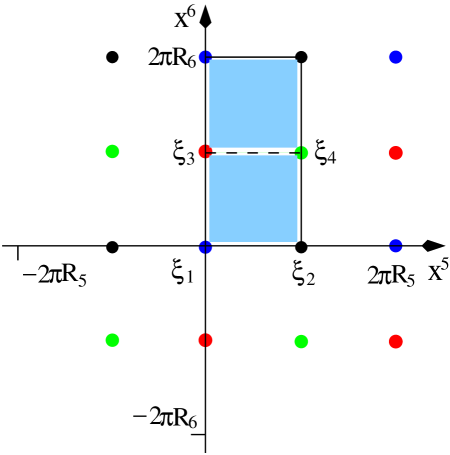
Figure 1: The distribution of localized Fayet-Iliopoulos tadpoles on a $T^{2}/{\bf Z}_{2}$ orbifold. The shaded region is the fundamental region of the orbifold.

4 The effective potential

It is now easy to write down the effective four-dimensional potential; we simply collect all pieces of the action which give rise to the potential in the four-dimensional theory:

$$V = \int dx^{5}dx^{6}\Big{[}2g^{2}|\phi^{T}_{+}q\phi_{-}|^{2}+\sum_{\pm}({\cal D}_{5}\phi_{\pm}+i{\cal D}_{6}\phi_{\pm})^{\dagger}({\cal D}_{5}\phi_{\pm}+i{\cal D}_{6}\phi_{\pm})$$ (51)

$$+ \frac{1}{2}\Big{(}F_{56}-g(\phi_{+}^{\dagger}q\phi_{+}-\phi_{-}^{\dagger}q\phi_{-})-\xi-g\sum_{I}\delta(x^{5}-x^{5}_{I})\delta(x^{6}-x^{6}_{I})\phi^{\dagger}_{I}q_{I}\phi_{I}\Big{)}^{2}$$

$$- \frac{1}{2}\Big{(}D_{3}-g(\phi_{+}^{\dagger}q\phi_{+}-\phi_{-}^{\dagger}q\phi_{-})-\xi-g\sum_{I}\delta(x^{5}-x^{5}_{I})\delta(x^{6}-x^{6}_{I})\phi^{\dagger}_{I}q_{I}\phi_{I}\Big{)}^{2}$$

$$- \frac{1}{2}(D_{1}+g\phi^{T}_{+}q\phi_{-}+g\phi^{\dagger}_{-}q\phi_{+}^{*})^{2}-\frac{1}{2}(D_{2}+ig\phi^{T}_{+}q\phi_{-}-ig\phi^{\dagger}_{-}q\phi_{+}^{*})^{2}\Big{]}$$

A consistency check is to show that unbroken supersymmetry is equivalent to vanishing potential. After elimination of the auxiliary fields, the potential is positive semi-definite.

The conditions for unbroken supersymmetry are

$$D_{3}=F_{56}=g(\phi_{+}^{\dagger}q\phi_{+}-\phi_{-}^{\dagger}q\phi_{-})+\xi+g\sum_{I}\delta(x^{5}-x^{5}_{I})\delta(x^{6}-x^{6}_{I})\phi^{\dagger}_{I}q_{I}\phi_{I}$$ (52)

together with

$$\phi_{+}^{T}q\phi_{-}=0$$ (53)

and

$${\cal D}_{5}\phi_{\pm}+i{\cal D}_{6}\phi_{\pm}=0.$$ (54)

4.1 Supersymmetric background solutions

Now suppose that our ground state does not break the $U(1)$, i.e. $\langle\phi_{\pm}\rangle=\langle\phi_{I}\rangle=0$. Then, the supersymmetry condition (52) becomes

$$\langle F_{56}\rangle=\xi.$$ (55)

When we integrate this equation over the extra dimensions, Stokes theorem with no boundary gives

$$0=\int^{\pi R_{5}}_{0}dx^{5}\int^{\pi R_{6}}_{0}dx^{6}\langle F_{56}\rangle=\sum_{I}\xi_{I},$$ (56)

which means

$${\rm tr}(q)+{\rm tr}(q_{1})+{\rm tr}(q_{2})+{\rm tr}(q_{3})+{\rm tr}(q_{4})=0.$$ (57)

This consistency condition ensures the absence of overall mixed gauge-gravitational anomalies. If (57) is violated, we would expect the U(1) to be broken at a high scale either spontaneously or through a variant of a Green-Schwarz mechanism. We shall come back to this question in section 5.

Now let us introduce complex coordinates

$$z=\frac{1}{R_{5}}x^{5}+\frac{1}{R_{6}}\tau x^{6},$$ (58)

with the torus modulus $\tau=iR_{6}/R_{5}$. By this definition, the periodicities on the torus are

$$z\simeq z+2\pi\simeq z+2\pi\tau.$$ (59)

A key obervation is the fact that we can solve eq. (55) with the following ansatz:

$$\langle A_{5}\rangle=-\partial_{6}W\qquad\mbox{and}\qquad\langle A_{6}\rangle=\partial_{5}W,$$ (60)

where $W$ must be even under ${\bf Z}_{2}$. Please note that by taking this ansatz we have fixed the gauge implicitly. Defining

$$W^{\prime}=2\left(W-\frac{2}{R^{2}_{5}}\sum_{I}\xi^{\prime\prime}\delta^{2}(z-z_{I})\right),$$ (61)

eq. (55) becomes

$$\partial\bar{\partial}W^{\prime}=\sum_{I}\xi_{I}\delta^{2}(z-z_{I}),$$ (62)

which is some sort of Poisson equation.

The solution to eq. (62) can be deduced from string theory: $W^{\prime}$ is the propagator of a bosonic string for a toroidal world sheet, see e.g. [17]. The modular invariant and periodic solution to (62) on the torus is then

$$W^{\prime}=\frac{1}{2\pi}\sum_{I}\xi_{I}\left[\ln\left|\vartheta_{1}\left(\frac{z-z_{I}}{2\pi}\big{|}\tau\right)\right|^{2}-\frac{1}{2\pi\tau_{2}}[{\rm Im}(z-z_{I})]^{2}\right]$$ (63)

where $\tau_{2}={\rm Im}\tau=R_{6}/R_{5}$. Note that in order for $W^{\prime}$ in the above to be a solution to (62), eq. (57) has to hold. We can also check that $W^{\prime}$ is invariant under ${\bf Z}_{2}$ as required from eqs. (60) and (61).

4.2 Localization of the bulk zero mode

Now we are in the position to consider the solution for the zero mode in the presence of the background solution. The equation for the bulk zero mode is the same as eq. (54). Defining the complex potential $A=A_{5}-iA_{6}$ in the complex coordinates from eq. (58) and using the background solution with $A=-(2i/R_{5})\partial W$ from eq. (60), the equation for the zero mode becomes

$$({\bar{\partial}}-gq{\bar{\partial}}W)\phi_{+}=0.$$ (64)

Thus, from eqs. (61) and (63), we obtain the exact solution for the zero mode as

$$\phi_{+} = f_{+}(z)e^{gqW}$$ (65)

$$= f_{+}(z)\prod_{I}\left|\vartheta_{1}\left(\frac{z-z_{I}}{2\pi}\big{|}\tau\right)\right|^{\frac{1}{2\pi}gq\xi_{I}}\times$$

$$\times \exp\left[-\frac{1}{8\pi^{2}\tau_{2}}gq\xi_{I}[{\rm Im}(z-z_{I})]^{2}+\frac{gq\xi^{\prime\prime}}{R^{2}_{5}}\delta^{2}(z-z_{I})\right],$$

where $f_{+}(z)$ is a holomorphic function of $z$. Since $f_{+}(z)$ is an analytic function in the whole complex plane where ${\bar{\partial}}f_{+}=0$, it should be a constant which is determined by the normalization condition

$$1=\int_{0}^{\pi R_{5}}dx^{5}\int_{0}^{\pi R_{6}}dx^{6}|\phi_{+}|^{2}.$$ (66)

Let us now discuss the localization of the zero mode. There are three factors to be discussed from the wave function of the zero mode (65): the $\vartheta_{1}$ term, the $e^{({\rm Im})^{2}}$ term and the $e^{\delta^{2}}$ term. The second one implies a (de)localization behavior of zero mode at $z=z_{I}$ with $q\xi_{I}<0(q\xi_{I}>0)$. From the asymptotic limit of the theta function for $z\rightarrow z^{\prime}$

$$\vartheta_{1}\bigg{(}\frac{z-z^{\prime}}{2\pi}|\tau\bigg{)}\rightarrow(\eta(\tau))^{3}(z-z^{\prime}),$$ (67)

where $\eta(\tau)$ is the Dedekind eta function, we can see that the wave function of the zero mode becomes divergent at the fixed points where $q\xi_{I}<0$. In fact, from eq. (57), at least one of the $\xi_{I}$’s should take a different sign from the others, so it would imply the strong localization of the zero mode at up to three fixed points at the same time. Moreover, the $e^{\delta^{2}}$ term also seems to give a strong (de)localization for $q\xi^{\prime\prime}>0(q\xi^{\prime\prime}<0)$ as in the five-dimensional case [6]. Thus the $\vartheta_{1}$ term with $q\xi_{I}<0$ and the $e^{\delta^{2}}$ term need to be regularized.

By inserting a simple regularization of the delta function in eqs. (61) and (62) with

$$\delta^{2}(z-z_{I})=\left\{\begin{array}[]{l}\frac{R^{2}_{5}}{\pi\rho^{2}},\qquad|z-z_{I}|<\rho/R_{5},\\ 0,\qquad\,\,\,\,|z-z_{I}|>\rho/R_{5},\end{array}\right.$$ (70)

and omitting the normalization, the regularized zero mode function for $|z-z_{I}|\ll 1$ is given for a finite $\rho$ with $\rho\ll R_{5}$ as

$$\phi_{+}\simeq\left\{\begin{array}[]{l}\exp\bigg{[}\frac{gq}{4\pi}\xi_{I}\ln\big{(}\frac{\rho^{2}}{R^{2}_{5}}\big{)}+\frac{gq\xi^{\prime\prime}}{\pi\rho^{2}}\bigg{]},\qquad|z-z_{I}|<\rho/R_{5},\\ \exp\bigg{[}\frac{gq}{4\pi}\xi_{I}\bigg{(}\ln(|z-z_{I}|^{2})-\frac{1}{2\pi\tau_{2}}[{\rm Im}(z-z_{I})]^{2}\bigg{)}\bigg{]},\,\,\rho/R_{5}<|z-z_{I}|\ll 1.\end{array}\right.$$ (73)

To understand the localization of the zero mode explicitely we have to maintain two regularization scales: the momentum cutoff $\Lambda$ and the brane thickness $\rho$; both $\rho$ and $1/\Lambda$ are small compared to $R_{5},R_{6}$. The localization induced by $\xi$ is typically exponential in $\Lambda$ while the one induced by $\xi^{\prime\prime}$ is power like. Thus as long as $\rho$ is not very small compared to $1/\Lambda$ the effect of the logarithmic FI-term will be subleading (naturally one could expect $\rho$ and $1/\Lambda$ to be of the same order of magnitude). In addition, as we shall see in the next section, the logarithmic FI-term does not effect the mass spectrum of the bulk field at all.

4.3 Mass spectrum

Making a Kaluza-Klein reduction to $d=4$, the equation for the massive modes with nonzero gauge field background is given by

$$(-{\cal D}_{5}+i{\cal D}_{6})({\cal D}_{5}+i{\cal D}_{6})\phi_{\pm}=m^{2}\phi_{\pm}.$$ (74)

Then, this equation can be rewritten in terms of the scalar function $W$, given by the gauge field solutions in eq. (60), as

$$(\partial\pm gq\partial W)(\bar{\partial}\mp gq\bar{\partial}W)\phi_{\pm}=-\frac{1}{4}m^{2}R^{2}_{5}\phi_{\pm}.$$ (75)

By substituting in eq. (75)

$$\phi_{\pm}=e^{\pm gqW}\tilde{\phi}_{\pm},$$ (76)

we get a simpler form

$$\partial\bar{\partial}\tilde{\phi}_{\pm}\pm 2gq\partial W\bar{\partial}\tilde{\phi}_{\pm}=-\frac{m^{2}}{4}R_{5}^{2}\tilde{\phi}_{\pm}.$$ (77)

Since there appear derivatives of delta functions in this equation, we need to regularize the delta function. Let us take the regularizing function to be

$$\Delta^{2}(z-z_{I})=\left\{\begin{array}[]{cl}\frac{R^{2}_{5}}{\pi\rho^{2}_{I}}\bigg{(}1-\frac{R^{2}_{5}|z-z_{I}|^{2}}{\rho^{2}_{I}}\bigg{)},&\mbox{for }|z-z_{I}|<\rho_{I}/R_{5},\\ 0,&\mbox{for }|z-z_{I}|>\rho_{I}/R_{5},\end{array}\right.$$ (80)

where $\rho_{I}$ corresponds to the thickness of the $z=z_{I}$ brane. Here one can easily check that $\lim_{\rho_{I}\rightarrow 0}\int d^{2}z^{\prime}\Delta^{2}(z-z^{\prime})h(z^{\prime},{\bar{z}}^{\prime})=h(z,{\bar{z}})$ for an arbitrary complex function $h$. Then, the solution for $W$ given in eq. (61) becomes

$$W=\frac{1}{2}\int d^{2}z^{\prime}\,G(z-z^{\prime})\sum_{I}\xi_{I}\Delta^{2}(z^{\prime}-z_{I})+\frac{2}{R^{2}_{5}}\sum_{I}\xi^{\prime\prime}\Delta^{2}(z-z_{I}),$$ (81)

where $G(z-z^{\prime})$ is the string propagator on the torus satisfying ${\bar{\partial}}\partial G(z-z^{\prime})=\delta^{2}(z-z^{\prime})-1/(8\pi^{2}\tau_{2})$. In order for $W$ to be periodic on the torus, which is necessary even in view of the zero mode in eq. (65), we need the same regularization of branes, i.e. the same $\rho_{I}$’s. In this case, we again have the zero sum $\sum_{I}\xi_{I}=0$. Consequently, we get the holomorphic derivative of $W$ as

$$\partial W=\frac{1}{2}\sum_{I}\xi_{I}\int d^{2}z^{\prime}\,\partial G(z-z^{\prime})\Delta^{2}(z^{\prime}-z_{I})+\frac{2}{R^{2}_{5}}\sum_{I}\xi^{\prime\prime}\partial\Delta^{2}(z-z_{I}).$$ (82)

Now let us consider the region outside the brane where $\partial W$ is holomorphic because ${\bar{\partial}}(\partial W)=0$. Then, for $|z-z_{I}|>\rho_{I}/R_{5}$, eq. (77) becomes solvable with a separation of variables as ${\tilde{\phi}}_{\pm}=\chi_{\pm}(z)\,\varphi_{\pm}({\bar{z}})$

$$\bigg{[}\partial(\ln\chi_{\pm}\pm 2gq\sum_{I}\xi_{I}\int d^{2}z^{\prime}\,f(z-z^{\prime})\Delta^{2}(z^{\prime}-z_{I}))$$ (83)

$$\pm \frac{gq}{8\pi^{2}\tau_{2}}\sum_{I}\xi_{I}{\bar{z}}_{I}\bigg{]}({\bar{\partial}}\ln\varphi_{\pm})=-\frac{1}{4}m^{2}R^{2}_{5},$$

where use is made of eq. (57) and

$$f(z)\equiv\frac{1}{4\pi}\bigg{(}\ln\vartheta_{1}\bigg{(}\frac{z}{2\pi}|\tau\bigg{)}+\frac{1}{8\pi\tau_{2}}z^{2}\bigg{)}.$$ (84)

For $m^{2}\neq 0$, we find the wave functions of massive modes outside the branes as follows

$${\tilde{\phi}}_{\pm} = {\tilde{\phi}}_{0,\pm}\,e^{c_{\pm}z-{\tilde{c}}_{\pm}{\bar{z}}}\,\exp(\mp 2gq\sum_{I}\xi_{I}\int d^{2}z^{\prime}f(z-z^{\prime})\Delta^{2}(z^{\prime}-z_{I}))$$ (85)

where ${\tilde{\phi}}_{0,\pm}$ are overall constants to be fixed by matching with the solutions inside the brane, and the integration constants $c_{\pm}$ and ${\tilde{c}}_{\pm}$ are related to each other by

$${\tilde{c}}_{\pm}=\frac{m^{2}R^{2}_{5}}{4}\bigg{(}c_{\pm}\pm\frac{gq}{8\pi^{2}\tau_{2}}\sum_{I}\xi_{I}{\bar{z}}_{I}\bigg{)}^{-1}.$$ (86)

Our solution (85) is valid only in one half of the torus. The solutions in other regions are then obtained by applying the ${\bf Z}_{2}$ reflection. Moreover, considering the periodicities of the bulk solutions on the torus for $z\rightarrow z+2\pi$ and $z\rightarrow z+2\pi\tau$, we find the mass spectrum

$$m^{2}=\frac{4}{R^{2}_{5}}\bigg{|}c_{\pm}\pm\frac{gq}{8\pi^{2}\tau_{2}}\sum_{I}\xi_{I}{\bar{z}}_{I}\bigg{|}^{2}=\frac{4}{R^{2}_{5}}|{\tilde{c}}_{\pm}|^{2},$$ (87)

with

$$c_{\pm}=\frac{1}{2}\bigg{(}\frac{n^{\prime}}{\tau_{2}}+in\bigg{)},$$ (88)

where $n$ and $n^{\prime}$ are integers. As a result, the mass spectrum depends only on the quadratic FI terms, neither the log FI terms nor the brane thickness do affect the mass spectrum. The structure of the resulting mass spectrum is so different from the $d=5$ case in the sense that there also appear linear terms in $\xi_{I}$’s. In particular, for $\sum_{I}\xi_{I}z_{I}=0$, which is the case with no net dipole moments coming from FI terms, even the nonzero localized FI terms do not modify the mass spectrum at all. Even for $\sum_{I}\xi_{I}z_{I}\neq 0$ with large FI terms, there generically appears a normal KK tower of massive modes starting with large integers $n$ and $n^{\prime}$ which cancel the shifts due to local FI terms.

Now let us consider as illustration the following nontrivial configuration of FI tadpoles: $\xi_{1}/3=-\xi_{2}=-\xi_{3}=-\xi_{4}$. This configuration can be obtained simply by considering a four-dimensional $U(1)$ anomaly free combination of brane fields with charges $q=+1$ for two fields at $z=0$, $q=-1$ for one field at each of the remaining fixed points and one bulk field with charge $q=+1$. Then, the mass spectrum becomes

$$m^{2}=\frac{1}{R^{2}_{5}}\bigg{(}n\pm\frac{gq\xi_{1}}{6\pi}\bigg{)}^{2}+\frac{1}{R^{2}_{6}}\bigg{(}n^{\prime}\mp\frac{gq\xi_{1}}{6\pi}\bigg{)}^{2}.$$ (89)

This is equivalent to the mass spectrum without FI terms but with a constant Wilson line, $\langle(A_{5}-iA_{6})\rangle=a_{5}/R_{5}-ia_{6}/R_{6}$ where $a_{5}=\pm gq\xi_{1}/(6\pi)=-a_{6}$. Moreover, since $q\xi_{1}>0$ for the bulk charged field with $q=+1$, there appears a simultaneous localization of the bulk field at three fixed points other than $z=0$. For this case, the form of the zero-mode wave function is shown in Fig. 2.

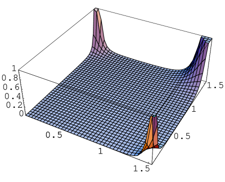
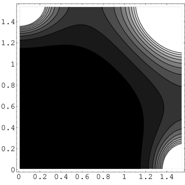
Figure 2: Left figure: The wave function of the bulk zero-mode. It is drawn for one quarter of the torus with a height rescaling by $10^{-3}$ and a chosen value of $g|q\xi_{1}|/(2\pi)=3$. Right figure: The contour presentation of the bulk zero-mode.

Comparing this mass spectrum with the one obtained in the five-dimensional case (see formula (49) of ref. [7]) we observe a qualitative difference. There, the Kaluza-Klein excitations of the bulk mode became very heavy with the cut-off $\Lambda$ and in the limit $\Lambda\rightarrow\infty$ we just retained a massless zero mode localized at a fixed point. Effectively the bulk field underwent a dimensional transmutation and became a brane field. In the present six-dimensional case such a radical effect does not happen. The zero mode bulk field shows a localization behaviour (as illustrated in Fig. 2), but the Kaluza-Klein excitations are not removed and the bulk field retains its six-dimensional nature.

5 Green-Schwarz mechanism for anomaly cancellation on the orbifold

Localized FI-tadpoles will in general imply the presence of localized anomalies. In this section, we consider the general case of local abelian and nonabelian anomalies coming from bulk as well as brane fermions. In orbifolds, consistency requires the consideration of bulk anomalies as well as local anomalies appearing at the fixed points [19, 20, 21, 22, 23, 24, 25, 26, 27]. The zero mode of a bulk fermion contributes to the local anomalies with equal distribution at the fixed points and a brane fermion also leads to local anomalies at its fixed point. If eq. (57) is fulfilled, we see that the $U(1)$ mixed gravitational anomalies are globally vanishing for the supersymmetric vacuum. On the other hand, in general, it is not guaranteed that the $U(1)$ mixed gauge anomalies are also globally cancelled. In this section, we first give a general review on the anomaly cancellation on $d=6$ orbifolds from the field theory point of view. Then, we show how a generalized Green-Schwarz (GS) mechanism [28] with various antisymmetric tensor fields can lead to a cancellation of both bulk and local anomalies. In view of applications towards the heterotic string we explicitely work out the conditions on the model where only one two-form field strength cancels all anomalies.

The discussion in this paper is, of course, not restricted to the consideration of the pure six-dimensional case, but should also be understood as a building block towards the ten-dimensional picture. It might thus occur that there are more sectors of different dimensions which should be put together to obtain the full model. In such a case formulae like (57) might have to be fulfilled only globally and not separately for each sector. For the sake of simplicity we here restrict our discussion to the six-dimensional case and deduce the conditions for anomaly cancellation in that scheme. The generalization to more complex systems should then be straightforward.

So let us first consider the bulk anomaly. The factorizable $d=6$ bulk anomaly comes from two different anomaly polynomials

$$I^{(1)}_{8} = X_{4}{\tilde{X}}_{4},$$ (90)

$$I^{(2)}_{8} = X_{2}X_{6},$$ (91)

where all forms on the right-hand sides are Casimir invariants containing the gravitational ($R$) and/or gauge field strengths ($F$). The first one contains only second order Casimir invariants while the second one involves cubic anomalies with $U(1)$. In principle, the bulk anomalies of the types $I^{(1)}_{8}$ and $I^{(2)}_{8}$ can be cancelled by a $d=6$ GS term with a bulk 2-form and a bulk 4-form, respectively. However, the existence of the $I^{(2)}_{8}$ anomaly renders the $U(1)$ massive due to the nonzero six-dimensional dual axion coupling with the $U(1)$, irrespective of the absence of the four-dimensional anomaly.

On the orbifold, there also appear local anomalies at the fixed points which take the forms as follows

$$I^{(1)}_{6} = Y_{2}Y_{4},$$ (92)

$$I^{(2)}_{6} = Y_{6},$$ (93)

where $Y_{2}$ denotes the field strength of the bulk $U(1)$ and $Y_{4},Y_{6}$ are other Casimir invariants. Thus the local abelian and non-abelian anomalies somehow modify $I^{(1)}_{8}$ and $I^{(2)}_{8}$, respectively.

It has been already shown that the local reducible $U(1)$ anomalies of type $I^{(1)}_{6}$ can be cancelled by the GS mechanism with brane 2-forms [23, 29] or a bulk two-form [9, 27], irrespectively of whether they are globally vanishing or not. For the $U(1)$ anomaly of type $I_{6}=\sum_{I}c_{I}FY_{4}|_{z_{I}}$, with $c_{I}$ being arbitrary numbers, the relevant GS Lagrangian with four brane axions becomes

$$S_{GS}=\int\sum_{I}\bigg{[}-\frac{1}{2}|da^{I}-A|^{2}-c_{I}a_{I}Y_{4}\bigg{]}\delta^{2}(z-z_{I})d^{2}z$$ (94)

where $F=dA$ is the $U(1)$ field strength and the axion $a_{I}$ at each fixed point transforms as $\delta a_{I}=\Lambda(z_{I})$ under the gauge transformation, $\delta A=d\Lambda$. In this case, independently of whether $\sum_{I}c_{I}=0$ or not, it can be seen that nonzero mass terms for $U(1)$ appear due to the local axion couplings [23, 29].

On the other hand, the local irreducible anomalies of type $I^{(2)}_{6}$, which contain the local $U(1)^{3}$ and non-abelian anomalies, can be cancelled by the GS mechanism with a bulk four-form [23, 27]. For the $U(1)$ anomaly of type $I_{6}=\sum_{I}c^{\prime}_{I}F^{3}|_{z_{I}}$, with $c^{\prime}_{I}$ being numbers satisfying $\sum_{I}c^{\prime}_{I}=0$, the relevant GS Lagrangian with one bulk four-form becomes

$$S_{GS} = \int-\frac{1}{2}|dC_{4}-Y_{5}|^{2}-\sum_{I}c^{\prime}_{I}C_{4}\delta^{2}(z-z_{I})d^{2}z$$ (95)

$$= \int\eta Y_{5}$$

where $C_{4}$ is integrated out in the last line and the one-form $\eta$ is defined as

$$d\eta=\sum_{I}c^{\prime}_{I}\delta^{2}(z-z_{I}).$$ (96)

Likewise, note that $Y_{6}=dF^{3}$, and $\delta C_{4}=Y^{1}_{4}$ with $\delta Y_{5}=dY^{1}_{4}$ under the gauge transformation. In this case, the GS mechanism involving the bulk four-form field is valid only for globally vanishing local anomalies because the bulk four-form appears only as massive KK modes in the four-dimensional effective field theory [23, 27]. Therefore, if local $U(1)^{3}$ anomalies are not reducible, there should be no integrated $U(1)^{3}$ anomaly in our model.

In the case of orbifold compactification of the heterotic string, however, the possible matter content should be much more restricted because there is only one two-form available for the GS mechanism. For instance, there would not appear either local irreducible anomalies of type $I^{(2)}_{6}$ or bulk anomalies of type $I^{(2)}_{8}$ [8, 9]. Now let us consider the simultaneous cancellation of bulk and local anomalies by the GS mechanism with only one bulk 2-form in $d=6$. The total anomaly polynomial on $T^{2}/{\bf Z}_{2}$ we are considering is

$$i(2\pi)^{3}I_{8}=\frac{1}{2}X_{4}{\tilde{X}}_{4}+i(2\pi)^{3}\sum_{I}(\frac{1}{4}I_{6}|_{r_{B}}+I_{6}|_{r_{I}})\delta^{2}(z-z_{I})d^{2}z$$ (97)

where

$$X_{4} = {\rm tr}R^{2}-\sum_{A}\alpha^{(1)}_{A}{\rm tr}_{F}F^{2}_{A},$$ (98)

$${\tilde{X}}_{4} = \frac{1}{16}({\rm tr}R^{2}-\sum_{A}\alpha^{(2)}_{A}{\rm tr}_{F}F^{2}_{A}),$$ (99)

and $I_{6}|_{r}$ denotes the four-dimensional anomaly polynomial for the bulk (brane) fermion in the representation $r=r_{B(I)}$ as

$$i(2\pi)^{3}I_{6}|_{r}=-\frac{1}{48}{\rm tr}_{r}F{\rm tr}R^{2}+\frac{1}{6}{\rm tr}_{r}F^{3}+\frac{1}{2}{\rm tr}_{r}(FF^{2}_{A}).$$ (100)

Here ${\rm tr}_{F}$ means the trace for the fundamental representation and $\alpha^{(1)}_{A}$ is given as $\alpha^{(1)}_{A}=\frac{1}{l_{A}(F)}$ for groups realized at level 1 Kac-Moody algebras [18] where $l_{A}(F)={\rm tr}_{F}(T_{A}T_{A})$ is the index of the fundamental representation of group $A$, and $\alpha^{(2)}_{A}$ depend on the matter representations [18]. Moreover, we note that the factor $\frac{1}{2}$ in the bulk anomaly comes from the reduction of the fundamental region on $T^{2}/{\bf Z}_{2}$ and the factor $\frac{1}{4}$ in the local anomaly comes from the number of fixed points. $F$ and $F_{A}$ are the abelian and non-abelian gauge field strengths.

In order for the Green-Schwarz mechanism with one bulk two-form to work for the anomaly cancellation, we need the universal relation between abelian anomalies at each fixed point as

$$\frac{1}{48}{\rm tr}Q_{I}=\frac{1}{6}{\rm tr}Q^{3}_{I}=\frac{1}{2}{\rm tr}(l_{A}(r)Q_{I}),$$ (101)

where ${\rm tr}Q_{I}=\frac{1}{4}{\rm tr}(q)+{\rm tr}(q_{I})$ and $l_{A}(r)$ is the index of representation $r$ under the gauge group $A$. In this case, other global abelian anomalies are also vanishing due to $\sum_{I}{\rm tr}Q_{I}=0$ from eq. (57). That is to say, the $d=4$ anomaly polynomial (100) becomes reducible at each fixed point as

$$I_{6}|_{r}=\alpha(FX_{4})|_{r},$$ (102)

with $\alpha=\frac{i}{(2\pi)^{3}}\frac{1}{48}$. Then, the total $d=6$ anomalies are given by

$${\cal A}_{6}=\int I^{1}_{6}+\sum_{I}I^{1}_{4}|_{I}\delta^{2}(z-z_{I})d^{2}z,$$ (103)

where $I^{1}_{6}$ and $I^{1}_{4}$ are descendents of the bulk and local anomaly polynomials, respectively.

The Green-Schwarz Lagrangian with one two-form is

$$S_{GS} = \int-\frac{1}{2}*(dB-X_{3})(dB-X_{3})$$ (104)

$$- \bigg{(}\frac{-i}{2(2\pi)^{3}}{\tilde{X}}_{3}+\sum_{I}\alpha(\frac{1}{4}A|_{r_{B}}+A|_{r_{I}})\delta^{2}(z-z_{I})d^{2}z\bigg{)}dB$$

$$+ \bigg{(}\beta{\tilde{X}}_{3}+\sum_{I}\beta_{I}(\frac{1}{4}A|_{r_{B}}+A|_{r_{I}})\delta^{2}(z-z_{I})d^{2}z\bigg{)}X_{3}.$$

Note that $X_{3}$ and ${\tilde{X}}_{3}$ are defined from $X_{4}=dX_{3}$ and ${\tilde{X}}_{4}=d{\tilde{X}}_{3}$, and $\delta X_{3}=dX^{1}_{2}$ and $\delta{\tilde{X}}_{3}=d{\tilde{X}}^{1}_{2}$ under the gauge transformation. Thus, the modified kinetic term in eq. (104) requires that $\delta B=X^{1}_{2}$ under the gauge transformation. Therefore, we find that the bulk and local anomalies in eq. (103) are cancelled by the variation of the above Green-Schwarz action with $\beta=\frac{-i}{4(2\pi)^{3}}$ and $\beta_{I}=\frac{1}{3}\alpha$.

Before closing this section, let us make a remark on the axion gauge coupling at the fixed points. From the second line in eq. (104), we find that the two-form field generically has different couplings with the $U(1)$ gauge potentials at different fixed points:

$$-\int\sum_{I}\alpha(\frac{1}{4}A|_{r_{B}}+A|_{r_{I}})\delta^{2}(z-z_{I})d^{2}zdB$$ (105)

$$= -\sum_{I}\alpha(\frac{1}{4}{\rm tr}(q)+{\rm tr}(q_{I}))\int d^{4}xA_{a}(x,z_{I})\partial^{a}b(x,z_{I})$$

where under the local duality transformation of the two-form, $b(x,z_{I})$ is considered as a brane projection of the ${\bf Z}_{2}$ even $B_{56}$ as the following

$$\partial_{[a}B_{bc]}(x,z_{I}) = \varepsilon_{abcd56}\,\partial^{[d}B^{56]}(x,z_{I})$$ (106)

$$\equiv \varepsilon_{abcd}\,\partial^{d}b(x,z_{I}).$$

Therefore, plugging into eq. (105) the zero modes of $A_{a}(x,z)$ and $b(x,z)$ which are constant in the bulk, the effective axion coupling becomes vanishing due to eq. (57) after the sum of the local axion gauge couplings. Consequently, we find that the local axion gauge couplings incorporated for the local anomaly cancellation do not break the $U(1)$.

6 Concluding remarks

The consideration of higher dimensional brane world schemes leads to fascinating possibilities to extend the standard model of particle physics. The most promising starting point is provided by superstring theory in $d=10$ or M-theory in $d=11$, with six or seven compactified dimensions, respectively. In the framework of $d=10$ supersymmetric string theories, extra space dimensions typically appear in complex pairs. Such theories contain matter fields on branes of various dimensionalities. The profile of the higher dimensional bulk fields in the presence of (lower dimensional) brane fields is of particular importance for the phenomenological properties of a given scheme. Earlier studies in the co-dimension 1 case revealed a specific localization phenomenon in the presence of localized FI-tadpoles, where a ($d=5$) bulk field dimensionally transmuted to a ($d=4$) brane field. In this paper we examined the more complicated case of co-dimension 2 in the framework of a supersymmetric orbifold theory in 6 space-time dimensions. Because of the holomorphic structure of the one complex (= two real) extra dimensions we were able to compute the Kaluza-Klein mass spectrum and the wave function of the zero-mode bulk field explicitly. The key ansatz is given in equation (60), where the holomorphic structure is transparent. Again we find a localization phenomenon of the bulk zero mode (see equation (65) and for illustration figure 2), but the situation differs from the co-dimension 1 case, as the bulk field retains its six-dimensional nature. The spectrum of massive modes equation (89) is equivalent to a spectrum in the presence of a constant Wilson line.

The co-dimension 2 case should be relevant for the discussion of those compactified superstring theories in $d=10$, where we deal in general with 3 complex extra dimensions and the presence of 3-branes ($d=4$) and 5-branes ($d=6$). In addition the co-dimension 1 case could find its application in $d=11$ M-theory and/or string theories that contain 3-branes and 6-branes of $d=7$. The potential problem of localized gauge or gravitational anomalies is cured with the help of a generalized Green-Schwarz mechanism.

Appendix A Notations and Conventions

Our conventions are six-dimensional generalizations of the ones used in [30, 11]. The metric is $\eta_{AB}=diag(+-----)$; $A,B=0,1,2,3,5,6$ are six-dimensional indices and $a,b=0,\ldots,3$ are four-dimensional ones.

Our gamma-matrices are antisymmetrized with strength one. As always in even dimensional spacetimes, one can introduce a chirality operator which is defined in the six-dimensional case by (with $\varepsilon^{012356}=+1$)

$$\Gamma^{7}=\frac{1}{6!}\varepsilon^{A_{1}\ldots A_{6}}\Gamma_{A_{1}\ldots A_{6}}.$$ (107)

An explicit representation for the gamma-matrices is

$$\Gamma^{a}=\tau^{1}\otimes\gamma^{a},\qquad\Gamma^{5}=\tau^{1}\otimes\gamma^{5},\qquad\Gamma^{6}=-i\tau^{2}\otimes\mathord{\!\leavevmode\hbox{ \begin{picture}(0.6,0.7)\put(0.0,0.0){\line(1,0){0.5}} \put(0.15,0.0){\line(0,1){0.7}} \put(0.35,0.0){\line(0,1){0.8}} \put(0.3,0.8){\rule{0.5pt}{0.5pt}}\put(0.26,0.78){\rule{0.5pt}{0.5pt}}\put(0.22,0.76){\rule{0.5pt}{0.5pt}}\put(0.18,0.74){\rule{0.5pt}{0.5pt}}\put(0.14,0.72){\rule{0.5pt}{0.5pt}}\put(0.1,0.7){\rule{0.5pt}{0.5pt}}\put(0.06,0.68){\rule{0.5pt}{0.5pt}}\put(0.02,0.66){\rule{0.5pt}{0.5pt}}\put(-0.02,0.64){\rule{0.5pt}{0.5pt}}\put(-0.06,0.62){\rule{0.5pt}{0.5pt}}\put(-0.1,0.6){\rule{0.5pt}{0.5pt}}\put(-0.14,0.58){\rule{0.5pt}{0.5pt}} \end{picture}}}_{4},$$ (108)

where $\gamma^{a}$ and $\gamma^{5}$ are the standard four-dimensional gamma matrices, with

$$\gamma^{5}=-\gamma^{0}\gamma^{1}\gamma^{2}\gamma^{3}.$$ (109)

In this basis, the six-dimensional chirality operator is diagonal:

$$\Gamma^{7}=-\tau^{3}\otimes\mathord{\!\leavevmode\hbox{ \begin{picture}(0.6,0.7)\put(0.0,0.0){\line(1,0){0.5}} \put(0.15,0.0){\line(0,1){0.7}} \put(0.35,0.0){\line(0,1){0.8}} \put(0.3,0.8){\rule{0.5pt}{0.5pt}}\put(0.26,0.78){\rule{0.5pt}{0.5pt}}\put(0.22,0.76){\rule{0.5pt}{0.5pt}}\put(0.18,0.74){\rule{0.5pt}{0.5pt}}\put(0.14,0.72){\rule{0.5pt}{0.5pt}}\put(0.1,0.7){\rule{0.5pt}{0.5pt}}\put(0.06,0.68){\rule{0.5pt}{0.5pt}}\put(0.02,0.66){\rule{0.5pt}{0.5pt}}\put(-0.02,0.64){\rule{0.5pt}{0.5pt}}\put(-0.06,0.62){\rule{0.5pt}{0.5pt}}\put(-0.1,0.6){\rule{0.5pt}{0.5pt}}\put(-0.14,0.58){\rule{0.5pt}{0.5pt}} \end{picture}}}_{4}.$$ (110)

The charge conjugation is then

$$C=-i\tau^{2}\otimes{\cal C},$$ (111)

where $\cal C$ is the five-dimensional charge conjugation.

Spinors carry an $SU(2)_{\cal R}$ index $i=1,2$. One can impose a symplectic Majorana condition

$$\bar{\psi}_{i}\equiv(\psi^{i})^{\dagger}\Gamma^{0}=\varepsilon_{ij}(\psi^{j})^{T}C,$$ (112)

where the charge conjugation matrix $C$ fulfills the following relations:

$$\Gamma_{A}^{T}=-C\Gamma_{A}C^{-1},\qquad C=C^{T},\qquad C^{\dagger}C=1.$$ (113)

Whenever possible we suppress the $SU(2)_{\cal R}$ indices. In this case the summation convention is from southwest to northeast, for example

$$\bar{\psi}\Gamma^{A}\lambda\equiv\bar{\psi}_{i}\Gamma^{A}\lambda^{i},\qquad\bar{\psi}\vec{\tau}\Gamma^{A}\lambda\equiv\bar{\psi}_{i}\Gamma^{A}\lambda^{j}(\vec{\tau})^{i}{}_{j},$$ (114)

with $(\vec{\tau})^{i}{}_{j}$ the standard Pauli matrices and the arrows denotes generically the vector representation of $SU(2)_{\cal R}$.

A fundamental and rather useful identity is

$$\bar{\psi}_{i}\Gamma^{A_{1}}\ldots\Gamma^{A_{n}}\lambda^{j}=(-1)^{n}\varepsilon_{ik}\varepsilon^{jl}\bar{\lambda}_{l}\Gamma^{A_{n}}\ldots\Gamma^{A_{1}}\psi^{k},$$ (115)

from which one easily deduces the symmetry properties of fermionic bilinears.

For four spinors $\psi,\lambda,\chi,\xi$ there are two Fierz identities possible, depending on the relative chirality of the fields:

If $\psi$ and $\xi$ have the same chirality, we have

$$(\bar{\chi}\psi)(\bar{\lambda}\xi) = -\frac{1}{8}(\bar{\chi}\xi)(\bar{\lambda}\psi)-\frac{1}{8}(\bar{\chi}\vec{\tau}\xi)(\bar{\lambda}\vec{\tau}\psi)$$ (116)

$$+ \frac{1}{16}(\bar{\chi}\Gamma_{AB}\xi)(\bar{\lambda}\Gamma^{AB}\psi)+\frac{1}{16}(\bar{\chi}\vec{\tau}\Gamma_{AB}\xi)(\bar{\lambda}\vec{\tau}\Gamma^{AB}\psi).$$

If $\psi$ and $\xi$ have opposite chirality, we have

$$(\bar{\chi}\psi)(\bar{\lambda}\xi) = -\frac{1}{8}(\bar{\chi}\Gamma_{A}\xi)(\bar{\lambda}\Gamma^{A}\psi)-\frac{1}{8}(\bar{\chi}\vec{\tau}\Gamma_{A}\xi)(\bar{\lambda}\vec{\tau}\Gamma^{A}\psi)$$ (117)

$$+ \frac{1}{48}(\bar{\chi}\Gamma_{ABC}\xi)(\bar{\lambda}\Gamma^{ABC}\psi)+\frac{1}{48}(\bar{\chi}\vec{\tau}\Gamma_{ABC}\xi)(\bar{\lambda}\vec{\tau}\Gamma^{ABC}\psi).$$

References

• [1] L. J. Dixon, J. A. Harvey, C. Vafa and E. Witten, “Strings On Orbifolds,” Nucl. Phys. B 261 (1985) 678.
• [2] P. Horava and E. Witten, “Heterotic and type I string dynamics from eleven dimensions,” Nucl. Phys. B 460 (1996) 506 [arXiv:hep-th/9510209].
• [3] L. E. Ibanez, J. Mas, H. P. Nilles and F. Quevedo, “Heterotic Strings In Symmetric And Asymmetric Orbifold Backgrounds,” Nucl. Phys. B 301 (1988) 157.
• [4] A. Font, L. E. Ibanez, H. P. Nilles and F. Quevedo, “Degenerate Orbifolds,” Nucl. Phys. B 307 (1988) 109 [Erratum-ibid. B 310 (1988) 764].
• [5] D. M. Ghilencea, S. Groot Nibbelink and H. P. Nilles, “Gauge corrections and FI-term in 5D KK theories,” Nucl. Phys. B 619 (2001) 385 [arXiv:hep-th/0108184].
• [6] S. Groot Nibbelink, H. P. Nilles and M. Olechowski, “Spontaneous localization of bulk matter fields,” Phys. Lett. B 536 (2002) 270 [arXiv:hep-th/0203055].
• [7] S. Groot Nibbelink, H. P. Nilles and M. Olechowski, “Instabilities of bulk fields and anomalies on orbifolds,” Nucl. Phys. B 640 (2002) 171 [arXiv:hep-th/0205012].
• [8] F. Gmeiner, S. Groot Nibbelink, H. P. Nilles, M. Olechowski and M. G. Walter, “Localized anomalies in heterotic orbifolds,” Nucl. Phys. B 648 (2003) 35 [arXiv:hep-th/0208146].
• [9] S. Groot Nibbelink, H. P. Nilles, M. Olechowski and M. G. Walter, “Localized tadpoles of anomalous heterotic U(1)’s,” Nucl. Phys. B 665 (2003) 236 [arXiv:hep-th/0303101].
• [10] S. G. Nibbelink, M. Hillenbach, T. Kobayashi and M. G. Walter, “Localization of heterotic anomalies on various hyper surfaces of T(6)/Z(4),” arXiv:hep-th/0308076.
• [11] M. Zucker, “Off-shell supergravity in five-dimensions and supersymmetric brane world scenarios,” Fortsch. Phys.  51 (2003) 899.
• [12] M. Zucker, “Gauged N = 2 off-shell supergravity in five dimensions,” JHEP 0008, 016 (2000) [arXiv:hep-th/9909144].
• [13] B. de Wit, P. G. Lauwers and A. Van Proeyen, “Lagrangians Of N=2 Supergravity - Matter Systems,” Nucl. Phys. B 255 (1985) 569.
• [14] T. Fujita, T. Kugo and K. Ohashi, “Off-shell formulation of supergravity on orbifold,” Prog. Theor. Phys. 106 (2001) 671 [arXiv:hep-th/0106051].
• [15] E. Bergshoeff, E. Sezgin and A. Van Proeyen, “Superconformal Tensor Calculus And Matter Couplings In Six-Dimensions,” Nucl. Phys. B 264 (1986) 653 [Erratum-ibid. B 598 (2001) 667].
• [16] E. A. Mirabelli and M. E. Peskin, “Transmission of supersymmetry breaking from a 4-dimensional boundary,” Phys. Rev. D 58 (1998) 065002 [arXiv:hep-th/9712214].
• [17] J. Polchinski, “String Theory. Vol. 1: An Introduction To The Bosonic String,”, section 7.2.
• [18] J. Erler, “Anomaly cancellation in six dimensions,” [arXiv:hep-th/9304104].
• [19] N. Arkani-Hamed, A. G. Cohen and H. Georgi, “Anomalies on orbifolds,” Phys. Lett. B 516 (2001) 395 [arXiv:hep-th/0103135].
• [20] C. A. Scrucca, M. Serone, L. Silvestrini and F. Zwirner, “Anomalies in orbifold field theories,” Phys.  Lett.  B 525 (2002) 169 [arXiv:hep-th/0110073].
• [21] L. Pilo and A. Riotto, “On anomalies in orbifold theories,” Phys.  Lett.  B 546 (2002) 135 [arXiv:hep-th/0202144].
• [22] R. Barbieri, R. Contino, P. Creminelli, R. Rattazzi and C. A. Scrucca, “Anomalies, Fayet-Iliopoulos terms and the consistency of orbifold field theories,” Phys. Lett.  B 66 (2002) 024025 [arXiv:hep-th/0203039].
• [23] C. A. Scrucca, M. Serone and M. Trapletti, “Open string models with Scherk-Schwarz SUSY breaking and localized anomalies,” Nucl. Phys.  B 635 (2002) 33 [arXiv:hep-th/0203190].
• [24] H. D. Kim, J. E. Kim and H. M. Lee, “TeV scale 5D $SU(3)_{W}$ unification and the fixed point anomaly cancellation with chiral split multiplets,” JHEP 0206 (2002) 048 [arXiv:hep-th/0204132].
• [25] T. Asaka, W. Buchmuller and L. Covi, “Bulk and brane anomalies in six dimensions,” Nucl. Phys. B 648 (2003) 231 [arXiv:hep-ph/0209144].
• [26] H. M. Lee, “Anomalies on orbifolds with gauge symmetry breaking,” [arXiv:hep-th/0211126].
• [27] G. v. Gersdorff and M. Quiros, “Localized anomalies in orbifold gauge theories,” [arXiv:hep-th/0305024].
• [28] M. B. Green and J. H. Schwarz, “Anomaly cancellation in supersymmetric $D=10$ gauge theory and superstring theory,” Phys.  Lett. B 149 (1984) 117.
• [29] I. Antoniadis, E. Kiritsis and J. Rizos, Nucl. Phys. B 637 (2002) 92 [arXiv:hep-th/0204153].
• [30] M. Zucker, “Minimal off-shell supergravity in five dimensions,” Nucl. Phys. B 570 (2000) 267 [arXiv:hep-th/9907082].