Numerical Results on the Non–Commutative $\lambda\phi^{4}$ Model

Resumé

The UV/IR mixing in the $\lambda\phi^{4}$ model on a non-commutative (NC) space leads to new predictions in perturbation theory, including Hartree–Fock type approximations. Among them there is a changed phase diagram and an unusual behavior of the correlation functions. In particular this mixing leads to a deformation of the dispersion relation. We present numerical results for these effects in $d=3$ with two NC coordinates.

1 INTRODUCTION

Field theories defined on a NC geometry are highly fashionable, in particular because they arise from a low energy limit of string theory [1].

A NC space may be defined by the non–commutativity of some of its coordinates

$$[\hat{x}_{\mu},\hat{x}_{\nu}]=i\Theta_{\mu\nu}\,\overset{\text{2d}}{=}\,i\theta\epsilon_{\mu\nu}\,.$$ (1)

For a review of NC field theories, see Ref. [2].

2 THE NC $\lambda\phi^{4}$ MODEL

The extension of actions of commutative field theories to their NC counterparts can be realized by replacing all products between fields by the star–product

$$f(x)\star g(x)=e^{\frac{1}{2}i\Theta_{\mu\nu}\frac{\partial}{\partial x_{\mu}}\frac{\partial}{\partial y_{\nu}}}f(x)g(y)|_{x=y}\,.$$ (2)

In the NC $\lambda\phi^{4}$ model this replacement leads to the action

$$S\!=\!\!\int\!d^{d}x\!\left[\frac{1}{2}\partial_{\mu}\phi\,\partial_{\mu}\phi\!+\!\frac{m^{2}}{2}\phi^{2}\!+\!\frac{\lambda}{4}\phi\star\phi\star\phi\star\phi\right]\,,$$

where only the interaction term requires the star–product.

In perturbation theory the one loop contribution to the 1 PI two point function splits into two parts coming from the planar and the non–planar graphs. The planar terms are proportional to their (UV divergent) commutative counterparts [3]. In the case of the non–planar graphs the momentum cut–off $\Lambda$ is replaced by an effective cut–off $\Lambda_{\text{eff}}$ [4],

$$\Lambda_{\text{eff}}^{2}=\frac{1}{\frac{1}{\Lambda^{2}}+\theta^{2}p^{2}}\,,$$ (3)

where $p$ denotes the incoming momentum. The cut–off $\Lambda$ may be safely send to infinity, leading to a UV finite contribution. However, the UV divergences reappear as IR divergences in the limit $p\to 0$. This mixing of UV and IR effects still causes serious problems in a perturbative treatment of NC field theories beyond one loop.

We studied the mixing of divergences non–perturbatively in the 3d model, with a commutative time direction. To avoid the (CPU) time consuming lattice version of the star–product, we mapped the system on a dimensionally reduced model [7]. Here the scalar fields $\phi(\vec{x},t)$ defined on a $N^{2}\times T$ lattice are mapped on $N\times N$ Hermitian matrices $\hat{\phi}(t)$. Their action reads

$$S[\hat{\phi}] =\vspace{-.1cm}N\textrm{Tr}\sum_{t=1}^{T}\biggl{[}\frac{1}{2}\sum_{\mu}\left(\Gamma_{\mu}\hat{\phi}(t)\,\Gamma_{\mu}^{\dagger}\!-\hat{\phi}(t)\right)^{2}$$

$$+\frac{1}{2}\left(\hat{\phi}(t\!+\!1)-\hat{\phi}(t)\right)^{2}\!\!+\!\frac{m^{2}}{2}\hat{\phi}^{2}(t)+\frac{\lambda}{4}\hat{\phi}^{4}(t)\biggl{]}\,,$$

where the twist–eaters $\Gamma_{\mu}$ are defined by

$$\Gamma_{\mu}\Gamma_{\nu}=Z^{*}_{\mu\nu}\Gamma_{\nu}\Gamma_{\mu}\,,\quad\text{where}$$ (5)

$$Z_{\mu\nu}=e^{\pi i\frac{N+1}{N}}=Z_{\nu\mu}^{*}\quad(\mu<\nu)\quad\text{is the twist.}$$

This implies $\theta=\frac{1}{\pi}Na^{2}$, where $a$ is the lattice spacing. For this action we studied the phase diagram and the dispersion relation.

3 THE PHASE DIAGRAM

Based on the momentum dependent order parameter $\langle M(k)\rangle$, with

$$M(k):=\frac{1}{NT}\max_{|\vec{p}|=k}\bigl{|}\sum_{t}\tilde{\phi}\;(\vec{p},t)\bigl{|}\,,$$ (6)

we studied the phase diagram in the $\lambda$–$m^{2}$ plane. Our results for various values of $N=T$ are shown in Fig. 1.

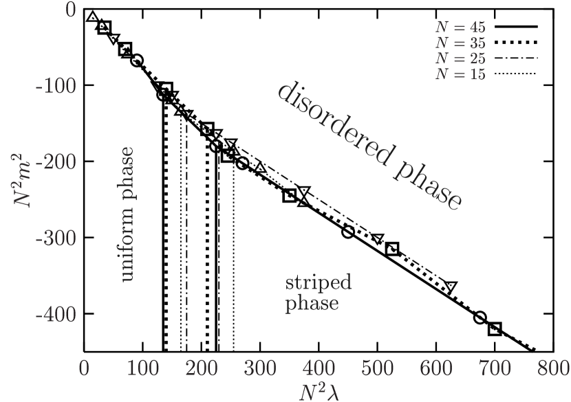
Figur 1: The phase diagram of the 3d NC $\lambda\phi^{4}$ model. The connected symbols show the separation line between disordered and ordered regime, and the vertical lines mark the transition region between uniformly ordered and striped phase.

We identify a clear separation line (connected symbols) between the disordered phase and the ordered regime. The ordered regime splits into a uniformly ordered phase and a striped phase, where the transition region is marked by two vertical lines for each value of $N$.

To illustrate the striped phase we present in Fig. 2 snapshots of single configurations, which represent the ground state in this phase in the $x_{1}$–$x_{2}$ plane at fixed time $t$

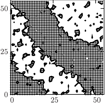
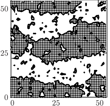
Figur 2: Snapshots of single configurations $\phi(\vec{x},t)$ at a certain time $t$, for $N=T=55$.

for $N=55$ at $\lambda=50$ and $m^{2}=-15$. The dotted areas indicate $\phi>0$ and in the blank areas $\phi$ is negative. Here we show configurations with two diagonal stripes resp. four stripes parallel to the $x_{1}$ axis. At smaller values of the coupling $\lambda$ or smaller system size $N$ we also find two stripes parallel to one of the axis [6].

These results agree qualitatively with the conjecture by Gubser and Sondhi, who predicted the occurrence of a striped phase [8]. To complete the agreement the striped phase has to survive the continuum limit, where the number of stripes should diverge, such that the width of the stripes remains finite.

4 DISPERSION RELATION

The star–product breaks explicitly the Lorentz symmetry, which leads to a deformation of the standard dispersion relation. The one loop result for this relation reads [4]

$$E(\vec{p}\,)^{2}=\vec{p}^{\,2}+M_{\text{eff}}^{2}+\xi\lambda\Lambda_{\text{eff}}\,e^{-m/\Lambda_{\text{eff}}}\,,$$ (7)

where $\Lambda_{\text{eff}}$ is defined in Eq. (3). The deformation causes a shift in the energy minimum from $\vec{p}=\vec{0}$ to non–zero momenta.

We investigated numerically the energy–momentum relation in the disordered phase. The energy $E(\vec{p})$ can be computed from the correlator

$$G(\vec{m},\tau)=\frac{1}{N^{2}T}\sum_{t}\left\langle\text{Re}\left({\tilde{\phi}^{*}(\vec{m},t)\tilde{\phi}(\vec{m},t+\tau)}\right)\right\rangle,$$

where the physical momenta are given by $\vec{p}=2\pi\,\vec{m}/N$. This correlator behaves like a cosh

$$G(\vec{m},\tau)\propto\left({e^{-E(\vec{p})\,\tau}+e^{-E(\vec{p})(T-\tau)}}\right)\,,$$ (8)

and the study of its decay allows to extract the energy. In Fig. 3 (on top) the system is close to the uniformly ordered phase transition. Here the square of the energy is linear in $\vec{p}^{\,2}$ as in a Lorentz invariant theory. Close to the striped phase (Fig. 3 below) the situation is changed. We see a clear deviation from Lorentz symmetry. The minimum of the energy is now at the lowest non–zero (lattice) momentum and thus there will be two stripes parallel to the axes in the non–uniform phase.

In Fig. 4 the results at very large coupling $\lambda$, far outside the phase diagram in Fig. 1, are shown. Now the energy minimum is shifted to larger momenta, leading to the more complicated patterns in the striped phase as in Fig. 2.

In Figs. 3 and 4 the solid lines are fits to the one loop result for the energy in Eq. (7).

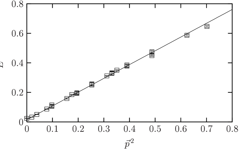
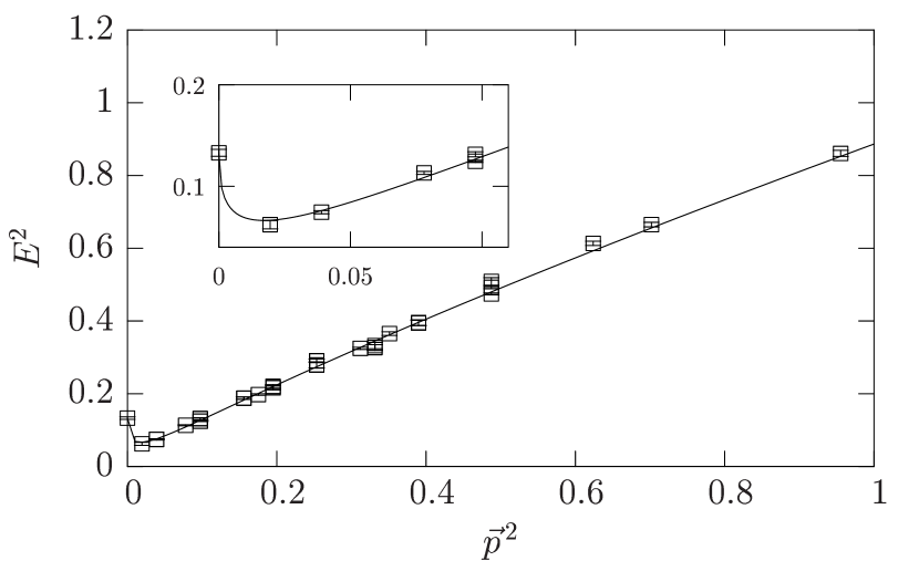
Figur 3: The dispersion relation in the disordered phase at $N=45$. Close to the uniform phase at $N^{2}\lambda=90,\,N^{2}m^{2}=-22.5$ (on top) and close to the striped phase at $N^{2}\lambda=450,\,N^{2}m^{2}=-360$ (below).

5 CONCLUSIONS

We studied numerically the effects of UV/IR mixing in the 3d NC $\lambda\phi^{4}$ model. For the phase diagram we found that the ordered regime is split into an Ising type phase for small coupling $\lambda$ and a striped phase for larger coupling. The patterns in the striped phase become more complex when $\lambda$ or the system size $N$ is increased. These results are in qualitative agreement with the conjecture of Gubser and Sondhi, if this type of stripes survives the large $N$ limit.

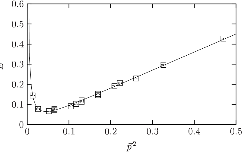
Figur 4: The dispersion relation in the disordered phase at $N=55$, $\lambda=50,\,m^{2}=-15$.

The energy–momentum relation behaves as predicted from one loop perturbation theory. This is a remarkable result, since due to the UV/IR mixing there could be strong effects from higher order calculations. Our results imply that such effects do not change the results qualitatively. However, for final conclusions one has to perform the continuum limit [9].

- [1] N. Seiberg and E. Witten, JHEP 09 (1999) 032.
- [2] R. J. Szabo, Phys. Rept. 378 (2003) 207.
- [3] T. Filk, Phys. Lett. B376 (1996) 53.
- [4] S. Minwalla, M. Van Raamsdonk and N. Seiberg, JHEP 02 (2000) 020.
- [5] J. Ambjørn and S. Catterall, Phys. Lett. B549 (2002) 253.
- [6] W. Bietenholz, F. Hofheinz and J. Nishimura, Nucl. Phys. B Proc. Suppl. 119 (2003) 941; Fortsch. Phys. 51 (2003) 745; F. Hofheinz PhD Thesis, Humboldt–Univerät zu Berlin (2003).
- [7] J. Ambjørn, Y. M. Makeenko, J. Nishimura and R. J. Szabo, JHEP 11 (1999) 029.
- [8] S. S. Gubser and S. L. Sondhi, Nucl. Phys. B605 (2001) 395.
- [9] W. Bietenholz, F. Hofheinz and J. Nishimura, in preparation.