Relationship between five-dimensional black holes and de Sitter spaces

Abstract

We study a close relationship between the topological anti-de Sitter (TAdS)-black holes and topological de Sitter (TdS) spaces including the Schwarzschild-de Sitter (SdS) black hole in five-dimensions. We show that all thermal properties of the TdS spaces can be found from those of the TAdS black holes by replacing $k$ by $-k$. Also we find that all thermal information for the cosmological horizon of the SdS black hole is obtained from either the hyperbolic-AdS black hole or the Schwarzschild-TdS space by substituting $m$ with $-m$. For this purpose we calculate thermal quantities of bulk, (Euclidean) conformal field theory (ECFT) and moving domain wall by using the A(dS)/(E)CFT correspondences. Further we compute logarithmic corrections to the Bekenstein-Hawking entropy, Cardy-Verlinde formula and Friedmann equation due to thermal fluctuations. It implies that the cosmological horizon of the TdS spaces is nothing but the event horizon of the TAdS black holes and the dS/ECFT correspondence is valid for the TdS spaces in conjunction with the AdS/CFT correspondence for the TAdS black holes.

I Introduction

Recently an accelerating universe has proposed to be a way to interpret the astronomical data of supernova[1, 2, 3]. The inflation has been employed to solve the cosmological flatness and horizon puzzles arisen in the standard cosmology. Combining the accelerating universe with the need of inflation leads to that our universe approaches de Sitter geometries in both the infinite past and the infinite future[4, 5, 6]. Hence it is important to study the nature of de Sitter (dS) space and the assumed dS/CFT correspondence[7, 8, 9]. However, some difficulties appeared in studying de Sitter space with a positive cosmological constant $\Lambda_{dS}>0$. i) There is no spatial (timelike) infinity and global timelike Killing vector. Thus it is not easy to define conserved quantities including mass, charge and angular momentum appeared in asymptotically dS space. ii) The dS solution is absent from string theories and thus we do not find a definite example to test the assumed dS/CFT correspondence. iii) It is hard to define the $S$-matrix because of the presence of the cosmological horizon.

On the other hand, we remind the reader that the cosmological horizon in dS space is very similar to the event horizon in the sense that one can define its thermodynamic quantities of a temperature and an entropy using the same way as was done for the black hole[10]. We note that the five-dimensional Schwarzschild black hole which is asymptotically flat has a negative specific heat of $C_{v}^{Sch}=-3S_{0}$ with the Bekenstein-Hawking entropy ($S_{0}$) [11]. This means that the Schwarzschild black hole is never in thermal equilibrium and it evaporates according to the Hawking radiation. But the Schwarzschild black hole could be thermal equilibrium with a radiation in a bounded box. This is because the black hole has a negative specific heat while the radiation has a positive one. The two will be in thermal equilibrium if the box is bounded. The Schwarzschild-AdS black hole belongs to this category and its specific heat takes the form of $C_{v}^{SAdS}\simeq 3S_{0}$ for large black hole. Also we note that a cosmological horizon in five-dimensional de Sitter space has a positive specific heat of $C_{v}^{dS}=3S_{0}$. This implies that the cosmological horizon in de Sitter space is rather similar to the Schwarzschild-AdS black hole than the Schwarzschild black hole. Furthermore, for large black holes including the Schwarzschild-AdS black hole, the Bekenstein-Hawking entropy receives logarithmic corrections due to thermodynamic fluctuations [12].

In this work, we establish a close relationship between the topological anti-de Sitter (TAdS)-black holes and topological de Sitter (TdS) spaces including the Schwarzschild-de Sitter (SdS) black hole in five-dimensions. We show that all thermal properties of the TdS spaces can be found from those of the TAdS black holes by replacing $k$ by $-k$. Also we find that all thermal information for the cosmological horizon of the SdS black hole is obtained from either the hyperbolic-AdS black hole or the Schwarzschild-TdS space by substituting $m$ with $-m$. For this purpose we calculate thermal quantities of bulk, (Euclidean) conformal field theory and moving domain wall by using the A(dS)/(E)CFT correspondences. Further we compute logarithmic corrections to the Bekenstein-Hawking entropy, Cardy-Verlinde formula and Friedmann equation due to thermal fluctuations. We conclude that the cosmological horizon of the TdS spaces is nothing but the event horizon of the TAdS black holes and the dS/ECFT correspondence is valid for the TdS spaces in conjunction with the AdS/CFT correspondence for the TAdS black holes. However, the dS/ECFT correspondence is not clearly realized in the SdS black hole. Hence the SdS black hole does not seems to be a toy model to study the cosmological horizon in asymptotically de Sitter space.

The organization of this paper is as follows. In section II we briefly review the bulk thermal property. Section III is devoted to studying their boundary thermal CFT. We obtain the same form of the Cardy-Verlinde formula. In order to establish the dynamical A(dS)/(E)CFT correspondence, we study the moving domain wall approach in section IV. In section V we obtain logarithmic corrections to the Cardy-Verlinde formula. Using the holographic principle, in section VI we find the modified Friedmann equations including the logarithmic terms. Finally we discuss our results in section VII.

II Bulk Thermal Property

A Topological AdS black holes

The topological AdS black holes in five-dimensional spacetimes are given by [13]

$$ds^{2}_{TAdS}=-h_{TAdS}(r)dt^{2}+\frac{1}{h_{TAdS}(r)}dr^{2}+r^{2}d\Sigma_{k}^{2},~{}~{}d\Sigma_{k}^{2}=\left[d\chi^{2}+f_{k}(\chi)^{2}(d\theta^{2}+\sin^{2}\theta d\phi^{2})\right],$$ (1)

where $d\Sigma_{k}^{2}=\gamma^{k}_{ij}dx^{i}dx^{j}$ describes the horizon geometry with a constant curvature of $6k$. $h_{TAdS}(r)$ and $f_{k}(\chi)$ are given by

$$h_{TAdS}(r)=k-\frac{m}{r^{2}}+\frac{r^{2}}{\ell^{2}},~{}~{}~{}f_{0}(\chi)=\chi,~{}f_{1}(\chi)=\sin\chi,~{}f_{-1}(\chi)=\sinh\chi.$$ (2)

Here we define $k$=1, 0, and $-1$ cases as the Schwarzschild-AdS (SAdS) black hole [14], flat-AdS (FAdS) black hole, and hyperbolic-AdS (HAdS) black hole [15], respectively. Choosing $m>0$, the only event horizon is given by

$$r_{EH}^{2}=\frac{\ell^{2}}{2}\Big{(}-k+\sqrt{k^{2}+4m/\ell^{2}}\Big{)}.$$ (3)

For $k=1$, we have both a small black hole ($r_{EH}^{2}<<\ell^{2},4m<<\ell^{2}$) with the horizon at $r=r_{EH}$, where $r_{EH}^{2}\simeq m$ and a large black hole ($r_{EH}^{2}>>\ell^{2},4m>>\ell^{2})$ with the horizon at $r=r_{EH}$ given by $r_{EH}^{2}\simeq\sqrt{m}\ell$. For $k=0$ case, one has the event horizon at $r=r_{EH}$, where $r_{EH}^{2}=\sqrt{m}\ell$. In the case of $k=-1$, for $4m<<\ell^{2}$ one has the event horizon at $r=r_{EH}$, where $r_{EH}^{2}\simeq\ell^{2}+m$ and for $4m>>\ell^{2}$ one has the event horizon at $r=r_{EH}$ given by $r_{EH}^{2}\simeq\sqrt{m}\ell$. That is, one always finds $r_{EH}^{2}>\ell^{2}$ for $k=-1$.

The relevant thermodynamic quantities: reduced mass ($m$), free energy ($F$), Bekenstein-Hawking entropy ($S_{0}$), Hawking temperature ($T_{H}$), energy (ADM mass :$E=M$), and specific heat ($C_{v}=(dE/dT)_{V}$) are given by [16]

$$m=r_{EH}^{2}\Big{(}\frac{r_{EH}^{2}}{\ell^{2}}+k\Big{)},~{}~{}F=-\frac{V_{3}r_{EH}^{2}}{16\pi G_{5}}\Big{(}\frac{r_{EH}^{2}}{\ell^{2}}-k\Big{)},~{}~{}S_{0}=\frac{V_{3}r_{EH}^{3}}{4G_{5}},~{}~{}$$ (4)

$$T_{H}=\frac{k}{2\pi r_{EH}}+\frac{r_{EH}}{\pi\ell^{2}}~{}~{}E=F+T_{H}S_{0}=\frac{3V_{3}m}{16\pi G_{5}}=M,~{}~{}C_{v}=3\frac{2r_{EH}^{2}+k\ell^{2}}{2r_{EH}^{2}-k\ell^{2}}S_{0}$$ (5)

where $G_{5}$ is the five-dimensional Newton constant. Here $V_{3(k)}=\int dx^{3}\sqrt{\gamma^{k}}$ is the volume of unit three-dimensional hypersurface. As an example, $V_{3(k=1)}=2\pi^{2}$ is the volume of a unit $S^{3}$. For simplicity we use an implicit notation of $V_{3}$ instead of $V_{3(k)}$ otherwise state. All thermodynamic quantities except for $F$ and $C_{v}$ are positive for any $k$. In the limit of $\ell\to\infty$, we recover the negative specific heat ($C_{v}^{Sch}=-3S_{s}$) of the Schwarzschild black hole. On the other hand, in the limit of $\ell\to 0$ one finds a positive value of $C_{v}^{\ell\to 0}=3S_{0}$ for the large SAdS-black hole.

B Schwarzschild de Sitter black hole

In order to find the thermal property of a black hole in asymptotically de Sitter space, we consider Schwarzschild de Sitter (SdS) black hole in five-dimensional spacetimes [17]

$$ds^{2}_{SdS}=-h_{SdS}(r)dt^{2}+\frac{1}{h_{SdS}(r)}dr^{2}+r^{2}d\Sigma_{k=1}^{2}$$ (6)

where $h_{SdS}(r)$ is given by

$$h_{SdS}(r)=1-\frac{m}{r^{2}}-\frac{r^{2}}{\ell^{2}}.$$ (7)

In the case of $m=0$, we have an exact de Sitter space with its curvature radius $\ell$. However, $m>0$ generates the SdS black hole. Here we have two horizons. The cosmological and event horizons are given by

$$r_{CH/EH}^{2}=\frac{\ell^{2}}{2}\Big{(}1\pm\sqrt{1-4m/\ell^{2}}\Big{)}.$$ (8)

We classify three cases : 1) $4m=\ell^{2}$, 2) $4m>\ell^{2}$, 3) $4m<\ell^{2}$. The case of $4m=\ell^{2}$ corresponds to the maximum black hole and the minimum cosmological horizon in asymptotically de Sitter space (that is, Nariai black hole). In this case we have $r_{EH}^{2}=r_{CH}^{2}=\ell^{2}/2=2m$. The case of $4m>\ell^{2}$ is not allowed for the black hole in de Sitter space. The case of $4m<\ell^{2}$ corresponds to a small black hole within the cosmological horizon. In this case we have the cosmological horizon at $r=r_{CH}$, where $r_{CH}^{2}\simeq\ell^{2}-m$ and the event horizon at $r=r_{EH}$ given by $r_{EH}^{2}\simeq m$. Hence we find two important relations for the SdS solution:

$$m\leq r^{2}_{EH}\leq\ell^{2}/2,~{}~{}\ell^{2}/2\leq r^{2}_{CH}\leq\ell^{2}-m$$ (9)

which means that as $m$ increases from a small value to the maximum of $m=\ell^{2}/4$, a small black hole increases up to the Nariai black hole. On the other hand the cosmological horizon decreases from a large one of $(\ell^{2}-m)$ to the minimum of $\ell^{2}/2$.

The thermodynamic quantities for two horizons are given by [18, 19]

$$m=r_{EH/CH}^{2}\Big{(}-\frac{r_{EH/CH}^{2}}{\ell^{2}}+1\Big{)},~{}~{}F_{EH/CH}=\pm\frac{V_{3}r_{EH/CH}^{2}}{16\pi G_{5}}\Big{(}\frac{r_{EH}^{2}}{\ell^{2}}+1\Big{)},~{}~{}S_{0}=\frac{V_{3}r_{EH/CH}^{3}}{4G_{5}},~{}~{}$$ (10)

$$T_{H}^{EH/CH}=\pm\frac{1}{2\pi r_{EH/CH}}\mp\frac{r_{EH/CH}}{\pi\ell^{2}},~{}~{}E=F_{EH/CH}+T_{H}^{EH/CH}S_{0}=\pm\frac{3V_{3}m}{16\pi G_{5}},$$ (11)

$$C_{v}^{EH/CH}=3\frac{2r_{EH/CH}^{2}-\ell^{2}}{2r_{EH/CH}^{2}+\ell^{2}}S_{0},$$ (12)

where $V_{3}$ denotes the volume of a unit three-dimensional sphere : $V_{3(k=1)}$. In the limit of $\ell\to\infty$, we recover the negative specific heat ($C_{v}^{Sch}=-3S_{s}$) of the Schwarzschild black hole. Considering Eqs.(9) and (10), all quantities except for $F_{CH},~{}E_{CH},~{}C_{v}^{EH}$ belong positive. On the other hand, in the limit of $\ell\to 0$ one finds a positive value of $C_{v}^{dS}=3S_{0}$ for the exact de Sitter space.

C Topological de Sitter space

The topological de Sitter (TdS) solution was originally introduced to check the mass bound conjecture in de Sitter space: any asymptotically de Sitter space with the mass greater than exact de Sitter space has a cosmological singularity [8]. For our purpose, we consider the topological de Sitter solution in five-dimensional spacetimes

$$ds^{2}_{TdS}=-h_{TdS}(r)dt^{2}+\frac{1}{h_{TdS}(r)}dr^{2}+r^{2}d\Sigma_{k}^{2},$$ (13)

where $h_{TdS}(r)$ is given by

$$h_{TdS}(r)=k+\frac{m}{r^{2}}-\frac{r^{2}}{\ell^{2}}.$$ (14)

Requiring $m>0$, the black hole disappears and instead a naked singularity occurs at $r=0$. Here we define $k=1,0,-1$ cases as the Schwarzschild-topological de Sitter (STdS) space, flat-topological de Sitter (FTdS) space, and hyperbolic–topological de Sitter (HTdS) space. In the case of $k=1,m=0$, we have an exact de Sitter space with its curvature radius $\ell$. However, $m>0$ generates the topological de Sitter spaces. The only cosmological horizon exists as

$$r_{CH}^{2}=\frac{\ell^{2}}{2}\Big{(}k+\sqrt{k^{2}+4m/\ell^{2}}\Big{)}.$$ (15)

For $k=-1$ case we have both a small cosmological horizon ($r_{CH}^{2}<<\ell^{2},4m<<\ell^{2}$) with the horizon at $r=r_{CH}$, where $r_{CH}^{2}\simeq m$ and a large cosmological horizon ($r_{CH}^{2}>>\ell^{2},4m>>\ell^{2})$ with the horizon at $r=r_{CH}$ given by $r_{CH}^{2}\simeq\sqrt{m}\ell$. For $k=0$ case, one has the cosmological horizon at $r=r_{CH}$, where $r_{CH}^{2}=\sqrt{m}\ell$. In the case of $k=1$, for $4m<<\ell^{2}$ one has the cosmological horizon at $r=r_{CH}$, where $r_{CH}^{2}\simeq\ell^{2}+m$ and for $4m>>\ell^{2}$, one has the cosmological horizon at $r=r_{CH}$, where $r_{CH}^{2}\simeq\sqrt{m}\ell$. Here we have $r_{CH}^{2}>\ell^{2}$ for $k=1$ case.

The thermodynamic quantities for the cosmological horizon are calculated as [17, 20]

$$m=r_{CH}^{2}\Big{(}\frac{r_{CH}^{2}}{\ell^{2}}-k\Big{)},~{}~{}F=-\frac{V_{3}r_{CH}^{2}}{16\pi G_{5}}\Big{(}\frac{r_{CH}^{2}}{\ell^{2}}+k\Big{)},~{}~{}S_{0}=\frac{V_{3}r_{CH}^{3}}{4G_{5}},~{}~{}$$ (16)

$$T_{H}=-\frac{k}{2\pi r_{CH}}+\frac{r_{CH}}{\pi\ell^{2}},~{}~{}E=F+T_{H}S=\frac{3V_{3}m}{16\pi G_{5}}=M,~{}~{}C_{v}=3\frac{2r_{CH}^{2}-k\ell^{2}}{2r_{CH}^{2}+k\ell^{2}}S_{0},$$ (17)

where $V_{3}$ is the volume of a unit three-dimensional hypersurface :$V_{3(k)}$. All thermal quantities except for $F$ and $C_{v}$ are positive ones. It is found from Eqs.(4), (10) and (16) that all thermodynamic results of the TdS solution can be recovered from those of the TAdS solution by replacing $k$ by $-k$. Also we find that all thermal information for the cosmological horizon of the SdS black hole is obtained from either the HAdS black hole or the STdS space by substituting $m$ with $-m$. However we note that for the same $m,\ell$, thermal quantities of the TdS case with $k$ are not precisely equal to those of the TAdS case with $-k$ because of $V_{3(k=\pm 1)}\not=V_{3(k=\mp 1)}$. Also thermal quantities of the CSdS with $V_{3(k=1)}$ is not exactly the same as in the HAdS case with $V_{3(k=-1)}$. In this sense we use a notation of $\simeq$ in TABLE.

III Boundary CFT and Cardy-Verlinde formula

TABLE I.: Summary of bulk specific heats, boundary (E)CFT energy and Casimir energy for 5D TAdS black holes, TdS spaces and SdS black hole. In the moving domain wall approach, the energy density term in Friedmann equation is included for comparison with the boundary (E)CFT energy.

thermodynamical system	$C_{v}$	$E_{4}/\rho_{(E)CFT}/E_{c}$
HAdS	+	+/+/$-$
FAdS	+($3S_{0}$)	+/+/0
SAdS	+ if $r^{2}_{EH}>\ell^{2}/2$	+/+/+
STdS($\simeq$ HAdS)	+	+/+/$-$
FTdS($\simeq$ FAdS)	+ ($3S_{0}$)	+/+/$0$
HTdS($\simeq$ SAdS)	+ if $r^{2}_{CH}>\ell^{2}/2$	+/+/+
ESdS	$-$	+/$-$/+
CSdS($\simeq$ HAdS, STdS if $m\to-m$)	+	$-/-/-$

The holographic principle means that the number of degrees of freedom associated with the bulk gravitational dynamics is determined by its boundary spacetime. The AdS/CFT correspondence represents a realization of this principle [21]. For a strongly coupled CFT with its AdS dual, one obtains the Cardy-Verlinde formula [22]. Indeed this formula holds for various kinds of asymptotically AdS spacetimes including the TAdS black holes [15]. Also it holds for asymptotically de Sitter spacetimes including the SdS black hole and TdS spaces [17]. The boundary spacetimes for the (E)CFT are defined through the A(dS)/CFT correspondences [23]

$$ds^{2}_{CFT}=\lim_{r\to\infty}\frac{R^{2}}{r^{2}}ds^{2}_{TAdS}=-\frac{R^{2}}{\ell^{2}}dt^{2}+R^{2}d\Sigma^{2}_{k},$$ (18)

$$ds^{2}_{ECFT}=\lim_{r\to\infty}\frac{R^{2}}{r^{2}}ds^{2}_{SdS}=\frac{R^{2}}{\ell^{2}}dt^{2}+R^{2}d\Sigma^{2}_{k=1},$$ (19)

$$ds^{2}_{ECFT}=\lim_{r\to\infty}\frac{R^{2}}{r^{2}}ds^{2}_{TdS}=\frac{R^{2}}{\ell^{2}}dt^{2}+R^{2}d\Sigma^{2}_{k}.$$ (20)

From the above, the relation between the five-dimensional bulk and four-dimensional boundary quantities is given by $E_{4}=(\ell/R)E,~{}T=(\ell/R)T_{H}$ where $R$ satisfies $T>1/R$ but one has the same entropy : $S_{4}=S_{0}$. We note that the boundary physics is described by the CFT-radiation matter with the equation of state: $p=E_{4}/3V_{3}$. Then the Casimir energy is given by $E_{c}=3(E_{4}+pV_{3}-TS_{0})$. We obtain the boundary thermal quantities

$$E_{4}^{TAdS}=\frac{3V_{3}m\ell}{16\pi G_{5}R},~{}~{}T^{TAdS}=\frac{k\ell}{2\pi r_{EH}R}+\frac{r_{EH}}{\pi\ell R},~{}~{}E_{c}^{TAdS}=k\frac{3\ell r_{EH}^{2}V_{3}}{8\pi G_{5}R},$$ (21)

$$E_{4}^{ESdS/CSdS}=\pm\frac{3V_{3}m\ell}{16\pi G_{5}R},~{}~{}T^{ESdS/CSdS}=\pm\frac{\ell}{2\pi r_{EH/CH}R}\mp\frac{r_{EH/CH}}{\pi\ell R},$$ (22)

$$E_{c}^{ESdS/CSdS}=\pm\frac{3\ell r_{EH/CH}^{2}V_{3}}{8\pi G_{5}R},$$ (23)

$$E_{4}^{TdS}=\frac{3V_{3}m\ell}{16\pi G_{5}R},T^{TdS}=-\frac{k\ell}{2\pi r_{CH}R}+\frac{r_{CH}}{\pi\ell R},~{}~{}~{}~{}E_{c}^{TdS}=-k\frac{3\ell r_{CH}^{2}V_{3}}{8\pi G_{5}R},$$ (24)

where ESdS (CSdS) represent the event horizon (cosmological horizon) of the SdS black hole. For the ESdS, the substitution rule of $m\to-m$ is no longer valid for deriving $E_{4}^{ESdS},E_{c}^{ESdS}$ from either the HAdS with $k=-1$ or the STdS with $k=1$. Using this expression, one finds the Cardy-Verlinde formula

$$TAdS~{}:~{}~{}S_{0CV}^{TAdS}=\frac{2\pi R}{3\sqrt{|k|}}\sqrt{|E_{c}(2E_{4}-E_{c})|},$$ (25)

$$SdS~{}:~{}~{}S_{0CV}^{SdS}=\frac{2\pi R}{3}\sqrt{|E_{c}(2E_{4}-E_{c})|},$$ (26)

$$TdS~{}:~{}~{}S_{0CV}^{TdS}=\frac{2\pi R}{3\sqrt{|k|}}\sqrt{|E_{c}(2E_{4}-E_{c})|}.$$ (27)

All static thermodynamic information is encoded in TABLE. It is shown that all thermal properties of the TdS spaces can be found from those of the TAdS black holes by replacing $k$ by $-k$. Also we find that all thermal information for the cosmological horizon of the SdS black hole is obtained from either the event horizon of the HAdS black hole or the cosmological horizon of the STdS space by substituting $m$ with $-m$. Concerning the A(dS)/CFT correspondences, we remind the reader that the boundary CFT energy ($E_{4}$) should be positive in order for it to make sense. However, one finds that $E_{4}^{CSdS}<0$ for the cosmological horizon of the SdS black hole. It suggests that the dS/CFT correspondence is not valid for this case. Also the Casimir energy ($E_{c}$) is related to the central charge of the corresponding CFT. Hence if it is negative, one may obtain a non-unitary CFT. In this sense, HAdS, STdS, and CSdS cases may be problematic. In order to understand the negative energy of $E_{4}^{CSdS}<0$, we have to study the dynamic A(dS)/(E)CFT correspondences in the next section.

IV Moving domain wall(MDW) approach

A MDW in TAdS black holes

Now we introduce the radial location of a MDW in the form of $r=a(\tau),t=t(\tau)$ parameterized by the proper time $\tau$ : $(t,r,\chi,\theta,\phi)\to(t(\tau),a(\tau),\chi,\theta,\phi)$. Then we expect that the induced metric of moving domain wall (brane) will be given by the FRW-type. Hence $\tau$ and $a(\tau)$ will imply the cosmic time and scale factor of the FRW-universe, respectively. A tangent vector (proper velocity) of this MDW

$$u=\dot{t}\frac{\partial}{\partial t}+\dot{a}\frac{\partial}{\partial a},$$ (28)

is introduced to define an embedding properly. Here overdots mean differentiation with respect to $\tau$. This is normalized to satisfy

$$u^{M}u^{N}g_{MN}=-1.$$ (29)

Given a tangent vector $u_{M}$, we need a normal 1-form directed toward to the bulk. Here we choose this as

$$n=\dot{a}dt-\dot{t}da,~{}~{}~{}n_{M}n_{N}g^{MN}=1.$$ (30)

Using either Eq.(28) with (29) or Eq.(30), we can express the proper time rate of the TAdS time $\dot{t}$ in terms of $\dot{a}$ as

$$\dot{t}=\frac{\sqrt{\dot{a}^{2}+h_{TAdS}(a)}}{h_{TAdS}(a)}.$$ (31)

The first two terms in Eq.(1) together with Eq.(31) leads to a timelike brane

$$-h_{TAdS}(r)dt^{2}+\frac{1}{h_{TAdS}(r)}dr^{2}~{}~{}\to~{}~{}-\Big{(}h_{TAdS}(a)\dot{t}^{2}-\frac{\dot{a}^{2}}{h_{TAdS}(a)}\Big{)}d\tau^{2}=-d\tau^{2}.$$ (32)

Then the 4D induced line element is

$$ds^{2}_{4TAdS} =-d\tau^{2}+a(\tau)^{2}d\Sigma^{2}_{k}$$ (34)

$$\equiv h_{\mu\nu}dx^{\mu}dx^{\nu},$$

where we use the Greek indices only for the brane. Actually the embedding of the FRW-universe is a $2(t,r)\to 1(\tau)$-mapping. The projection tensor is given by $h_{MN}=g_{MN}-n_{M}n_{N}$ and its determinant is zero. Hence its inverse $h^{MN}$ cannot be defined. This means that the above embedding belongs to a peculiar mapping to obtain the induced metric $h_{\mu\nu}$ from the TAdS black hole spacetime $g_{MN}$ together with $n_{M}$. In addition, the extrinsic curvature is defined by

$$K_{\tau\tau}=K_{MN}u^{M}u^{N}=(h_{TAdS}(a)\dot{t})^{-1}(\ddot{a}+h_{TAdS}^{\prime}(a)/2)=\frac{\ddot{a}+h_{TAdS}^{\prime}(a)/2}{\sqrt{\dot{a}^{2}+h_{TAdS}(a)}},$$ (35)

$$K_{\chi\chi}=K_{\theta\theta}=K_{\phi\phi}=-h_{TAdS}(a)\dot{t}a=-\sqrt{\dot{a}^{2}+h_{TAdS}(a)}~{}a.$$ (36)

A localized matter on the brane implies that the extrinsic curvature jumps across the brane. This jump is described by the Israel junction condition

$$K_{\mu\nu}=-\kappa^{2}\left(T_{\mu\nu}-\frac{1}{3}T^{\lambda}_{\lambda}h_{\mu\nu}\right)$$ (37)

with $\kappa^{2}=8\pi G_{5}$. We introduce a localized stress-energy tensor on the brane as the 4D perfect fluid

$$T_{\mu\nu}=(\varrho+p)u_{\mu}u_{\nu}+p\>h_{\mu\nu}.$$ (38)

Here $\varrho=\rho+\sigma$ $(p=P-\sigma)$, where $\rho$ $(P)$ is the energy density (pressure) of the localized matter and $\sigma$ is the brane tension. In the case of $\rho=P=0$, the r.h.s. of Eq.(37) leads to a form of the Randall-Sundrum case as $-\frac{\sigma\kappa^{2}}{3}h_{\mu\nu}$. From Eq.(37), one finds the space component of the junction condition

$$\sqrt{\dot{a}^{2}+h_{TAdS}(a)}=\frac{\kappa^{2}}{3}\sigma a.$$ (39)

For a single TAdS space, we introduce the fine-tuned brane tension $\sigma=3/(\kappa^{2}\ell)$ to obtain a critical brane. Then the above equation leads to

$$H^{2}_{TAdS}=-\frac{k}{a^{2}}+\frac{m_{TAdS}}{a^{4}},$$ (40)

where $H=\dot{a}/a$ is the expansion rate and $m_{TAdS}$ is given in Eq.(4). The term of $m_{TAdS}/a^{4}$ originates from the electric (Coulomb) part of the five-dimensional Weyl tensor, $E_{00}\sim m/r^{2}$. This term behaves like a radiation[25]. Especially for the SAdS, we have $m_{TAdS}=16\pi G_{5}M_{TAdS}/3V_{3},~{}M_{TAdS}=a\tilde{E}_{TAdS}/\ell,V=a^{3}V_{3},G_{5}=\ell G_{4}/2$. Then one finds a CFT-radiation dominated universe

$$H^{2}_{SAdS}=-\frac{1}{a^{2}}+\frac{8\pi G_{4}}{3}\rho_{CFT},~{}~{}~{}\rho_{CFT}=\frac{\tilde{E}_{TAdS}}{V}.$$ (41)

The equation (39) is well-defined even at $a=r_{EH}$. Thus Eq.(39) leads to $H^{2}_{TAdS}=1/\ell^{2}$ when the MDW crosses the event horizon of the TAdS black hole spaces.

B MDW in SdS black hole

As is shown in the section III, to obtain a spacelike MDW with Euclidean signature in the SdS background we have to use a different mapping. The first two terms in Eq.(6) together with $u^{M}u^{N}g_{MN}=1;~{}n^{M}n^{N}g_{MN}=-1$ leads to a spacelike brane

$$-h_{SdS}(r)dt^{2}+\frac{1}{h_{SdS}(r)}dr^{2}~{}~{}\to~{}~{}-\Big{(}h_{SdS}(a)\dot{t}^{2}-\frac{\dot{a}^{2}}{h_{SdS}(a)}\Big{)}d\tau^{2}=d\tau^{2}.$$ (42)

Then the 4D induced line element is

$$ds^{2}_{4SdS}=d\tau^{2}+a(\tau)^{2}d\Sigma^{2}_{k=1}.$$ (43)

The Israel junction condition leads to

$$\sqrt{\dot{a}^{2}-h_{SdS}(a)}=\frac{\kappa^{2}}{3}\sigma a.$$ (44)

For a single SdS black hole, we choose the brane tension $\sigma=3/(\kappa^{2}\ell)$ to obtain a critical brane. Eq.(44) leads to

$$H^{2}_{SdS}=\frac{1}{a^{2}}-\frac{m_{SdS}}{a^{4}}.$$ (45)

Here we find a negative term of $-m_{SdS}/a^{4}$ where $m_{SdS}$ is defined in Eq.(10). This term behaves like an exotic radiation[26]. Further we have $m_{SdS}=16\pi G_{5}M_{SdS}/3V_{3}$ and $M_{SdS}=a\tilde{E}_{SdS}/\ell$. Then one finds an exotic ECFT-radiation dominated universe

$$H^{2}_{SdS}=\frac{1}{a^{2}}+\frac{8\pi G_{4}}{3}\rho_{eECFT},~{}~{}~{}\rho_{eECFT}=-\frac{\tilde{E}_{SdS}}{V}.$$ (46)

The equation (44) is well-defined even at $a=r_{EH/CH}$. Thus this leads to $H_{SdS}^{2}=1/\ell^{2}$ at $a=r_{EH/CH}$. We note here that a spacelike brane can cross both the event and cosmological horizons of the SdS black hole background.

C MDW in TdS spaces

Eq.(13) together with $u^{M}u^{N}g_{MN}=1;~{}n^{M}n^{N}g_{MN}=-1$ leads to a spacelike brane

$$-h_{TdS}(r)dt^{2}+\frac{1}{h_{TdS}(r)}dr^{2}~{}~{}\to~{}~{}-\Big{(}h_{TdS}(a)\dot{t}^{2}-\frac{\dot{a}^{2}}{h_{TdS}(a)}\Big{)}d\tau^{2}=d\tau^{2}.$$ (47)

Then the induced line element is

$$ds^{2}_{4TdS}=d\tau^{2}+a(\tau)^{2}d\Sigma^{2}_{k}.$$ (48)

For a single TdS space, we introduce the brane tension $\sigma=3/(\kappa^{2}\ell)$ to obtain the critical brane. The Israel junction condition of $\sqrt{\dot{a}^{2}-h_{TdS}(a)}=\frac{\kappa^{2}}{3}\sigma a$ leads to

$$H^{2}_{TdS}=\frac{k}{a^{2}}+\frac{m_{TdS}}{a^{4}}.$$ (49)

Here we find a positive term of $m_{TdS}/a^{4}$ where $m_{TdS}$ is defined at Eq.(16). This term behaves like a radiation[26]. Further we have $m_{TdS}=16\pi G_{5}M_{TdS}/3V_{3}$ and $M_{TdS}=a\tilde{E}_{TdS}/\ell$. Then one finds a CFT-radiation dominated universe

$$H^{2}_{TdS}=\frac{k}{a^{2}}+\frac{8\pi G_{4}}{3}\rho_{ECFT},~{}~{}~{}\rho_{ECFT}=\frac{\tilde{E}_{TdS}}{V}.$$ (50)

The junction condition holds even at $a=r_{CH}$. Thus this leads to $H_{TdS}^{2}=1/\ell^{2}$ at $a=r_{CH}$.

As in the static the A(dS)/(E)CFT correspondences, we find the positive energy density $\rho_{CFT}$ in the timelike brane moving in the TAdS black hole background, while we find the negative energy density $\rho_{eECFT}$ in the spacelike brane moving in the SdS black hole background. Also one finds the positive energy density $\rho_{ECFT}$ in the spacelike brane moving in the TdS space background. This means that for the five-dimensional gravity system with a cosmological constant, the dynamic A(dS)/(E)CFT correspondences are consistent with the static A(dS)/(E)CFT correspondences. The difference is that for the TAdS black hole we obtain a CFT in the timelike brane and for the SdS black hole and TdS space we have an ECFT in the spacelike brane. Especially, the negative energy for the cosmological horizon of the SdS black hole ($E_{4}^{CSdS}$) persists in the energy density of $\rho_{eECFT}$. Hence the cosmological horizon of the SdS black hole is still problematic in view of the dS/ECFT correspondence.

It is found from Eqs.(40), (45) and (49) that the Friedmann equation for the MDW in the TdS spaces can be found from those of the TAdS black holes by replacing $k$ by $-k$. Also we find that the Friedmann equation for the MDW in the SdS black hole is obtained from either the MDW in the HAdS black hole or the MDW in the STdS space by substituting $m$ with $-m$. The energy density term of $\rho_{(E)CFT}$ is included in TABLE to compare it with the sign of the boundary (E)CFT energy $E_{4}$. In the case of the event horizon for the SdS black hole, two are different. This shows that the dS/ECFT correspondence for the SdS black hole is not yet established.

V Logarithmic corrections due to thermal fluctuations

First we make corrections to the Bekenstein-Hawking entropy. The corrected formula takes the form[12, 11, 14]

$$S=S_{0}-\frac{1}{2}\ln C_{v}+\cdots,$$ (51)

where $C_{v}$ is the specific heat of the given system at constant volume and $S_{0}$ denotes the uncorrected Bekenstein-Hawking entropy. Here an important point is that for Eq.(51) to make sense, $C_{v}$ should be positive. As is shown in TABLE, for the FAdS black hole and FTdS solution one finds $C_{v}=3S_{0}$ without any approximation. However, other cases (HAdS and SAdS black holes, CSdS, STdS and HTdS spaces) lead to $C_{v}\simeq 3S_{0}$ when choosing large black holes ($r_{EH}^{2}>>\ell^{2}$) and large cosmological horizons ($r_{CH}^{2}>>\ell^{2}$). As far as $C_{v}\simeq 3S_{0}$ is guaranteed, the logarithmic correction to the Bekenstein-Hawking entropy is given by

$$S^{TAdS,CSdS,TdS}=S_{0}-\frac{1}{2}\ln S_{0}+\cdots.$$ (52)

Note that there is no correction to the event horizon of the SdS black hole (ESdS): $S_{EH}^{ESdS}=S_{0}^{ESdS}$. Thus we do not consider this case hereafter. Logarithmic corrections to the Cardy-Verlinde formulae are being performed by calculating the Casimir energy. These are found to be

$$E_{c}^{TAdS}=k\frac{3\ell r_{EH}^{2}V_{3}}{8\pi G_{5}R}+\frac{3}{2}T\ln S_{0},$$ (53)

$$E_{c}^{CSdS}=-\frac{3\ell r_{CH}^{2}V_{3}}{8\pi G_{5}R}+\frac{3}{2}T\ln S_{0},$$ (54)

$$E_{c}^{TdS}=-k\frac{3\ell r_{CH}^{2}V_{3}}{8\pi G_{5}R}+\frac{3}{2}T\ln S_{0}.$$ (55)

Substituting the above into the Cardy-Verlinde formulae in Eqs.(25), (26) and (27), one finds

$$TAdS~{}:~{}~{}\frac{2\pi R}{3\sqrt{|k|}}\sqrt{|E_{c}(2E_{4}-E_{c})|}\simeq S_{0}+\frac{\pi R\ell T}{2kr_{EH}^{3}}\Big{(}\frac{r_{EH}^{4}}{\ell^{2}}-kr_{EH}^{2}\Big{)}\ln S_{0},$$ (56)

$$CSdS~{}:~{}~{}\frac{2\pi R}{3}\sqrt{|E_{c}(2E_{4}-E_{c})|}\simeq S_{0}-\frac{\pi R\ell T}{2r_{CH}^{3}}\Big{(}\frac{r_{CH}^{4}}{\ell^{2}}+r_{CH}^{2}\Big{)}\ln S_{0},$$ (57)

$$TdS~{}:~{}~{}\frac{2\pi R}{3\sqrt{|k|}}\sqrt{|E_{c}(2E_{4}-E_{c})|}\simeq S_{0}-\frac{\pi R\ell T}{2kr_{CH}^{3}}\Big{(}\frac{r_{CH}^{4}}{\ell^{2}}+kr_{CH}^{2}\Big{)}\ln S_{0}.$$ (58)

All coefficients in front of $\ln S_{0}$ in the above relations are transformed into the same expression as [20]

$$\frac{\pi R\ell T}{2kr_{EH}^{3}}\Big{(}\frac{r^{4}_{EH}}{\ell^{2}}-kr_{EH}^{2}\Big{)}=\frac{(4E_{4}-E_{c})(E_{4}-E_{c})}{2(2E_{4}-E_{c})E_{c}},$$ (59)

$$-\frac{\pi R\ell T}{2r_{CH}^{3}}\Big{(}\frac{r^{4}_{CH}}{\ell^{2}}+r_{CH}^{2}\Big{)}=\frac{(4E_{4}-E_{c})(E_{4}-E_{c})}{2(2E_{4}-E_{c})E_{c}},$$ (60)

$$-\frac{\pi R\ell T}{2kr_{CH}^{3}}\Big{(}\frac{r^{4}_{CH}}{\ell^{2}}+kr_{CH}^{2}\Big{)}=\frac{(4E_{4}-E_{c})(E_{4}-E_{c})}{2(2E_{4}-E_{c})E_{c}}.$$ (61)

Finally we obtain the same form of corrections to the Cardy-Verlinde formula as

$$S^{TAdS,CSdS,TdS}_{CV}\simeq\frac{2\pi R}{3\sqrt{|k|}}\sqrt{|E_{c}(2E_{4}-E_{c})|}-\frac{(4E_{4}-3E_{c})E_{4}}{2(2E_{4}-E_{c})E_{c}}\ln\Big{(}\frac{2\pi R}{3\sqrt{|k|}}\sqrt{|E_{c}(2E_{4}-E_{c})|}\Big{)}$$ (62)

where we recover the Cardy-Verlinde formula for the cosmological horizon of the SdS black hole when $k=1$. The Cardy-Verlinde formula expresses the holography which means that the bulk thermal properties can be determined from their boundary thermal CFT. Note that after logarithmic corrections to the Cardy-Verlinde formula due to thermal fluctuation, they take still the same form. This means that there is no crucial difference between the event horizon of the TAdS black hole and the cosmological horizons of the TdS spaces and the SdS black holes.

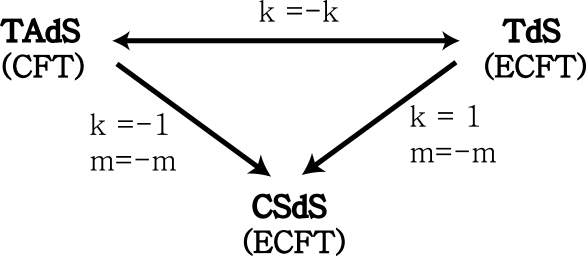
FIG. 1.: The diagram for the static relation between TAdS, TdS, and CSdS. The CFT in TAdS black hole is defined on the timelike boundary, while the ECFT in TdS spaces and CSdS black hole is defined on the spacelike boundary.

Fig.1 shows a close relationship between TAdS, TdS, and CSdS after logarithmic corrections.

VI Logarithmic corrections to the MDW

In section IV, the brane cosmology has been studied in the framework of the dynamic A(dS)/(E)CFT correspondences. The brane starts with (big bang) inside the event horizon (cosmological horizon), crosses the horizon, and expands until it reaches maximum size. And then the brane contracts, it falls the horizon again and finally disappears (big crunch). An observer in the bulk space finds two interesting moments when the brane crosses the past (future) horizon. Authors in ref.[25] showed that at these times the Friedmann equation controlling the cosmological expansion (contraction) coincides with a Cardy-Verlinde formula for the entropy of the CFT on the brane. That is, the location of the event horizon (cosmological horizon) is a holographic point. On the Cardy-Verlinde formula side, one can obtain its logarithmic correction due to thermal fluctuations of the bulk gravity system. However, it is not easy to obtain its corresponding term in the Friedmann equation. Up to now we don’t know how to embed the logarithmic term into the Friedmann equation. The only way is to use a holographic point if one assumes that the Cardy-Verlinde formula coincides the Friedmann equation when the MDW crosses the horizon of the bulk spacetime. Using the Hubble entropy of $H^{2}=\Big{(}\frac{2G_{4}}{V}\Big{)}S_{CV}^{2}$ and Eq.(62), one finds the modified relations at the holographic point

$$H^{2}_{TAdS}=\frac{1}{\ell^{2}}-\frac{2G_{4}}{V\ell}\ln S_{0}=-\frac{k}{a_{EH}^{2}}+\frac{8\pi G_{4}}{3}\rho_{CFT}-\frac{2G_{4}}{V\ell}\ln S_{0},$$ (63)

$$H^{2}_{CSdS}=\frac{1}{\ell^{2}}-\frac{2G_{4}}{V\ell}\ln S_{0}=\frac{1}{a_{CH}^{2}}+\frac{8\pi G_{4}}{3}\rho_{eECFT}-\frac{2G_{4}}{V\ell}\ln S_{0},$$ (64)

$$H^{2}_{TdS}=\frac{1}{\ell^{2}}-\frac{2G_{4}}{V\ell}\ln S_{0}=\frac{k}{a_{CH}^{2}}+\frac{8\pi G_{4}}{3}\rho_{ECFT}-\frac{2G_{4}}{V\ell}\ln S_{0}.$$ (65)

The expansion (contraction) rate at a holographic point decreases in comparison with the case without correction : $H^{2}_{TAdS,SdS,TdS}=1/\ell^{2}$. We assume to extend these relations to the modified Friedmann equations

$$H^{2}_{TAdS}=-\frac{k}{a^{2}}+\frac{8\pi G_{4}}{3}\rho_{CFT}-\frac{2G_{4}}{V\ell}\ln S_{0},$$ (66)

$$H^{2}_{CSdS}=\frac{1}{a^{2}}+\frac{8\pi G_{4}}{3}\rho_{eECFT}-\frac{2G_{4}}{V\ell}\ln S_{0},$$ (67)

$$H^{2}_{TdS}=\frac{k}{a^{2}}+\frac{8\pi G_{4}}{3}\rho_{ECFT}-\frac{2G_{4}}{V\ell}\ln S_{0}$$ (68)

which are valid for other points in the bulk background. Here $V=a^{3}V_{3}$ and $S_{0}=V_{3}a^{3}/4G_{5}$. In the absence of logarithmic corrections, the above equations reduce to Eqs.(41), (46) and (50) respectively. Let us transform the modified Friedmann equation to the conservation of energy for a point particle moving under the one-dimensional potential $V$ as

$${\dot{a}}^{2}=-k-V_{TAdS},~{}~{}V_{TAdS}=-\frac{m_{TAdS}}{a^{2}}+\frac{2G_{4}}{V_{3}\ell a}\ln\Big{(}\frac{V_{3}a^{3}}{2\ell G_{4}}\Big{)},$$ (69)

$${\dot{a}}^{2}=1-V_{CSdS},~{}~{}V_{CSdS}=\frac{m_{SdS}}{a^{2}}+\frac{2G_{4}}{V_{3}\ell a}\ln\Big{(}\frac{V_{3}a^{3}}{2\ell G_{4}}\Big{)},$$ (70)

$${\dot{a}}^{2}=k-V_{TdS},~{}~{}V_{TdS}=-\frac{m_{TdS}}{a^{2}}+\frac{2G_{4}}{V_{3}\ell a}\ln\Big{(}\frac{V_{3}a^{3}}{2\ell G_{4}}\Big{)}.$$ (71)

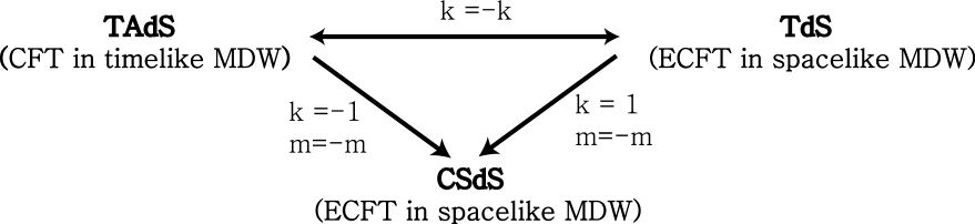
FIG. 2.: The diagram for the relation between TAdS, TdS, and CSdS. The CFT in TAdS black hole is defined on the timelike MDW, while the ECFT in TdS spaces and CSdS black hole is defined on the spacelike MDW.

Fig.2 shows a close relationship between TAdS, TdS, and CSdS after logarithmic corrections to the Friedmann equation. For the cosmological implication of logarithmic corrections, we consult ref.[16] for the TAdS and TdS cases and ref.[19] for the SdS case. The logarithmic correction ($\ln a/a$) to the timelike (spacelike) MDW under the HAdS black hole (STdS space) give us additional bouncing cosmologies without any big bang singularity, in compared with others of the big bang $\to$ big crunch. Although there exists logarithmic correction to the spacelike MDW in the SdS space, the physical interpretation is still unclear because of the presence of the exotic energy density :$\rho_{eECFT}=-\tilde{E}/V$. Finally we are not sure that these logarithmic corrections could be included after corrections to the Friedmann equations.

VII Discussion

We show that all thermal properties of the TdS spaces can be found from those of the TAdS black holes by replacing $k$ by $-k$. This means that the cosmological horizon in TdS spaces is nearly identical with the event horizon of the TAdS black holes. Also we find that all thermal information for the cosmological horizon of the SdS black hole is obtained from either the hyperbolic-AdS black hole or the Schwarzschild-TdS space by substituting $m$ with $-m$. This means that the cosmological horizon of the SdS black hole is nothing special.

Concerning the SdS black hole with the cosmological and event horizons, the dS/CFT correspondence is problematic because as is shown in TABLE, the event horizon has an exotic (negative) energy density in the Friedmann equation while the cosmological horizon has a negative CFT energy and an exotic energy density. Also the negative Casimir energy for the cosmological horizon implies the non-unitary CFT. In addition the event horizon inside the cosmological horizon has the negative specific heat, which means that it is thermodynamically unstable. Hence the SdS black hole does not seems to be a toy model to study the cosmological horizon in asymptotically de Sitter space because it has two horizons.

We suggest that the TdS spaces including a cosmological singularity are better candidates for studying thermal property for the cosmological horizon than the SdS black hole. Considering the close relationship between the TdS spaces and the TAdS black holes, the cosmological horizon is nothing but the event horizon. Also the dS/ECFT correspondence is well established for the TdS spaces in conjunction with the AdS/CFT correspondence for the TAdS black holes. However, in the wave equation approach to find the absorption cross section, two may be different because their working spaces are different (the TdS case is compact whereas the TAdS is non-compact)[28].

REFERENCES

• [1] S. Perlmutter et al.(Supernova Cosmology Project), Astrophys. J. 483, 565(1997)[astro-ph/9608192].
• [2] R. R. Caldwell, R. Dave, and P. J. Steinhard, Phys. Rev. Lett. 80, 1582(1998)[astro-ph/9708069].
• [3] P. M. Garnavich et al., Astrophys. J. 509, 74(1998)[astro-ph/9806396].
• [4] E. Witten, hep-th/0106109.
• [5] S. Hellerman, N. Kaloper, and L. Susskind, JHEP 0106, 003(2001)[hep-th/0104180].
• [6] W. Fischler, A. Kashani-Poor, R. McNees, and S. Paban, JHEP 0107, 003 (2001)[hep-th/0104181].
• [7] R. Bousso, JHEP 0011, 038 (2000)[hep-th/0010252]; R. Bousso, JHEP 0104, 035 (2001)[hep-th/0012052];
• [8] V. Balasubramanian, J. de Boer, and D. Minic, Phys. Rev. D65 (2002) 123508 [hep-th/0110108]; R. G. Cai, Y. S. Myung, and Y. Z. Zhang, Phys. Rev. D65 (2002) 084019 [hep-th/0110234]; Y. S. Myung, Mod. Phys. Lett.A16 (2001) 2353 [hep-th/0110123]; A. M. Ghezelbach and R. B. Mann, JHEP 0201 (2002) 005 [hep-th/0111217].
• [9] A. Strominger, JHEP 0110, 034 (2001)[hep-th/0106113].
• [10] G. W. Gibbons and S. W. Hawking, Phys. Rev. D15, 2738(1977).
• [11] S. Das, P. Majumdar, and R. K. Bhaduri, Class. Quant. Grav. 19 (2002) 2355 [hep-th/0111001].
• [12] R. K. Kaul and P. Majumdar, Phys. Lett. B439 (1998) 267 [gr-qc/9801080]; R. K. Kaul and P. Majumdar, Phy. Rev. Lett, 56 (2000)5255 [gr-qc/0002040]; S. Carlip, Class. Quant. Grav. 17 (2000) 4175 [gr-qc/0005017]; T. R. Govindarajan, R.K. Kaul and V. Suneeta, Class. Quant. Grav. 18 (2001) [gr-qc/0104010]; D. Birmingham and S. Sen, Phys. Rev. D63 (2001) 047501 [hep-th/0008051]; J. Jing and Mu-Lin Yan, Phys. Rev. D63 (2001) 024003 [gr-qc/0005105].
• [13] D. Birmingham, Class. Quant. Grav. 16 (1999) 1197 [hep-th/9808032].
• [14] S. Mukherji and S. S. Pal, JHEP 0205 (2002) 026 [hep-th/0205164].
• [15] R. G. Cai, Phys. Rev. D63 (2001) 124018 [hep-th/0102113].
• [16] J. E. Lidsey, S. Nojiri, S. Odintsov, and S . Ogushi, Phys. Lett. B544 (2002) 337 [hep-th/0207009].
• [17] R. G. Cai, Phys. Lett. B525 (2002) 331 [hep-th/0111093].
• [18] R. G. Cai and Y. S. Myung, Phys. Rev. D67 (2003) 124021 [hep-th/0210272].
• [19] S. Nojiri, S. Odintsov, and S. Ogushi, Int. J. Mod. Phys. A18 (2003) 3395 [hep-th/0212047];
• [20] Y. S. Myung, hep-th/0308191, to appear in Physics Letters B.
• [21] J. Maldacena, Adv. Theor. Math. Phys. 2 (1998) 231 [hep-th/9711200]; S.S Gubser, I.R. Klebanov, and A.M. Polyakov, Phys. Lett. B428 (1998) 105 [hep-th/9802109]; E. Witten, Adv. Theor. Math. Phys. 2 (1998) 253 [hep-th/9802150].
• [22] E. Verlinde, hep-th/0008140.
• [23] E. Witten, Adv. Theor. Math. Phys. 2 (1998) 505 [ hep-th/9803131].
• [24] M. R. Setare, hep-th/0308106.
• [25] I. Savonije and E. Verlinde, Phys. Lett. B507 (2001) 305 [hep-th/0102042].
• [26] Y. S. Myung, Phys. Lett. B531 (2002)1 [hep-th/0112140].
• [27] S. Shankaranarayanan, Phys. Rev. D67 (2003) 084026 [gr-qc/0301090].
• [28] Y. S. Myung, hep-th/0304231.