WMAP constraint on the P-term inflationary model

Abstract

In light of WMAP results, we examine the observational constraint on the P-term inflation. With the tunable parameter $f$, P-term inflation contains richer physics than D-term and F-term inflationary models. We find the logarithmic derivative spectral index with $n>1$ on large scales and $n<1$ on small scales in agreement to observation. We obtained a reasonable range for the choice of the gauge coupling constant $g$ in order to meet the requirements of WMAP observation and the expected number of the e-foldings. Although tuning $f$ and $g$ we can have larger values for the logarithmic derivative of the spectral index, it is not possible to satisfy all observational requirements for both, the spectral index and its logarithmic derivative at the same time.
PACS number(s): 98.80.Cq

I Introduction

One of the fundamental ideas of modern cosmology is that in its very early epoch of history our universe was dominated by the potential energy of a slowly rolling scalar field 1 2 . During such an era the scale factor grew exponentially in a very short period of time, leading to the homogeneity and isotropy of the observed universe to a high accuracy. The inflationary scenario has been supported by COBE 3 and other large scale galaxy surveys 4 . The recently released first year high precision data of the WMAP further confirmed the inflationary mechanism 5 .

There are various single-field inflationary models. Among them, non-symmetric grand unified theories which give rise to the inflationary scenario were constructed more than a decade ago. Besides the standard model, supersymmetry has been considered both as a blessing and as a curse for inflationary model building. It is a blessing, primarily because it allows one to have very flat potential, as well as to fine-tune any parameters at the tree level. Moreover it seems more natural than the non-symmetric theories. It is a curse, because during inflation one needs to consider supergravity, where usually all scalar fields have too big masses to support inflation. However it was shown that in the $N=1$ generic D-term inflation the inflaton field has superpotentials which vanish together with their first derivatives and does not acquire a Hubble scale mass term from the supergravity corrections 6 . It avoids the general problem of inflation in supergravity. In addition it was found that by properly choosing the minimal Kähler potential, the $N=1$ supersymmetric F-term inflation does not acquire the large mass term usually needed in supergravity either 7 .

Recently a new version of hybrid inflation, the “P-term inflation” has been introduced in the context of $N=2$ supersymmetry 8 . It is intriguing that once one breaks $N=2$ supersymmetry and implements the P-term inflation in $N=1$ supergravity, this scenario simultaneously leads to a new class of inflationary models, which interpolates between D-term and F-term models.

It is of interest to use the WMAP data to discriminate among the various single-field inflationary models kinney . For single-field inflation models, the relevant parameter space for distinguishing among models is defined by the scalar index $n$ and the logarithmic derivative of the scalar spectral index $dn/d(\ln k)$. In D-term inflation it was found that the spectrum is exactly flat with $n=1$ 8 . In the F-term inflation a small dependence of the spectral index on momenta was found, which is qualitatively consistent with the WMAP observation 5 . However, the variation of the spectral index in F-term inflation was claimed to be too mild compared to the observational data 9 10 . It was argued that this is due to the small Yukawa coupling constant required for sufficient inflation 10 . The motivation of the present paper is to use the WMAP data to restrain the P-term inflation parameter. In P-term inflation the contribution from supergravity has an additional parameter $f$ in the range $0<f<1$. We would like to explore how the inflationary regime and its properties depend on the value of the parameter $f$ to meet observation.

II P-term inflation model

We first review the P-term inflationary model of Kallosh and Linde 8 . The action of the $N=2$ supersymmetry is

$$L_{N=2}=L_{s,c}-g\vec{P}\vec{\zeta}$$ (1)

where $L_{s,c}$ is the bosonic part of the superconformal action consisting of the vector multiplet and a charged hypermultiplet. The second term in (1) is the Fayet-Iliopulos term. The potential of the P-term model can be given by using the symmetries of the theory in a form suitable for the $N=1$ notation,

$$V_{N=2} = 2g^{2}(|S\Phi_{+}|^{2}+|S\Phi_{-}|^{2}+|\Phi_{+}\Phi_{-}-\xi_{+}/2|^{2})$$ (2)

$$+ g^{2}/2(|\Phi_{+}|^{2}-|\Phi_{-}|^{2}-\xi_{3})^{2}$$

where $S$ is for the neutral scalar, $\Phi_{+}(\Phi_{-})$ for positively (negatively) charged scalar. $\xi$ is the triplet with $\xi=\sqrt{|\vec{\xi}|^{2}}=\sqrt{\xi_{+}\xi_{-}+(\xi_{3})^{2}},\xi_{\pm}=\xi_{1}+i\xi_{2}$. Here $g$ is the gauge coupling constant.

The P-term potential corresponds to that of an $N=1$ model

$$V=|\partial W|^{2}+g^{2}D^{2}/2$$ (3)

with a superpotential and a D-term given by

$$W=\sqrt{2}gS(\Phi_{+}\Phi_{-}-\xi_{+}/2),\quad D=|\Phi_{+}|^{2}-|\Phi_{-}|^{2}-\xi_{3}.$$ (4)

It coincides with the D-term inflation when $\xi_{+}=\xi_{-}=0$, $\xi_{3}=|\vec{\xi}|$ and $\lambda=\sqrt{2}g$. On the other hand choosing $\xi_{+}=\xi_{-}=\xi$ and $\lambda=\sqrt{2}g$, we can recover the F-term inflation model.

$N=2$ supersymmetry can be coupled to $N=1$ supergravity by choosing the minimal K$\ddot{a}$hler potential for all three chiral superfields. The $N=1$ supergravity has the K$\ddot{a}$hler potential and superpotential given by

$$K = \frac{|S|^{2}+|\Phi_{+}|^{2}+|\Phi_{-}|^{2}}{M_{p}^{2}}\quad,$$

$$W = \sqrt{2}gS(\Phi_{+}\Phi_{-}-\xi_{+}/2)\quad.$$ (5)

Using the superpotential

$$W=S\frac{\partial W}{\partial S}\quad,\quad KW=\frac{S\bar{S}}{M_{p}^{2}}\frac{\partial W}{\partial S}$$ (6)

the effective potential becomes

$$V =2g^{2}e^{|S|^{2}/M_{p}^{2}}\{|\frac{\partial W}{\partial S}|^{2}((1+\frac{S\bar{S}}{M_{p}^{2}})^{2}-3\frac{S\bar{S}}{M_{p}^{2}})$$

$$+ |S\Phi_{+}|^{2}+|S\Phi_{-}|^{2}\}+\frac{g^{2}}{2}(|\Phi_{+}|^{2}-|\Phi_{-}|^{2}-\xi_{3})^{2}.$$ (7)

After the tree level supergravity corrections, the complete potential reads

$$V =2g^{2}e^{|S|^{2}/M_{p}^{2}}\{|\Phi_{+}\Phi_{-}-\xi_{+}/2|^{2}(1-\frac{S\bar{S}}{M_{p}^{2}}+(\frac{S\bar{S}}{M_{p}^{2}})^{2})$$

$$+ |S\Phi_{+}|^{2}+|S\Phi_{-}|^{2}\}+\frac{g^{2}}{2}(|\Phi_{+}|^{2}-|\Phi_{-}|^{2}-\xi_{3})^{2}\;.$$ (8)

Adding the one-loop gauge theory corrections and considering that the inflation takes place at $\Phi_{+}=\Phi_{-}=0$, we find that the effective potential is given by the expression

$$V=\frac{g^{2}\xi^{2}}{2}[1+\frac{g^{2}}{8\pi}\ln\frac{|S^{2}|}{|S_{e}^{2}|}+f\frac{|S^{4}|}{2M_{p}^{2}}+...]\quad.$$ (9)

where $f=\frac{\xi_{1}^{2}+\xi_{2}^{2}}{\xi^{2}}$ and $0<f<1$.

The point $\Phi_{+}=\Phi_{-}=0$ should be stable during the slow roll period in order that the argument here presented be correct. That this is true follows from the fact that the second derivative of (8) with respect to $\Phi_{+}$ and $\Phi_{-}$ is positive as long as $2{\rm e}^{S^{2}/M_{p}^{2}}S^{2}>\xi_{3}$, which is necessary but can be achieved, as we also see a posteriori.

Switching to the canonically quantized fields $\phi_{\pm}=\sqrt{2}\Phi_{\pm}$ and $s=\sqrt{2}S$, the effective potential in units $M_{p}=1$ is

$$V=\frac{g^{2}\xi^{2}}{2}[1+\frac{g^{2}}{8\pi}\ln\frac{|s^{2}|}{|s_{e}^{2}|}+f\frac{|s|^{4}}{8}+...]\quad.$$ (10)

A general P-term inflation model has $0<f<1$ with the special case $f=0$ corresponding to the D-term inflation, while $f=1$ corresponds to the F-term inflation. Above, $s_{e}$ is the bifurcation point indicating the end of inflation. The second term in the potential is due to the one-loop correction and the third term to the supergravity correction.

Figure 1: Fig. 1a indicates the behavior of $V/V^{\prime}$. Figs. 1b and 1c show the behavior of slow-roll parameters for large and small scalar fields, respectively. Dashed line indicates the $\eta$ and the solid line is $\epsilon$.

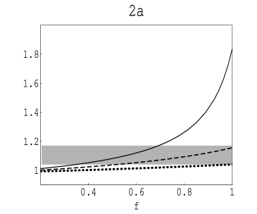
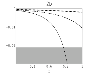
Figure 2: Dependence of the spectral index and its logarithmic derivative on $f$ for different fixed values of $g$ when $N_{k}=60$. Fig. 2a depicts $n$ and Fig.2b $dn/d\ln k$. A solid line corresponds to $g=0.11$, a dashed line to $g=0.09$, and a dotted line to $g=0.065$.

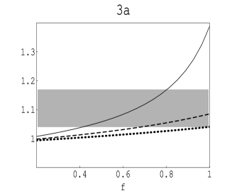
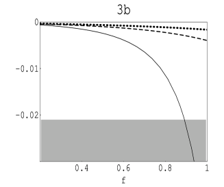
Figure 3: Dependence of the spectral index and its logarithmic derivative on $f$ for different fixed $g$ when $N_{k}=70$. Fig. 3a shows $n$ while Fig. 3b shows $dn/d\ln k$. A solid line corresponds to $g=0.09$, a dashed line to $g=0.07$ and a dotted line to $g=0.058$.

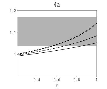
Figure 4: Dependence of the spectral index and its logarithmic derivative on $f$ for different numbers of e-foldings when $g$ is fixed. Fig. 4a corresponds to $n$ and Fig. 4b to $dn/d\ln k$. A solid line corresponds to $N_{k}=60$, a dashed line to $N_{k}=70$ and a dotted line to $N_{k}=80$.

Figure 5: Dependence of the spectral index and its logarithmic derivative on the number of e-foldings for fixed $f$ and $g$. Fig. 5a describes $n$ and Fig. 5b $dn/d\ln k$. A solid line corresponds $g=0.08,f=0.6$, a dashed line to $g=0.08,f=1$.

Figure 6: Dependence of the spectral index and its logarithmic derivative on the number of e-foldings for fixed $f$ and $g$. Fig. 6a describes $n$ and Fig. 6b $dn/d\ln k$. A solid line corresponds to $f=0.8,g=0.09$, a dashed line to $f=0.8,g=0.07$.

III The inflationary space

In a single field slow-roll inflation model with a potential $V(s)$ the amplitude of curvature perturbation is given by

$$P(k)=\frac{1}{2\pi}\frac{H^{2}(t_{k})}{|\dot{s}(t_{k})|},$$ (11)

where

$$H^{2}(t_{k})=V[s(t_{k})]/3.$$ (12)

and $t_{k}$ is the epoch where the $k$ mode left the Hubble radius during inflation 1 . As usual, the spectral index is defined by

$$n-1=\frac{d\ln|P(k)|^{2}}{d\ln k}=-6\epsilon+2\eta,$$ (13)

where

$$\epsilon=\frac{1}{2}[V^{\prime}(s)/V(s)]^{2}\quad,\quad\hbox{and}\quad\eta=V^{\prime\prime}(s)/V(s).$$ (14)

The logarithmic derivative of the spectral index is

$$\frac{dn}{d\ln k}=16\epsilon\eta-24\epsilon^{2}-2\zeta,$$ (15)

where

$$\zeta=\frac{V^{\prime\prime\prime}(s)V^{\prime}(s)}{V^{2}(s)}.$$ (16)

It has been reported that WMAP results favors purely adiabatic fluctuations with a remarkable feature that the spectral index runs from $n>1$ on a large scale to $n<1$ on a small scale. More specifically on the scale $k=0.002Mpc^{-1},n=1.10^{+0.07}_{-0.06}$ and $dn/d\ln k=-0.042^{+0.021}_{-0.020}$ 5 . It is of interest to investigate whether the P-term inflation can accommodate these observational result.

From (12), for the extremely flat potential, the scale factor of the universe is

$$a(t)=a(0)exp(g\xi t/\sqrt{6}),$$ (17)

and the approximate number of e-foldings can be written as $N=g\xi t/\sqrt{6}$.

From the potential form (10) we learnt that inflation consists of two long stages, one of them is determined by the one-loop effect and the other is determined by the supergravity corrections. Comparing the derivatives of the one-loop and supergravity correction terms in the potential ((10), we learnt that if $V^{\prime}_{1-loop}>V^{\prime}_{sugra}$, then $|s|<\sqrt{g}/(2\pi^{2})^{1/2}$. Therefore one gets $N_{1}\sim 4.5/(f^{1/2}g)$. Similarly for the $V^{\prime}_{sugra}>V^{\prime}_{1-loop}$, one has $N_{2}\sim 4.5/(f^{1/2}g)$. The total duration of inflation can be estimated by

$$N_{1}+N_{2}\sim 9/(f^{1/2}g)>N_{k},$$ (18)

where $N_{k}$ is supposed to be a reasonable number of e-foldings.

Thus we require $g<9/(N_{k}f^{1/2})$. For the F-term inflation $f=1$ and $N_{k}=60$, $g<0.15$, which is exactly the argument given in 7 .

Using (10) and (14,16), we have for the P-term inflation

$$\epsilon = \frac{1}{2}[\frac{g^{2}/(4\pi^{2}|s|)+f|s|^{3}/2}{1+g^{2}/(8\pi^{2})\ln(|s|^{2}/|s_{e}|^{2})+f|s^{4}|/8}]^{2}\quad,$$

$$\eta = \frac{-g^{2}/(4\pi^{2}|s|^{2})+3f|s|^{2}/2}{1+g^{2}/(8\pi^{2})\ln(|s|^{2}/|s_{e}|^{2})+f|s|^{4}/8}\quad,$$ (19)

$$\zeta = \frac{[g^{2}/(2\pi^{2}|s|)+f|s|^{3}][g^{2}/(4\pi^{2}|s|^{3})+3f|s|/2]}{(1+g^{2}/(8\pi^{2})\ln(|s|^{2}/|s_{e}|^{2})+f|s|^{4}/8)^{2}}\quad.$$

The number of e-foldings during inflation, is given by 1

$$N(s)=-\int^{s_{end}}_{s}V/V^{\prime}ds$$ (20)

$$= \int^{s}_{s_{end}}\frac{1+g^{2}/(8\pi^{2})\ln(|s|^{2}/|s_{e}|^{2})+f|s|^{4}/8}{g^{2}/(4\pi^{2}|s|)+f|s|^{3}/2},$$

where $V/V^{\prime}$ has the behavior shown in Fig.1a with a maximum value when $s=s_{0}$.

The value $s_{end}$ indicates the end of inflation, which can be obtained from the condition

$$max\{\epsilon(s_{end}),\eta(s_{end})\}=1\quad,$$ (21)

when $\eta$ tends to unit first, its $s_{end}$ is always much larger than $s_{0}$ as shown in Fig.1b, where the dashed line indicates the behavior of $\eta$ for large $s$. The integral (20) calculated using the value of $s_{end}$ determined by $\eta=1$ fails to give a reasonably large values for the number of e-foldings to solve the horizon and the entropy problems, as required by inflation. Thus, such an $s_{end}$ is not the real end point of inflation. For small values of $s$, $\eta$ becomes negative (see dashed line in Fig.1c). The behavior of $\epsilon$ is shown in solid lines in Fig.1b and Fig.1c for large $s$ and small $s$ respectively. For large $s$, as the case of $\eta$, the value of $s_{end}$ gotten from $\epsilon=1$ is not useful. Enough number of e-foldings can only be obtained from the integral (20) by using the value of $s_{end}$ obtained from $\epsilon=1$ for small $s$ ($s_{end}<s_{0}$). This value of $s_{end}$ is the real end point of inflation.

Now we adopt the following strategy applied in 12 . From (20) we can express $s(s=s_{k})$ as a function of $s_{end}$ and $N_{k}$ for different values of $f$ and $g$. $N_{k}$ is the number of e-foldings between the time the scales of interest leave the horizon and the end of inflation. Inserting such an $s$ into (19) and using (13) and (15) we can obtain the spectral index and its logarithmic derivative. The numerical results and the comparison with the WMAP observation are below.

For $f=0$, which corresponds to the D-term inflation, our numerical calculation gives $n=1$ and $dn/d\ln k=0$, which is in exact in agreement with the argument in 9 .

For a general P-term inflation model with arbitrary $0<f<1$, we found a richer physics. Figs. 2 and 3 show the dependence of the spectral index and its logarithmic derivative on $f$ for different values of $g$ when the number of e-foldings are 60 and 70, respectively. The shadows indicate the WMAP observational range. We learnt that there is a threshold value of $g_{min}$ to force the spectral index $n$ to meet the minimum observational result 1.04, $g_{min}=0.065$ for $N=60$ and $g_{min}=0.058$ for $N=70$. Smaller values of $g_{min}$ are ruled out by observation. With the increase of $N$, the threshold value $g_{min}$ can be smaller. However due to the existence of the upper bound of the number of e-foldings 13 , this threshold value of $g$ cannot be reduced arbitrarily. Consequently the attempt to suppress the cosmic string contribution to perturbations of metric by choosing a small enough gauge coupling $g\ll 1.3\times 10^{-5}$ is hampered. Indeed, cosmic strings have energy density per unit length equal to $\mu=2\pi\xi$. In the D-term inflation, the inflationary perturbations on the horizon scale is $\delta_{H}\sim V^{3/2}/V^{\prime}=(2\sqrt{2}\pi^{2}\xi s_{N})/g\sim 10^{-4}$, where $s_{N}$ is the initial value of the scalar field given by the expression

$$s_{N}^{2}=s_{c}^{2}+(g^{2}N)/(2\pi^{2})=\xi+(g^{2}N)/(2\pi^{2})$$ (22)

and $s_{c}=\sqrt{\xi}$ is the bifurcation point, while $N$ is the number of e-foldings when the field rolls from $s_{N}$ until the bifurcation point $s_{c}$.

If $g$ is small, $g^{2}N/(2\pi^{2})<<\xi$, and $V^{3/2}/V^{\prime}\approx(2\sqrt{2}\pi^{2}\xi^{3/2})/g\sim 10^{-4}$ Therefore $g\sim 2\sqrt{2}\pi^{2}\xi^{3/2}\times 10^{4}=\pi^{1/2}\mu^{3/2}\times 10^{4}$, which shows that for relatively small gauge coupling, the cosmic string energy density is related to the gauge coupling constant. The smaller the gauge coupling constant is, the smaller the energy density of the cosmic string will be, which leads to the small constribution of the cosmic string to the density fluctuations. It is naively expected that for the P-term inflation this relation is inherited, since the only difference from the D-term inflation is the supergravity correction. Since we have a lower limit for the gauge coupling constant the conclusion about the importance of cosmic strings is inevitable.

Some alternative mechanism to suppress the contribution of strings is required 9 . We see from Figs. 2 and 3, for fixed $f$, both the values of the spectral index and its logarithmic derivative increase with the increase of $g$. For fixed $g$, they increase with $f$ as well. However we cannot enforce both $n$ and $dn/d\ln k$ to meet the WMAP observational result at the same time for the common range of $f$ and $g$. When $f=1$, the model goes to the F-term inflation. With larger values of $g$, we can find larger values of $dn/d\ln k$ as shown in those figures. It is not as mild as $10^{-3}$, as claimed in 11 .

For fixed $g$, the dependence of the spectral index and its logarithmic derivative on $f$ for different values of the number of e-foldings is shown in Fig. 4. We find that with the increase of the number of e-foldings both $n$ and $|dn/d\ln k|$ increase.

Figs. 5 and 6 show that the spectral index and its logarithmic derivative depend on the number of e-foldings for different fixed values of $g$ and $f$. It is clear that with the decrease of the number of e-foldings, it is possible to have the spectral index logarithmic derivative from $n>1$ to $n<1$. Considering $exp(N)=k_{e}/k$, where $k_{e}$ indicates the scale at the end of inflation, this result is consistent with the WMAP behavior, i. e. $n$ decreases from $n>1$ to $n<1$ as $k$ increases. Furthermore, Figs. 5 and 6 tell us that at the beginning of the inflation, when $N(k)$ is small, the spectral index changes quickly, and its logarithmic derivative is larger. When the number of e-foldings is large enough, as e. g. over 75 for $f=0.7,g=0.09$, the logarithmic derivative of the spectral index can meet the observational requirement ($-0.021\sim-0.062$), however the spectral index will be bigger than the observational range. Again, $n$ and $|dn/d\ln k|$ cannot comply with observation at the same time.

IV Conclusion

We have analysed the implications of WMAP results, in particular the bounds on the inflation observables, for the P-term inflationary model. We found that compared to the D-term or the F-term inflation alone, the P-term inflation model with a running parameter $0<f<1$ displays a richer physics. In addition to the upper bound on $g$ determined by a reasonable number of e-foldings to solve the horizon problem as required by the inflation, the observational data of the spectral index together with the upper limit of the number of e-foldings puts the lower bound on the choice of $g$. This lower bound on $g$ makes it not possible to suppress the cosmic string contribution to the inflationary perturbations by counting on simply choosing too small values of $g$. It gives more motivation to call for other alternative mechanism to suppress the string contribution 9 . With the changable parameter $f(0<f<1)$, we have observed the possiblity of obtaining a logarithmic derivative spectral index such that $n>1$ on large scales while $n<1$ on small scale for P-term inflation, which is consistent with WMAP observation. The dependence on the spectral index and its logarithmic derivative on the model parameters $g$ and $f$ has been investiged. We have also studied whether it is possible to obtain a spectral index and its logarithmic derivative within the observational range for certain $f$ and $g$ and concluded that it is not possible to accommodate both observational ranges of $n$ and $dn/d\ln k$ at the same time. When the spectral index is within the observational range $(1.04-1.17)$, its logarithmic derivative is always smaller than the WMAP data $(-0.021\sim-0.062)$, however it is not as mild as claimed in 11 , when $f=1$. The larger values of the logarithmic derivative of the spectral index can be around $-0.011$ for values of $f$ and $g$ keeping the spectral index $n$ within the WMAP range. This behavior is qualitatively consistent with most existing inflationary models satisfying slow roll condition. With the tunable parameters $f$ and $g$ in the P-term inflation, the logarithmic derivative of the spectral index can be increased, which shows the benefit of this model.

ACKNOWLEDGEMENT: This work was partially supported by FAPESP and CNPQ, Brazil. B. Wang would like to acknowledge the support by NNSF, China, Ministry of Education of China and Ministry of Science and Technology of China under Grant NKBRSFG19990754. The work of Chi-Yong Lin was supported in part by the National Science Council under the Grant NSC-92-2112-M-259-009.

References

- (1) D. H. Lyth and A. Riotto, Phys. Rep. 314, 1 (1999).
- (2) A. D. Linde, Particle Physics and Inflation Cosmology, Harwood Academic, Swizerland (1990). E. W. Kolb and M. S. Turner, The Early Universe, Addison Wesley (1990).
- (3) E. L. Wright et al, Astrophys. J. 420 1 (1994).
- (4) E. Torbet et al, Astrophys. J. 521 L79 (1999); P. D. Manskopf et al, Astrophys. J. 536 L59 (2000); A. Beneit, astro-ph/0210305.
- (5) C. L. Bennett et al, astro-ph/0302207; D. N. Spergel et al., astro-ph/0302209; H. V. Peiris et al., astro-ph/0302225.
- (6) P. Binetruy and G. Dvali, Phys. Lett. B 388, 241 (1996); E. Helyo, Phys. Lett. B 387, 43 (1996).
- (7) E. J. Copeland, A. R. Liddle, D. H. Lyth, E. D. Stewart and D. Wands, Phys. Rev. D 49, 6410 (1994); G. Dvali, Q. Shafi and R. Schaefer, Phys. Rev. Lett. 73, 1886 (1994).
- (8) A. Linde and A. Riotto, Phys. Rev. D 56, 1841 (1997).
- (9) R. Kallosh and A. Linde, hep-th/0306058; R. Kallosh, hep-th/0109168.
- (10) W. H. Kinney, E. W. Kolb, A. Melchiorri and A. Riotto, hep-th/0305130; B. Feng, M. Li, R. J. Zhang and X. Zhang, astro-ph/0302479; M. Bastero-Gil, K. Freese and L. M. Houghton, hep-ph/0306289; B. Feng and X. Zhang, astro-ph/0305020; Arman Shafieloo, Tarun Souradeep astro-ph/0312174; Ryo Nagata, Takeshi Chiba, Naoshi Sugiyama astro-ph/0311274; Bo Feng, Mingzhe Li, Ren-Jie Zhang, Xinmin Zhang Phys. Rev. D68 (2003) 103511; Gia Dvali, Shamit Kachru hep-ph/0310244; Utpal Chattopadhyay , Achille Corsetti, Pran Nath Phys.Rev. D68 (2003) 035005; John R. Ellis, Keith A. Olive, Yudi Santoso, Vassilis C. Spanos, Phys. Lett. B565 (2003) 176; Jean-Philippe Uzan, Ulrich Kirchner, George F.R. Ellis Mon. Not. Roy. Astron. Soc. L65 344.
- (11) B. Kyae and Q. Shafi, astro-ph/0302504.
- (12) M. Kawasaki, M. Yamaguchi and J. Yokoyama, Phys. Rev. D 68, 023508 (2003).
- (13) M. Bento, N. Santos and A. Sen, astro-ph/0307093; astro-ph/0307292.
- (14) S. Dodelson and L. Hui, Phys. Rev. Lett. 91 (2003) 131301 astro-ph/0305113; A. Liddle and S. Leach, astro-ph/0305263; T. Banks and W. Fischler, astro-ph/0307459; B. Wang and E. Abdalla, hep-th/0308145.