Duke-CGTP-03-03

NSF-KITP-03-77

hep-th/0309171

Coarse-graining quivers

K. Narayan and M. Ronen Plesser

Center for Geometry and Theoretical Physics,
Duke University,
Durham, NC 27708.
Email : narayan, plesser@cgtp.duke.edu

We describe a block-spin-like transformation on a simplified subset of the space of supersymmetric quiver gauge theories that arise on the worldvolumes of D-brane probes of orbifold geometries, by sequentially Higgsing the gauge symmetry in these theories. This process flows to lower worldvolume energies in the regions of the orbifold moduli space where the closed string blowup modes, and therefore the expectation values of the bifundamental scalars, exhibit a hierarchy of scales. Lifting to the “upstairs” matrices of the image branes makes contact with the matrix coarse-graining defined in a previous paper. We describe the structure of flows we observe under this process. The quiver lattice for ${\mathbb{C}}^{2}/{\mathbb{Z}}_{N}$ in this region of moduli space deconstructs an inhomogeneous, fractal-like extra dimension, in terms of which our construction describes a coarse-graining of the deconstruction lattice.

1 Introduction

The past few years have seen the emergence of deep interrelations between gauge theory and gravity. In particular, Matrix theory [1] and more generally, the gauge/gravity correspondence [2] show that string/M theories in certain backgrounds are equivalent to gauge theories. In the context of these recent advances, an effective description in terms of a smooth spacetime emerges in an appropriate large-$N$ limit from the dynamics of matrix entries. In general, the worldvolume scalars describing the motion of branes in the transverse space are matrices. Thus various configurations of collections of D-branes are described by matrix representations.

The emergence of a continuum spacetime description from a discrete matrix index is reminiscent of the emergence of a continuum limit in lattice theories of critical phenomena. In these cases, the renormalization group provides a useful conceptual and technical framework for understanding the continuum limit and studying its properties. The continuum limit emerges in an RG approach as a fixed point of a transformation in which the dynamical degrees of freedom are “thinned” by removing some high-energy modes.

In [4] an attempt was made to apply a suggestive analogy to understand the interrelations between smooth spacetime and matrix representations of D-brane configurations. The matrices representing configurations of an infinite collection of branes were subjected to a block-spin-like transformation in which nearest-index blocks were averaged. The observation of [4] is that under this transformation the matrices become “less off-diagonal” in the sense that if initially the matrix entries satisfied $X_{ab}\sim X_{aa}q^{|b-a|}$ for some $q<1$, then the resulting block matrices satisfy the same condition with a parameter ${\tilde{q}}\sim q^{2}$.

It is tempting to think of this transformation as a coarse-graining of the space in which the branes move. A precise formulation is however difficult, among other things because the properties of the matrices used to make the construction are not invariant under the gauge symmetry of the problem, and hence cannot be formulated in physical terms. In this work, we will try to realize a similar idea in a slightly different context. We consider the worldvolume dynamics of a D-brane in the vicinity of a quotient singularity ${\mathbb{C}}^{r}/{\mathbb{Z}}_{N}$ in the transverse space, selected so that the resulting low-energy gauge theory is supersymmetric.

The low-energy dynamics on the worldvolume of a D3-brane at a quotient singularity ${\mathbb{C}}^{3}/{\mathbb{Z}}_{N}$ is well-known [5]. It is obtained from the ${\cal N}{=}4$ theory with gauge group $U(N)$ describing the motion of $N$ “image” D3-branes on the covering space ${\mathbb{C}}^{3}$ by a projection to ${\mathbb{Z}}_{N}$ invariant degrees of freedom. The group action on the transverse space must be augmented by an action on the Chan-Paton indices to determine a projection. Different choices of this representation correspond to the various three-dimensional BPS branes. In addition to the D3-brane we are after, these include D5-branes wrapping two-cycles localized near the singularity and D7-branes wrapping such four-cycles. These states are thus “pinned” to the singular locus. This correspondence between representations of the discrete group and the homology of the quotient space is the (generalized) McKay correspondence [6]. In our case we will use the regular representation, corresponding to a D3-brane free to move on the quotient space.

The worldvolume dynamics that emerges from the projection is governed by a $U(1)^{N}$ gauge group, with chiral multiplets transforming in various bifundamental representations. In general there are also neutral “adjoint” multiplets. The interactions are encoded in a cubic superpotential that is simply the restriction of the cubic superpotential of the ${\cal N}{=}4$ theory to the fields surviving the projection.

The closed string background determines the parameters of the worldvolume action. In particular, the twisted sector massless fields whose expectation values label the moduli space of blowups of the quotient singularity appear as Fayet-Iliopoulos D-terms in the worldvolume action. For each choice of these, the theory has a moduli space of classical vacua which is simply the partially resolved quotient space. At generic points in the moduli space the gauge symmetry is broken to $U(1)$, but by a suitable choice of blowup parameters, essentially corresponding to a sequence of partial resolutions with widely different sizes for the exceptional cycles, we can set up a hierarchy of scales such that the symmetry breaks sequentially, e.g. for $N=2^{k}M$ we can find $U(1)^{2^{k}M}\to U(1)^{2^{k-1}M}\to\cdots\to U(1)^{M}\cdots$.

The “thinning” of worldvolume degrees of freedom we observe here is of course nothing mysterious. We are simply observing the Higgs mechanism for carefully chosen Higgs expectation values. One can however attempt to make a connection to the ideas discussed above along the following lines : In the limit of large $N$, there is a (distinct) region in the moduli space in which the low-energy theory effectively lives on the discretization of the circle approximated by the quiver lattice with $N$ sites. A transformation that halved $N$ in this “deconstruction” region would be naturally thought of as a coarse-graining of this lattice. Of course, our construction works in a different region of moduli space, but we expect that the qualitative structure, i.e. the directions of the flows and the fixed points, are the same as what would be obtained via conventional real space renormalization in the extra dimensions.

Another heuristic connection to the ideas above is obtained by lifting the Higgsing process we observe to the “upstairs” $N\times N$ matrices of the $N$ image branes. The reflection of the Higgsing process in these matrices coincides with the matrix coarse-graining defined in [4], thus providing a concrete field theoretic realization of that matrix coarse-graining.

Some words on organization : in section 2, we study the coarse-graining of the ${\mathbb{C}}^{2}/{\mathbb{Z}}_{N}$ quiver via sequential Higgsing and the more general ${\mathbb{C}}^{3}/{\mathbb{Z}}_{N}$ quivers with action $(1,a,-a-1)$ in section 3 and the corresponding flows. In section 4, we lift this Wilsonian probe worldvolume RG to the “upstairs” $N\times N$ matrices, thereby making contact with the matrix coarse-graining of [4]. In section 5, we map out the structure of the flows we observe in the space of these supersymmetric quivers and finally end with some conclusions in section 6.

2 ${\mathbb{C}}^{2}/{\mathbb{Z}}_{N}$ quotient

Consider a D3-brane probe near the tip of a ${\mathbb{C}}^{2}/{\mathbb{Z}}_{N}$ orbifold. We choose our coordinates so that the brane worldvolume coordinates are $0123$ while the remaining six transverse coordinates are reorganized into complex coordinates $X=z^{4}+iz^{5},Y=z^{6}+iz^{7},Z=z^{8}+iz^{9}$. We take the orbifold action to be

$$(X,Y,Z)\rightarrow(\omega X,\omega^{-1}Y,Z),\qquad\qquad\qquad\omega=e^{2\pi i/N}\ .$$ (1)

Implementing the construction of [5] (see also e.g. [7] [8]) we find that the components of the $U(N)$ gauge fields on the covering space which survive the projection correspond to a $U(1)^{N}$ gauge symmetry, with vector multiplets we denote by $A^{\mu}_{i}$. The components of the chiral multiplets associated to the transverse coordinates which survive the projection we denote as $Z_{ii},X_{i,i+1},{\bar{X}}_{i+1,i},Y_{i+1,i}$ and ${\bar{Y}}_{i,i+1}$, where $X_{i,i+1}$ carries charge $\pm 1$ under gauge groups $U(1)_{i}$ and $U(1)_{i+1}$ respectively, while $Y_{i+1,i}$ carries charge $\mp 1$ under the same gauge groups. $Z_{ii}$ are neutral fields. The quotient theory preserves ${\cal N}{=}2$ supersymmetry. This theory can be represented by the quiver diagram depicted in figure (1).

For ease of notation, let us relabel $X_{i,i+1}\rightarrow X_{i}$ ($i$ being the node from which the arrow emanates) and $Y_{i+1,i}\rightarrow Y_{i}$ ($i$ here being the node at which the arrow ends). The superpotential of the quotient theory is given by the truncation of the cubic ${\cal N}{=}4$ superpotential to the surviving fields

$$W = {\rm Tr}\ X[Y,Z]\biggr{|}_{projected}=\sum_{i=1}^{N}\biggl{(}X_{i,i+1}Y_{i+1,i}Z_{i,i}-X_{i-1,i}Z_{i,i}Y_{i,i-1}\biggr{)}$$ (2)

$$\equiv \sum_{i=1}^{N}Z_{i}(X_{i}Y_{i}-X_{i-1}Y_{i-1})=\sum_{i=1}^{N}X_{i}Y_{i}(Z_{i}-Z_{i+1})\ .$$

The overall normalization is unimportant for our analysis here. The F-term equations resulting from this superpotential are $\partial W/\partial\Psi_{k}=0$ for all fields $\Psi_{k}$, giving for the vacuum values of the fields

$$X_{i}Y_{i}=X_{i-1}Y_{i-1},\qquad Z_{i}Y_{i}=Z_{i+1}Y_{i},\qquad Z_{i}X_{i}=Z_{i+1}X_{i}$$ (3)

while the D-term equations for the expectation values for gauge group $U(1)_{i}$ are

$$D_{i}=|X_{i}|^{2}-|Y_{i}|^{2}-|X_{i-1}|^{2}+|Y_{i-1}|^{2}=\rho_{i}$$ (4)

where the $N$ real FI D-terms $\rho_{i}$ are determined as noted above by the expectation values of twisted sector closed string fields. Note that the form of (4) implies that $\sum_{i}\rho_{i}=0$, leaving $N-1$ independent real FI parameters as expected, corresponding to the $N-1$ twisted sectors (and independent blowup parameters) of the singularity.

At $\rho_{i}=0$, the moduli space of classical vacua can be parameterized by the gauge invariant polynomials in the chiral multiplets, subject to the relations (3). The invariant polynomials are generated by

$$C_{i}=(X_{i}Y_{i}),\qquad A=(X_{1}X_{2}\ldots X_{N}),\qquad B=(Y_{1}Y_{2}\ldots Y_{N})\ .$$ (5)

Then it is clear from (3) that $C_{i}=C_{i-1}=C$, and $AB=C^{N}$. The moduli space is thus precisely the ${\mathbb{C}}^{2}/{\mathbb{Z}}_{N}$ orbifold singularity which we here realize as a hypersurface in ${\mathbb{C}}^{3}$.

2.1 Sequential Higgsing

Deforming the closed string background to resolve the orbifold forces the chiral multiplets to acquire nonzero expectation values, spontaneously breaking the $U(1)^{N}$ gauge symmetry. Generically the symmetry is broken, leaving only the decoupled overall $U(1)$ symmetry and an ${\cal N}{=}4$ theory at low energies. In this section we will show that for suitably chosen blowup parameters the pattern of breaking is sequential with the rank of the unbroken gauge group reduced at each of many scales. For simplicity and concreteness, we will halve the rank at each scale.

Figure 1: ${\mathbb{C}}^{2}/{\mathbb{Z}}_{2M}\rightarrow{\mathbb{C}}^{2}/{\mathbb{Z}}_{M}$ : Coarse-graining as $(2j,2j+1)\to j$ by condensing the link field $X_{2j,2j+1}$. The quiver for the residual light link fields represents ${\mathbb{C}}^{2}/{\mathbb{Z}}_{M}$.

Let us thus assume that $N=2M$ is even. To begin with, consider the blowup pattern that resolves the $A_{N-1}$ quotient singularity to an $A_{M-1}$ quotient. In terms of the FI D-terms this corresponds to $D_{i}=\rho_{i}=(-1)^{i}\rho$. The maximally symmetric vacuum with these parameters is represented by the expectation values

$$X_{2j}=\sqrt{\rho},\qquad X_{2j-1}=0,\qquad Y_{i}=0=Z_{i}\ .$$ (6)

This choice of expectation values breaks each pair (or block) $U(1)_{2j}\times U(1)_{2j+1}\to U(1)$, reducing the gauge group in all to $U(1)^{M}$.

Inserting these expectation values into the superpotential (2) we see that some of the $Y$ and $Z$ fields acquire a mass. Explicitly, defining

$$Z_{j}^{+}={1\over 2}(Z_{2j}+Z_{2j+1}),\qquad Z_{j}^{-}={1\over 2}(Z_{2j}-Z_{2j+1}),\qquad j=1,2,\ldots M={N\over 2}$$ (7)

we can write the quadratic part of $W$ as

$$W_{2}=\sqrt{\rho}\sum_{j=1}^{M}Y_{2j}Z_{j}^{-}\ .$$ (8)

Of course, $X_{2j}$ is eaten by the super-Higgs mechanism, leaving as the light degrees of freedom $X_{2j+1},Y_{2j+1}$, and $Z_{j}^{+}$. We see that their charges under the remaining gauge group together with the remaining superpotential

$$W_{eff}=\sum_{j=1}^{M}X_{2j+1}Y_{2j+1}(Z_{j}^{+}-Z_{j+1}^{+})\equiv\sum_{j=1}^{M}X_{j,j+1}Y_{j+1,j}(Z_{j,j}-Z_{j+1,j+1}),$$ (9)

(in the last line, we have relabelled the two branes in each block as $(2j,2j+1)\rightarrow j$) are precisely what our original quotient construction would produce for the case of a ${\mathbb{Z}}_{M}$ quotient. This shows how the partial blowup is realized in the worldvolume Higgs mechanism.

We can realize the RG-like ideas mentioned above by repeating the above process sequentially at a hierarchical sequence of scales. In other words, if $M$ is even, we can now repeat the process with $D_{j}=(-1)^{j}\rho^{\prime}$ for $\rho^{\prime}\ll\rho$, etc.

2.2 Some comments on deconstructive RG

In this section, we draw some relations to coarse-graining the deconstructed extra dimension(s). The quiver theory on a D-brane probe at a distance $d=R/2\pi$ from the ${\mathbb{C}}^{2}/{\mathbb{Z}}_{N}$ orbifold tip deconstructs [9] a homogeneous extra dimension in a certain field theory limit where the quiver lattice is uniform [10]. Explicitly, consider giving equal expectation values to the bifundamentals (with $Z_{i}=0$)

$$X_{i}=X_{i-1}=h,\qquad Y_{i}=Y_{i-1}=h\ .$$ (10)

This solves the F- and D-term equations with vanishing D-term parameters $D_{i}=0$. Then the potential energy for fluctuations about such a vacuum is

$$V\sim\sum_{i}2h^{2}|Z_{i}-Z_{i+1}|^{2}+\ldots$$ (11)

which looks like a lattice discretization of the kinetic term for $Z$ in a new continuum dimension – in the large $N$ limit, we have a sharp orbifold tip, the continuum approximation is exact and this set of expectation values deconstructs a uniform spatial dimension [9] [10]. The gauge symmetry remains $U(1)^{N}$ all through intermediate energy scales and breaks down to the diagonal $U(1)$ in the far IR.

It is thus clear that the region of moduli space that we have described in the previous section is different : the bifundamental expectation values reflect the hierarchy of scales present in the closed string blowup modes. This hierarchy of scales deforms the lattice so as to make every alternating set of links (the $X_{2j,2j+1}$s) more massive than the others. Continuing this iteratively, we see that the quiver lattice generates an inhomogeneous fractal-like extra dimension, in the region of moduli space we study. The parameters in the field theory in the hierarchical region are

$$2\pi R=\sum_{i}a_{i},\qquad a_{i}={1\over gv_{i}},$$ (12)

where $v_{i}=\langle X_{i}\rangle$. Under the process of ($2\times 2$)-block Higgsing, the discretization $N$ of the quiver lattice reduces to ${N\over 2}$. Furthermore, since we have integrated down to lower scales $v^{\prime}\ll v$, the accuracy to which length scales can be resolved decreases. The smallest spacing between the neighbouring lattice nodes changes to $a^{\prime}={1\over gv^{\prime}}\gg{1\over gv}=a$. Thus this process is naturally thought of as coarse-graining the lattice along the deconstructed dimension. Now if our hierarchies are arranged so that $a^{\prime}=2a,\ a^{\prime\prime}=2a^{\prime}=2^{2}a,\ldots$, then the smallest lattice spacing effectively doubles at every step of our Higgsing. Thus the lattice coarsens, as is expected for a real space RG-like transformation in the extra dimension.

Indeed due to the high amount of supersymmetry, perhaps our Higgsing calculations closely approximate a conventional block-spin-type renormalization in the extra dimension, besides qualitative matches. It would be interesting to explicitly study a modification of our calculations which details the precise relation between our calculations here and RG in the usual deconstruction region of moduli space, perhaps using the interpolating expectation values described in the Appendix.

3 ${\mathbb{C}}^{3}/{\mathbb{Z}}_{N}$ quotient

Consider a single D3-brane probe near the tip of a ${\mathbb{C}}^{3}/{\mathbb{Z}}_{N}$ orbifold [11] [12] with the orbifold geometric action $(a_{1},a_{2},a_{3})$, subject to $\sum_{i}a_{i}=0({\rm mod}N)$, given by

$$(X,Y,Z)\rightarrow(\omega^{a_{1}}X,\omega^{a_{2}}Y,\omega^{a_{3}}Z)\qquad\qquad\qquad\omega=e^{2\pi i/N}\ .$$ (13)

Then the ${\cal N}{=}1$ fields surviving the projection are $A^{\mu}_{i},X_{i,i+a_{1}},{\bar{X}}_{i+a_{1},i},Y_{i,i+a_{2}},{\bar{Y}}_{i+a_{2},i}$, $Z_{i+a_{3},i}$ and ${\bar{Z}}_{i,i+a_{3}}$. The surviving gauge group is thus $U(1)^{N}$. The $X_{i,i+a_{1}}$ carries charge $\pm 1$ under gauge groups $U(1)_{i}$ and $U(1)_{i+a_{1}}$, $Y_{i,i+a_{2}}$ carries charge $\pm 1$ under gauge groups $U(1)_{i}$ and $U(1)_{i+a_{2}}$ while $Z_{i+a_{3},i}$ carries charge $\mp 1$ under $U(1)_{i}$ and $U(1)_{i+a_{3}}$. In figure 2, figure 3 and figure 4, we have shown the quivers for some specific cases. As before, for ease of notation, let us relabel $X_{i,i+a_{1}}\rightarrow X_{i},Y_{i,i+a_{2}}\rightarrow Y_{i}$ ($i$ being the node from which the arrow emanates), and $Z_{i+a_{3},i}\rightarrow Z_{i+a_{3}}$ ($i+a_{3}$ here being the node at which the arrow emanates). Then the orbifolded theory preserves ${\cal N}{=}1$ supersymmetry and has the superpotential

$$W = {\rm Tr}\ X[Y,Z]\biggr{|}_{projected}=\sum_{i=1}^{N}(X_{i,i+a_{1}}Y_{i+a_{1},i+a_{1}+a_{2}}-Y_{i,i+a_{2}}X_{i+a_{2},i+a_{2}+a_{1}})Z_{i+a_{1}+a_{2},i}$$ (14)

$$\equiv \sum_{i=1}^{N}Z_{i+a_{1}+a_{2}}(X_{i}Y_{i+a_{1}}-Y_{i}X_{i+a_{2}})=\sum_{i}X_{i}(Y_{i+a_{1}}Z_{i+a_{1}+a_{2}}-Y_{i-a_{2}}Z_{i+a_{1}})\ .$$

The F-term equations then are $\partial W/\partial\Psi_{k}=0$ for all fields $\Psi_{k}$ while the D-term equations for the gauge group $U(1)_{i}$ are

$$D_{i}=|X_{i}|^{2}+|Y_{i}|^{2}-|Z_{i+a_{3}}|^{2}-|X_{i-1}|^{2}-|Y_{i-1}|^{2}+|Z_{i-a_{3}}|^{2}=\rho_{i}\ .$$ (15)

There is a well-known subtlety we should mention here: in general the gauge theories we obtain in this way are anomalous (this problem as well as its resolution was pointed out in [5] and addressed in detail in [12, 13]), and cannot describe a consistent worldvolume dynamics. The anomalies are cancelled by anomalous transformation properties of twisted sector closed-string fields (which do not of course appear in our worldvolume Lagrangians). A Dine-Seiberg like mechanism in fact breaks the gauge symmetry.

For our discussion, the main impact of this is that the D-term parameters $\rho_{i}$ should now be considered not fixed background parameters but rather fluctuating dynamical degrees of freedom. A physical way to recognize the difference is that in the codimension-four case of the previous section, we could fix the blowup parameters by a measurement far from the brane worldvolume in the $Z$ directions (or, by setting suitable boundary conditions there, fix them). In the present case the blowup modes are pinned to the codimension-six singular locus, and cannot be fixed far from the brane.

For the classical discussion we present, this is not crucial. We will still find a region in the moduli space of vacua where the pattern of symmetry breaking follows a hierarchical pattern as in the previous section, and where the theories at intermediate scales are essentially quotient theories with smaller values of $N$. Quantum mechanically, however, the significance of these calculations is less clear. It is possible, for example, that a potential on the moduli space is generated and lifts the region in question. Since we are considering the D-brane probe worldvolume theory at weak coupling $g_{s}\sim 0$ with $\alpha^{\prime}\rightarrow 0$ in the substringy regime near the orbifold tip (i.e. the expectation values $v$ of worldvolume scalars satisfy $v\ll l_{s}^{-1}$), we hope that quantum corrections do not invalidate our calculations here.

3.1 Sequential Higgsing : $(1,2a+1,-2a-2)\rightarrow(1,a,-a-1)$

In this subsection, we specialize to the case $(a_{1},a_{2},a_{3})=(1,2a+1,-2a-2)$. Consider the D-term configuration $D_{i}=(-1)^{i}\rho$. The maximally symmetric vacua are then represented by

$$X_{2j}=\sqrt{\rho},\qquad j=1,\ldots,M={N\over 2}$$ (16)

as the only nonzero expectation values. This Higgses the $U(1)\times U(1)$ in each block down to the diagonal $U(1)$ as above. Writing the superpotential as a quadratic piece $W_{2}$ containing the Higgs expectation value for $X_{2j}$ – these give rise to mass terms in the effective potential – plus a cubic piece $W_{3}$ gives

$$W=W_{2}+W_{3},$$

$${}W_{2}=\sum_{j=1}^{M}X_{2j}(Y_{2j+1}Z_{2j+2a+2}-Y_{2j-2a-1}Z_{2j+1})$$

$${}\qquad=\sqrt{\rho}\sum_{j}Y_{2j+1}(Z_{2j+2a+2}-Z_{2j+2a+3})=\sqrt{\rho}\sum_{j}Y_{2j+1}Z_{j}^{-},$$

$${}W_{3}=\sum_{j=1}^{M}X_{2j+1}(Y_{2j+2}Z_{2j+2a+3}-Y_{2j-2a}Z_{2j+2})$$ (17)

where we have defined $Z_{j}^{\pm}={1\over 2}(Z_{2j}\pm Z_{2j+1})$. Then the $Y_{2j+1}$ and $Z_{j}^{-}$ fields appearing in $W_{2}$ become massive. The classical equations of motion for $Y_{2j+1}$ following from $W$ give

$${\partial W\over\partial Y_{2j+1}}={\partial W_{2}\over\partial Y_{2j+1}}=0=Z_{j}^{-}={1\over 2}(Z_{2j}-Z_{2j+1})$$ (18)

so that

$$Z_{j}^{+}={1\over 2}(Z_{2j}+Z_{2j+1})=Z_{2j}=Z_{2j+1}$$ (19)

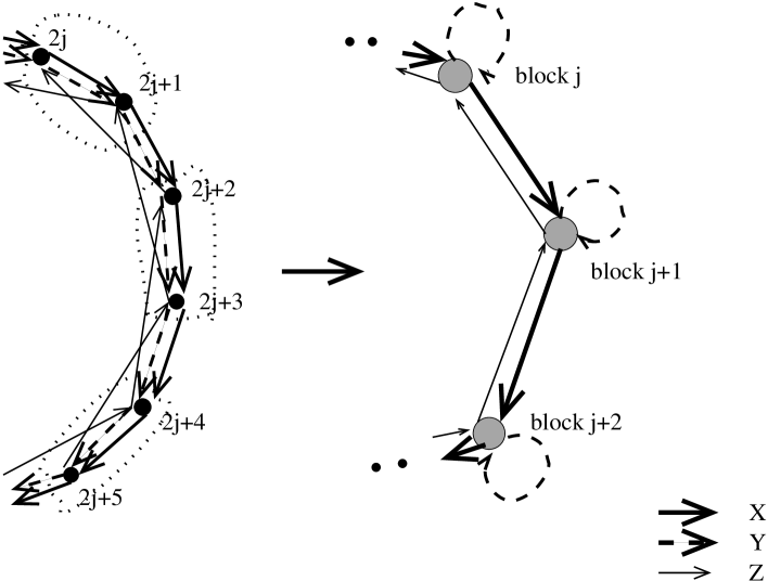
Figure 2: ${\mathbb{C}}^{3}/{\mathbb{Z}}_{N}(1,1,-2)\rightarrow{\mathbb{C}}^{2}/{\mathbb{Z}}_{N/2}(1,0,-1)$ : Coarse-graining as $(2j,2j+1)\rightarrow j$ by condensing the $X_{2j,2j+1}$ link. The $Y_{2j,2j+1}$ links become light neutral fields while $X_{2j-1,2j}$ and $Z_{j}^{+}={1\over 2}(Z_{2j,2j-2}+Z_{2j+1,2j-1})$ become light bifundamentals. This new quiver now represents ${\mathbb{C}}^{2}/{\mathbb{Z}}_{N/2}$. We have not shown the $Y_{2j-1,2j}$ and $Z_{j}^{-}$ links that become massive under the Higgsing.

The cubic part of the superpotential can be rewritten as

$${}W_{3}=\sum_{j=1}^{M}X_{2j+1}[Y_{2j+2}Z_{j+a+1}^{+}-Y_{2j-2a}Z_{j+1}^{+}]=\sum_{j=1}^{M}Z_{j}^{+}(X_{2j-2a-1}Y_{2j-2a}-X_{2j-1}Y_{2j-2a-2})$$

$${}\qquad\equiv\sum_{j=1}^{M}Z_{j,j-a-1}(X_{j-a-1,j-a}Y_{j-a,j}-X_{j-1,j}Y_{j-a-1,j-1})$$ (20)

In the last line, we have as before relabelled $(2j,2j+1)\rightarrow j$, so that this now looks like an ${\cal N}{=}1$ superpotential for the light fields $X_{2j+1},Z_{j}^{+},Y_{2j}$ relabelled as $X_{j,j+1},Z_{j,j-a-1},Y_{j,j+a},\ j=1,\ldots,{M}$. This is succinctly expressed diagrammatically as shown in some specific examples in figure 2, figure 3 and figure 4. More generally, looking at the quiver for $(1,2a+1,-2a-2)$, it is clear that, e.g. the light link $Y_{2j,2j+2a+1}$ connects the $j$-th and $(j+a)$-th blocks, so that the new quiver is $(1,a,-a-1)$. Thus the residual quiver represents a ${\mathbb{C}}^{3}/{\mathbb{Z}}_{M}$ geometry with the orbifold action $(1,a,-a-1)$ on the coordinates $X,Z^{+},Y$.

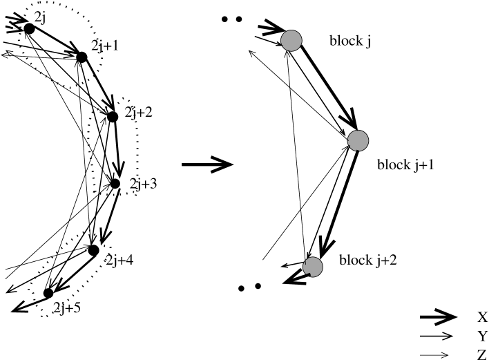
Figure 3: ${\mathbb{C}}^{3}/{\mathbb{Z}}_{N}:(1,2,-3)\rightarrow(1,1,-2)$ : Coarse-graining as $(2j,2j+1)\rightarrow j$ by condensing the $X_{2j,2j+1}$ link. Two of the four effective links between, e.g. blocks $j$ and $j+1$ become massive – these represent $Y_{j}^{-},Z_{2j+3,2j}$. Retaining only the light link fields gives the quiver on the right, i.e. $(1,1,-2)$.

3.2 Sequential Higgsing : $(1,2a,-2a-1)\rightarrow(1,a,-a-1)$

This subsection, very similar to the previous one, specializes to the case $(1,2a,-2a-1)$. Consider the D-term configuration $D_{i}=(-1)^{i}\rho$. The maximally symmetric vacua are then represented by

$$X_{2j}=\sqrt{\rho},\qquad j=1,\ldots,M={N\over 2}$$ (21)

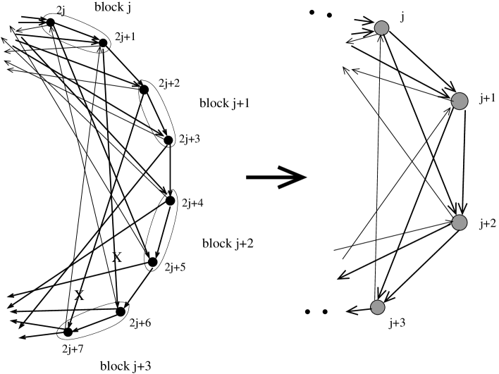
Figure 4: Example $a=2$ : ${\mathbb{C}}^{3}/{\mathbb{Z}}_{N}:(1,5,-6)\rightarrow(1,2,-3)$ : The links in the $(1,5,-6)$ quiver are $X_{i,i+1},Y_{i,i+5},Z_{i+6,i}$ and their conjugates. The process of coarse-graining as $(2j,2j+1)\rightarrow j$ by condensing the $X_{2j,2j+1}$ link gives masses to the links with an X marked on them as well as the linear combinations $Z^{+}$. Retaining only the light links gives the quiver on the right, i.e. $(1,2,-3)$.

as the only nonzero expectation values. This Higgses the $U(1)\times U(1)$ in each block down to the diagonal $U(1)$ as before. The superpotential is

$$W=W_{2}+W_{3},$$

$${}W_{2}=\sum_{j=1}^{M}X_{2j}(Y_{2j+1}Z_{2j+2a+1}-Y_{2j-2a}Z_{2j+1})$$

$${}\qquad=\sqrt{\rho}\sum_{j}Z_{2j+1}(Y_{2j-2a+1}-Y_{2j-2a})=\sqrt{\rho}\sum_{j}Z_{2j+2a+1}Y_{j}^{-},$$

$${}W_{3}=\sum_{j=1}^{M}X_{2j+1}(Y_{2j+2}Z_{2j+2a+2}-Y_{2j-2a+1}Z_{2j+2})$$ (22)

where we have defined $Y_{j}^{\pm}={1\over 2}(Y_{2j+1}\pm Y_{2j})$. Then the $Z_{2j+1}$ and $Y_{j}^{-}$ fields appearing in $W_{2}$ become massive. The classical equations of motion for $Z_{2j+1}$ following from $W$ give $Y_{j}^{-}=0$ so that

$$Y_{j}^{+}={1\over 2}(Y_{2j}+Y_{2j+1})=Y_{2j}=Y_{2j+1}$$ (23)

Then the cubic part of the superpotential can be rewritten as

$${}W_{3}=\sum_{j=1}^{M}X_{2j+1}[Z_{2j+2a+2}Y_{j+1}^{+}-Z_{2j+2}Y_{j-a}^{+}]=\sum_{j=1}^{M}Y_{j}^{+}(X_{2j-1}Z_{2j+2a}-X_{2j+2a+1}Z_{2j+2a+2})$$

$${}\qquad\equiv\sum_{j=1}^{M}Y_{j,j+a}(X_{j-1,j}Z_{j+a,j-1}-X_{j+a,j+a+1}Z_{j+a+1,j})$$ (24)

In the last line, we have as before relabelled $(2j,2j+1)\rightarrow j$, so that this now looks like an ${\cal N}{=}1$ superpotential for the light fields $X_{2j+1},Y_{j}^{+},Z_{2j}$ relabelled as $X_{j,j+1},Z_{j,j-a-1},Y_{j,j+a},\ j=1,\ldots,{N\over 2}$. The light link $Y_{j}^{+}$ in this case connects blocks $(j)$ and $(j+a)$ so that this again gives a $(1,a,-a-1)$ quiver. The residual quiver represents a ${\mathbb{C}}^{3}/{\mathbb{Z}}_{M}$ geometry with the orbifold action $(1,a,-a-1)$ on the coordinates $X,Y^{+},Z$. Figure 2 shows how the ${\mathbb{C}}^{3}/{\mathbb{Z}}_{2M}\ (1,1,-2)$ quiver flows to the ${\mathbb{C}}^{2}/{\mathbb{Z}}_{M}$ quiver. Similarly the ${\mathbb{C}}^{3}/{\mathbb{Z}}_{2M}\ (1,2,-3)$ quiver flows to ${\mathbb{C}}^{3}/{\mathbb{Z}}_{M}\ (1,1,-2)$ (figure 3). Figure 4 shows a slightly more complicated flow pattern. Thus in general, we think of the quiver as a lattice with $l$-th nearest neighbour interactions following from the orbifold projection. Then under the Higgsing, we flow progressively towards quivers with more local interactions.

4 Coarse-graining the “upstairs” matrices

In this section, we lift the Higgsing calculations described thus far to the “upstairs” $N\times N$ matrices of the image branes, thereby making connections to the matrix coarse-graining studied in [4]. To this end, consider the scalars $X,Y,Z$ of the parent ${\cal N}{=}4$ $U(N)$ theory after projection to the ${\mathbb{C}}^{2}/{\mathbb{Z}}_{N}$ orbifold, written as $N\times N$ matrices

$${}X=\left(\begin{array}[]{cccccc}0&X_{N1}&0&&&\\ &0&X_{12}&0&&\\ &&0&X_{23}&&\ldots\\ &&&0&&\\ &&&.&&\\ &&&.&&\\ \end{array}\right),\qquad Y=\left(\begin{array}[]{cccccc}0&&&&&Y_{N,N-1}\\ Y_{1N}&0&&&&\\ 0&Y_{21}&0&&&\\ &0&Y_{32}&\ldots&&\\ &&.&&&\\ &&.&&&\\ \end{array}\right),$$ (37)

$${}\qquad\qquad Z={\rm diag}[Z_{NN},Z_{11},Z_{22},\ldots,Z_{N-1,N-1}]$$ (38)

The orbifold projection ensures that these one-off-the-diagonal matrix elements are the only nonzero elements in these matrices. Further the projection also ensures that the gauge group is only the $U(1)^{N}$ subgroup of the full $U(N)$ in the parent theory so that the notion of nearest neighbour is physically well-defined in these matrix representations. These matrices do not commute for generic points on the orbifold moduli space, i.e. generic link field expectation values. It is important to note that the status of these matrices for the image branes is different from those in [4], since most of the entries do not exist here, due to the orbifold projection. We are simply using these “upstairs” matrices as a convenient device making contact with the ideas and calculations of [4].

In Higgsing the $U(1)_{2j}\times U(1)_{2j+1}\rightarrow U(1)$ in each pair (or block) by condensing the links $X_{2j,2j+1}$, we see that we have effectively bound the image branes as $(2j,2j+1)\rightarrow j$ at lower energies, thereby constructing a “block-brane” (for want of a more apt word). The fields $Y_{2j+1,2j},Z_{j}^{-}$ become massive. In [4], subtracting off the diagonal modes after coarse-graining in the (gauge-fixed) algebra of, e.g. the noncommutative plane, was found to yield a self-similar algebra with a new reduced noncommutativity parameter. Performing this procedure here produces the ${N\over 2}\times{N\over 2}$ matrices

$${}{\tilde{X}}=\left(\begin{array}[]{ccccccc}0&X_{12}&0&&&&\\ &0&X_{34}&0&&&\\ &&0&X_{56}&\ldots&&\\ &&&.&&&\\ &&&.&&&\\ \end{array}\right),\qquad{\tilde{Y}}=\left(\begin{array}[]{ccccccc}0&&&&&&Y_{N,N-1}\\ Y_{21}&0&&&&&\\ 0&Y_{43}&0&&&&\\ &0&Y_{65}&0&\ldots&&\\ &&&.&&&\\ &&&.&&&\\ \end{array}\right),$$ (50)

$${}\qquad\qquad{\tilde{Z}}={\rm diag}[{Z_{NN}+Z_{11}\over 2},{Z_{22}+Z_{33}\over 2}.\ldots]$$ (51)

Note that the diagonal modes we have removed correspond precisely to the fields $X_{2j,2j+1}$, $Y_{2j+1,2j},Z_{j}^{-}$, which have been eaten or given a mass by the Higgs mechanism. This is now the matrix representation of the scalars on the partially resolved ${\mathbb{C}}^{2}/{\mathbb{Z}}_{N/2}$ orbifold that the “block-brane” lives on. This is an interesting observation – coarse-graining [4] of the scalar matrices (with appropriate matrix-dependent averaging constants) followed by subtracting the massive modes (which here are the diagonal elements for the $X,Y$ matrices and the relative position coordinate in the $Z$ matrices) is precisely equivalent to the Higgsing analysis that we have carried out in the previous sections. It is important to note that the averaging constants are in general different for the different scalar matrices : e.g. $\alpha_{X}=\alpha_{Y}=1,\alpha_{Z}={1\over 2}$ is the set of averaging constants for ${\mathbb{C}}^{2}/{\mathbb{Z}}_{N}$ above. This anisotropy is not unexpected since the geometric meanings of the $X,Y$ matrices as link fields and the $Z$ matrices as position coordinates are on different footings. Furthermore the conditions in eqn. (40) of [4] are precisely the same as the hierarchies on the Higgs expectation values for the $X_{i,i+1}$ with $\alpha_{X}=1$

$$\biggl{|}{{\tilde{X}}_{a,a+1}\over X_{a,a+1}}\biggr{|}=\biggl{|}{X_{2a,2a+1}\over X_{a,a+1}}\biggr{|}<1$$ (52)

except that these conditions on the expectation values now reflect the fact that the brane worldvolume gauge theory is sequentially being truncated to lower energies under the process of coarse-graining. It is amusing to note that these same equations represent conditions for reducing noncommutativity (as defined in [4]) from the point of view of the “upstairs” scalar matrices. Furthermore, it is now clear that requiring these conditions to be satisfied in the orbifold examples identifies precisely those regions of moduli space that exhibit the corresponding hierarchies of energy scales in the expectation values (or alternatively in the sizes of the closed string blowup modes in the geometry) ensuring that this block-spin-like transformation is Wilsonian on the worldvolume.

It is easy to realize the same analysis for the other geometries we have studied. For instance, consider the scalars $X,Y,Z$ of the parent ${\cal N}{=}4$ $U(N)$ theory after projection to the ${\mathbb{C}}^{3}/{\mathbb{Z}}_{N}$ orbifold with action $(1,1,-2)$, written as $N\times N$ matrices

$${}X=\left(\begin{array}[]{ccccccc}0&X_{N1}&0&&&&\\ &0&X_{12}&0&&&\\ &&0&X_{23}&0&&\\ &&&0&X_{34}&\ldots&\\ &&&.&&&\\ &&&.&&&\\ \end{array}\right),\qquad Y=\left(\begin{array}[]{ccccccc}0&Y_{N1}&0&&&&\\ &0&Y_{12}&0&&&\\ &&0&Y_{23}&0&&\\ &&&0&Y_{34}&\ldots&\\ &&&.&&&\\ &&&.&&&\\ \end{array}\right),$$ (65)

$${}\qquad\qquad Z=\left(\begin{array}[]{ccccccc}0&&&&\ldots&Z_{N,N-2}&0\\ 0&0&&&\ldots&0&Z_{1,N-1}\\ Z_{2N}&0&0&&&&\\ 0&Z_{31}&0&&&&\\ &0&Z_{42}&&\ldots&&\\ &&&.&&&\\ &&&.&&&\\ \end{array}\right)$$ (73)

As before, we coarse-grained the quiver as $(2j,2j+1)\rightarrow j$, by condensing the links $X_{2j,2j+1}$ (these get eaten). Here it is the fields $Y_{2j-1,2j},Z_{j}^{-}$ that become massive. Then the above matrices coarse-grain as

$${\tilde{X}}=\left(\begin{array}[]{ccccccc}0&X_{12}&0&&&&\\ &0&X_{34}&0&&&\\ &&0&X_{56}&&\ldots&\\ &&&.&&&\\ &&&.&&&\\ \end{array}\right),\qquad{\tilde{Y}}=\left(\begin{array}[]{ccccccc}Y_{1N}&0&&&&&\\ 0&Y_{23}&0&&&&\\ &0&Y_{45}&0&\ldots&&\\ &&&.&&&\\ &&&.&&&\\ \end{array}\right),$$ (84)

$${\tilde{Z}}=\left(\begin{array}[]{ccccccc}0&&&&\ldots&Z_{N,N-2}+Z_{1,N-1}&\\ Z_{2N}+Z_{31}&0&&&&&\\ 0&Z_{42}+Z_{53}&0&&&&\\ &&&.&&&\\ &&&.&&&\\ \end{array}\right)$$ (90)

where we have retained only the light fields as before. Note that the scalar $Y$ has only diagonal elements now, so that it is a neutral field now. This is the matrix representation of the scalars on the partially resolved ${\mathbb{C}}^{2}/{\mathbb{Z}}_{N/2}$ orbifold with coordinates $X,Z^{+}$ that the “block-brane” lives on.
Consider now the scalars $X,Y,Z$ of the parent ${\cal N}{=}4$ $U(N)$ theory after projection to the ${\mathbb{C}}^{3}/{\mathbb{Z}}_{N}$ orbifold with action $(1,2,-3)$, written as $N\times N$ matrices

$${}X=\left(\begin{array}[]{ccccccc}0&X_{N1}&0&&&&\\ &0&X_{12}&0&&&\\ &&0&X_{23}&0&&\\ &&&0&X_{34}&\ldots&\\ &&&.&&&\\ &&&.&&&\\ \end{array}\right),\qquad Y=\left(\begin{array}[]{ccccccc}0&0&Y_{N2}&0&&\\ &0&0&Y_{13}&0&\\ &&0&0&Y_{24}&0&\\ &&&0&0&Y_{35}&\ldots\\ &&&.&&&\\ &&&.&&&\\ \end{array}\right),$$ (103)

$${}\qquad\qquad Z=\left(\begin{array}[]{ccccccc}0&&&\ldots&Z_{N,N-3}&0&0\\ 0&&&\ldots&0&Z_{1,N-2}&0\\ 0&0&&\ldots&&0&Z_{2,N-1}\\ Z_{3N}&0&0&&&&\\ 0&Z_{41}&0&\ldots&&&\\ &&&.&&&\\ &&&.&&&\\ \end{array}\right)$$ (111)

We coarse-grained the quiver as $(2j,2j+1)\rightarrow j$, by condensing the links $X_{2j,2j+1}$ (these get eaten). The fields $Z_{2j+3,2j},Y_{j}^{-}$ become massive. Then the above matrices coarse-grain as

$${}{\tilde{X}}=\left(\begin{array}[]{ccccccc}0&X_{12}&0&&&&\\ &0&X_{34}&0&&&\\ &&0&X_{56}&\ldots&\\ &&&.&&&\\ &&&.&&&\\ \end{array}\right),\qquad{\tilde{Y}}=\left(\begin{array}[]{ccccccc}0&Y_{N2}+Y_{13}&0&&&&\\ &0&Y_{24}+Y_{35}&0&\ldots&&\\ &&&.&&&\\ &&&.&&&\\ \end{array}\right),$$ (121)

$${}{\tilde{Z}}=\left(\begin{array}[]{ccccccc}0&&&&\ldots&Z_{N,N-3}&0\\ 0&0&&&\ldots&0&Z_{2,N-1}\\ Z_{41}&0&0&&\ldots&&\\ &&&&.&&\\ &&&&.&&\\ \end{array}\right)$$ (127)

where we have retained only the light fields. It is clear that this is the matrix representation of the scalars on the partially resolved ${\mathbb{C}}^{3}/{\mathbb{Z}}_{N/2}$ orbifold with action $(1,1,-2)$ on coordinates $X,Y^{+},Z$ that the “block-brane” lives on.
It is not too hard to show that the matrix representations of the more general ${\mathbb{C}}^{3}/{\mathbb{Z}}_{N}$ quivers that we considered exhibit similar properties. Note that in [4], subtracting off the diagonal modes after coarse-graining in the (gauge-fixed) algebra of, e.g. the noncommutative plane was found to yield a self-similar algebra with a new reduced noncommutativity parameter – however it was not clear if this was a prescription compatible with Wilsonian renormalization organized by the energy scales involved. We see now from the orbifold examples here that we can identify matrix coarse-graining as defined in [4] as a Wilsonian process if we first coarse-grain the matrices and then subtract off precisely the modes that are massive under the Higgs expectation values that we have given. It would be interesting to analyze more general D-brane configurations along these lines, incorporating the more serious issues of gauge invariance present in general.

It is an interesting question to generalize this equivalence between this matrix coarse-graining, these block-spin-like transformations and field theoretic renormalization to more general scenarios with real D-branes and fluxes, with a view to understanding the flows in geometries that this generates.

5 The structure of flows in the space of quivers

To recap, in the region of moduli space in which we carried out our calculations, the sequence of Higgs transitions represents a sequence of partial blowups of the quotient singularity. In the sense discussed above in detail, it corresponds to block-spin-like transformations on the image branes. Thinking of the quiver as a lattice these were analogous to coarse-graining transformations. Furthermore, lifting this process to the “upstairs” matrices makes contact with the matrix coarse-graining of [4]. This process can be represented diagrammatically as we have seen in the figures. In this section, we will map out the structure of the flows we have obtained.

Under a $(2\times 2)$-block coarse-graining, we have seen that, e.g. a ${\mathbb{C}}^{3}/{\mathbb{Z}}_{N}\ (1,2a,-2a-1)$ quiver flows to a ${\mathbb{C}}^{3}/{\mathbb{Z}}_{N/2}\ (1,a,-a-1)$ quiver. Continuing the process we see from the change in $a$ that the quiver is becoming progressively “more local.” Eventually, the process leads to a ${\mathbb{C}}^{2}/{\mathbb{Z}}_{N^{\prime}}$ quiver. In our spin system analogy, this type of quiver corresponds to a local interaction (with range small compared to the correlation length of the system). By contrast, if we consider the quotient with $a$ of order $N$, which corresponds to a highly nonlocal interaction, our successive coarse-graining transformations produce a sequence of quivers with comparable measures of “non-locality.” Further, while we have not shown this explicitly, it is not too hard to see from the quiver diagrams that changing block size to, say $l\times l$ blocks, does not change the qualitative structure of the coarse-graining we have shown for these quivers.

Consider now the space of quiver models, restricting attention to lowest order in $\alpha^{\prime}$ and $g_{s}$, with no background fluxes. A point in this subset can be described as ${\mathbb{C}}^{3}/{\mathbb{Z}}_{N}$ with orbifold action $(1,a_{2},a_{3})$. This simplified subset of the space of quiver models is thus a lattice-like space: a point in this space is labelled by $(N,a_{2},a_{3})$. Restricting attention to supersymmetric vacua is equivalent to restricting to the subspace with $\ 1+a_{2}+a_{3}=0$. Under these block-spin-like transformations, we have seen that ${\mathbb{C}}^{3}/{\mathbb{Z}}_{N}$ for finite $N$ flows to the point $(0,0,0)$: this is flat space and it is a fixed point. The number of iterations required is $O(\log N)$. Thus as $N$ grows large, the number of iterations diverges and an RG-like approach is valid. We have also seen that the ${\mathbb{C}}^{2}/{\mathbb{Z}}_{N}$ quiver for any $N$ flows towards flat space. Furthermore, the ${\mathbb{C}}^{3}/{\mathbb{Z}}_{N},\ a_{i}\ll N$, quivers flow towards ${\mathbb{C}}^{2}/{\mathbb{Z}}_{N}$ quivers, before finally flowing to flat space, enhancing supersymmetry from ${\cal N}{=}1$ to ${\cal N}{=}2$ to finally ${\cal N}{=}4$. Figure 5 summarizes the flows in quiver space.

Figure 5: The structure of flows : The general point in this simplified subset of the space of quivers is ${\mathbb{C}}^{3}/{\mathbb{Z}}_{N},\ (1,a,-a-1)$, which we have labelled in this $(N,a)$-plane. Flat space with ${\cal N}{=}4$ supersymmetry is a fixed point. All flowlines end finally at flat space. However the ${\mathbb{C}}^{3}/{\mathbb{Z}}_{N},\ a\ll N$ quivers flow towards ${\mathbb{C}}^{2}/{\mathbb{Z}}_{N}$ quivers before flowing finally to flat space, enhancing supersymmetry from ${\cal N}{=}1$ to ${\cal N}{=}2$ to finally ${\cal N}{=}4$.

It is worthwhile to note that these theories that we have been considering are each good supersymmetric D-brane configurations (or string vacua) in themselves. Thus this block-spin-like transformation we have described here is really a flow in the (simplified subset of the) space of D-brane configurations.

Now it is clear that if the brane sits $at$ the orbifold singularity, all the link modes are massless and there is no hierarchy of scales. However in the region of moduli space where the link expectation values exhibit a wide hierarchy of scales, this transformation exhibits an interesting structure of flows and fixed points that are self-similar. Note though that this region of moduli space is not unique : e.g. for ${\mathbb{C}}^{2}/{\mathbb{Z}}_{N}$ via $(2\times 2$ blocks, we condensed links $X_{2j,2j+1}$, which is Wilsonian in the region with the hierarchies $|X_{12}|<|X_{N1}|$ and so on, while condensing the $X_{2j-1,2j}$ links gives a different region of moduli space. However while the regions in moduli space are different, the qualitative features of the flows – the directions of the flows and the fixed points – are the same.

The description above is of course a highly simplified picture of the space of quiver gauge theories appearing on the worldvolumes of D-branes probing orbifolds. Considering more general theories (e.g., ${\mathbb{R}}^{6}/\Gamma$, where $\Gamma$ is some discrete group, possibly with additional background fluxes turned on) imparts further structure to this space of quivers. It would be interesting to understand if this or any other kind of RG-like transformation can be constructed in more generality, possibly relating it to the ideas of [14].

6 Conclusions

We have described a block-spin-like transformation that coarse-grains quivers by sequentially Higgsing the gauge symmetry in these theories and exhibited the pattern of flows obtained thereby. Since the points in the space of quivers that we have discussed above are distinct string vacua, this transformation generates flows in this simplified subset of the space of D-brane configurations (or string vacua). In hindsight, the general schematic picture of matrix coarse-graining described in [4] would heuristically be expected to generate flows in the space of D-brane configurations, modulo the gauge-fixing problems there. It is thus an interesting open question to extend this block-spin-type procedure we have described here to more general D-brane configurations. Unlike the quiver examples here, understanding the analog of “nearest neighbour” is more subtle in general, e.g. where the gauge group is $U(N)$. We expect that this question is closely intertwined with issues of locality in both real space and its reflection in the space of matrices, as noted in the gauge-fixing problems observed in [4]. Understanding how to incorporate locality in a gauge-invariant fashion might in turn be related to hierarchies in the strengths of the link expectation values, something that has been relatively easy to nail down in the quiver examples here. It is interesting to ask if there is any notion of universality in the flows that would be generated in the space of geometries for general D-brane configurations, or more generally string vacua.

As we have seen in section 4, our description of the quiver flows makes contact with the matrix coarse-graining of [4] when the Higgsing process is lifted to the “upstairs” $N\times N$ matrices of the $N$ image branes for a $Z_{N}$ quotient singularity. These “upstairs” matrices are noncommuting for generic expectation values of the bifundamental fields “downstairs” (i.e. generic points in the orbifold moduli space). Then, as have seen in section 4, the conditions for reducing noncommutativity (as defined in [4]) of the “upstairs” matrices coincide with the conditions on the region of moduli space for the process to be Wilsonian on the worldvolume “downstairs”. Thus the orbifold computations described here provide a concrete field theoretic realization of the matrix coarse-graining of [4]. Furthermore, since the gauge group after orbifold projection is $U(1)^{N}$, the gauge invariance problems of the matrix RG of [4] are absent here.

For the quiver theories, this process defines a kind of deconstructive RG in theory space with the corresponding RG flows as described in the previous section. This is a kind of real space RG that coarse-grains the extra dimension. From this point of view, we find that the large $N$ limit of ${\mathbb{C}}^{2}/{\mathbb{Z}}_{N}$ (in this region of orbifold moduli space) appears to deconstruct an inhomogeneous continuum extra dimension. Such an extra dimension is fractal in the sense that there is self-similarity at arbitrarily short distances. Note that this process is different from applying conventional blockspin-type techniques on the lattice gauge theory in the extra dimension. A uniform extra dimension, generated by equal expectation values for the link fields, does not exhibit any hierarchy of energy scales and so an RG by sequentially integrating out massive link expectation values is not possible along the lines we have studied here. Presumably conventional blockspin-type techniques (or momentum space RG in the extra dimensions) could be applied to study such an RG at a field theoretic level.

Finally, it is important to note that this scheme of coarse-graining via condensing link expectation values in these supersymmetric theories turns on marginal deformations from the point of view of the corresponding worldsheet string theory in this background. A natural question is what the corresponding story is for nonsupersymmetric orbifolds with localized closed string tachyons [17] [18]. These orbifolds typically have both relevant (tachyonic) and marginal closed string twisted sector modes. Assuming that the system does not run away along the directions with tachyonic instabilities, we can extend the above analysis to the marginal modes. On the other hand, turning on a tachyonic (relevant) deformation on the worldsheet corresponds to evolution in time in the target space, i.e. the worldsheet RG scale corresponds to time in the target space. It is interesting to ask what the relation of this block-spin-like transformation is, if any, to these tachyonic flows.

Acknowledgments: It is a pleasure to thank P. Argyres, P. Aspinwall, M. Douglas, P. Horava, S. Kachru, I. Melnikov, D. Morrison, M. Rangamani, S. Rinke, A. Sen, S. Trivedi, M. van Raamsdonk and H. Verlinde for helpful discussions. KN thanks the organizers of the HRI String workshop, Allahabad, India, for hospitality during incipient stages of this work, as well as hospitality of the Theory Group at UC Berkeley during stages of this work. MRP thanks KITP and the organisers of the Geometry, Topology, and Strings workshop (MP03) where some of this work was completed. His participation was supported in part by the National Science Foundation under Grant No. PHY99-07949. This work is partially supported by NSF grant DMS-0074072.

Appendix A Interpolating expectation values

In this appendix, we construct a set of Higgs expectation values which interpolate between the equal expectation values limit $h\neq 0,\rho_{i}\sim 0$ and our hierarchical limit $h\sim 0,\rho_{i}\neq 0$. Let us do this sequentially so as to break the $Z_{N}$ discrete symmetry but retain a $Z_{N/2}$ subgroup thereof. If we restrict attention to real expectation values for $X_{i},Y_{i}$ with $Z_{i}=0$, it is sufficient, instead of (3) and (4), to solve

$$X_{2j}^{2}Y_{2j}^{2}=X_{2j-1}^{2}Y_{2j-1}^{2}=X_{2j-2}^{2}Y_{2j-2}^{2},$$

$$|X_{2j}|^{2}-|Y_{2j}|^{2}-|X_{2j-1}|^{2}+|Y_{2j-1}|^{2}=\rho_{2j} = \rho,$$

$$|X_{2j-1}|^{2}-|Y_{2j-1}|^{2}-|X_{2j-2}|^{2}+|Y_{2j-2}|^{2}=\rho_{2j-1} = -\rho$$ (128)

to execute sequential Higgsing. It is clear that a solution that preserves the $Z_{N/2}$ subgroup can be found by redefining

$$a_{2j-1}=X_{2j-1}^{2}=a_{1},\ b_{2j-1}=Y_{2j-1}^{2}=b_{1},\ \ \ a_{2j}=X_{2j}^{2}=a_{2},\ a_{2j}=Y_{2j}^{2}=b_{2},\qquad j=1,\ldots{N\over 2}$$ (129)

to find a solution to this $2\times 2$ block within the $Z_{N}$ and then repeat it $N/2$ times preserving $Z_{N/2}$. Thus it is sufficient to find solutions to

$$a_{2}b_{2}=a_{1}b_{1},\qquad a_{2}-a_{1}-b_{2}+b_{1}=\rho$$ (130)

such that for ${\rho\over h}\ll 1$, we have the probe on the unresolved orbifold with $a_{2}=a_{1}=b_{1}=b_{2}=h$, while ${\rho\over h}\gg 1$ yields the partially resolved limit with $a_{2}=\rho,a_{1}=b_{1}=b_{2}=0$. It is not too hard to show that

$$x=1-\tanh{\rho\over h},\qquad\qquad X_{2j-1}^{2}=a_{1}=hx, {}\qquad X_{2j}^{2}=a_{2}=h\biggl{(}{{\rho\over h}+x+x^{2}\over 1+x}\biggr{)},$$

$$Y_{2j-1}^{2}=b_{1}=hx\biggl{(}{{\rho\over h}+x+x^{2}\over 1+x}\biggr{)}, {}\qquad Y_{2j}^{2}=b_{2}=hx^{2}$$ (131)

is a set of solutions to the F- and D-term equations that does the interpolation. This gives rise to a hierarchy of scales where the $X_{2j}$ expectation values become more massive than the rest as we increase $\rho$.

References

- [1] T. Banks, W. Fischler, S. Shenker, L. Susskind, “M-theory as a Matrix model : a conjecture”, Phys. Rev. D55, 5112 (1997), [hep-th/9610043, on http://arxiv.org].
- [2] See, e.g., the review, O. Aharony, S. .Gubser, J. Maldacena, H. Ooguri, Y. Oz, “Large N field theories, string theory and gravity”, Phys. Rept. 323, 183 (2000), [hep-th/9905111].
-
[3]
Besides various textbooks, the following papers/reviews give a good
description of block spins, Kadanoff scaling and critical phenomena :
K. G. Wilson, “Renormalization group and critical phenomena 1 : renormalization group and the Kadanoff scaling picture”, Phys. Rev. B4 3174 (1971);
“Renormalization group and critical phenomena 2 : Phase space cell analysis of critical behaviour”, Phys. Rev. B4 3184 (1971);
“The renormalization group : critical phenomena and the Kondo problem”, Rev. Mod. Phys. 47 773 (1975);
“The renormalization group and block spins”, Cornell U. preprint CLNS-319, Oct 1975;
K. G. Wilson, J. Kogut, “The renormalization group and the -expansion”, Phys. Rep. 12 75 (1974);
S. Shenker, Les Houches 1982 lectures on field theory and phase transitions;
J. Kogut, “Introduction to lattice gauge theory and spin systems”, Rev. Mod. Phys. 51, 659 (1979). - [4] K. Narayan, “Blocking up D-branes : Matrix renormalization ?” [hep-th/0211110].
- [5] M. Douglas, G. Moore, “D-branes, quivers and ALE instantons”, [hep-th/9603167].
- [6] Y. Ito and M. Reid, “The McKay Correspondence for Finite Subgroups of ”, in M. Andreatta et al., editors, “Higher Dimensional Complex Varieties”, pages 221–240, de Gruyter, 1996, [alg-geom/9411010].
- [7] J. Polchinski, “Tensors from K3 orientifolds”, Phys. Rev. D55, 6423 (1997), [hep-th/9606165].
- [8] C. Johnson, R. Myers, Aspects of Type IIB theory on ALE spaces”, Phys. Rev. D55, 6382 (1997), [hep-th/9610140].
- [9] N. Arkani-Hamed, A. Cohen, H. Georgi, “(De)constructing dimensions”, Phys. Rev. Lett. 86, 4757 (2001), [hep-th/0104005]; C. Hill, S. Pokorski, J. Wang, “Gauge-invariant effective lagrangian for Kaluza-Klein modes”, Phys. Rev. D64, 105005 (2001), [hep-th/0104035].
- [10] For the deconstruction limit, see e.g. I. Rothstein, W. Skiba, “Mother Moose : generating extra dimensions from simple groups at large ”, Phys. Rev. D65, 065002 (2002), [hep-th/0109175], N. Arkani-Hamed, A. Cohen, D. Kaplan, A. Karch, L. Motl, “Deconstructing and little string theories”, JHEP 0301, 083 (2003), [hep-th/0110146]; A. Adams, M. Fabinger, “Deconstructing noncommutativity with a giant fuzzy moose”, JHEP 0204, 006 (2002), [hep-th/0111079].
- [11] M. Douglas, B. Greene, D. Morrison, “Orbifold resolution by D-branes”, Nucl. Phys. B506, 84 (1997), [hep-th/9704151].
- [12] D. Morrison, M. Ronen Plesser, “Nonspherical horizons”, Adv. Theor. Math. Phys. 3, 1 (1999), [hep-th/9810201].
- [13] L. Ibanez, R. Rabadan, A. Uranga, “Anomalous U(1)s in Type I and Type IIB , string vacua”, Nucl. Phys. B542, 112 (1999), [hep-th/9808139].
- [14] M. R. Douglas, “The statistics of string/M vacua”, [hep-th/0303194]; L. Susskind, “The anthropic landscape of string theory”, [hep-th/0302219].
- [15] C. Hill, “Fractal theory space : space-time of noninteger dimensionality”, Phys. Rev. D67, 085004 (2003), [hep-th/0210076] ; “Geometrical renormalization groups : perfect deconstruction actions”, [hep-th/0303267].
- [16] N. Arkani-Hamed, A. Cohen, H. Georgi, “Twisted supersymmetry and the topology of theory space”, JHEP, 0207, 020 (2002), [hep-th/0109082].
- [17] A. Adams, J. Polchinski, E. Silverstein, “Don’t panic ! Closed string tachyons in ALE spacetimes”, JHEP, 0110, 029 (2001), [hep-th/0108075].
- [18] J. Harvey, D. Kutasov, E. Martinec, G. Moore, “Localized tachyons and RG flows” [hep-th/0111154] ; see also, e.g., E. Martinec, “Defects, decay and dissipated states”, [hep-th/0210231].