GEF-TH-9-2003

Physical States at the Tachyonic Vacuum of Open
String Field Theory
S. Giusto and C. Imbimbo
Dipartimento di Fisica, Università di Genova
and
Istituto Nazionale di Fisica Nucleare, Sezione di Genova
via Dodecaneso 33, I-16146, Genoa, Italy

We illustrate a method for computing the number of physical states of open string theory at the stable tachyonic vacuum in level truncation approximation. The method is based on the analysis of the gauge-fixed open string field theory quadratic action that includes Fadeev-Popov ghost string fields. Computations up to level 9 in the scalar sector are consistent with Sen’s conjecture about the absence of physical open string states at the tachyonic vacuum. We also derive a long exact cohomology sequence that relates relative and absolute cohomologies of the BRS operator at the non-perturbative vacuum. We use this exact result in conjunction with our numerical findings to conclude that the higher ghost number non-perturbative BRS cohomologies are non-empty.

1 Introduction

With the advent of D-branes it has been understood that bosonic open strings are excitations of an unstable solitonic object of bosonic closed string theory. This lead Sen to conjecture [1, 2] that the non-linear classical equations of motion of open string field theory (OSFT) [3] possess a translation invariant solution whose energy density exactly cancels the brane tension. The existence of a solution with such a property has been persuasively demonstrated [5, 6, 7] within the level truncation (LT) expansion of OSFT [4]. This solution, where the tachyon open string field is condensed, is believed to be the stable non-perturbative vacuum of OSFT representing the closed string vacuum with no open strings.

The most basic expected property of OSFT around the tachyonic vacuum is the absence of solutions of the linearized equation of motions that are not pure gauge: this is what the conjecture that the stable vacuum has no open string excitations means. The kinetic operator of the OSFT action expanded around the non-perturbative vacuum solution is a nilpotent operator ${\widetilde{Q}}$ that acts on the first quantized open string state space: the linearized equations of motion around the tachyonic vacuum write in momentum space as

$${\widetilde{Q}}(p)\,\psi^{(0)}(p)=0$$ (1)

where $\psi^{(0)}(p)$ is an open string state of ghost number 0 and space-time momentum $p$. The space of solutions of the linearized equations of motion (1) modulo (linearized) gauge transformations is the cohomology of ${\widetilde{Q}}(p)$ on open string states of ghost number 0: it describes physical particles with mass squared $m^{2}=-p^{2}$. Thus, in short, Sen’s expectation is that the cohomology of ${\widetilde{Q}}$ at ghost number 0 — that we will denote by ${\cal H}^{\scriptscriptstyle(0)}({\widetilde{Q}})$ — vanishes for all $p^{2}$.

Computing the cohomology ${\cal H}^{\scriptscriptstyle(0)}({\widetilde{Q}})$ within the LT approximation scheme faces one basic difficulty: by restricting the state space to states of maximal level $L$ one breaks gauge invariance and replaces ${\widetilde{Q}}$ by a level truncated operator ${\widetilde{Q}}_{L}$ which is not nilpotent. Thus the image of ${\widetilde{Q}}_{L}$ does not lie in the kernel of ${\widetilde{Q}}_{L}$. The task therefore is to understand which solution of the level truncated linearized equations of motion should be considered gauge-trivial. The authors of [8] proposed to measure the triviality of a ${\widetilde{Q}}_{L}$-closed state by its orthogonal projection onto the image of ${\widetilde{Q}}_{L}$. This definition requires a positive definite hermitian product, with respect to which the orthogonal projection is defined. Although the open string state space is equipped with a unique ${\widetilde{Q}}$-invariant hermitian product, this is not positive definite — precisely because ${\widetilde{Q}}$ is nilpotent. For this reason the authors of [8] select an arbitrary positive definite hermitian product with respect to which “approximate” gauge-triviality of ${\widetilde{Q}}_{L}$-closed states is defined.

This way to compute ${\cal H}^{\scriptscriptstyle(0)}({\widetilde{Q}})$ may be subject to two kinds of criticism. First, the choice of a positive definite hermitian product is arbitrary and it is not clear, a priori, why it should be irrelevant. The authors of [8] did verify that by taking two different positive definite hermitian products their definition of “approximate” gauge-triviality does not change much, but there is no theoretical reason why this should be so in general: if a vector does not belong in a given subspace of a vector space, it is always possible to define a definite positive hermitian product with respect to which the vector and the subspace are orthogonal.

Second, any method that computes ${\widetilde{Q}}$ cohomology by looking at the kernel of the level truncated ${\widetilde{Q}}_{L}$ can only detect a certain type of cohomology. To understand this, let us remark that the linear equations (1) have two kinds of solutions: the $\psi^{(0)}(p)$’s that are solutions for $p$ generic and those that are solutions for isolated values of $p$. We will call the former solutions of type A and the latter solutions of type B. As we will review in Section 5, type B solutions are not gauge-trivial, while type A solutions are gauge-trivial for $p$ generic, but they may become non-trivial at isolated values of $p$. Type B solutions are stable in the LT approximation: they can be deformed but they are not expected to disappear if the level is sufficiently big. Type A solutions instead are lifted by the LT approximation for generic values of $p$ since ${\widetilde{Q}}_{L}$ is not nilpotent: generically, the values of $p^{2}$ at which a type A solution survives in the LT theory do not coincide with the values of $p^{2}$ at which the solution of the exact theory may be non-trivial. In summary, if one only looks at the solutions of the level truncated version of the linearized equations of motion (1), one misses cohomology of type A, if this happens to exist.

We will explain in Section 5 that ${\widetilde{Q}}$-cohomology of type A at ghost number $n$ is in one-to-one correspondence with cohomology of type B at ghost number $n-1$. For example, the perturbative linearized equations of motion (which are the same as Eqs. (1) with ${\widetilde{Q}}$ replaced by the BRS charge $Q$ of the 2-dimensional CFT background) only have non-trivial solutions of type B, since the perturbative BRS cohomology at ghost number -1 is empty (at non-exceptional momenta): we do not know of any reason to assume that this holds also for the non-perturbative ${\widetilde{Q}}$.

For these reasons, we develop in this paper a method to compute ${\cal H}^{\scriptscriptstyle(0)}({\widetilde{Q}})$ in the LT approximation which starts from the gauge-fixed OSFT action around the tachyonic vacuum, that we present in Section 2. In Siegel gauge, the gauge-fixed kinetic operator for the matter string field is the operator

$${\widetilde{L}}_{0}\equiv\{{\widetilde{Q}},b_{0}\}$$ (2)

acting on states of ghost number 0. The gauge-fixed OSFT action includes also an infinite series of second quantized ghost fields, whose kinetic operators are again given by the operator in (2) acting on states of non-vanishing ghost number $n$. The gauge-fixed kinetic operators for both matter and ghost string fields acting on states of momentum $p$ will be denoted by ${\widetilde{L}}_{0}^{\scriptscriptstyle(n)}(p)$, with $n=0,1,\ldots$. The assumption that Siegel gauge is a good gauge for the theory around the non-perturbative vacuum [7] means that the kinetic operators ${\widetilde{L}}_{0}^{\scriptscriptstyle(n)}(p)$ do not have zero modes for generic values of $p^{2}$. ${\widetilde{L}}_{0}^{\scriptscriptstyle(n)}(p)$ may have zero modes at isolated values of $p^{2}=-m^{2}$ and these zeros are connected with physical states of mass $m$. In a theory without gauge invariance, if the determinant $\det{\widetilde{L}}_{0}^{\scriptscriptstyle(0)}(p)$ has a zero of order $d$ for $p^{2}=-m^{2}$ there are $d$ physical degrees of freedom of mass $m$. In a gauge theory, ghost fields contribute to the physical degrees of freedom counting: if $\det{\widetilde{L}}_{0}^{\scriptscriptstyle(n)}(p)$ has a zero of order $d_{n}$ for $p^{2}=-m^{2}$, the number of physical degrees of freedom of mass $m$ — which in OSFT is the dimension of ${\cal H}^{\scriptscriptstyle(0)}({\widetilde{Q}})|_{p^{2}=-m^{2}}$ — is given by the Fadeev-Popov index:

$$I_{FP}(m)=d_{0}-2\,d_{1}+2\,d_{2}+\cdots=\sum_{n=-\infty}^{\infty}(-1)^{n}\,d_{n}$$ (3)

Our method to compute the dimension of ${\cal H}^{\scriptscriptstyle(0)}({\widetilde{Q}})$ in LT approximation consists in counting the zeros of the determinants of the level truncated kinetic operators $({\widetilde{L}}_{0}^{\scriptscriptstyle(n)})_{L}(p)$. Of course degenerate zeros of $\det{\widetilde{L}}_{0}^{\scriptscriptstyle(n)}(p)$ of the exact theory will correspond to zeros of the level truncated $\det({\widetilde{L}}_{0}^{\scriptscriptstyle(n)})_{L}(p)$ that are only approximately degenerate. If the level is sufficiently big, we expect that zeros of $\det({\widetilde{L}}_{0}^{\scriptscriptstyle(n)})_{L}(p)$ group into approximately degenerate multiplets well separated among each other: in the level truncated theory, the index $I_{FP}$ in (43) should therefore be computed by including the zeros which belong to the same approximate multiplet. Sen’s conjecture is that Fadeev-Popov index for every multiplet vanishes. In order for this computation to make sense the level has to be big enough that the splitting among zeros belonging to the same multiplet is significantly smaller than the separation between multiplets.

In Section 3 we describe the results of our numerical study of the operators ${\widetilde{L}}_{0}^{\scriptscriptstyle(n)}$: we restricted ourselves to the Lorentz scalar states to limit the numerical complexity of the computation, although the extension of our method to higher spin states is in principle straightforward and physically more interesting. We found that, for levels from 4 to 9, the LT evaluation of the FP index $I_{FP}$ seems legitimate in the region $p^{2}\gtrsim-5$: in this range of $p^{2}$ we found a single approximate multiplet at $p^{2}=-{\bar{m}}^{2}\approx-2.1$. The Fadeev-Popov index of this multiplet vanishes and we verified that its spreading decreases as the level goes up.

Since the zeros of the gauge-fixed kinetic operators ${\widetilde{L}}_{0}^{\scriptscriptstyle(n)}(p)$ of the exact theory are isolated, we expect them to be more stable in LT than the zeros of the kinetic operator ${\widetilde{Q}}(p)$ of the gauge-invariant OSFT action. This is, in our view, the main advantage of our method with respect to previous ones. We expect that in a fixed region of $p^{2}$, once the level is high enough, no new zeros of the determinants $\det{\widetilde{L}}_{0}^{\scriptscriptstyle(n)}(p)$ will flow in from infinity as the level increases. On the other hand, it might happen that, for intermediate values of the level, pairs of zeros of the level truncated $\det({\widetilde{L}}_{0}^{\scriptscriptstyle(n)})_{L}(p)$ disappear and reappear. We found that for $p^{2}\approx-6$ there is indeed another multiplet of zeros whose index vanishes for levels 5 and 6 and becomes 4 for levels 7,8,9, due to the disappearance of a pair of zeros of $\det{\widetilde{L}}_{0}^{\scriptscriptstyle(-1)}$: it is not inconceivable that at levels higher than 9 this pair of zeros reappears.

Our computation determined the quadratic part of the gauge-fixed OSFT action expanded around the non-perturbative stable vacuum in the LT approximation. The knowledge of the kinetic operators ${\widetilde{L}}_{0}^{\scriptscriptstyle(n)}(p)$, beyond allowing the test of Sen’s conjecture that we just explained, provides further information about the dynamics of OSFT around the non-perturbative vacuum. In this paper we exploited the knowledge of the level truncated ${\widetilde{L}}_{0}^{\scriptscriptstyle(n)}(p)$ to infer that the cohomology of ${\widetilde{Q}}$ does not vanish at ghost numbers -2 and -1.

Our reasoning focused on the approximately degenerate multiplet of zeros of $(\det{\widetilde{L}}_{0}^{\scriptscriptstyle(n)})_{L}(p)$ located around $p^{2}=-{\bar{m}}^{2}\approx-2.1$. Although the Fadeev-Popov index (3) for this multiplet is zero, it turns out that the index constructed with the dimensions of the kernels of ${\widetilde{L}}_{0}^{\scriptscriptstyle(n)}(p)$ does not vanish:

$$\sum_{n=-\infty}^{\infty}(-1)^{n}\dim\ker{\widetilde{L}}_{0}^{\scriptscriptstyle(n)}(p)|_{p^{2}=-{\bar{m}}^{2}}=2$$ (4)

We will explain in Section 4 that this result provides information about the dimensions of the ghost number $n$ cohomologies of ${\widetilde{Q}}$ relative to the operator $b_{0}$. This relative cohomology, that we will denote by ${\tilde{\mathrm{h}}}^{\scriptscriptstyle(n)}$, is the cohomology of ${\widetilde{Q}}$ evaluated on the subspace of $b_{0}$-invariant and ${\widetilde{L}}_{0}$-invariant states. The cohomologies of ${\widetilde{Q}}$ on the total space of ghost number $n$ are called instead absolute cohomologies and they are denoted by ${\cal H}^{\scriptscriptstyle(n)}({\widetilde{Q}})$. The “experimental” finding (4) implies that

$$\sum_{n=-\infty}^{\infty}(-1)^{n}\dim{\tilde{\mathrm{h}}}^{\scriptscriptstyle(n)}|_{p^{2}=-{\bar{m}}^{2}}=2$$ (5)

This means that, at $p^{2}=-{\bar{m}}^{2}$, relative cohomologies cannot vanish simultaneously for all ghost numbers $n$.

In perturbative open string theory the knowledge of relative cohomologies at all ghost numbers allows the computation of the absolute BRS cohomologies ${\cal H}^{\scriptscriptstyle(n)}(Q)$. Mathematically the relation between relative and absolute perturbative BRS cohomologies is captured by a long exact sequence that we review in Section 4. In particular if the relative cohomologies are non-vanishing at some ghost number the absolute cohomologies cannot vanish at all ghost numbers. To reach a similar conclusion in the non-perturbative case one has to understand the relation between relative and absolute cohomologies of the non-perturbative ${\widetilde{Q}}$. We will do so in Section 4 where we will derive a long exact sequence that relates the absolute ${\cal H}^{\scriptscriptstyle(n)}({\widetilde{Q}})$’s, the relative ${\tilde{\mathrm{h}}}^{\scriptscriptstyle(n)}$’s and another kind of suitably defined relative cohomology. This is an exact result that is independent of the LT approximation. We will show that taken together with (5), the non-perturbative long exact sequence implies

$$\dim{\cal H}^{\scriptscriptstyle(-1)}({\widetilde{Q}})|_{p^{2}=-{\bar{m}}^{2}}=\dim{\cal H}^{\scriptscriptstyle(-2)}({\widetilde{Q}})|_{p^{2}=-{\bar{m}}^{2}}=1$$ (6)

in the Lorentz scalar sector of the theory. In Section 5 we provide a consistency check of (6) which is independent from the calculations of Section 4: it follows from the fact that the cohomology of ${\widetilde{Q}}(p)$ only appears on surfaces of positive codimension in momentum space.

Although our result (6) does not contradict Sen’s conjecture it is in conflict both with the hypothesis of Vacuum SFT [9] and with the numerical computations of [10]. It would be interesting to understand both the origin of this discrepancy and the space-time significance of higher ghost number cohomologies of ${\widetilde{Q}}$.

2 Gauge-fixed Open String Field Action

The open string field theory (OSFT) action around the tachyonic background writes

$${\widetilde{\Gamma}}[\Psi]={1\over 2}\bigl{(}\Psi,{\widetilde{Q}}\,\Psi\bigr{)}+{1\over 3}\bigl{(}\Psi,\Psi\star\Psi\bigr{)}$$ (7)

$\Psi$ is the classical open string field, a state in the open string Fock space of ghost number zero. $(A,B)$ is the bilinear form between states $A$ and $B$ of ghost numbers $g_{A}$ and $g_{B}$ respectively. $(A,B)$ vanishes unless $g_{A}+g_{B}=1$. $\star$ is Witten’s associative and non-commutative open string product. ${\widetilde{Q}}$ is the BRS operator around the non-perturbative vacuum $\phi$

$${\widetilde{Q}}\Psi\equiv Q\,\Psi+\bigl{[}\phi\,\mathop{,}^{\star}\Psi\bigr{]}$$ (8)

where

$$\bigl{[}A\,{\mathop{,}^{\star}}B\bigr{]}\equiv A\star B-(-)^{(g_{\scriptscriptstyle A}+1)\,(g_{\scriptscriptstyle B}+1)}B\star A$$ (9)

is the $\star$-(anti)commutator of string fields $A$ and $B$ and $Q$ is the perturbative BRS operator, which is (anti)symmetric with respect to the bilinear inner product $(\,\cdot\,,\,\cdot\,)$ based on BPZ conjugation. $\phi$ is the solution of the classical equation of motion

$$Q\,\phi+\phi\star\phi=0$$ (10)

that represents the tachyonic vacuum. The flatness equation (10), together with the associativity of the $\star$-product, ensures the nilpotency of ${\widetilde{Q}}$. ${\widetilde{Q}}$ is (anti)symmetric with respect to the product $(\,\cdot\,,\,\cdot\,)$ thanks to the property

$$(A,\,\phi\star B)=(A\star\phi,B)$$ (11)

The action (7) is thus invariant under the following gauge transformations

$$\delta\,\Psi={\widetilde{Q}}\,C+\bigl{[}\Psi\,\mathop{,}^{\star}C\bigr{]}$$ (12)

where $C$ is a ghost number -1 gauge parameter.

Sen conjectured [2] that the translation invariant solution of Eq. (10) $\phi$ represents the closed string vacuum with no D-branes: the classical open string field action $\Gamma$ evaluated on such classical solution should equal the tension of the D25 brane

$$\Gamma[\phi]\equiv{1\over 2}\bigl{(}\phi,Q\,\phi\bigr{)}+{1\over 3}\bigl{(}\phi,\phi\star\phi\bigr{)}=-{1\over 2\pi^{2}}$$ (13)

The existence of a solution of the equation of motion (10) satisfying (13) has been verified within the level expansion scheme of OSFT with a good degree of accuracy [5, 6, 7].

The cohomology ${\cal H}^{\scriptscriptstyle(0)}({{\widetilde{Q}}})$ of the non-perturbative BRS operator ${\widetilde{Q}}$ on ${F}_{\scriptscriptstyle 0}$, the space of states of ghost number 0, is to be identified with the space of physical states around the tachyonic vacuum. The physical interpretation of $\phi$ as the closed string vacuum with no branes leads to the expectation [1, 2] that this space is empty.

The fundamental difficulty in attempting to evaluate the cohomology ${\cal H}^{\scriptscriptstyle(0)}({{\widetilde{Q}}})$ in the level truncated OSFT is that this approximation breaks the gauge invariance of the action (7): thus the problem that one has to face is that of determining the (linearized) gauge-invariant spectrum within a non-gauge invariant approximation scheme.

The LT approximation consists in including a finite number of open string states in the expansion of the string field $\Psi$: if

$$L_{0}={p^{2}\over 2}+{\hat{\rm N}}-1$$ (14)

is the Virasoro generator acting on open string states with space-time momentum $p$ and ${\rm P}_{L}$ is the projector operator onto the subspace with ${\hat{\rm N}}\leq L$, in theory truncated at level $L$ one replaces the string field $\Psi$ with its projection $\Psi_{L}\equiv{\rm P}_{L}\,\Psi$. Since

$$L_{0}=\{Q,b_{0}\}$$ (15)

where $b_{0}$ is the zero mode of the antighost field $b(z)$, the level commutes with the perturbative BRS operator $Q$. For this reason the computation of the perturbative cohomology can be restricted to the finite-dimensional subspaces of given level — this is, of course, what allows for the analytical solution of the problem. Unfortunately $L_{0}$ does not commute with the non-perturbative BRS operator

$${\widetilde{Q}}_{\phi}\equiv Q+\bigl{[}\phi\,\mathop{,}^{\star}\cdot\,\bigr{]}$$ (16)

since $L_{0}$ is not a derivative of the star product $\star$. Thus the projected operator

$${\widetilde{Q}}_{L}\equiv P_{L}\,{\widetilde{Q}}_{\phi_{\scriptscriptstyle L}}\,P_{L}$$ (17)

fails to be nilpotent

$$({\widetilde{Q}}_{L})^{2}\not=0,$$ (18)

and the gauge invariance of the level truncated action is broken. Since ${\widetilde{Q}}_{L}^{2}\not=0$, the image of ${\widetilde{Q}}_{L}$, is not contained in the kernel of ${\widetilde{Q}}_{L}$, so that the concept of cohomology of ${\widetilde{Q}}_{L}$ does not make sense. Our strategy will be to determine the physical spectrum of the OSFT at the tachyonic vacuum by looking at the propagators obtained by gauge-fixing the classical OSFT action. To this end, we will extend the construction of [11] to the tachyonic theory.

CFT ghost number $g$ provides a grading for string fields: we have seen that “matter” string field have $g=0$. We will also introduce another grading, the second quantized string field ghost number, that we will denote by $n_{\scriptscriptstyle sft}$. Matter fields have $n_{\scriptscriptstyle sft}=0$, by definition. Fields with second quantized ghost number $n_{\scriptscriptstyle sft}=n$ and CFT ghost number $g$ will be denoted with $\Psi^{{\scriptscriptstyle(n)}}_{\scriptscriptstyle g}$.

The gauge invariance (12) of the classical OSFT action translates into the second quantized BRS symmetry

$$\delta_{\rm BRS}\,\Psi^{{\scriptscriptstyle(0)}}_{\scriptscriptstyle 0}={\widetilde{Q}}\,\Psi^{{\scriptscriptstyle(1)}}_{\scriptscriptstyle-1}+\bigl{[}\Psi^{{\scriptscriptstyle(0)}}_{\scriptscriptstyle 0}\,\mathop{,}^{\star}\Psi^{{\scriptscriptstyle(1)}}_{\scriptscriptstyle-1}\bigr{]}$$ (19)

where $\Psi^{{\scriptscriptstyle(1)}}_{\scriptscriptstyle-1}$ is the ghost string field of first generation. We will gauge-fix the invariance (19) by going to Siegel gauge:

$$b_{0}\,\Psi^{{\scriptscriptstyle(0)}}_{\scriptscriptstyle 0}=0$$ (20)

Thus the (partially) gauge-fixed Fadeev-Popov action reads:

$${\widetilde{\Gamma}}_{g.f.}={1\over 2}\bigl{(}\Psi^{{\scriptscriptstyle(0)}}_{\scriptscriptstyle 0},{\widetilde{Q}}\,\Psi^{{\scriptscriptstyle(0)}}_{\scriptscriptstyle 0}\bigr{)}+{1\over 3}\bigl{(}\Psi^{{\scriptscriptstyle(0)}}_{\scriptscriptstyle 0},\Psi^{{\scriptscriptstyle(0)}}_{\scriptscriptstyle 0}\star\Psi^{{\scriptscriptstyle(0)}}_{\scriptscriptstyle 0}\bigr{)}+\delta_{\rm BRS}\,\bigl{(}B^{{\scriptscriptstyle(-1)}}_{\scriptscriptstyle 2},b_{0}\,\Psi^{{\scriptscriptstyle(0)}}_{\scriptscriptstyle 0}\bigr{)}$$ (21)

where $B^{{\scriptscriptstyle(-1)}}_{\scriptscriptstyle 2}$ is the second quantized anti-ghost with $n_{sft}=-1$. In order to compute propagators we will need the quadratic part of the gauge-fixed action:

$${\widetilde{\Gamma}}_{g.f.}^{{\scriptscriptstyle(2)}}={1\over 2}\bigl{(}\Psi^{{\scriptscriptstyle(0)}}_{\scriptscriptstyle 0},{\widetilde{Q}}\,\Psi^{{\scriptscriptstyle(0)}}_{\scriptscriptstyle 0}\bigr{)}+\bigl{(}\Lambda^{{\scriptscriptstyle(0)}}_{\scriptscriptstyle 2},b_{0}\,\Psi^{{\scriptscriptstyle(0)}}_{\scriptscriptstyle 0}\bigr{)}-\bigl{(}B^{{\scriptscriptstyle(-1)}}_{\scriptscriptstyle 2},b_{0}\,{\widetilde{Q}}\,\Psi^{{\scriptscriptstyle(1)}}_{\scriptscriptstyle-1}\bigr{)}$$ (22)

where $\Lambda^{{\scriptscriptstyle(0)}}_{\scriptscriptstyle 2}=\delta_{\rm BRS}\,B^{{\scriptscriptstyle(-1)}}_{\scriptscriptstyle 2}$ is the Lagrangian multiplier enforcing the gauge choice (20).

For any field $\Psi^{\scriptscriptstyle(n)}_{\scriptscriptstyle m}$ one can write the decomposition

$$\Psi^{{\scriptscriptstyle(n)}}_{\scriptscriptstyle m}=\phi^{{\scriptscriptstyle(n)}}_{\scriptscriptstyle m}+c_{0}\,\phi^{\scriptscriptstyle(n)}_{\scriptscriptstyle m-1}$$ (23)

where $\phi^{\scriptscriptstyle(n)}_{\scriptscriptstyle m}$ and $\phi^{\scriptscriptstyle(n)}_{\scriptscriptstyle m-1}$ are fields that do not contain $c_{0}$:

$$b_{0}\,\phi^{\scriptscriptstyle(n)}_{\scriptscriptstyle m}\,=0\qquad\forall\,\,m,\,n$$ (24)

Integrating out $\Lambda^{{\scriptscriptstyle(0)}}_{\scriptscriptstyle 2}$ in the action (22), one projects $\Psi^{{\scriptscriptstyle(0)}}_{\scriptscriptstyle 0}$ to its $b_{0}$-invariant component $\phi^{\scriptscriptstyle(0)}_{\scriptscriptstyle 0}$. Inserting $1=\{c_{0},b_{0}\}$ in the first term of Eq. (22) and introducing the tachyonic kinetic operator ${\widetilde{L}}_{0}$,

$${\widetilde{L}}_{0}\equiv\{b_{0},{\widetilde{Q}}\}$$ (25)

one obtains:

$${\widetilde{\Gamma}}_{g.f.}^{{\scriptscriptstyle(2)}}={1\over 2}\bigl{(}\phi^{{\scriptscriptstyle(0)}}_{\scriptscriptstyle 0},c_{0}\,b_{0}\,{\widetilde{Q}}\,\phi^{{\scriptscriptstyle(0)}}_{\scriptscriptstyle 0}\bigr{)}-\bigl{(}B^{\scriptscriptstyle(-1)}_{\scriptscriptstyle 2},b_{0}\,{\widetilde{Q}}\,\Psi^{\scriptscriptstyle(1)}_{\scriptscriptstyle-1}\bigr{)}=$$

$$\qquad={1\over 2}\bigl{(}\phi^{{\scriptscriptstyle(0)}}_{\scriptscriptstyle 0},c_{0}\,{\widetilde{L}}_{0}\,\phi^{{\scriptscriptstyle(0)}}_{\scriptscriptstyle 0}\bigr{)}+\bigl{(}\phi^{\scriptscriptstyle(-1)}_{\scriptscriptstyle 1},{\widetilde{Q}}\,\Psi^{\scriptscriptstyle(1)}_{\scriptscriptstyle-1}\bigr{)}$$ (26)

where $\phi^{\scriptscriptstyle(-1)}_{\scriptscriptstyle 1}\equiv b_{0}B^{\scriptscriptstyle(-1)}_{\scriptscriptstyle 2}$ does not contain $c_{0}$.

This action is still gauge-invariant under the (linearized) gauge transformations

$$\delta_{\rm BRS}\,\Psi^{\scriptscriptstyle(1)}_{\scriptscriptstyle-1}={\widetilde{Q}}\,\Psi^{\scriptscriptstyle(2)}_{\scriptscriptstyle-2}$$ (27)

where $\Psi^{{\scriptscriptstyle(2)}}_{\scriptscriptstyle-2}$ is the second generation ghost string field. To gauge-fix this gauge-invariance we choose again the Siegel gauge

$$b_{0}\Psi^{\scriptscriptstyle(1)}_{\scriptscriptstyle-1}=0$$ (28)

Introducing the anti-ghost $B^{\scriptscriptstyle(-2)}_{\scriptscriptstyle 3}$ and integrating out the associated Lagrangian multiplier $\Lambda^{\scriptscriptstyle(-1)}_{\scriptscriptstyle 3}=\delta_{\rm BRS}\,B^{\scriptscriptstyle(-2)}_{\scriptscriptstyle 3}$, one obtains

$${\widetilde{\Gamma}}_{g.f.}^{{\scriptscriptstyle(2)}}={1\over 2}\bigl{(}\phi^{{\scriptscriptstyle(0)}}_{\scriptscriptstyle 0},c_{0}\,{\widetilde{L}}_{0}\,\phi^{{\scriptscriptstyle(0)}}_{\scriptscriptstyle 0}\bigr{)}+\bigl{(}\phi^{\scriptscriptstyle(-1)}_{\scriptscriptstyle 1},c_{0}\,{\widetilde{L}}_{0}\,\phi^{{\scriptscriptstyle(1)}}\bigr{)}+\bigl{(}\phi^{\scriptscriptstyle(-2)}_{\scriptscriptstyle 2},{\widetilde{Q}}\,\Psi^{{\scriptscriptstyle(2)}}_{\scriptscriptstyle-2}\bigr{)}$$ (29)

where $\phi^{\scriptscriptstyle(-2)}_{\scriptscriptstyle 2}\equiv b_{0}\,B^{\scriptscriptstyle(-2)}_{\scriptscriptstyle 3}$. The action (29) requires further gauge-fixing: we will adopt the Siegel gauge for all higher-generation ghost string fields:

$$b_{0}\,\Psi^{\scriptscriptstyle(n)}_{\scriptscriptstyle-n}=0$$ (30)

Repeating the previous steps one arrives to the following, completely gauge-fixed, quadratic action:

$${\widetilde{\Gamma}}_{g.f.}^{{\scriptscriptstyle(2)}}={1\over 2}\bigl{(}\phi^{{\scriptscriptstyle(0)}}_{\scriptscriptstyle 0},c_{0}\,{\widetilde{L}}_{0}\,\phi^{{\scriptscriptstyle(0)}}_{\scriptscriptstyle 0}\bigr{)}+\sum_{n=1}^{\infty}\bigl{(}\phi^{\scriptscriptstyle(-n)}_{\scriptscriptstyle n},c_{0}\,{\widetilde{L}}_{0}\,\phi^{\scriptscriptstyle(n)}_{\scriptscriptstyle-n}\bigr{)}$$ (31)

Thus the gauge-fixed OSFT action depends on fields $\phi^{\scriptscriptstyle(-n)}_{\scriptscriptstyle n}\equiv\varphi_{\scriptscriptstyle n}$ which are $b_{0}$-invariant states of the first quantized Fock space with CFT ghost number $n$ and second quantized ghost number $-n$. We will denote this state space with $\Omega_{\scriptscriptstyle n}$.

It is convenient to define the following non-degenerate bilinear form $\langle\cdot,\cdot\rangle$ on $\Omega_{\scriptscriptstyle-n}\times\Omega_{\scriptscriptstyle n}$

$$\langle\cdot,\cdot\rangle\equiv(\,\cdot\,,c_{0}\,\cdot\,)$$ (32)

From the definition (25) of ${\widetilde{L}}_{0}$ and from the Jacobi identity one obtains:

$$[{\widetilde{L}}_{0},c_{0}]=[\{{\widetilde{Q}},b_{0}\},c_{0}]=[b_{0},\{{\widetilde{Q}},c_{0}\}]=[b_{0},{\widetilde{D}}]$$ (33)

where ${\widetilde{D}}\equiv\{{\widetilde{Q}},c_{0}\}$. Note that the perturbative kinetic operator $L_{0}$ commutes with $c_{0}$, and this is consistent with the fact that the perturbative analogue of ${\widetilde{D}}$, $D=\{Q,c_{0}\}$ does not contain $c_{0}$. In the general non-perturbative case, the Jacobi identity only states that ${\widetilde{L}}_{0}$ and $c_{0}$ commute up to a $b_{0}$-commutator. This is enough to ensure that ${\widetilde{L}}_{0}$ is an operator on $\Omega_{\scriptscriptstyle n}$ which is symmetric with respect the bilinear form $\langle\,\cdot,\cdot\,\rangle$:

$$\langle\varphi_{\scriptscriptstyle n},{\widetilde{L}}_{0}\,\varphi_{\scriptscriptstyle-n}\rangle=\langle{\widetilde{L}}_{0}\,\varphi_{\scriptscriptstyle n},\varphi_{\scriptscriptstyle-n}\rangle$$ (34)

In conclusion the quadratic part of the gauge-fixed OSFT action at the tachyonic background writes as

$${\widetilde{\Gamma}}_{g.f.}^{{\scriptscriptstyle(2)}}={1\over 2}\langle\varphi_{\scriptscriptstyle 0},{\widetilde{L}}_{0}\,\varphi_{\scriptscriptstyle 0}\rangle+\sum_{n=1}^{\infty}\langle\varphi_{\scriptscriptstyle n},{\widetilde{L}}_{0}\,\varphi_{\scriptscriptstyle-n}\rangle$$ (35)

The field spaces $\Omega_{\scriptscriptstyle n}$ can be decomposed as direct sum of spaces with fixed space-time momentum $p^{\mu}$, $\mu=0,1,\ldots,25$:

$$\Omega_{\scriptscriptstyle n}=\oplus_{p}\,\Omega_{\scriptscriptstyle n}(p)$$ (36)

Because of translation invariance the kinetic operator ${\widetilde{L}}_{0}$ is diagonal with respect to this decomposition. For each space $\Omega_{\scriptscriptstyle n}(p)$ choose a basis $\{e^{\scriptscriptstyle(n)}_{i_{n}}(p)\}$. Let us denote by ${\widetilde{L}}_{0}^{\scriptscriptstyle(n)}(p)$ the matrix representing in this basis the operator ${\widetilde{L}}_{0}$ acting on $\Omega_{\scriptscriptstyle n}(p)$. Let $G^{\scriptscriptstyle(n)}(p)$ be the square matrix whose elements are given by

$$(G^{\scriptscriptstyle(n)}(p))_{i_{n}\,j_{n}}=\langle e^{\scriptscriptstyle(-n)}_{i_{n}}(p)\,,\,e^{\scriptscriptstyle(n)}_{j_{n}}(p)\rangle$$ (37)

For $n>0$ the symmetric square matrix that specifies the kinetic operator for the fields $(\varphi_{\scriptscriptstyle-n},\varphi_{\scriptscriptstyle n})$ is

$$C^{\scriptscriptstyle(-n)}(p)\equiv{1\over 2}\left(\matrix{0&G^{\scriptscriptstyle(n)}(p)\,{\widetilde{L}}_{0}^{{\scriptscriptstyle(n)}}(p)\cr G^{\scriptscriptstyle(-n)}(p)\,{\widetilde{L}}_{0}^{{\scriptscriptstyle(-n)}}(p)&0\cr}\right)$$ (38)

For the “matter” string field $\varphi_{\scriptscriptstyle 0}$ the kinetic quadratic form is instead

$$C^{\scriptscriptstyle(0)}\equiv G^{\scriptscriptstyle(0)}(p)\,{\widetilde{L}}_{0}^{{\scriptscriptstyle(0)}}(p)$$ (39)

3 Physical States via Fadeev-Popov Determinants

The physical states of the OSFT at the tachyonic vacuum can be read off the quadratic action (35).

Our analysis will focus on the determinants

$$\Delta^{\scriptscriptstyle(n)}(p^{2})\equiv\det{\widetilde{L}}_{0}^{\scriptscriptstyle(n)}(p)$$ (40)

which are functions of $p^{2}$. Were not for gauge-invariance, physical states would correspond to zeros of $\Delta^{\scriptscriptstyle(0)}(p^{2})$: if $\Delta^{\scriptscriptstyle(0)}(-m^{2})=0$ and

$$\Delta^{\scriptscriptstyle(0)}(p^{2})=a_{0}\,(p^{2}+m^{2})^{d_{0}}(1+O(p^{2}+m^{2}))$$ (41)

there would be $d_{0}$ physical states with mass $m$. Ghosts fields change the counting. Suppose that

$$\Delta^{\scriptscriptstyle(n)}(p^{2})=\Delta^{\scriptscriptstyle(-n)}(p^{2})=a_{n}\,(p^{2}+m^{2})^{d_{n}}(1+O(p^{2}+m^{2}))$$ (42)

where the first equality is a consequence of the symmetry property (34) of ${\widetilde{L}}_{0}$. Then, the number of physical states of mass $m$ is given by the index:

$$I_{FP}(m)=d_{0}-2\,d_{1}+2\,d_{2}+\cdots=\sum_{n=-\infty}^{\infty}(-1)^{n}\,d_{n}$$ (43)

This is so since the ghost and anti-ghost pairs $(\varphi_{\scriptscriptstyle-n},\varphi_{\scriptscriptstyle n})$ are complex fields of Grassmanian parity $(-1)^{n}$. The numbers $d_{n}$ are gauge-dependent — in our case they capture properties of the $b_{0}$-invariant spaces $\Omega_{\scriptscriptstyle n}$. The index $I_{FP}(m)$ is gauge-invariant and coincides with the dimension of the cohomology ${\cal H}^{\scriptscriptstyle(0)}({\widetilde{Q}})$ of ${\widetilde{Q}}$ on ${F}_{\scriptscriptstyle 0}$, the total space of (non-$b_{0}$-invariant) states of ghost number 0. In a physical sensible theory $I_{FP}(m)$ must be non-negative. Sen’s conjecture is that $I_{FP}$ vanishes for all $m$.

Let us see how the index formula in (43) works in the perturbative theory. In this case $L_{0}=p^{2}/2+{\hat{\rm N}}-1$ and thus

$$\det L_{0}^{\scriptscriptstyle(n)}(p)=0\qquad{\rm for}\quad p^{2}=-m_{N}^{2}=2(1-N)$$ (44)

with $N$ non-negative integer. For these values of $p^{2}$ the numbers $d_{n}$ are simply the dimensions of the subspaces of $\Omega_{\scriptscriptstyle n}(p)$ with $p^{2}=-m_{N}^{2}$ of level ${\hat{\rm N}}=N$. Let us denote $d_{n}$ at $p^{2}=-m_{N}^{2}$ with $d_{n}(N)$. The generating function of the numbers $I_{FP}(m_{N})$ of physical states of mass $m_{N}$

$$\sum_{N=0}^{\infty}I_{FP}(m_{N})\,q^{N}$$ (45)

equals, thanks to the Fadeev-Popov formula (43), the function

$$\sum_{N=0}^{\infty}\sum_{n=-\infty}^{\infty}(-1)^{n}\,d_{n}(N)\,q^{N}$$ (46)

The computation of this expression is standard. One can write

$$d_{n}(N)=\sum_{k=0}^{N}d^{\scriptscriptstyle(mat)}(k)\,d^{\scriptscriptstyle(gh)}_{n}(N-k)$$ (47)

where $d^{\scriptscriptstyle(mat)}(k)$ is the number of states of level $k$ in the bosonic Fock space while $d^{\scriptscriptstyle(gh)}_{n}(N-k)$ is the number of states in the ghost Fock space with ghost number $n$ and level $N-k$. The generating function for $d^{\scriptscriptstyle(mat)}(k)$ is

$$\sum_{k=0}^{\infty}d^{\scriptscriptstyle(mat)}(k)\,q^{k}=\prod_{m=1}^{\infty}{1\over(1-q^{m})^{26}}$$ (48)

and the generating function for the $d^{\scriptscriptstyle(gh)}_{n}(N-k)$ is

$$\sum_{k=0,\,n=0}^{\infty}d^{\scriptscriptstyle(gh)}_{n}(k)\,q^{k}\,z^{n}=\prod_{m=1}^{\infty}(1+z\,q^{m})(1+{1\over z}\,q^{m})$$ (49)

where in the R.H.S. of the equation above the two factors are the contributions of the creator operators $c_{-n}$ and $b_{-n}$. Thus

$$\!\!\!\!\!\!\!\!\!\!\sum_{N=0}^{\infty}\sum_{n=-\infty}^{\infty}\!\!(-1)^{n}\,d_{n}(N)\,q^{N}\!=\!\sum_{N=0}^{\infty}\sum_{k=0}^{N}d^{\scriptscriptstyle(mat)}(k)\,q^{k}\!\!\!\sum_{n=-\infty}^{\infty}\!(-1)^{n}\,d^{\scriptscriptstyle(gh)}_{n}(N-k)\,q^{N-k}=$$

$$\qquad\qquad\qquad\qquad\quad=\sum_{k=0}^{\infty}\,d^{\scriptscriptstyle(mat)}(k)\,q^{k}\,\sum_{N=0}^{\infty}\sum_{n=-\infty}^{\infty}(-1)^{n}\,d^{\scriptscriptstyle(gh)}_{n}(N)\,q^{N}=$$

$$\qquad\qquad\qquad\qquad\quad=\prod_{m=1}^{\infty}{(1-q^{m})^{2}\over(1-q^{m})^{26}}=\prod_{m=1}^{\infty}{1\over(1-q)^{24}}$$ (50)

which is indeed the generating function for the physical states of bosonic open string theory in 26 dimensions.

Let us come back to the general non-perturbative case. Typically, in the exact (not level truncated) theory, $\Delta^{\scriptscriptstyle(n)}(p^{2})$’s with different ghost numbers $n$ vanish at the same value of $p^{2}$, as a consequence of BRS invariance. Indeed $[{\widetilde{Q}},{\widetilde{L}}_{0}]=0$; so, if $\Delta^{\scriptscriptstyle(n)}(p^{2})$ vanishes for some $p^{2}=-m^{2}$, then there exists a $\varphi_{\scriptscriptstyle n}$ such that

$${\widetilde{L}}_{0}\,\varphi_{\scriptscriptstyle n}=0=b_{0}({\widetilde{Q}}\,\varphi_{\scriptscriptstyle n})$$ (51)

Therefore

$${\widetilde{L}}_{0}(\varphi_{\scriptscriptstyle n+1})=0=b_{0}\,\varphi_{\scriptscriptstyle n+1}$$ (52)

where $\varphi_{n+1}={\widetilde{Q}}\,\varphi_{\scriptscriptstyle n}$. If $\varphi_{n+1}$ does not vanish, $\Delta^{\scriptscriptstyle(n+1)}(-m^{2})=0$. Thus physical states of mass $m^{2}$ are associated to a multiplet of determinants $\Delta^{\scriptscriptstyle(n)}(p^{2})$ with different $n$’s that vanish simultaneously at $p^{2}=-m^{2}$. Since level truncation breaks BRS invariance we expect that the zeros of the determinants in the same multiplet, when evaluated at finite $L$, would be only approximately coincident. Thus using the index formula (43) to compute the number of physical states is meaningful when the splitting between approximately coincident determinant zeros is significantly smaller than the distance between the masses of different multiplets.

3.1 The numerical situation

In the theory truncated at level $L$, the operators ${\widetilde{L}}_{0}^{\scriptscriptstyle(n)}(p)$ reduce to finite dimensional matrices; moreover for a given $L$, the ${\widetilde{L}}_{0}^{\scriptscriptstyle(n)}(p)$ vanish identically for $n$ greater than a certain $n_{L}$ which depends on the level. We evaluated the LT matrices ${\widetilde{L}}_{0}^{\scriptscriptstyle(n)}(p)$ on ${\Omega_{\scriptscriptstyle n}}^{\scriptscriptstyle\!\!\!scalar}(p)$, the subspace of $\Omega_{\scriptscriptstyle n}(p)$ containing the states which are scalars with respect to space-time Lorentz symmetry . The extension of our methods to higher-spin states, in principle straightforward, would be of considerable physical interest in particular to establish the fate of the massless gauge boson. It is however left for the future since, from the computational point of view, is relatively demanding.

The computation is simplified by noting that the non-perturbative ${\widetilde{Q}}$ commutes with the twist parity operator $(-1)^{\hat{\rm N}}$. Therefore the kinetic operators decompose as follows

$${\widetilde{L}}_{0}^{\scriptscriptstyle(n)}(p)={\widetilde{L}}_{0}^{\scriptscriptstyle(n,+)}(p)\oplus{\widetilde{L}}_{0}^{\scriptscriptstyle(n,-)}(p)$$ (53)

where ${\widetilde{L}}_{0}^{\scriptscriptstyle(n,\pm)}(p)$ are the kinetic operators acting on the subspaces $\Omega_{\scriptscriptstyle n}^{\scriptscriptstyle(\pm)}(p)$ of $\Omega_{\scriptscriptstyle n}(p)$ with twist parity $\pm$.

Another symmetry of ${\widetilde{L}}_{0}$ is the $SU(1,1)$ symmetry generated by:

$$J_{+}=\{Q,c_{0}\}=\sum_{n=1}^{\infty}n\,c_{-n}c_{n}\qquad J_{-}=\sum_{n=1}^{\infty}{1\over n}\,b_{-n}b_{n}$$

$$J_{3}={1\over 2}\,\sum_{n=1}^{\infty}(c_{-n}b_{n}-b_{-n}c_{n})$$ (54)

$J_{\pm}$ and $J_{3}$ are derivatives of the $\star$-product. They obviously commute both with $b_{0}$ and the perturbative $L_{0}$ and hence they are a symmetry of the OSFT equations of motion in the Siegel gauge:

$$L_{0}\,\phi+b_{0}(\phi\star\phi)=0$$ (55)

The tachyon solution turns out to be a singlet of the $SU(1,1)$ algebra: it follows that $J_{\pm}$ and $J_{3}$ commute with ${\widetilde{L}}_{0}$ since

$${\widetilde{L}}_{0}=L_{0}+\{b_{0},[\phi\,\mathop{,}^{\!\!\!\star}\,\cdot]\}$$ (56)

Thus the multiplets of determinants $\Delta^{\scriptscriptstyle(n)}(p^{2})$ that vanish at a given $p^{2}=-m^{2}$ organize themselves into representations of $SU(1,1)$. The symmetry (54) is not broken by LT since its generators commute with the level: therefore the $SU(1,1)$ symmetry of the multiplets of vanishing determinants $\Delta^{\scriptscriptstyle(n)}(-m^{2})$ is exact even at finite $L$.

We computed numerically the matrices ${\widetilde{L}}_{0}^{\scriptscriptstyle(n)}(p)$ as functions of $p$ on the subspaces ${\Omega_{\scriptscriptstyle n}}^{\scriptscriptstyle\!\!\!scalar}(p)$ in the theory truncated at various levels $L$, from $L=4$ up to $L=9$. Following [5], we define the LT approximation to be of type $(L,M)$ if the OSFT action is restricted to fields up to level $L$ and includes couplings between fields the sums of whose levels do not exceed $M\leq 3L$. For $L=4,\ldots,7$ our computation is of type $(L,3L)$: because of limitation of computational power at our disposal we performed a computation of type $(L,2L)$ for the levels $L=8,9$. Thus for $L=4,\ldots,7$ we used the tachyon solution $\phi$ of level $(L,3L)$ while for $L=8,9$ we used a tachyon of level $(L,2L)$.

For $L\leq 9$ the subspaces ${\Omega_{\scriptscriptstyle n}}^{\scriptscriptstyle\!\!\!scalar}(p)$ are non-empty for $|n|\leq 3$. The dimensions of the matrices ${\widetilde{L}}_{0}^{\scriptscriptstyle(n,+)}(p)$ (${\widetilde{L}}_{0}^{\scriptscriptstyle(n,-)}(p)$) at even (odd) levels are listed in Table I. The dimension of the matrix ${\widetilde{L}}_{0}^{\scriptscriptstyle(n,-)}(p)$ (${\widetilde{L}}_{0}^{\scriptscriptstyle(n,+)}(p)$) at the even (odd) level $L$ equals the dimension of ${\widetilde{L}}_{0}^{\scriptscriptstyle(n,-)}(p)$ (${\widetilde{L}}_{0}^{\scriptscriptstyle(n,+)}(p)$) at level $L-1$. Since the tachyon $\phi$ only contains states of even level, the matrices ${\widetilde{L}}_{0}^{\scriptscriptstyle(n,+)}(p)$ of level $(4,12)$ and $(6,12)$ are equal respectively to the matrices ${\widetilde{L}}_{0}^{\scriptscriptstyle(n,+)}(p)$ of level $(5,15)$ and $(7,21)$. Other ${\widetilde{L}}_{0}^{\scriptscriptstyle(n,\pm)}$ matrices with same dimensions differ among themselves since the tachyon couplings that contribute to their non-perturbative parts are different.

Level  ghost # 0  ghost # -1  ghost # -2  ghost # -3

 3 (odd) 9 6 1 0

 4 (even) 24 13 2 0

 5 (odd) 45 30 7 0

 6 (even) 99 61 14 1

 7 (odd) 183 125 35 2

 8 (even) 363 240 68 7

 9 (odd) 655 458 145 15

Table I: Number of $b_{0}$-invariant scalar states at various levels.

All the determinants

$$\Delta^{\scriptscriptstyle(n)}_{\pm}(p^{2})\equiv\det{\widetilde{L}}_{0}^{\scriptscriptstyle(n,\pm)}(p)$$ (57)

evaluated at levels $L=4,\ldots,9$ do not vanish for $p^{2}\geq 0$. On general grounds we expect that the LT approximation is meaningful for $p^{2}\gg-2L$. We observe indeed that only the zeros of the determinants that are sufficiently close to $p^{2}=0$ are stable when the level increases: for example, in the odd twist sector the first group of zeros, shown in Figure 1, is centered around $p^{2}\approx-2$ and it is quite stable as $L$ goes from 4 to 9. The next group of zeros in the odd twist sector appears around $p^{2}\approx-6$ and in this region not all the zeros are yet stabilized for $L=9$ (Figure 2 (a)): there is multiplet of zeros that has vanishing index for levels 5 and 6 but when going to levels 7, 8 and 9 a pair of zeros of $\Delta^{\scriptscriptstyle(-1)}_{-}$ disappears making the index jump to 4. This pair of zeros corresponds to a single eigenvalue of ${\widetilde{L}}_{0}^{\scriptscriptstyle(-1)}$ that has two almost coincident zeros at $p^{2}\approx-6$ for levels 5, 6 which become a pair of complex conjugate zeros with a small imaginary part at higher levels. It is thus not unlikely that this pair would come back on the real $p^{2}$ axis if the computation were pushed to levels higher than 9.

In the even sector the first zeros of $\Delta^{\scriptscriptstyle(n)}_{+}$ show up for $p^{2}\approx-6$: in this region the zeros of the determinants are definitely not stable in the range of levels that we were able to probe, there is no clear multiplet structure that we can detect and the approximation does not appear to be reliable (Figure 2 (b)).

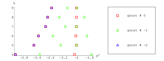
Figure 1: The first group of zeros of $\Delta^{\scriptscriptstyle(n)}_{-}(p^{2})$, for $n=0,-1,-2$ at levels $L=4,\ldots,9$.

$\scriptstyle{\rm(a)}$

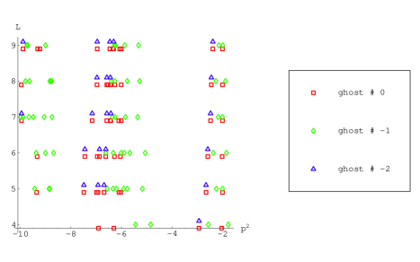
$\scriptstyle{\rm(b)}$

Figure 2: Zeros of $\Delta^{\scriptscriptstyle(n)}_{-}(p^{2})$ (a) and of $\Delta^{\scriptscriptstyle(n)}_{+}(p^{2})$ (b) for $n=0,-1,-2$ at levels $L=4,\ldots,9$ up to $p^{2}=-10$.

In conclusion in the region where it appears that the LT approximation is relatively accurate ($p^{2}\gtrsim-5$) zeros of the determinants only occur in the odd sector: all these zeros are located around $p^{2}\approx-2$ and well separated from any other zeros. Their center of mass is at

$${\bar{m}}^{2}=-2.32,-2.22,-2.19,-2.16,-2.14,-2.13\quad{\rm for}\quad L=4,\ldots,9$$ (58)

and their spreads

$$\Delta m^{2}=0.45,0.27,0.29,0.19,0.22,0.16\qquad{\rm for}\quad L=4,\ldots,9$$ (59)

tend to decrease as the level goes up.

Therefore it is reasonable to conclude that they correspond to a single determinant multiplet. For this group of zeros the Fadeev-Popov index (43) does vanish:

$$I_{FP}({\bar{m}})=d_{0}-2\,d_{1}+2\,d_{2}=2-2\cdot 2+2\cdot 1=0$$ (60)

in agreement with Sen’s conjecture. Note also that the zero of $\Delta^{(-2)}_{-}$ is exactly degenerate with one of the two zeros of $\Delta^{(0)}_{-}$. This is due to the $SU(1,1)$ symmetry we mentioned above. Therefore it is not possible to split the multiplet in Figure 1 into two or more smaller multiplets with non-negative indices: the only way to get a non-negative index is to consider all the zeros as corresponding to degenerate fields carrying no total number of physical degrees of freedom.

4 Relative and Absolute Cohomologies

We already recalled that the number of physical states of open string theory is given by the dimension of the cohomology ${\cal H}^{\scriptscriptstyle(0)}({\widetilde{Q}})$ on ${F}_{\scriptscriptstyle 0}$, the space of states of CFT ghost number 0. Let us also introduce the spaces ${\cal H}^{\scriptscriptstyle(n)}({\widetilde{Q}})$, the ${\widetilde{Q}}$-cohomologies on ${F}_{\scriptscriptstyle n}$, the states of CFT ghost number $n\not=0$: in the following we will refer to the ${\cal H}^{\scriptscriptstyle(n)}({\widetilde{Q}})$’s as the absolute ${\widetilde{Q}}$-cohomologies. Since ${\widetilde{Q}}$ is symmetric with respect to the non-degenerate bilinear form $(\,\cdot\,,\,\cdot)$, the following duality between absolute cohomologies holds

$${\cal H}^{\scriptscriptstyle(n)}({\widetilde{Q}})={\cal H}^{\scriptscriptstyle(1-n)}({\widetilde{Q}})$$ (61)

In the perturbative case, the absolute cohomologies which are non-vanishing (for non-exceptional momenta) are ${\cal H}^{\scriptscriptstyle(0)}(Q)$ — the physical state cohomology — and its dual ${\cal H}^{\scriptscriptstyle(1)}(Q)$. In this section we will probe the non-perturbative cohomologies ${\cal H}^{\scriptscriptstyle(n)}({\widetilde{Q}})$ for $n=-1,-2$ (and their duals) and we will exhibit evidence for their non-emptiness.

One way to compute ${\cal H}^{\scriptscriptstyle(n)}({\widetilde{Q}})$ is based on the preliminary computation of a different kind of ${\widetilde{Q}}$-cohomologies — the relative cohomologies. The ${\widetilde{Q}}$-cohomology of ghost number $n$ relative to $b_{0}$ is defined on the space ${\widetilde{W}}_{\scriptscriptstyle n}$ of states $\phi_{n}$ of ghost number $n$ which are $b_{0}$ and ${\widetilde{L}}_{0}$ invariant:

$$\phi_{n}\in{\widetilde{W}}_{\scriptscriptstyle n}\,\mathrel{\mathop{\iff}^{\rm def}}\,b_{0}\,\phi_{n}={\widetilde{L}}_{0}\,\phi_{n}=0$$ (62)

The relative ${\widetilde{Q}}$-cohomology of ghost number $n$ is given by the ${\widetilde{Q}}$-closed states $\phi_{n}\in{\widetilde{W}}_{\scriptscriptstyle n}$

$${\widetilde{Q}}\,\phi_{n}=0$$ (63)

modulo the states which are in the ${\widetilde{Q}}$ image of ${\widetilde{W}}_{\scriptscriptstyle n-1}$

$$\phi_{\scriptscriptstyle n}\sim\phi^{\prime}_{\scriptscriptstyle n}=\phi_{\scriptscriptstyle n}+{\widetilde{Q}}\,\phi_{\scriptscriptstyle n-1}$$ (64)

where $\phi_{\scriptscriptstyle n-1}\in{\widetilde{W}}_{\scriptscriptstyle n-1}$. Such a definition is consistent since

$$\{{\widetilde{Q}},b_{0}\}={\widetilde{L}}_{0}$$ (65)

The relative cohomologies of ${\widetilde{Q}}$ will be denoted by ${\tilde{\mathrm{h}}}^{\scriptscriptstyle(n)}$.

To unravel the relation between absolute and relative ${\widetilde{Q}}$ cohomologies it is useful to review the same relation for the perturbative $Q$. $Q$ can be decomposed as follows

$$Q=c_{0}\,L_{0}+b_{0}\,D+M$$ (66)

where $L_{0}$, $D$ and $M$ are independent of $c_{0}$ and $b_{0}$. $Q^{2}=0$ implies the relations

$$M^{2}+D\,L_{0}=0\qquad[D,L_{0}]=[L_{0},M]=[M,D]=0$$ (67)

Note that the first of the equations above implies that $M^{2}=0$ on $W_{\scriptscriptstyle n}$, the space of $b_{0}$ and $L_{0}$ invariant states: thus the cohomology of $Q$ relative to $b_{0}$, ${\mathrm{h}}^{\scriptscriptstyle(n)}$, coincides with the cohomology of $M$ on $W_{\scriptscriptstyle n}$. Since $\{Q,b_{0}\}=L_{0}$, $Q$-closed states which are not $L_{0}$-invariant are necessarily $Q$-trivial. Therefore the computation of the absolute cohomology can be restricted, with no loss of generality, to the subspace $V_{\scriptscriptstyle n}$ of the open string state space with $L_{0}=0$. Define the following maps

$$\!\!\!\!\!\!\!\!\!\imath\,:W_{\scriptscriptstyle n}\rightarrow V_{\scriptscriptstyle n}\qquad \imath(\phi_{n})=\phi_{n}$$ (68)

$$\!\!\!\!\!\!\pi\,:V_{\scriptscriptstyle n}\rightarrow W_{\scriptscriptstyle n-1}\qquad \pi(\phi_{n}+c_{0}\phi_{n-1})=\phi_{n-1}$$

$${\cal D}\,:W_{\scriptscriptstyle n-1}\rightarrow W_{\scriptscriptstyle n+1}\qquad {\cal D}(\phi_{n-1})=D\,\phi_{n-1}$$

It is simple to check that $Q\,\imath=\imath\,M$, $M\,\pi=-\pi\,Q$ and $M\,D=D\,M$. Therefore $\imath$, $\pi$ and ${\cal D}$ descend to cohomology maps:

$$\cdots\;{\mathop{\longrightarrow}^{\cal D}}\;{\mathrm{h}}^{\scriptscriptstyle(n)}\;{\mathop{\longrightarrow}^{\imath}}\;{\cal H}^{\scriptscriptstyle(n)}(Q)\;{\mathop{\longrightarrow}^{\pi}}\;{\mathrm{h}}^{\scriptscriptstyle(n-1)}\;{\mathop{\longrightarrow}^{\cal D}}\;{\mathrm{h}}^{\scriptscriptstyle(n+1)}\;{\mathop{\longrightarrow}^{\imath}}\;\cdots$$ (69)

It is straightforward to verify that the sequence of maps above defines a cohomology complex,

$$\imath\,{\cal D}=\pi\,\imath={\cal D}\,\pi=0$$ (70)

and that moreover the cohomology of this complex is trivial:

$${\rm img}\,{\cal D}=\ker\,\imath\qquad{\rm img}\,\imath=\ker\,\pi\qquad{\rm img}\,\pi=\ker\,{\cal D}$$ (71)

The exact long sequence (69) describes the perturbative absolute cohomologies in terms of the relative ones. This is useful since one can establish by other methods that

$${\mathrm{h}}^{\scriptscriptstyle(n)}=\delta_{n,0}\,{\mathrm{h}}^{\scriptscriptstyle(0)}$$ (72)

at non-exceptional momenta. Then the exact long sequence (69) breaks into short ones:

$$0={\mathrm{h}}^{\scriptscriptstyle(-2)}\;{\mathop{\longrightarrow}^{\cal D}}\;{\mathrm{h}}^{\scriptscriptstyle(0)}\;{\mathop{\longrightarrow}^{\imath}}\;{\cal H}^{\scriptscriptstyle(0)}(Q)\;{\mathop{\longrightarrow}^{\pi}}\;{\mathrm{h}}^{\scriptscriptstyle(-1)}=0$$

$$0={\mathrm{h}}^{\scriptscriptstyle(n)}\;{\mathop{\longrightarrow}^{\imath}}\;{\cal H}^{\scriptscriptstyle(n)}(Q)\;{\mathop{\longrightarrow}^{\pi}}\;{\mathrm{h}}^{\scriptscriptstyle(n-1)}=0\qquad{\rm if}\quad n\not=0,1$$ (73)

One proves in this way that

$${\cal H}^{\scriptscriptstyle(0)}(Q)\simeq{\cal H}^{\scriptscriptstyle(1)}(Q)\simeq{\mathrm{h}}^{\scriptscriptstyle(0)}\qquad{\rm and}\qquad{\cal H}^{\scriptscriptstyle(n)}(Q)=0\quad{\rm if}\quad n\not=0,1$$ (74)

Our goal in the rest of this subsection will be to investigate the relation between the non-perturbative ${\tilde{\mathrm{h}}}^{\scriptscriptstyle(n)}$ and ${\cal H}^{\scriptscriptstyle(n)}({\widetilde{Q}})$ along similar lines and to write down the generalization of the long exact sequence (69). We begin by decomposing ${\widetilde{Q}}$ in terms of $b_{0}$ and $c_{0}$:

$${\widetilde{Q}}=c_{0}\,{\widehat{L}}_{0}+b_{0}\,{\widehat{D}}+{\widehat{M}}+c_{0}\,b_{0}\,{\widehat{Z}}$$ (75)

where ${\widehat{L}}_{0}$, ${\widehat{D}}$, ${\widehat{M}}$ and ${\widehat{Z}}$ are independent of $c_{0}$ and $b_{0}$. The crucial difference between the decomposition (75) of the non-perturbative ${\widetilde{Q}}$ and its perturbative analogue (66) is the term proportional to $c_{0}\,b_{0}$, which is absent in the perturbative case. Note that

$${\widetilde{L}}_{0}\equiv\{{\widetilde{Q}},b_{0}\}={\widehat{L}}_{0}+b_{0}\,{\widehat{Z}}\qquad{\widetilde{D}}\equiv\{{\widetilde{Q}},c_{0}\}={\widehat{D}}-c_{0}\,{\widehat{Z}}$$ (76)

and therefore $[{\widetilde{L}}_{0},c_{0}]=[b_{0},{\widetilde{D}}]=-{\widehat{Z}}$, in agreement with the Jacobi identity (33).

It is worth pausing here to remark that the $(b_{0},c_{0})$ expansion of the first quantized BRS operator ${\widetilde{Q}}_{bcft}$ associated with a generic boundary matter conformal field theory coupled to 2d gravity has ${\widehat{Z}}=0$. However even if the non-perturbative tachyonic vacuum of OSFT were described by such a boundary conformal field theory this would not mean, necessarily, that ${\widehat{Z}}=0$ in the expansion (75) for ${\widetilde{Q}}$; it would only imply that ${\widetilde{Q}}$ is conjugate, by means of a linear field redefinition $U$, to an operator ${\widetilde{Q}}_{bcft}$ whose $(b_{0},c_{0})$ expansion has ${\widehat{Z}}=0$. If $U$ commuted with $b_{0}$, the relative complex $({\widetilde{Q}},b_{0})$ would be equivalent to the complex $({\widetilde{Q}}_{bcft},b_{0})$ (and in this case ${\widehat{Z}}=[{\widehat{L}}_{0},X]$): however, in general, we do not know if the field redefinition $U$ that eliminates ${\widehat{Z}}$ also commutes with $b_{0}$. Since we are looking for properties of the relative complex $({\widetilde{Q}},b_{0})$ we must consider the general case in which ${\widehat{Z}}$ is non-trivial. In the following we will elucidate the complications that a non-vanishing ${\widehat{Z}}$ entails for the relationship between absolute and relative cohomologies of ${\widetilde{Q}}$.

The nilpotency of ${\widetilde{Q}}$ leads to equations that replace the perturbative ones (67):

$${\widehat{M}}^{2}+{\widehat{D}}\,{\widehat{L}}_{0}=0\qquad\{{\widehat{M}},{\widehat{Z}}\}+{\widehat{Z}}^{2}=[{\widehat{D}},\,{\widehat{L}}_{0}]$$

$${\widehat{L}}_{0}\,{\widehat{M}}-({\widehat{M}}+{\widehat{Z}})\,{\widehat{L}}_{0}=0\qquad{\widehat{M}}\,{\widehat{D}}-{\widehat{D}}\,({\widehat{M}}+{\widehat{Z}})=0$$ (77)

These equations show that, like in the perturbative case, the $b_{0}$-relative cohomology ${\tilde{\mathrm{h}}}^{\scriptscriptstyle(n)}$ is the cohomology of the operator ${\widehat{M}}$ on ${\widetilde{W}}_{\scriptscriptstyle n}$, the space of states which are $b_{0}$ and ${\widetilde{L}}_{0}$ invariant: indeed, the first of the equations (77) says that ${\widehat{M}}^{2}=0$ on ${\widetilde{W}}_{\scriptscriptstyle n}$, since Eq. (76) ensures that $\phi_{n}\in{\widetilde{W}}_{\scriptscriptstyle n}\Rightarrow{\widehat{L}}_{0}\,\phi_{n}=0$. Moreover the third of the equations (77) guarantee that ${\widehat{M}}:{\widetilde{W}}_{\scriptscriptstyle n}\to{\widetilde{W}}_{\scriptscriptstyle n+1}$. Let us denote by ${\widetilde{V}}_{\scriptscriptstyle n}$ the space of the states which are ${\widetilde{L}}_{0}$ invariant:

$$(\phi_{n}+c_{0}\,\phi_{n-1})\in{\widetilde{V}}_{\scriptscriptstyle n}\,\mathrel{\mathop{\iff}^{\rm def}}\,{\widetilde{L}}_{0}\,(\phi_{n}+c_{0}\,\phi_{n-1})=0$$ (78)

In what follows we will assume that, analogously to the perturbative case, the open string state space of ghost number $n$ decomposes as follows

$${F}_{\scriptscriptstyle n}={\widetilde{V}}_{\scriptscriptstyle n}\oplus{\rm img}({F}_{\scriptscriptstyle n};{\widetilde{L}}_{0})$$ (79)

where ${\rm img}({F}_{\scriptscriptstyle n};{\widetilde{L}}_{0})$ is the image of ${F}_{\scriptscriptstyle n}$ under the map ${\widetilde{L}}_{0}$. The decomposition above would follow from the symmetry of ${\widetilde{L}}_{0}$ with respect to a positive definite bilinear form. However $(\cdot\,,\,\cdot)$ is not positive definite and thus (79) appears to be an independent hypothesis. (79) ensures that, as in the perturbative case, the absolute ${\widetilde{Q}}$-cohomology is contained in the kernel of ${\widetilde{L}}_{0}$, ${\widetilde{V}}_{\scriptscriptstyle n}$.

Let us introduce the immersion and projection maps $\imath$ and $\pi$:

$$\!\!\!\!\!\!\!\!\!\imath\,:{\widetilde{W}}_{\scriptscriptstyle n}\rightarrow{\widetilde{V}}_{\scriptscriptstyle n}\qquad \imath(\phi_{n})=\phi_{n}$$ (80)

$$\!\!\!\!\!\!\pi\,:{\widetilde{V}}_{\scriptscriptstyle n}\rightarrow\check{W}_{\scriptscriptstyle n-1}\qquad \pi(\phi_{n}+c_{0}\phi_{n-1})=\phi_{n-1}$$

where $\check{W}_{\scriptscriptstyle n}$ is the subspace of ${\widetilde{W}}_{\scriptscriptstyle n}$ defined as follows

$$\phi_{n}\in\check{W}_{\scriptscriptstyle n}\,\mathrel{\mathop{\iff}^{\rm def}}\,\phi_{n}\in{\widetilde{W}}_{\scriptscriptstyle n},\,\,{\widehat{Z}}\,\phi_{n}={\widehat{L}}_{0}\,\phi_{n+1},\,\,\phi_{n+1}\in\Omega_{\scriptscriptstyle n+1}$$ (81)

On the space $\Omega_{\scriptscriptstyle n}$ of $b_{0}$-invariant states, the kinetic operator ${\widetilde{L}}_{0}$ of the gauge-fixed open string field theory reduces to ${\widehat{L}}_{0}$. Since $b_{0}$ commutes with ${\widetilde{L}}_{0}$, the decomposition (79) of the total open string state space ${F}_{\scriptscriptstyle n}$ induces the following decomposition of $\Omega_{\scriptscriptstyle n}$ as the sum of a vector in ${\widetilde{W}}_{\scriptscriptstyle n}$, the kernel of ${\widehat{L}}_{0}$, and a vector in the image of ${\widehat{L}}_{0}$ in $\Omega_{\scriptscriptstyle n}$:

$$\Omega_{\scriptscriptstyle n}={\widetilde{W}}_{\scriptscriptstyle n}\oplus{\rm img}(\Omega_{\scriptscriptstyle n};{\widehat{L}}_{0})$$ (82)

Correspondingly one can write the following decomposition for ${\widehat{Z}}$:

$${\widehat{Z}}=\check{Z}+{\widehat{L}}_{0}\,X$$ (83)

where ${\widehat{L}}_{0}\,\check{Z}=0$, and the operator $X:\Omega_{\scriptscriptstyle n}\to\Omega_{\scriptscriptstyle n+1}$ is defined up to an operator whose image is in the kernel of ${\widehat{L}}_{0}$. Therefore the space $\check{W}_{\scriptscriptstyle n}$ defined in Eq. (81) coincides with the kernel of $\check{Z}$ in ${\widetilde{W}}_{\scriptscriptstyle n}$:

$$\check{W}_{\scriptscriptstyle n}=\ker\check{Z}\cap{\widetilde{W}}_{\scriptscriptstyle n}$$ (84)

$\imath$ and $\pi$ define the following exact short sequence:

$$0\;\longrightarrow{\widetilde{W}}_{\scriptscriptstyle n}\;{\mathop{\longrightarrow}^{\imath}}\;{\widetilde{V}}_{\scriptscriptstyle n}\;{\mathop{\longrightarrow}^{\pi}}\;\check{W}_{\scriptscriptstyle n-1}\;\longrightarrow\;0$$ (85)

Note that ${\widetilde{Q}}\,\imath=\imath\,{\widehat{M}}$ and ${\widehat{M}}\,\pi=-\pi\,{\widetilde{Q}}$. Moreover

$${\widehat{M}}:\check{W}_{\scriptscriptstyle n}\to\check{W}_{\scriptscriptstyle n+1}$$ (86)

by virtue of the nilpotency relations (77). To see this, insert the decomposition (83) of ${\widehat{Z}}$ into the second equation in (77):

$$\{{\widehat{M}},\check{Z}\}+\check{Z}^{2}+\{{\widehat{M}}+\check{Z},{\widehat{L}}_{0}\,X\}+({\widehat{L}}_{0}\,X)^{2}=$$

$$=\{{\widehat{M}},\check{Z}\}+\check{Z}^{2}+({\widehat{M}}+{\widehat{Z}})\,{\widehat{L}}_{0}\,X+{\widehat{L}}_{0}\,X\,({\widehat{M}}+\check{Z})=$$

$$=\{{\widehat{M}},\check{Z}\}+\check{Z}^{2}+{\widehat{L}}_{0}\,(\{{\widehat{M}},X\}+X\,\check{Z})=[{\widehat{D}},\,{\widehat{L}}_{0}]$$ (87)

where we used the the third equation in (77). Applying both sides of this equation to ${\widetilde{W}}_{\scriptscriptstyle n-2}$ and decomposing their image in $\Omega_{\scriptscriptstyle n}$ according to (82) one obtains

$$\{{\widehat{M}},\check{Z}\}+\check{Z}^{2}=0\qquad{\widehat{L}}_{0}\,(\{{\widehat{M}},X\}+X\,\check{Z}+{\widehat{D}})=0\qquad{\rm on}\quad{\widetilde{W}}_{\scriptscriptstyle n}$$ (88)

The first of these relations implies that ${\widehat{M}}$ and $\check{Z}$ anti-commutes on $\check{W}_{\scriptscriptstyle n}$, thus Eq. (86) holds.

In conclusion, the following diagram is (anti)-commutative

$$\matrix{0&\smash{\mathop{\longrightarrow}\limits}&{\widetilde{W}}_{\scriptscriptstyle n}&\smash{\mathop{\longrightarrow}\limits^{\imath}}&{\widetilde{V}}_{\scriptscriptstyle n}&\smash{\mathop{\longrightarrow}\limits^{\pi}}&\check{W}_{\scriptscriptstyle n-1}&\smash{\mathop{\longrightarrow}\limits}&0\cr&&\Big{\downarrow}\hbox to0.0pt{$\vbox{\hbox{$\scriptstyle{\widehat{M}}$}}$\hss}&&\Big{\downarrow}\hbox to0.0pt{$\vbox{\hbox{$\scriptstyle{\widetilde{Q}}$}}$\hss}&&\Big{\downarrow}\hbox to0.0pt{$\vbox{\hbox{$\scriptstyle{\widehat{M}}$}}$\hss}\cr 0&\smash{\mathop{\longrightarrow}\limits}&{\widetilde{W}}_{\scriptscriptstyle n+1}&\smash{\mathop{\longrightarrow}\limits^{\imath}}&{\widetilde{V}}_{\scriptscriptstyle n+1}&\smash{\mathop{\longrightarrow}\limits^{\pi}}&\check{W}_{\scriptscriptstyle n}&\smash{\mathop{\longrightarrow}\limits}&0\cr}$$ (89)

We are thus in condition to apply the general theorem of [12]: the short sequence (85) gives rise to the following exact long sequence of ${\widetilde{Q}}$-cohomologies

$$\cdots\;{\mathop{\longrightarrow}^{\widetilde{\cal D}}}\;{\tilde{\mathrm{h}}}^{\scriptscriptstyle(n)}\;{\mathop{\longrightarrow}^{\imath}}\;{\cal H}^{\scriptscriptstyle(n)}({\widetilde{Q}})\;{\mathop{\longrightarrow}^{\pi}}\;{\check{\mathrm{h}}}^{\scriptscriptstyle(n-1)}\;{\mathop{\longrightarrow}^{\widetilde{\cal D}}}\;{\tilde{\mathrm{h}}}^{\scriptscriptstyle(n+1)}\;{\mathop{\longrightarrow}^{\imath}}\;\cdots$$ (90)

This is the non-perturbative generalization of the sequence (69) that we were seeking for. $\widetilde{\cal D}$ is the operator

$$\widetilde{\cal D}\equiv{\widehat{D}}+{\widehat{M}}\,X$$ (91)

and ${\check{\mathrm{h}}}^{\scriptscriptstyle(n)}$ is a new kind of cohomology, the cohomology of ${\widehat{M}}$ on $\check{W}_{\scriptscriptstyle n}$, whose representatives $\phi_{n}$ satisfy the following conditions

$${\widehat{M}}\,\phi_{n}=0,\;\phi_{n}\in\check{W}_{\scriptscriptstyle n},\quad\phi_{n}\sim\phi_{n}+{\widehat{M}}\,\phi_{n-1},\;\phi_{n-1}\in\check{W}_{\scriptscriptstyle n-1}$$ (92)

${\check{\mathrm{h}}}^{\scriptscriptstyle(n)}$ is the same as the cohomology of ${\widehat{M}}$ relative to $\check{Z}$. It is well-defined since ${\widehat{M}}$ sends the kernel of $\check{Z}$ into itself (See Eq. (86)). When $\check{Z}\not=0$, ${\check{\mathrm{h}}}^{\scriptscriptstyle(n)}$ differs, in general, from the relative cohomology ${\tilde{\mathrm{h}}}^{\scriptscriptstyle(n)}$. Therefore, in presence of a non-vanishing $\check{Z}$, one cannot express the absolute ${\widetilde{Q}}$-cohomology only in terms of the relative cohomologies ${\tilde{\mathrm{h}}}^{\scriptscriptstyle(n)}$ — one needs the knowledge of the cohomologies ${\check{\mathrm{h}}}^{\scriptscriptstyle(n)}$ as well. We remarked earlier that when ${\widetilde{Q}}$ is conjugate to a BRS operator with ${\widehat{Z}}=0$ by means of a field redefinition which preserves $b_{0}$, ${\widehat{Z}}$ must be a ${\widehat{L}}_{0}$-commutator. In this case then $\check{Z}=0$ on ${\widetilde{W}}_{\scriptscriptstyle n}$, and ${\check{\mathrm{h}}}^{\scriptscriptstyle(n)}={\tilde{\mathrm{h}}}^{\scriptscriptstyle(n)}$.

4.1 Relations between relative cohomologies

In this subsection we want to investigate the relation between the cohomologies ${\check{\mathrm{h}}}^{\scriptscriptstyle(n)}$ and ${\tilde{\mathrm{h}}}^{\scriptscriptstyle(n)}$ that appear in the non-perturbative long exact sequence (90). This relation will be expressed by the two long exact sequences that are written in Eq. (99) below.

There is an obvious immersion $\iota_{\scriptscriptstyle 1}:{\check{\mathrm{h}}}^{\scriptscriptstyle(n)}\rightarrow{\tilde{\mathrm{h}}}^{\scriptscriptstyle(n)}$ of ${\check{\mathrm{h}}}^{\scriptscriptstyle(n)}$ into ${\tilde{\mathrm{h}}}^{\scriptscriptstyle(n)}$, given by the identity map. In general this immersion is neither injective nor surjective. The kernel of the immersion is represented by vectors $\phi_{n}$ which are trivial in ${\tilde{\mathrm{h}}}^{\scriptscriptstyle(n)}$ but not in ${\check{\mathrm{h}}}^{\scriptscriptstyle(n)}$:

$$\phi_{n}={\widehat{M}}\,\phi_{n-1},\;{\rm with}\;\check{Z}\phi_{n-1}\not=0\quad{\rm and}\;\check{Z}\phi_{n}=0$$ (93)

The cokernel is given by the ${\widehat{M}}$-closed $\phi_{n}$ which are not $\check{Z}$-invariant.

On ${\widetilde{W}}_{\scriptscriptstyle n}$ there exists another nilpotent operator beyond ${\widehat{M}}$: indeed, the first of the relations (88) implies that the operator ${\widehat{M}}+\check{Z}$ is nilpotent on ${\widetilde{W}}_{\scriptscriptstyle n}$. Let us denote the cohomology of ${\widehat{M}}+\check{Z}$ on ${\widetilde{W}}_{\scriptscriptstyle n}$ by ${\cal H}^{\scriptscriptstyle(n)}({\widehat{M}}+\check{Z})$.

The existence of the non-degenerate bilinear form $\langle\cdot\,,\,\cdot\rangle$ on $\Omega_{\scriptscriptstyle-n}\times\Omega_{\scriptscriptstyle n}$ ensures that the kernels ${\widetilde{W}}_{\scriptscriptstyle n}$ of the operators ${\widehat{L}}_{0}$ satisfies the following duality relation

$${\widetilde{W}}_{\scriptscriptstyle n}={\widetilde{W}}_{\scriptscriptstyle-n}$$ (94)

The decomposition (82) guarantees that $\langle\cdot\,,\,\cdot\rangle$ is non-degenerate on ${\widetilde{W}}_{\scriptscriptstyle-n}\times{\widetilde{W}}_{\scriptscriptstyle n}$. The symmetry of ${\widetilde{Q}}$ with respect to the bilinear form $(\,\cdot\,,\,\cdot\,)$ is equivalent to the relations

$${\widehat{L}}_{0}^{\dagger}={\widehat{L}}_{0}\qquad{\widehat{D}}^{\dagger}={\widehat{D}}\qquad{\widehat{M}}^{\dagger}={\widehat{M}}+{\widehat{Z}}\qquad{\widehat{Z}}^{\dagger}=-{\widehat{Z}}$$ (95)

where the dagger denotes the adjoint conjugation with respect to the bilinear form $\langle\cdot\,,\,\cdot\rangle$. Therefore if ${\widehat{Z}}\not=0$, ${\widehat{M}}$ fails to be symmetric: the adjoint of ${\widehat{M}}$ with respect to the bilinear form $\langle\cdot\,,\,\cdot\rangle$ on $\Omega_{\scriptscriptstyle-n}\times\Omega_{\scriptscriptstyle n}$ is ${\widehat{M}}+{\widehat{Z}}$ and the adjoint of ${\widehat{M}}$ with respect to the bilinear form $\langle\cdot\,,\,\cdot\rangle$ on ${\widetilde{W}}_{\scriptscriptstyle-n}\times{\widetilde{W}}_{\scriptscriptstyle n}$ is ${\widehat{M}}+\check{Z}$. Therefore, thanks to Hodge decomposition, the cohomology of ${\widehat{M}}$ at ghost number $n$ is isomorphic to the cohomology of ${\widehat{M}}+\check{Z}$ at ghost number $-n$:

$${\cal H}^{\scriptscriptstyle(n)}({\widehat{M}}+\check{Z})={\tilde{\mathrm{h}}}^{\scriptscriptstyle(-n)}$$ (96)

In the perturbative case, when $\check{Z}=0$, the relation above reduces to the duality between relative cohomology ${\mathrm{h}}^{\scriptscriptstyle(n)}={\mathrm{h}}^{\scriptscriptstyle(-n)}$.

The identity map provides an immersion $\iota_{\scriptscriptstyle 2}$ of the cohomology ${\check{\mathrm{h}}}^{\scriptscriptstyle(n)}$ into ${\cal H}^{\scriptscriptstyle(n)}({\widehat{M}}+\check{Z})$. Again, in general, $\iota_{\scriptscriptstyle 2}$ is neither injective nor surjective. The kernel of $\iota_{\scriptscriptstyle 2}$ is represented by vectors $\phi_{n}=({\widehat{M}}+\check{Z})\,\phi_{n-1}$ with ${\widehat{M}}\,\check{Z}\,\phi_{n-1}=0$ and $\check{Z}\,\phi_{n-1}\not=0$. The cokernel is represented by vectors $\phi_{n}$ with $({\widehat{M}}+\check{Z})\,\phi_{n}=0$ and ${\widehat{M}}\,\phi_{n}\not=0$.

In the following we will derive two exact long sequences of cohomologies which captures the lack of injectivity and surjectivity of the immersions $\iota_{\scriptscriptstyle 1}$ and $\iota_{\scriptscriptstyle 2}$.

Consider the short exact sequence between vector spaces

$$0\;\longrightarrow\check{W}_{\scriptscriptstyle n}\;{\mathop{\longrightarrow}^{\rm Id}}\;{\widetilde{W}}_{\scriptscriptstyle n}\;{\mathop{\longrightarrow}^{\check{Z}}}\;{\rm img}({\widetilde{W}}_{\scriptscriptstyle n};\check{Z})\;\longrightarrow\;0$$ (97)

where ${\rm img}({\widetilde{W}}_{\scriptscriptstyle n};\check{Z})$ is the image of ${\widetilde{W}}_{\scriptscriptstyle n}$ under the map $\check{Z}$. Both ${\widehat{M}}$ and ${\widehat{M}}+\check{Z}$ map ${\rm img}({\widetilde{W}}_{\scriptscriptstyle n};\check{Z})$ into ${\rm img}({\widetilde{W}}_{\scriptscriptstyle n+1};\check{Z})$:

$${\widehat{M}}\,\check{Z}\phi_{n}=-\check{Z}\,({\widehat{M}}+\check{Z})\phi_{n}\in{\rm img}({\widetilde{W}}_{\scriptscriptstyle n+1};\check{Z})$$

$$({\widehat{M}}+\check{Z})\,\check{Z}\phi_{n}=-\check{Z}\,{\widehat{M}}\phi_{n}\in{\rm img}({\widetilde{W}}_{\scriptscriptstyle n+1};\check{Z})$$ (98)

Therefore the cohomologies of both ${\widehat{M}}$ and ${\widehat{M}}+\check{Z}$ are well-defined on the spaces ${\rm img}({\widetilde{W}}_{\scriptscriptstyle n-1};\check{Z})$: these cohomologies will be denoted with ${\hat{\mathrm{h}}}^{\scriptscriptstyle(n)}_{\scriptscriptstyle 1}$ and ${\hat{\mathrm{h}}}^{\scriptscriptstyle(n)}_{\scriptscriptstyle 2}$, respectively.

Thus, on the vector spaces $(\check{W}_{\scriptscriptstyle n},{\widetilde{W}}_{\scriptscriptstyle n},{\rm img}({\widetilde{W}}_{\scriptscriptstyle n};\check{Z}))$ appearing in the short sequence (97) we can consider either the coboundary operators $({\widehat{M}},{\widehat{M}},{\widehat{M}}+\check{Z})$ or the operators $({\widehat{M}},{\widehat{M}}+\check{Z},{\widehat{M}})$. Both triples, together with the short sequence (97), give rise to (anti)-commutative diagrams like that in (89). One concludes that the following two long sequences of cohomologies are exact:

$$\cdots\;{\mathop{\longrightarrow}^{\scriptscriptstyle{\widehat{M}}\check{Z}^{-1}}}\;{\check{\mathrm{h}}}^{\scriptscriptstyle(n)}\;{\mathop{\longrightarrow}^{\iota_{\scriptscriptstyle 1}}}\;{\tilde{\mathrm{h}}}^{\scriptscriptstyle(n)}\;{\mathop{\longrightarrow}^{\scriptscriptstyle\check{Z}}}\;{\hat{\mathrm{h}}}^{\scriptscriptstyle(n+1)}_{\scriptscriptstyle 1}\;{\mathop{\longrightarrow}^{\scriptscriptstyle{\widehat{M}}\check{Z}^{-1}}}\;{\check{\mathrm{h}}}^{\scriptscriptstyle(n+1)}\;{\mathop{\longrightarrow}^{\iota_{\scriptscriptstyle 1}}}\;\cdots$$

$$\cdots\;{\mathop{\longrightarrow}^{\scriptscriptstyle 1+{\widehat{M}}\check{Z}^{-1}}}\;{\check{\mathrm{h}}}^{\scriptscriptstyle(n)}\;{\mathop{\longrightarrow}^{\iota_{\scriptscriptstyle 2}}}\;{\tilde{\mathrm{h}}}^{\scriptscriptstyle(-n)}\;{\mathop{\longrightarrow}^{\scriptscriptstyle\check{Z}}}\;{\hat{\mathrm{h}}}^{\scriptscriptstyle(n+1)}_{\scriptscriptstyle 2}\;{\mathop{\longrightarrow}^{\scriptscriptstyle 1+{\widehat{M}}\check{Z}^{-1}}}\;{\check{\mathrm{h}}}^{\scriptscriptstyle(n+1)}\;{\mathop{\longrightarrow}^{\iota_{\scriptscriptstyle 2}}}\;\cdots$$ (99)

Thus we see that ${\tilde{\mathrm{h}}}^{\scriptscriptstyle(n)}={\check{\mathrm{h}}}^{\scriptscriptstyle(n)}$ only if ${\hat{\mathrm{h}}}^{\scriptscriptstyle(n)}_{\scriptscriptstyle 1}={\hat{\mathrm{h}}}^{\scriptscriptstyle(n+1)}_{\scriptscriptstyle 1}=0$ and ${\tilde{\mathrm{h}}}^{\scriptscriptstyle(n)}={\check{\mathrm{h}}}^{\scriptscriptstyle(-n)}$ only if ${\hat{\mathrm{h}}}^{\scriptscriptstyle(n)}_{\scriptscriptstyle 2}={\hat{\mathrm{h}}}^{\scriptscriptstyle(n+1)}_{\scriptscriptstyle 2}=0$.

Let us remark that ${\hat{\mathrm{h}}}^{\scriptscriptstyle(n)}_{\scriptscriptstyle 1}$ and ${\hat{\mathrm{h}}}^{\scriptscriptstyle(n)}_{\scriptscriptstyle 2}$ satisfy simple duality relations:

$${\hat{\mathrm{h}}}^{\scriptscriptstyle(n)}_{\scriptscriptstyle 1}={\hat{\mathrm{h}}}^{\scriptscriptstyle(1-n)}_{\scriptscriptstyle 1}\qquad{\hat{\mathrm{h}}}^{\scriptscriptstyle(n)}_{\scriptscriptstyle 2}={\hat{\mathrm{h}}}^{\scriptscriptstyle(1-n)}_{\scriptscriptstyle 2}$$ (100)

Indeed, the non-degenerate bilinear form $\langle\cdot\,,\,\cdot\rangle$ on ${\widetilde{W}}_{\scriptscriptstyle-n}\times{\widetilde{W}}_{\scriptscriptstyle n}$ projects to a non-degenerate bilinear form $\langle\!\langle\cdot\,,\,\cdot\rangle\!\rangle$ on ${\rm img}\,({\widetilde{W}}_{\scriptscriptstyle n-1};\check{Z})\times{\rm img}\,({\widetilde{W}}_{\scriptscriptstyle-n};\check{Z})$ defined by

$$\langle\!\langle\phi_{n},\,\phi_{-n+1}\rangle\!\rangle\equiv\langle\phi_{n},\,\check{Z}^{-1}\phi_{-n+1}\rangle$$ (101)

Such a non-degenerate form provides the identification

$${\rm img}\,({\widetilde{W}}_{\scriptscriptstyle n-1};\check{Z})={\rm img}\,({\widetilde{W}}_{\scriptscriptstyle-n};\check{Z})$$ (102)

With respect to $\langle\!\langle\cdot\,,\,\cdot\rangle\!\rangle$, both the operators ${\widehat{M}}$ and ${\widehat{M}}+\check{Z}$ are antisymmetric:

$$\langle\!\langle{\widehat{M}}\phi_{n},\,\phi_{-n}\rangle\!\rangle=\langle{\widehat{M}}\phi_{n},\,\check{Z}^{-1}\phi_{-n}\rangle=\langle\phi_{n},\,({\widehat{M}}+\check{Z})\,\check{Z}^{-1}\phi_{-n}\rangle=$$

$$=-\langle\phi_{n},\,\check{Z}^{-1}\,{\widehat{M}}\phi_{-n}\rangle=-\langle\!\langle\phi_{n},\,{\widehat{M}}\,\phi_{-n}\rangle\!\rangle$$ (103)

and similarly for ${\widehat{M}}+\check{Z}$. Thus the duality relations (100) follow by virtue of Hodge decomposition.

4.2 The numerical data

In this subsection we will start from the numerical computation of the dimensions of ${\widetilde{W}}_{\scriptscriptstyle n}$ in the region of negative $p^{2}$ where the LT approximation appears to be reliable. We will explain that our numerical data imply that for $p^{2}=-{\bar{m}}^{2}$ a certain linear combination of dimensions of relative cohomologies ${\tilde{\mathrm{h}}}^{\scriptscriptstyle(n)}$ (in the odd twist parity sector) is non-vanishing. From ${\cal H}^{\scriptscriptstyle(0)}({\widetilde{Q}})=0$ at $p^{2}=-{\bar{m}}^{2}$ and from the long exact sequence (90), we will derive some linear relations for the absolute cohomologies at ghost numbers $n=-1,-2$ which involve also the relative cohomologies ${\tilde{\mathrm{h}}}^{\scriptscriptstyle(n)}$ and ${\check{\mathrm{h}}}^{\scriptscriptstyle(n)}$. These relations cannot be satisfied by ${\cal H}^{\scriptscriptstyle(-2)}({\widetilde{Q}})={\cal H}^{\scriptscriptstyle(-1)}({\widetilde{Q}})=0$, since not all the ${\tilde{\mathrm{h}}}^{\scriptscriptstyle(n)}$ can vanish. By imposing the constraints among ${\tilde{\mathrm{h}}}^{\scriptscriptstyle(n)}$, ${\check{\mathrm{h}}}^{\scriptscriptstyle(n)}$ and ${\hat{\mathrm{h}}}^{\scriptscriptstyle(n)}_{\scriptscriptstyle 1,2}$ which follow from the sequences (99) and the duality relations (100) derived in the previous subsection, we will be able to determine all possible values for the dimensions of the various cohomologies that entered our discussion. It will turn out that only 3 different solutions for the dimensions of ${\tilde{\mathrm{h}}}^{\scriptscriptstyle(n)}$, ${\check{\mathrm{h}}}^{\scriptscriptstyle(n)}$ and ${\hat{\mathrm{h}}}^{\scriptscriptstyle(n)}_{\scriptscriptstyle 1,2}$ are compatible both with the “experimental” fact that a certain linear combination of dimensions of ${\tilde{\mathrm{h}}}^{\scriptscriptstyle(n)}$ must not vanish and with the constraints that descend from the sequences (90), (99), (100) — and for all three of them ${\cal H}^{\scriptscriptstyle(-2)}({\widetilde{Q}})={\cal H}^{\scriptscriptstyle(-1)}({\widetilde{Q}})=1$.

We saw in the previous section that the numerical computation is consistent with Sen’s conjecture about the vanishing of ${\cal H}^{\scriptscriptstyle(0)}({\widetilde{Q}})$ for all values of $p^{2}$. Assuming then ${\cal H}^{\scriptscriptstyle(0)}({\widetilde{Q}})={\cal H}^{\scriptscriptstyle(1)}({\widetilde{Q}})=0$, the long sequence (90) breaks into the short exact sequence

$$0\;{\mathop{\longrightarrow}^{\pi}}\;{\check{\mathrm{h}}}^{\scriptscriptstyle(-1)}\;{\mathop{\longrightarrow}^{\widetilde{\cal D}}}\;{\tilde{\mathrm{h}}}^{\scriptscriptstyle(1)}\;{\mathop{\longrightarrow}^{\imath}}\;0$$ (104)

and into the two semi-infinite exact sequences

$$\!\!\!\!\!\!\!\!\cdots\;{\mathop{\longrightarrow}^{\pi}}\;{\check{\mathrm{h}}}^{\scriptscriptstyle(-3)}\;{\mathop{\longrightarrow}^{\widetilde{\cal D}}}\;{\tilde{\mathrm{h}}}^{\scriptscriptstyle(-1)}\;{\mathop{\longrightarrow}^{\imath}}\;{\cal H}^{\scriptscriptstyle(-1)}({\widetilde{Q}})\;{\mathop{\longrightarrow}^{\pi}}\;{\check{\mathrm{h}}}^{\scriptscriptstyle(-2)}\;{\mathop{\longrightarrow}^{\widetilde{\cal D}}}\;{\tilde{\mathrm{h}}}^{\scriptscriptstyle(0)}\;{\mathop{\longrightarrow}^{\imath}}\;0$$

$$\!\!\!0\;{\mathop{\longrightarrow}^{\pi}}\;{\check{\mathrm{h}}}^{\scriptscriptstyle(0)}\;{\mathop{\longrightarrow}^{\widetilde{\cal D}}}\;{\tilde{\mathrm{h}}}^{\scriptscriptstyle(2)}\;{\mathop{\longrightarrow}^{\imath}}\;{\cal H}^{\scriptscriptstyle(-1)}({\widetilde{Q}})\;{\mathop{\longrightarrow}^{\pi}}\;{\check{\mathrm{h}}}^{\scriptscriptstyle(1)}\;{\mathop{\longrightarrow}^{\widetilde{\cal D}}}\;{\tilde{\mathrm{h}}}^{\scriptscriptstyle(3)}\;{\mathop{\longrightarrow}^{\imath}}\;\cdots$$

(105)

From (104) one obtains

$${\tilde{\mathrm{h}}}^{\scriptscriptstyle(1)}={\check{\mathrm{h}}}^{\scriptscriptstyle(-1)}$$ (106)

and this should hold for any $p^{2}$ — if Sen’s conjecture is true.

In the region $p^{2}\gtrsim-5$ more detailed information about the cohomologies appearing in the sequences above comes from the LT numerical computation presented in the previous Section.

Let us denote with ${\widetilde{W}}_{\scriptscriptstyle n}^{\scriptscriptstyle\pm}$ the kernels of the matrices ${\widetilde{L}}_{0}={\widehat{L}}_{0}$ on the spaces $\Omega_{\scriptscriptstyle n}^{\scriptscriptstyle(\pm)}(p)$ with even and odd twist parity. For $p^{2}\gtrsim-5$, the even parity spaces ${\widetilde{W}}_{\scriptscriptstyle n}^{\scriptscriptstyle(+)}=\check{W}_{\scriptscriptstyle n}^{\scriptscriptstyle(+)}$ vanish for all $n$ and, hence, so do the even parity relative cohomologies

$${\tilde{\mathrm{h}}}^{\scriptscriptstyle(n)}_{\scriptscriptstyle+}={\check{\mathrm{h}}}^{\scriptscriptstyle(n)}_{\scriptscriptstyle+}=0\qquad\forall\;n$$ (107)

From the sequences (105) it follows that the absolute cohomologies in the even twist sector ${\cal H}^{\scriptscriptstyle(n)}_{\scriptscriptstyle+}({\widetilde{Q}})$ vanish for all ghost numbers:

$${\cal H}^{\scriptscriptstyle(n)}_{\scriptscriptstyle+}({\widetilde{Q}})=0\quad\forall\;n\quad{\rm and}\quad p^{2}\gtrsim-5$$ (108)

In the odd twist parity sector the situation is more interesting. In the region $p^{2}\gtrsim-5$, there is one single value of $p^{2}=-{\bar{m}}^{2}\approx-2.1$ for which the odd twist parity spaces ${\widetilde{W}}_{\scriptscriptstyle n}^{\scriptscriptstyle(-)}$ for $n=0,\pm 1,\pm 2$ do not vanish. For $p^{2}=-{\bar{m}}^{2}$ we obtained for the determinant indices $d_{n}$ the values

$$d_{0}=2,\quad d_{1}=2,\quad d_{2}=1$$ (109)

From our numerical computation we can determine not only the determinant indices (109) but also the dimensions of the kernels of ${\widehat{L}}_{0}$ as functions of $p^{2}$. Let $C^{\scriptscriptstyle(n,-)}_{L}(p)$ be the kinetic quadratic forms (38-39) in the odd twist parity sector, at level L. In Figure 3 we plot the eigenvalues of $C^{\scriptscriptstyle(n,-)}_{9}(p)$ (for $n=0,-1,-2$) that vanish for $p^{2}\approx-{\bar{m}}^{2}$. The eigenvalues of $C^{\scriptscriptstyle(n,-)}(p)$ with $n\not=0$ come in pairs $(\lambda_{n}(p),-\lambda_{n}(p))$: the vanishing of a pair corresponds to a single null eigenstate of ${\widetilde{L}}_{0}^{\scriptscriptstyle(n,-)}$. Figure 3 shows that for $n=0$ there are two different eigenstates of $C^{\scriptscriptstyle(0,-)}_{9}(p)$ whose eigenvalues vanish at two approximately coincident values of $p^{2}$; for $n=-1$, instead, the (approximate) double zero of $\Delta^{\scriptscriptstyle(-1)}_{-}(p^{2})$ corresponds to a single pair of eigenvalues that vanish (approximately) quadratically. In conclusion, the numerical data imply that for $p^{2}=-{\bar{m}}^{2}$

$$\dim{\widetilde{W}}_{\scriptscriptstyle 0}^{\scriptscriptstyle(-)}=2,\quad\dim{\widetilde{W}}_{\scriptscriptstyle\pm 1}^{\scriptscriptstyle(-)}=1,\quad\dim{\widetilde{W}}_{\scriptscriptstyle\pm 2}^{\scriptscriptstyle(-)}=1$$

$$\dim{\widetilde{W}}_{\scriptscriptstyle\pm n}^{\scriptscriptstyle(-)}=0\quad{\rm for}\;n\geq 3$$ (110)

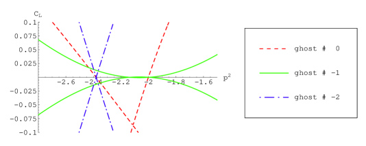
Figure 3: The vanishing eigenvalues of $C^{\scriptscriptstyle(n,-)}_{L}(p)$ for $n=0,-1,-2$ and $p^{2}\approx-2$ at level L=9.

Given the complex ${\widehat{M}}:{\widetilde{W}}_{\scriptscriptstyle n}\rightarrow{\widetilde{W}}_{\scriptscriptstyle n+1}$, one has the following relation between the dimensions of ${\widetilde{W}}_{\scriptscriptstyle n}$ and the dimensions of the cohomologies of ${\widehat{M}}$:

$$\sum_{n=-\infty}^{\infty}(-1)^{n}\,\dim\,{\widetilde{W}}_{\scriptscriptstyle n}=\sum_{n=-\infty}^{\infty}(-1)^{n}\,{\tilde{\mathrm{n}}}^{\scriptscriptstyle(n)}_{\scriptscriptstyle-}$$ (111)

where

$${\tilde{\mathrm{n}}}^{\scriptscriptstyle(n)}_{\scriptscriptstyle-}\equiv\dim{\tilde{\mathrm{h}}}^{\scriptscriptstyle(n)}_{\scriptscriptstyle-}$$ (112)

Therefore our numerical finding (110) implies the relation

$${\tilde{\mathrm{n}}}^{\scriptscriptstyle(-2)}_{\scriptscriptstyle-}-{\tilde{\mathrm{n}}}^{\scriptscriptstyle(-1)}_{\scriptscriptstyle-}+{\tilde{\mathrm{n}}}^{\scriptscriptstyle(0)}_{\scriptscriptstyle-}-{\tilde{\mathrm{n}}}^{\scriptscriptstyle(1)}_{\scriptscriptstyle-}+{\tilde{\mathrm{n}}}^{\scriptscriptstyle(2)}_{\scriptscriptstyle-}=2$$ (113)

Moreover the semi-infinite exact sequences (105) break up at $p^{2}=-{\bar{m}}^{2}$ into finite sequences

$$0\;{\mathop{\longrightarrow}^{\widetilde{\cal D}}}\;{\tilde{\mathrm{h}}}^{\scriptscriptstyle(-1)}_{\scriptscriptstyle-}\;{\mathop{\longrightarrow}^{\imath}}\;{\cal H}^{\scriptscriptstyle(-1)}_{\scriptscriptstyle-}({\widetilde{Q}})\;{\mathop{\longrightarrow}^{\pi}}\;{\check{\mathrm{h}}}^{\scriptscriptstyle(-2)}_{\scriptscriptstyle-}\;{\mathop{\longrightarrow}^{\widetilde{\cal D}}}\;{\tilde{\mathrm{h}}}^{\scriptscriptstyle(0)}_{\scriptscriptstyle-}\;{\mathop{\longrightarrow}^{\imath}}\;0$$

$$0\;{\mathop{\longrightarrow}^{\pi}}\;{\check{\mathrm{h}}}^{\scriptscriptstyle(0)}_{\scriptscriptstyle-}\;{\mathop{\longrightarrow}^{\widetilde{\cal D}}}\;{\tilde{\mathrm{h}}}^{\scriptscriptstyle(2)}_{\scriptscriptstyle-}\;{\mathop{\longrightarrow}^{\imath}}\;{\cal H}^{\scriptscriptstyle(-1)}_{\scriptscriptstyle-}({\widetilde{Q}})\;{\mathop{\longrightarrow}^{\pi}}\;{\check{\mathrm{h}}}^{\scriptscriptstyle(1)}_{\scriptscriptstyle-}\;{\mathop{\longrightarrow}^{\widetilde{\cal D}}}\;0$$

$$0\;{\mathop{\longrightarrow}^{\widetilde{\cal D}}}\;{\tilde{\mathrm{h}}}^{\scriptscriptstyle(-2)}_{\scriptscriptstyle-}\;{\mathop{\longrightarrow}^{\imath}}\;{\cal H}^{\scriptscriptstyle(-2)}_{\scriptscriptstyle-}({\widetilde{Q}})\;{\mathop{\longrightarrow}^{\pi}}\;0$$

$$0\;{\mathop{\longrightarrow}^{\imath}}\;{\cal H}^{\scriptscriptstyle(-2)}_{\scriptscriptstyle-}({\widetilde{Q}})\;{\mathop{\longrightarrow}^{\pi}}\;{\check{\mathrm{h}}}^{\scriptscriptstyle(2)}_{\scriptscriptstyle-}\;{\mathop{\longrightarrow}^{\widetilde{\cal D}}}\;0$$ (114)

Hence, we obtain

$${\cal H}^{\scriptscriptstyle(-2)}_{\scriptscriptstyle-}({\widetilde{Q}})={\tilde{\mathrm{h}}}^{\scriptscriptstyle(-2)}_{\scriptscriptstyle-}={\check{\mathrm{h}}}^{\scriptscriptstyle(2)}_{\scriptscriptstyle-}$$ (115)

from the last two sequences above, while the first two give

$$\dim{\cal H}^{\scriptscriptstyle(-1)}_{\scriptscriptstyle-}({\widetilde{Q}})={\tilde{\mathrm{n}}}^{\scriptscriptstyle(-1)}_{\scriptscriptstyle-}+{\check{\mathrm{n}}}^{\scriptscriptstyle(-2)}_{\scriptscriptstyle-}-{\tilde{\mathrm{n}}}^{\scriptscriptstyle(0)}_{\scriptscriptstyle-}$$

$$\dim{\cal H}^{\scriptscriptstyle(-1)}_{\scriptscriptstyle-}({\widetilde{Q}})=-{\check{\mathrm{n}}}^{\scriptscriptstyle(0)}_{\scriptscriptstyle-}+{\tilde{\mathrm{n}}}^{\scriptscriptstyle(2)}_{\scriptscriptstyle-}+{\check{\mathrm{n}}}^{\scriptscriptstyle(1)}_{\scriptscriptstyle-}$$ (116)

where

$${\check{\mathrm{n}}}^{\scriptscriptstyle(n)}_{\scriptscriptstyle-}\equiv\dim{\check{\mathrm{h}}}^{\scriptscriptstyle(n)}_{\scriptscriptstyle-}$$ (117)

We now want to look for solutions of the equations (113-116) with

$${\tilde{\mathrm{n}}}^{\scriptscriptstyle(0)}_{\scriptscriptstyle-},{\check{\mathrm{n}}}^{\scriptscriptstyle(0)}_{\scriptscriptstyle-}=0,1,2,\qquad{\tilde{\mathrm{n}}}^{\scriptscriptstyle(1)}_{\scriptscriptstyle-},{\check{\mathrm{n}}}^{\scriptscriptstyle(1)}_{\scriptscriptstyle-},{\tilde{\mathrm{n}}}^{\scriptscriptstyle(2)}_{\scriptscriptstyle-},{\check{\mathrm{n}}}^{\scriptscriptstyle(2)}_{\scriptscriptstyle-}=0,1$$ (118)

and

$${\check{\mathrm{n}}}^{\scriptscriptstyle(-2)}_{\scriptscriptstyle-}\leq{\tilde{\mathrm{n}}}^{\scriptscriptstyle(-2)}_{\scriptscriptstyle-}\quad{\rm and}\quad{\check{\mathrm{n}}}^{\scriptscriptstyle(2)}_{\scriptscriptstyle-}\geq{\tilde{\mathrm{n}}}^{\scriptscriptstyle(2)}_{\scriptscriptstyle-}$$ (119)

The last inequalities stem from the fact that ${\widetilde{W}}_{\scriptscriptstyle-3}={\widetilde{W}}_{\scriptscriptstyle 3}=0$.

It is interesting that these equations imply that the absolute cohomologies ${\cal H}^{\scriptscriptstyle(n)}({\widetilde{Q}})$ cannot be vanishing for all $n$. Indeed, if ${\cal H}^{\scriptscriptstyle(-1)}_{\scriptscriptstyle-}({\widetilde{Q}})={\cal H}^{\scriptscriptstyle(-2)}_{\scriptscriptstyle-}({\widetilde{Q}})=0$, the sequences (114) give

$${\tilde{\mathrm{n}}}^{\scriptscriptstyle(-1)}_{\scriptscriptstyle-}={\check{\mathrm{n}}}^{\scriptscriptstyle(1)}_{\scriptscriptstyle-}={\tilde{\mathrm{n}}}^{\scriptscriptstyle(-2)}_{\scriptscriptstyle-}={\check{\mathrm{n}}}^{\scriptscriptstyle(2)}_{\scriptscriptstyle-}=0,\qquad{\tilde{\mathrm{n}}}^{\scriptscriptstyle(0)}_{\scriptscriptstyle-}={\check{\mathrm{n}}}^{\scriptscriptstyle(-2)}_{\scriptscriptstyle-},\qquad{\tilde{\mathrm{n}}}^{\scriptscriptstyle(2)}_{\scriptscriptstyle-}={\check{\mathrm{n}}}^{\scriptscriptstyle(0)}_{\scriptscriptstyle-}$$ (120)

Moreover since ${\tilde{\mathrm{n}}}^{\scriptscriptstyle(0)}_{\scriptscriptstyle-}={\check{\mathrm{n}}}^{\scriptscriptstyle(-2)}_{\scriptscriptstyle-}\leq{\tilde{\mathrm{n}}}^{\scriptscriptstyle(-2)}_{\scriptscriptstyle-}=0$, it follows that ${\tilde{\mathrm{n}}}^{\scriptscriptstyle(0)}_{\scriptscriptstyle-}=0$. Eq. (113) then becomes

$$2=-{\tilde{\mathrm{n}}}^{\scriptscriptstyle(1)}_{\scriptscriptstyle-}+{\tilde{\mathrm{n}}}^{\scriptscriptstyle(2)}_{\scriptscriptstyle-}$$ (121)

which does not admit any solution for ${\tilde{\mathrm{n}}}^{\scriptscriptstyle(1)}_{\scriptscriptstyle-}$ and ${\tilde{\mathrm{n}}}^{\scriptscriptstyle(2)}_{\scriptscriptstyle-}$ in the range (118).

To investigate the possible solutions of our relations let us first consider all possible values of

$${\bf\tilde{n}}\equiv({\tilde{\mathrm{n}}}^{\scriptscriptstyle(-2)}_{\scriptscriptstyle-},{\tilde{\mathrm{n}}}^{\scriptscriptstyle(-1)}_{\scriptscriptstyle-},{\tilde{\mathrm{n}}}^{\scriptscriptstyle(0)}_{\scriptscriptstyle-},{\tilde{\mathrm{n}}}^{\scriptscriptstyle(1)}_{\scriptscriptstyle-},{\tilde{\mathrm{n}}}^{\scriptscriptstyle(2)}_{\scriptscriptstyle-})$$ (122)

in the range (118) satisfying (113). ${\check{\mathrm{n}}}^{\scriptscriptstyle(-2)}_{\scriptscriptstyle-}$ can be either 0 or 1. Suppose first that ${\check{\mathrm{n}}}^{\scriptscriptstyle(-2)}_{\scriptscriptstyle-}=0$. The first equation in (116) becomes $\dim{\cal H}^{\scriptscriptstyle(-1)}_{\scriptscriptstyle-}({\widetilde{Q}})={\tilde{\mathrm{n}}}^{\scriptscriptstyle(-1)}_{\scriptscriptstyle-}-{\tilde{\mathrm{n}}}^{\scriptscriptstyle(0)}_{\scriptscriptstyle-}$. There are only two values for ${\bf\tilde{n}}$ for which ${\tilde{\mathrm{n}}}^{\scriptscriptstyle(-1)}_{\scriptscriptstyle-}-{\tilde{\mathrm{n}}}^{\scriptscriptstyle(0)}_{\scriptscriptstyle-}\geq 0$ and these are $(1,0,0,0,1)$ and $(1,1,1,0,1)$: for both of them $\dim{\cal H}^{\scriptscriptstyle(-1)}_{\scriptscriptstyle-}({\widetilde{Q}})=0$. If $\dim{\cal H}^{\scriptscriptstyle(-1)}_{\scriptscriptstyle-}({\widetilde{Q}})=0$ the first two sequences in (116) split into shorter ones and give

$${\tilde{\mathrm{n}}}^{\scriptscriptstyle(-1)}_{\scriptscriptstyle-}={\check{\mathrm{n}}}^{\scriptscriptstyle(1)}_{\scriptscriptstyle-}=0\qquad{\tilde{\mathrm{n}}}^{\scriptscriptstyle(0)}_{\scriptscriptstyle-}={\check{\mathrm{n}}}^{\scriptscriptstyle(-2)}_{\scriptscriptstyle-}\qquad{\tilde{\mathrm{n}}}^{\scriptscriptstyle(2)}_{\scriptscriptstyle-}={\check{\mathrm{n}}}^{\scriptscriptstyle(0)}_{\scriptscriptstyle-}$$ (123)

Therefore only

$${\bf\tilde{n}}=(1,0,0,0,1)$$ (124)

is allowed, and for this solution we also have

$${\bf\check{n}}\equiv({\check{\mathrm{n}}}^{\scriptscriptstyle(-2)}_{\scriptscriptstyle-},{\check{\mathrm{n}}}^{\scriptscriptstyle(-1)}_{\scriptscriptstyle-},{\check{\mathrm{n}}}^{\scriptscriptstyle(0)}_{\scriptscriptstyle-},{\check{\mathrm{n}}}^{\scriptscriptstyle(1)}_{\scriptscriptstyle-},{\check{\mathrm{n}}}^{\scriptscriptstyle(2)}_{\scriptscriptstyle-})=(0,0,1,0,1)$$ (125)

thanks to (106), (115) and (123).

Consider now the case ${\check{\mathrm{n}}}^{\scriptscriptstyle(-2)}_{\scriptscriptstyle-}=1$. The first equation in (116) becomes $\dim{\cal H}^{\scriptscriptstyle(-1)}_{\scriptscriptstyle-}({\widetilde{Q}})={\tilde{\mathrm{n}}}^{\scriptscriptstyle(-1)}_{\scriptscriptstyle-}-{\tilde{\mathrm{n}}}^{\scriptscriptstyle(0)}_{\scriptscriptstyle-}+1$. There are seven values of ${\bf\tilde{n}}$ in the range (118-119) for which the dimension of ${\cal H}^{\scriptscriptstyle(-1)}_{\scriptscriptstyle-}({\widetilde{Q}})$ is non-negative: five of them have $\dim{\cal H}^{\scriptscriptstyle(-1)}_{\scriptscriptstyle-}({\widetilde{Q}})=0$ and two have $\dim{\cal H}^{\scriptscriptstyle(-1)}_{\scriptscriptstyle-}({\widetilde{Q}})=1$. Among the solutions with vanishing ${\cal H}^{\scriptscriptstyle(-1)}_{\scriptscriptstyle-}({\widetilde{Q}})$ only two are consistent with the relation (123) which derives from ${\cal H}^{\scriptscriptstyle(-1)}_{\scriptscriptstyle-}({\widetilde{Q}})=0$. They are given by

$${\bf\tilde{n}}=(1,0,1,0,0)\qquad{\rm with}\quad{\bf\check{n}}=(1,0,0,0,1)$$ (126)

$${\bf\tilde{n}}=(1,0,1,1,1)\qquad{\rm with}\quad{\bf\check{n}}=(1,1,1,0,1)$$ (127)

For the two values of ${\bf\tilde{n}}$ for which the dimension of ${\cal H}^{\scriptscriptstyle(-1)}_{\scriptscriptstyle-}({\widetilde{Q}})$ is 1, the second equation in (116) gives ${\check{\mathrm{n}}}^{\scriptscriptstyle(0)}_{\scriptscriptstyle-}={\check{\mathrm{n}}}^{\scriptscriptstyle(1)}_{\scriptscriptstyle-}=0,1$. Therefore to each of these two values of ${\bf\tilde{n}}$ there correspond two possible values for ${\bf\check{n}}$:

$${\bf\tilde{n}}=(1,0,0,0,1)\qquad{\rm with}\quad{\bf\check{n}}=(1,0,0,0,1)$$ (128)

$${\bf\tilde{n}}=(1,0,0,0,1)\qquad{\rm with}\quad{\bf\check{n}}=(1,0,1,1,1)$$ (129)

$${\bf\tilde{n}}=(1,1,1,0,1)\qquad{\rm with}\quad{\bf\check{n}}=(1,0,0,0,1)$$ (130)

$${\bf\tilde{n}}=(1,1,1,0,1)\qquad{\rm with}\quad{\bf\check{n}}=(1,0,1,1,1)$$ (131)

Finally, for each of the seven values of ${\bf\tilde{n}}$ and ${\bf\check{n}}$ listed in Eqs. (124-131) we can compute the dimensions of ${\hat{\mathrm{h}}}^{\scriptscriptstyle(n)}_{\scriptscriptstyle 1,2}$ via the sequences (99). It turns out that Eq. (124-125), Eq. (126) and Eq. (130) give rise to values for the dimensions of ${\hat{\mathrm{h}}}^{\scriptscriptstyle(n)}_{\scriptscriptstyle 1,2}$ which are not consistent with the duality relations (100). Moreover, Eq. (127) leads to $\dim{\hat{\mathrm{h}}}^{\scriptscriptstyle(-1)}_{\scriptscriptstyle 1}=1$. This implies that the dimension of ${\rm img}({\widetilde{W}}_{\scriptscriptstyle-2};\check{Z})$ is 1 and thus $\dim\check{W}_{\scriptscriptstyle-2}=0$: but this is inconsistent with the fact that ${\check{\mathrm{n}}}^{\scriptscriptstyle(-2)}_{\scriptscriptstyle-}=1$ in (127).

In conclusion no solution with ${\cal H}^{\scriptscriptstyle(-1)}_{\scriptscriptstyle-}({\widetilde{Q}})=0$ is allowed. There are only three acceptable values for ${\bf\tilde{n}}$ and ${\bf\check{n}}$, those listed in (128), (129) and (131): for all of them

$$\dim{\cal H}^{\scriptscriptstyle(-1)}_{\scriptscriptstyle-}({\widetilde{Q}})=\dim{\cal H}^{\scriptscriptstyle(-2)}_{\scriptscriptstyle-}({\widetilde{Q}})=1\qquad{\rm at}\quad p^{2}=-{\bar{m}}^{2}\approx-2.1$$ (132)

Among the three solutions, there is one, listed in (128), for which ${\tilde{\mathrm{h}}}^{\scriptscriptstyle(n)}={\tilde{\mathrm{h}}}^{\scriptscriptstyle(-n)}={\check{\mathrm{h}}}^{\scriptscriptstyle(n)}$, for any $n$; thus this solution is consistent with $\check{Z}=0$, and with the possibility that the ${\widetilde{Q}}$ be related to a BRS operator with vanishing ${\widehat{Z}}$ by a field redefinition which preserves Siegel gauge. The other two solutions have necessarily $\check{Z}$ and thus ${\widehat{Z}}$ different than zero.

5 BRS Cohomologies without Gauge-Fixing

In this Section we derive a relation between the cohomologies ${\cal H}^{\scriptscriptstyle(n)}({\widetilde{Q}})$ at different ghost numbers by looking at the $p^{2}$ dependence of the operator ${\widetilde{Q}}(p)$ acting on the non-gauge-fixed state spaces ${F}_{\scriptscriptstyle n}$. This relation is not implied by any of the sequences that we constructed in the previous Section. The sequences of the previous Section reflect properties of ${\widetilde{Q}}$ at a fixed $p^{2}$. The relation of this Section is instead a consequence of the fact that the cohomology of ${\widetilde{Q}}(p)$ is empty for $p^{2}$ generic and it appears only on surfaces of positive codimension in momentum space. The fact that this relation is indeed satisfied by the solution (132) for the absolute cohomologies that we derived numerically represents an independent check of the consistency of such a solution.

Let us fix in ${F}_{\scriptscriptstyle n}$ a basis $\{v^{\scriptscriptstyle(n)}_{i_{n}}(p)\}$ of vectors of momentum $p$. Let ${\rm{\widetilde{Q}}}^{\scriptscriptstyle(n)}(p)$ be the matrix describing the action of ${\widetilde{Q}}$ on this basis

$${\widetilde{Q}}(p)\,v^{\scriptscriptstyle(n)}_{i_{n}}(p)={\rm{\widetilde{Q}}}^{\scriptscriptstyle(n)}_{i_{n+1}i_{n}}(p)\,v^{\scriptscriptstyle(n+1)}_{i_{n+1}}(p)$$ (133)

The choice of the basis $\{v^{\scriptscriptstyle(n)}_{i_{n}}(p)\}$ is associated with the choice of a positive definite hermitian product with respect to which the basis is orthonormal. Let $\overline{\rm{\widetilde{Q}}}^{\vphantom{A}\atop{\vphantom{a}\atop\!\!\scriptscriptstyle(n)}}\!(p)$ be the matrix which is the hermitian conjugate of ${\rm{\widetilde{Q}}}^{\scriptscriptstyle(n)}(p)$: in the same basis, $\overline{\rm{\widetilde{Q}}}^{\vphantom{A}\atop{\vphantom{a}\atop\!\!\scriptscriptstyle(n)}}\!(p)$ represents the hermitian conjugate of ${\widetilde{Q}}$ with respect to the positive definite hermitian product defined above. Let us remark that the positive definite product associated with the basis $\{v^{\scriptscriptstyle(n)}_{i_{n}}\}$ has nothing to do with the bilinear form $(\cdot\,,\,\cdot)$ with respect to which ${\widetilde{Q}}$ is symmetric. The choice of the basis will play in this Section the role that the choice of gauge had in Section 2.

Our discussion will focus on the hermitian matrix

$$K^{\scriptscriptstyle(n)}(p)\equiv\overline{\rm{\widetilde{Q}}}^{\vphantom{A}\atop{\vphantom{a}\atop\!\!\scriptscriptstyle(n)}}\!(p)\,{\rm{\widetilde{Q}}}^{\scriptscriptstyle(n)}(p),$$ (134)

Let ${\rm V}_{i_{n}j_{n}}$ be an invertible but not necessarily unitary matrix. Under the change of basis

$$v^{\scriptscriptstyle(n)}_{i_{n}}\to\sum_{j_{n}}\,{\rm V}_{i_{n}j_{n}}\,v^{\scriptscriptstyle(n)}_{j_{n}},$$ (135)

$K^{\scriptscriptstyle(n)}$ transforms as

$$K^{\scriptscriptstyle(n)}(p)\to\overline{\rm V}\,\overline{\rm{\widetilde{Q}}}^{\vphantom{A}\atop{\vphantom{a}\atop\!\!\scriptscriptstyle(n)}}\!(p)\,{\overline{\rm V}}^{-1}\,{\rm V}^{-1}\,{\rm{\widetilde{Q}}}^{\scriptscriptstyle(n)}(p)\,{\rm V}$$ (136)

This shows that, although eigenvalues and eigenstates of $K^{\scriptscriptstyle(n)}(p)$ are basis dependent, its kernel is not and it coincides with the kernel of ${\widetilde{Q}}$.

Eigenstates of $K^{\scriptscriptstyle(n)}(p)$ with vanishing eigenvalues are of two types (See Figure 4 (a)): (A) generic null eigenstates whose eigenvalues are zero for all $p^{2}$; (B) eigenstates whose eigenvalues vanish for isolated values of $p^{2}=-m^{2}$. For reasons that we will review momentarily, eigenstates of $K^{\scriptscriptstyle(n)}(p)$ of type (B) are in the cohomology of ${\rm{\widetilde{Q}}}^{\scriptscriptstyle(n)}$ at $p^{2}=-m^{2}$. Eigenstates of $K^{\scriptscriptstyle(n)}(p)$ of type (A) are cohomologically trivial except for those values of $p^{2}$ for which $K^{\scriptscriptstyle(n-1)}(p)$ has eigenstates of type (B). To study the cohomology of ${\widetilde{Q}}$, it is therefore sufficient to determine the number $N^{\scriptscriptstyle(n)}_{B}(p^{2})$ of eigenstates of type (B) of ghost number $n$ whose eigenvalues vanish at a given value of $p^{2}$: the dimension of the cohomology of ${\widetilde{Q}}(p)$ at ghost number $n$ is given by

$$\dim{\cal H}^{\scriptscriptstyle(n)}({\widetilde{Q}}(p))=N^{\scriptscriptstyle(n)}_{B}(p^{2})+N^{\scriptscriptstyle(n-1)}_{B}(p^{2})$$ (137)

Note that the duality relation (61) implies that

$$N^{\scriptscriptstyle(n)}_{B}(p^{2})=N^{\scriptscriptstyle(-n)}_{B}(p^{2})$$ (138)

and thus knowledge of the BRS cohomology at all ghost numbers only requires the computation of $N^{\scriptscriptstyle(n)}_{B}(p^{2})$ for $n\leq 0$.

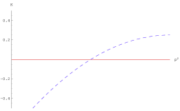
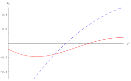
$\scriptstyle{\rm(a)}\hskip 170.71652pt\scriptstyle{\rm(b)}$

Figure 4: Eigenvalues of $K^{\scriptscriptstyle(n)}(p)$ (a) and of level truncated $K^{\scriptscriptstyle(n)}_{L}$ (b) of type (A) (red) and of type (B) (dashed-blue).

Let us briefly review how (137) derives from the continuity of the spectrum of the hermitian and diagonalizable operator $K^{\scriptscriptstyle(n)}(p)$ as a function of $p^{2}$. Nilpotency of ${\widetilde{Q}}$ means

$${\rm{\widetilde{Q}}}^{\scriptscriptstyle(n)}(p)\,{\rm{\widetilde{Q}}}^{\scriptscriptstyle(n-1)}(p)=0,$$ (139)

i.e. the image of ${\rm{\widetilde{Q}}}^{\scriptscriptstyle(n-1)}(p)$ is contained in the kernel of $K^{\scriptscriptstyle(n)}(p)$ for all $p^{2}$. For generic values of $p^{2}$ the image of ${\rm{\widetilde{Q}}}^{\scriptscriptstyle(n-1)}(p)$ also coincides with the kernel of $K^{\scriptscriptstyle(n)}(p)$. At some non-generic value of $p^{2}=-m^{2}$ two things can happen: either a generically non-zero eigenvalue $\lambda(p)$ of $K^{\scriptscriptstyle(n)}(p)$ vanishes at $p^{2}=-m^{2}$ (and the corresponding eigenstate is of type (B)); or some generically trivial eigenstate (of type (A)) becomes non-trivial. In the first case, the type (B) eigenstate can be written as follows

$$\psi_{n}(p)={1\over\sqrt{\lambda(p)}}\,\overline{\rm{\widetilde{Q}}}^{\vphantom{A}\atop{\vphantom{a}\atop\!\!\scriptscriptstyle(n)}}\!(p)\,\psi^{\prime}_{n+1}(p)$$ (140)

where

$$\psi^{\prime}_{n+1}(p)\equiv{1\over\sqrt{\lambda(p)}}\,{\rm{\widetilde{Q}}}^{\scriptscriptstyle(n)}(p)\,\psi_{n}(p)$$ (141)

has unit norm for all $p^{2}$. This shows that $\psi_{n}(p)$ is $\overline{\rm{\widetilde{Q}}}^{\vphantom{A}\atop{\vphantom{a}\atop\!\!\scriptscriptstyle(n-1)}}\!$-closed for any $p^{2}$: moreover for $p^{2}=-m^{2}$, $\psi_{n}(p)$ is also ${\rm{\widetilde{Q}}}^{\scriptscriptstyle(n)}$-closed. This implies that eigenstates of type (B) are cohomologically non-trivial: indeed, a state that is both ${\widetilde{Q}}$-trivial and ${\overline{\widetilde{Q}}}$-closed is orthogonal to itself with respect with the positive hermitian product, and therefore it vanishes. At the same time $\psi^{\prime}_{n+1}(p)$ is an eigenstate of type (A) of $K^{\scriptscriptstyle(n+1)}(p)$: it lies generically in the image of ${\widetilde{Q}}$ and thus it is ${\widetilde{Q}}$-closed for all $p^{2}$. Moreover at $p^{2}=-m^{2}$ it is also ${\overline{\widetilde{Q}}}$-closed and thus it is cohomologically non-trivial at that value of $p^{2}$. Summarizing, eigenvalues of type (B) at ghost number $n$ which vanish at $p^{2}=-m^{2}$ are in one-to-one correspondence with eigenstates of type (A) at ghost number $n+1$ which become non-trivial at the same value of $p^{2}$.

Suppose now that, according to Sen’s hypothesis, ${\cal H}^{\scriptscriptstyle(0)}({\widetilde{Q}})=0$. Then, at a given $p^{2}$, the relation (137) implies

$$0=\dim{\cal H}^{\scriptscriptstyle(-1)}({\widetilde{Q}}(p))-\dim{\cal H}^{\scriptscriptstyle(-2)}({\widetilde{Q}}(p))+\cdots$$ (142)

We saw that for $p^{2}=-{\bar{m}}^{2}\approx-2.1$, $\dim{\cal H}^{\scriptscriptstyle(-n)}({\widetilde{Q}})=0$ for $n\geq 3$. Therefore (142) predicts

$$\dim{\cal H}^{\scriptscriptstyle(-1)}({\widetilde{Q}}(-{\bar{m}}^{2}))=\dim{\cal H}^{\scriptscriptstyle(-2)}({\widetilde{Q}}(-{\bar{m}}^{2}))$$ (143)

in agreement with (132).

5.1 Numerical analysis

The characterization of cohomologically non-trivial states that we explained above leads to a method for the analysis of the BRS cohomology which is completely different than the one of Section 2. The method consists in calculating the number $N_{B}^{\scriptscriptstyle(n)}$ of $K^{\scriptscriptstyle(n)}$ eigenstates of type (B) and using (137) to evaluate the ${\widetilde{Q}}$-cohomology.

The problem, as usual, is that the level truncated BRS operator ${\rm{\widetilde{Q}}}^{\scriptscriptstyle(n)}_{L}(p)$ is only approximately nilpotent. Therefore the eigenvalues of type $(A)$ of $K^{\scriptscriptstyle(n)}(p)$ become, in the LT approximation, generically non-vanishing, and thus a priori indistinguishable from the eigenvalues of type (B) (See Figure 4 (b)). To make use of (137) one must find a way to distinguish among the eigenvalues of $K^{\scriptscriptstyle(n)}_{L}$ those that correspond to eigenvalues of type (A) of the exact $K^{\scriptscriptstyle(n)}(p)$. With this aim, let us observe that for $p^{2}\gg 1$ the non-perturbative ${\widetilde{Q}}(p)$ converges exponentially to the perturbative $Q(p)$. Since LT preserves the nilpotency of $Q(p)$, the eigenvalues of type (A) of $K^{\scriptscriptstyle(n)}(p)$ correspond to eigenvalues of the level truncated $K^{\scriptscriptstyle(n)}_{L}(p)$ which converge to zero for $p^{2}\to\infty$.

In conclusion the method should go as follows: one looks at an eigenvalue $\lambda(p)$ of $K^{\scriptscriptstyle(n)}_{L}(p)$ that vanishes at some $p^{2}=-m^{2}$ and follows it for $p^{2}\gg-m^{2}$ into the region where ${\widetilde{Q}}(p)\approx Q(p)$. If the eigenvalue flows to zero it is of type (A) and thus it does not contribute to $N_{B}^{\scriptscriptstyle(n)}$; we will refer to such eigenvalues as “trivial”. If on the other hand the eigenvalue diverges for $p^{2}\to\infty$ we will call it “non-trivial”: the corresponding eigenstate, for $p^{2}=-m^{2}$ is in the cohomology (of type (B)) of ${\widetilde{Q}}$ at ghost number $n$.

The method presents various technical difficulties. One difficulty is associated with “level crossing” of eigenvalues. Suppose that at some $p_{0}^{2}>-m^{2}$ the eigenvalue $\lambda_{1}(p)$ associated with the eigenstate $\psi_{1}(p)$ crosses another eigenvalue $\lambda_{2}(p)$ corresponding to the eigenstate $\psi_{2}(p)$. For $p^{2}>p_{0}^{2}$ one should be careful to follow the eigenvalue corresponding to the eigenstate which is continuously connected with $\psi_{1}(p)$ for $p^{2}<p_{0}^{2}$. In the numerical situation authentic “level crossing” never occurs. In the numerical approximation “level crossing” appears as in Figure 5 (a): two eigenvalues $\lambda_{1}(p)$ and $\lambda_{2}(p)$ become almost degenerate for $p^{2}\approx p_{0}^{2}$ without ever coinciding; the corresponding eigenstates $\psi_{1}(p)$ and $\psi_{2}(p)$ vary rapidly in the region $p^{2}\approx p_{0}^{2}$ and switch among themselves when going through $p_{0}^{2}$:

$$\psi_{1}(p)\bigr{|}_{p^{2}=p^{2}_{0}-\epsilon}\approx\psi_{2}(p)\bigr{|}_{p^{2}=p^{2}_{0}+\epsilon}$$ (144)

with $\epsilon$ positive and small. To characterize “numerical level crossing” one necessitates a quantitative criterion to decide what “rapid change” of $\psi(p)$ means. For $p^{2}\approx p_{0}^{2}$ the two almost degenerate eigenstates $\psi_{1}(p)$ and $\psi_{2}(p)$ mix approximately only among themselves, and thus they can be written as

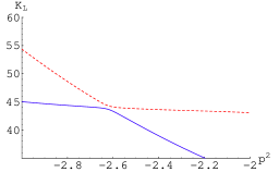
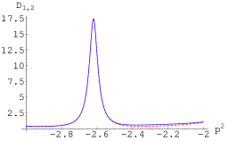
$\scriptstyle{\rm(a)}\hskip 170.71652pt\scriptstyle{\rm(b)}$

Figure 5: (a) Numerical “level crossing” of two eigenvalues of $K^{\scriptscriptstyle(0)}_{L}$ for $L=4$ in the even twist parity sector. (b) The functions $D_{1,2}(p^{2})$ defined in Eq. (146).

$$\psi_{1}(p)=\cos\theta(p)\,e_{1}+\sin\theta(p)\,e_{2}\qquad\psi_{2}(p)=-\sin\theta(p)\,e_{1}+\cos\theta(p)\,e_{2}$$ (145)

where $e_{1}\equiv\psi_{1}(p^{2}_{0}-\epsilon)$ and $e_{2}\equiv\psi_{2}(p^{2}_{0}-\epsilon)$ are orthogonal. Hence the modulus of the derivatives of $\psi_{1}(p)$ and $\psi_{2}(p)$

$$D_{1}(p^{2})\equiv\Bigl{\|}{d\,\psi_{1}(p)\over d\,p^{2}}\Bigr{\|}^{2}\qquad D_{2}(p^{2})\equiv\Bigl{\|}{d\,\psi_{2}(p)\over d\,p^{2}}\Bigr{\|}^{2}$$ (146)

are approximately coincident in the region $p^{2}\approx p_{0}^{2}$

$$D_{1}(p^{2})\approx D_{2}(p^{2})\approx\Bigl{(}{d\,\theta(p)\over d\,p^{2}}\Bigr{)}^{2}$$ (147)

Sharp peaks of the function above can be taken as the signals of “numerical level crossing” (Figure 5 (b)). It is clear that this definition of level crossing involves some arbitrariness: peaks of the function (146) can be more or less sharp corresponding to more or less exact exchange of eigenstates when going through the almost-degeneracy region.

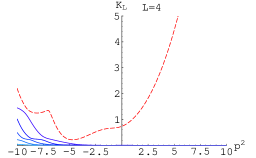
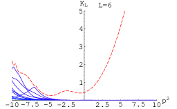
Figure 6: Lowest non-trivial eigenvalue (dashed-red) and trivial eigenvalues of $K^{\scriptscriptstyle(0)}_{L}(p)$ in the even parity sector for $L=4,6$.

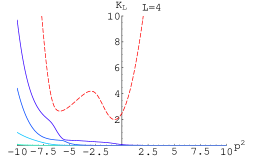
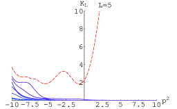
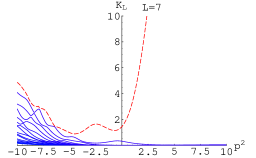
Figure 7: Lowest non-trivial eigenvalue (dashed-red) and trivial eigenvalues of $K^{\scriptscriptstyle(0)}_{L}(p)$ in the odd parity sector for $L=4,5,7$.

Another practical disadvantage of this method is the following: when the level increases BRS nilpotency is more accurate for a wider range of negative $p^{2}$. Hence the zeros of the eigenvalues that are approximately of type (A) become more and more dense on the real (negative) axis. For big enough levels there is not only an ever increasing number of eigenvalues vanishing at some $p^{2}$ to be followed into the perturbative region: also the number of level crossings for each eigenvalue grows rapidly, making progressively more cumbersome to determine if the vanishing eigenvalues are trivial or not. In practice one can more easily determine a region of the $p^{2}$-axis where the non-trivial eigenvalues do not vanish and the numbers $N_{B}^{\scriptscriptstyle(n)}$ are zero.

This method is also not well suited to compute $N_{B}^{\scriptscriptstyle(n)}$ for $n\not=0$. This is so because the level truncated matrix ${\rm{\widetilde{Q}}}^{\scriptscriptstyle(n)}_{L}(p)$ is a square matrix only for $n=0$: for $n<0$ the number of rows is bigger than the number of columns since the number of states of level $L$ and ghost number $n$ is less than the number of states of level $L$ and ghost number $n+1$. For a generic $m\times n$ matrix depending on the parameter $p^{\mu}$ the condition for non-empty kernel determines a sub-manifold of codimension greater than 1 in $p$-space, if $m>n$. Therefore, in the numerical approximation, eigenvalues of $K^{\scriptscriptstyle(n)}_{L}(p)$ never exactly vanish on the $p^{2}$ axis when $n\not=0$: the number $N^{\scriptscriptstyle(n)}_{B}$ should be rather identified with the number of eigenvalues which diverge for $p^{2}\to\infty$ and are “almost” vanishing for some real $p^{2}$ .

In conclusion, the practical relevance of this method is limited to determining the region on the $p^{2}$ axis for which it is safe to say that $N^{\scriptscriptstyle(0)}_{B}$ is zero.

Let us describe the results we obtained. We studied the spectrum of $K^{\scriptscriptstyle(0)}_{L}(p)$ for levels $L=4,5,6,7$, both in the even and the odd twist parity sectors. The numbers of states for each level are reported in Table II. The results of our computations are shown in Figures 6 and 7. The perturbative region for which ${\widetilde{Q}}(p)\approx Q(p)$ is for $p^{2}>10$. The “non-trivial” eigenvalues remain separate from type (A) up to $p^{2}\approx-6$. This excludes cohomology of type (B) of ghost number 0 for $p^{2}>-5$, in agreement with the results of Section 3. The results for ghost numbers -1 and -2 are less transparent. One has also to take into account that there are much less states at these ghost numbers than at ghost number 0: so we expect the LT approximation to be less accurate. The analysis of Section 4 gave $N^{\scriptscriptstyle(-1)}_{B}=0$ and $N^{\scriptscriptstyle(-2)}_{B}=1$ for $p^{2}\approx-2$ in the odd sector. Although we find that there is a “non-trivial” eigenvalue that has a minimum at $p^{2}\approx-2$ it does not seem that this minimum becomes more pronounced as the level is increased (Figure 8).

Level  ghost # 0  ghost # -1  ghost # -2  ghost # -3

 3 (odd) 15 7 1 0

 4 (even) 37 15 2 0

 5 (odd) 75 37 7 0

 6 (even) 150 75 15 1

 7 (odd) 308 160 37 2

Table II: Number of scalar states at various levels.

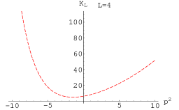
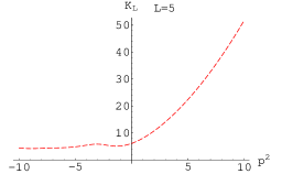
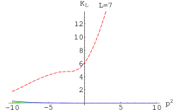
Figure 8: Lowest non-trivial eigenvalue (dashed-red) and trivial eigenvalues of $K^{\scriptscriptstyle(-2)}_{L}(p)$ in the odd parity sector for $L=4,5,7$.

6 Conclusions

In this paper we presented a method for the computation of the number of physical states in OSFT quantized around the tachyonic vacuum, within LT approximation scheme.

We explained why any attempt to compute the BRS cohomology by looking at the kernel of the (approximately nilpotent) level truncated BRS operator ${\widetilde{Q}}$ is plagued by some intrinsic limitations. By such methods one can only compute a certain subset — denoted as “of type B” in the text — of the ghost number 0 cohomology; moreover these methods become more and more inefficient as the level increases.

We thus developed a computational scheme that appears to be better suited to LT approximation. The method focuses on the kinetic operators, ${\widetilde{L}}_{0}^{\scriptscriptstyle(n)}$, of the gauge-fixed OSFT action expanded around the tachyonic vacuum, both in the matter ($n=0$) and in the various ghost ($n\not=0$) sectors. In contrast to the kernel of ${\widetilde{Q}}$, the kernels of ${\widetilde{L}}_{0}^{\scriptscriptstyle(n)}$ are generically empty, as a consequence of gauge-fixing, and acquire a non-vanishing dimension at isolated values of the space-time squared momentum $p^{2}$. For this reason, zeros of $\det{\widetilde{L}}_{0}^{\scriptscriptstyle(n)}$ in the level truncated theory are expected to be stable as the level varies, for those values of $p^{2}$ ($p^{2}\gg-2L$) where LT approximation should apply. We performed a numerical computation of ${\widetilde{L}}_{0}^{\scriptscriptstyle(n)}$ up to level 9, in Siegel gauge and in the scalar sector of the theory: this computation confirmed the expectation above, even if the range of $p^{2}$ where LT approximation seems to be accurate is somewhat smaller than expected: $p^{2}\gtrsim-5$ for $L=9$.

We used the numerical data concerning the vanishing spectrum of ${\widetilde{L}}_{0}^{\scriptscriptstyle(n)}$ in two ways. To begin with, we expressed, by means of the Fadeev-Popov formula, the dimension of the physical state space of OSFT as an index, constructed out of the numbers of zeros of $\det{\widetilde{L}}_{0}^{\scriptscriptstyle(n)}(p)$ weighted with their multiplicities. In the region of $p^{2}$ for which LT approximation is valid, there is a single group of zeros of the determinants $\det{\widetilde{L}}_{0}^{\scriptscriptstyle(n)}(p)$ centered around $p^{2}={\bar{m}}^{2}\approx-2.1$, whose spread decreases as the level goes up, and whose Fadeev-Popov index vanishes. It is reasonable to conclude that this group of zeros corresponds in the exact theory to a multiplet of degenerate matter and ghost fields carrying no physical degree of freedom. This is our numerical evidence confirming Sen’s conjecture that there are no open string states around the tachyonic vacuum.

Assuming that the group of zeros of $\det{\widetilde{L}}_{0}^{\scriptscriptstyle(n)}(p)$ at $p^{2}={\bar{m}}^{2}\approx-2.1$ really corresponds to an exactly degenerate multiplet, we were also able to prove that, at the same $p^{2}$, some of the negative ghost number BRS cohomologies are non-empty: $\dim{\cal H}^{\scriptscriptstyle(-1)}({\widetilde{Q}}(-{\bar{m}}^{2}))=\dim{\cal H}^{\scriptscriptstyle(-2)}({\widetilde{Q}}(-{\bar{m}}^{2}))=1$.

This result derives from two circumstances: first, the dimensions of the kernels of the kinetic operators ${\widetilde{L}}_{0}^{\scriptscriptstyle(n)}$ are connected with the dimensions of the ${\widetilde{Q}}$ cohomologies relative to $b_{0}$; second, the relative ${\widetilde{Q}}$-cohomologies are related to the absolute ${\widetilde{Q}}$-cohomologies ${\cal H}^{\scriptscriptstyle(n)}({{\widetilde{Q}}})$, although we emphasized that this relation, in the non-perturbative case, is considerably more involved than in the perturbative one. In this paper we derived the non-perturbative long exact sequence (Eq. (90)) which connects absolute and relative BRS cohomologies, together with two “sister” long exact sequences involving some new kind of relative BRS cohomologies (Eq. (99)): this is an exact result, independent of the LT approximation.

Let us mention some possible extensions of our work. From a technical point of view, it would be, of course, very useful to improve the accuracy and to extend the $p^{2}$-range of validity of our approximation, both by using more powerful and efficient computational tools and by means of extrapolation algorithms like the ones in [7] and [13]. One should also consider the extension of our computation to the states of higher space-time spin, in particular with the purpose of investigating the gauge field sector of the string theory around the tachyonic vacuum. The main problems to face in order to carry out this program are again of mere computational type.

From a more conceptual point of view, the obvious question that our results raise is the physical meaning of the BRS cohomology at negative ghost numbers. The fact that such cohomology is non-empty is a novel feature of the non-perturbative theory, with respect to the perturbative one; even if it does not contradict the original conjecture of Sen which identifies the tachyonic vacuum with the closed string vacuum, it does not agree with the stronger hypothesis of Vacuum SFT [9], according to which the BRS operator around the tachyonic vacuum has empty cohomology at all ghost numbers.

References

[1]
A. Sen,
“Descent relations among bosonic D-branes,”
Int. J. Mod. Phys. A 14, 4061 (1999) [arXiv:hep-th/9902105].
[2]
A. Sen,
“Universality of the tachyon potential,”
JHEP 9912, 027 (1999) [arXiv:hep-th/9911116].
[3]
E. Witten,
“Noncommutative Geometry And String Field Theory,”
Nucl. Phys. B 268, 253 (1986).
[4]
V. A. Kostelecky and S. Samuel,
“On A Nonperturbative Vacuum For The Open Bosonic String,”
Nucl. Phys. B 336, 263 (1990).
[5]
A. Sen and B. Zwiebach, “Tachyon condensation in string field theory,”
JHEP 0003, 002 (2000) [arXiv:hep-th/9912249].
[6]
N. Moeller and W. Taylor,
“Level truncation and the tachyon in open bosonic string field theory,”
Nucl. Phys. B 583, 105 (2000) [arXiv:hep-th/0002237].
[7]
D. Gaiotto and L. Rastelli,
“Experimental string field theory,”
arXiv:hep-th/0211012.
[8]
I. Ellwood and W. Taylor,
“Open string field theory without open strings,”
Phys. Lett. B 512, 181 (2001)
[arXiv:hep-th/0103085].
[9]
L. Rastelli, A. Sen and B. Zwiebach,
“String field theory around the tachyon vacuum,”
Adv. Theor. Math. Phys. 5, 353 (2002)
[arXiv:hep-th/0012251].
[10]
I. Ellwood, B. Feng, Y. H. He and N. Moeller,
“The identity string field and the tachyon vacuum,”
JHEP 0107, 016 (2001)
[arXiv:hep-th/0105024].
[11]
M. Bochicchio,
“Gauge Fixing For The Field Theory Of The Bosonic String,”
Phys. Lett. B 193, 31 (1987).
C. B. Thorn,
“Perturbation Theory For Quantized String Fields,
Nucl. Phys. B 287, 61 (1987).
[12]
R. Bott and L. W. Tu, “Differential Forms in Algebraic Topology,”
Springer-Verlag, New York, 1997.
[13]
M. Beccaria and C. Rampino,
“Level truncation and the quartic tachyon coupling,”
[arXiv:hep-th/0308059].