Dimensional Reduction of Fermions in
Brane Worlds of the Gross-Neveu Model

Abstract

We study the dimensional reduction of fermions, both in the symmetric and in the broken phase of the 3-d Gross-Neveu model at large $N$. In particular, in the broken phase we construct an exact solution for a stable brane world consisting of a domain wall and an anti-wall. A left-handed 2-d fermion localized on the domain wall and a right-handed fermion localized on the anti-wall communicate with each other through the 3-d bulk. In this way they are bound together to form a Dirac fermion of mass $m$. As a consequence of asymptotic freedom of the 2-d Gross-Neveu model, the 2-d correlation length $\xi=1/m$ increases exponentially with the brane separation. Hence, from the low-energy point of view of a 2-d observer, the separation of the branes appears very small and the world becomes indistinguishable from a 2-d space-time. Our toy model provides a mechanism for brane stabilization: branes made of fermions may be stable due to their baryon asymmetry. Ironically, our brane world is stable only if it has an extreme baryon asymmetry with all states in this “world” being completely filled.

Preprint   HU-EP-03/58,  SFB-CPP-03-40

1 Introduction

Why is gravity so weak? Or equivalently, why are the proton (and other hadrons) so light compared to the Planck scale? As Wilczek has explained nicely [1], the solution to this hierarchy puzzle results from asymptotic freedom. Without any fine-tuning of the bare gauge coupling at distances as short as the Planck length, a 4-d non-Abelian gauge theory like QCD produces a correlation length $\xi$ that is larger than the shortest length scale in the problem, by a factor exponentially large in the inverse coupling. The inverse correlation length defines a mass scale $m=1/\xi$ — the proton mass in Wilczek’s example — that is hence exponentially smaller than the Planck scale. Since we consist mostly of these very light particles (protons and neutrons) in natural units of their mass we experience gravity as a very weak force.

Lattice gauge theorists benefit from the absence of a hierarchy problem in numerical simulations of gauge theories. In this case the shortest length scale (and hence the analog of the Planck length) is the lattice spacing. Again, thanks to asymptotic freedom, without any fine-tuning of the bare gauge coupling, the physical correlation length can be made arbitrarily large in lattice units. Hence, putting aside practical difficulties due to the limited power of computers, there is no problem of principle in approaching the continuum limit in 4-d Yang-Mills theories on the lattice. Unfortunately, the situation is not as simple in full lattice QCD including quarks. In fact, for a long time lattice field theorists have suffered from a hierarchy problem in the fermion sector. This problem arises when one removes the unwanted doubler fermions by breaking chiral symmetry explicitly, for example, by introducing a Wilson term in the lattice fermion action. Recovering chiral symmetry in the continuum limit then requires a delicate fine-tuning of the bare fermion mass. This is not only a pain in practical numerical computations, but should be considered a serious problem of principle at the heart of the nonperturbative regularization of theories with a chiral symmetry. When one works in the continuum, one often takes chiral symmetry for granted because it can be maintained in dimensional regularization. However, the subtleties related to the definition of $\gamma_{5}$ in the framework of dimensional regularization are just another aspect of the same deep problem of chiral symmetry that is obvious on the lattice.

Returning to the hierarchy puzzle, we should ask why the quarks inside the proton are light. In particular, we should still be puzzled by the fact that we consist of not just of gluons, but also of light quarks. Certainly, if one imagines Wilson’s lattice QCD as a (highly simplified) model for the short distance physics of our world, without unnatural fine-tuning, quarks would live at the lattice spacing scale, while gluons (or, more precisely, glueballs) are naturally light. Fortunately, the long-standing hierarchy problem of lattice fermions — and hence of the nonperturbative regularization of chiral symmetry — has recently been solved. Based on work of Callan and Harvey [2], the first step in this direction was taken by Kaplan [3] who realized that massless lattice fermions arise naturally, i.e. without fine-tuning, as zero-modes localized on a domain wall embedded in a higher-dimensional space-time. For example, left-handed fermions in four dimensions can be localized on a domain wall that represents a 3-brane embedded in a 5-d space-time. Similarly, right-handed fermions can be localized on an anti-wall. By keeping the wall and the anti-wall at a sufficiently large distance, i.e. by spatially separating left- and right-handed fermions in the extra dimension, they are prevented from mixing strongly with one another. Thus, they are protected from picking up a large mass and are naturally light. Since $\gamma_{5}$ appears in its action, the 5-d theory itself does not even have a chiral symmetry. Hence, in contrast to four dimensions, a Wilson term in the 5-d lattice action removes the doubler fermions without doing damage to chiral symmetry. Overlap lattice fermions [4] also live in an extra dimension and are closely related to domain wall fermions. When one integrates out the extra dimension, the 4-d version of overlap fermions satisfies the so-called Ginsparg-Wilson relation [5]. As Lüscher first realized, this relation implies a lattice version of chiral symmetry [6] which led him to a spectacular breakthrough: the nonperturbative construction of lattice chiral gauge theories [7]. Perfect and classically perfect lattice fermion actions [8, 9, 10] also obey the Ginsparg-Wilson relation [11]. However, the explicit construction of such actions is a delicate problem that can itself be considered a form of fine-tuning. Fermion actions that naturally obey the Ginsparg-Wilson relation without fine-tuning, on the other hand, can be related to the physics in a higher-dimensional space-time. The existence of light 4-d fermions may hence be a hint to the physical reality of extra dimensions. Indeed, brane worlds embedded in a higher-dimensional space-time provide a very interesting perspective on ordinary 4-d physics [12, 13].

In present lattice QCD applications of domain wall or overlap fermions the extra dimension is not taken physically seriously. In particular, the gluon field is usually frozen in the fifth dimension, thus violating locality in the extra dimension. For left- and right-handed domain wall fermions localized on a wall and an anti-wall, one takes the chiral limit by separating the wall from the anti-wall in the extra dimension, while the gluonic correlation length is kept fixed. Consequently, one approaches the chiral limit before the continuum limit, and the extra dimension does not have a physically meaningful extent. In order to cancel singularities resulting from the 5-d bulk, one introduces ghost fields violating the spin-statistics theorem. While all this is not wrong if one only wants to construct 4-d QCD, it is unnatural if one takes the fifth dimension seriously.

There is an alternative nonperturbative formulation of QCD (and other field theories) — D-theory [14] — in which the extra dimension is used in a more natural way. In D-theory the familiar classical fields emerge dynamically from discrete variables (such as quantum spins or quantum links) which undergo dimensional reduction. In this formulation of QCD, gluons emerge dynamically from higher-dimensional physics. Starting with a 5-d quantum link model from which a non-Abelian Coulomb phase with massless gluons emerges, compactification of the fifth dimension leads to a correlation length (i.e. an inverse glueball mass) that is exponentially large in the size of the extra dimension. As a consequence of asymptotic freedom of 4-d QCD, the size of the extra dimension then shrinks to zero in physical units as one approaches the continuum limit. Domain wall fermions fit naturally into this framework. In particular, the chiral and continuum limits are reached simultaneously, the theory is fully local in the extra dimension, no unphysical ghost fields are needed, and the extra dimension completely disappears in the continuum limit via dimensional reduction. If one imagines the D-theory regularization of QCD as an (again highly simplified) short distance model of our world, not just gluons, but also quarks are naturally light. This solves the second part of the hierarchy puzzle: if we assume the existence of a fifth dimension, we need no longer be puzzled why we also consist of light quarks.

In this paper we use the 3-d Gross-Neveu model [15] at large $N$ as an analytically soluble toy model for illustrating the issues discussed above. Using the standard procedure, domain wall fermions were applied to the Gross-Neveu model in Ref. [16]. In that calculation the fermionic left- and right-handed zero-modes localized on a wall and an anti-wall are coupled by hand. While this is sufficient if one just wants to construct the 2-d Gross-Neveu model, it violates locality in the extra dimension. This is unnatural if one takes that dimension seriously. In this paper, in the spirit of D-theory, we do take the extra dimension physically seriously and let the left- and right-handed zero-modes communicate through the bulk of the extra dimension by a locally implemented 4-fermion interaction. Then, just as in QCD, the D-theory mechanism of dimensional reduction leads to naturally light fermions without fine-tuning. In our calculation not even the domain walls on which fermion states can be localized are put by hand. They arise dynamically from the spontaneous breakdown of the ${\sf Z\!\!\!Z}(2)$ chiral symmetry of the Gross-Neveu model. The walls play the role of branes and hence our construction can be viewed as an attempt to construct stable brane worlds. We find exact brane world solutions just relying on the dynamics of the underlying higher-dimensional theory, without making ad-hoc assumptions about where the branes shall be located. In realistic brane world constructions stabilizing the branes is a highly non-trivial issue. In our model we construct an exact solution for a fully consistent and stable wall-anti-wall configuration. Although our toy model is very simple, it reveals an interesting mechanism for brane stabilization: if branes are made of fermions (and thus have a baryon asymmetry) baryon number conservation in the higher-dimensional theory may imply brane stability. Unfortunately, in our toy “world” the baryon asymmetry is so large that all states are occupied with fermions and any potentially non-trivial physics is completely Pauli-blocked.

In Section 2 basic features of the 2-d Gross-Neveu model are reviewed, while Section 3 discusses the 3-d Gross-Neveu model. In Section 4 the 3-d Gross-Neveu model is considered in the chirally symmetric phase. After compactification of the third dimension, the model undergoes dimensional reduction to the 2-d Gross-Neveu model by the generation of a correlation length that is exponentially large in the size of the extra dimension. Section 5 discusses dimensional reduction from the chirally broken phase of the 3-d model, using configurations with either one wall or a wall-anti-wall pair. In the wall-anti-wall case a naturally light Dirac fermion is generated with its left- and right-handed components being localized on the two walls. Again, the theory undergoes dimensional reduction to the 2-d Gross-Neveu model. The emerging chiral order parameter of the 2-d theory as well as the brane tensions and the issue of brane world stability are also discussed. Finally, Section 6 contains our conclusions. A synopsis of this work is given in Ref. [17].

2 The 2-d Gross-Neveu Model

In this Section, we introduce the 2-d Gross-Neveu model [15] as the target theory which we will later obtain from dimensional reduction of the corresponding 3-d model. Various 2-d field theories, including the Gross-Neveu model, were recently reviewed in [18]. We consider the Gross-Neveu model at large $N$ in the continuum. Its Euclidean action is given by

$$S[\overline{\psi},\psi]=\int d^{2}x\left[\overline{\psi}\gamma_{\mu}\partial_{\mu}\psi-\frac{g}{2N}\left(\overline{\psi}\psi\right)^{2}\right].$$ (2.1)

We have suppressed a flavor index that runs from 1 to $N$ and gives rise to a global $U(N)$ flavor symmetry. The parameter $g$ is the dimensionless 4-fermion coupling which remains fixed in the ’t Hooft limit $N\rightarrow\infty$. The explicit factor $1/N$ ensures that the interaction term stays of the same magnitude as the kinetic term in this limit. In addition to the $U(N)$ flavor symmetry, the model has a ${\sf Z\!\!\!Z}(2)$ chiral symmetry

$$\psi_{L}(x)^{\prime}=\pm\psi_{L}(x),\ \overline{\psi}_{L}(x)^{\prime}=\pm\overline{\psi}_{L}(x),$$

$$\psi_{R}(x)^{\prime}=\mp\psi_{R}(x),\ \overline{\psi}_{R}(x)^{\prime}=\mp\overline{\psi}_{R}(x),$$ (2.2)

where

$$\psi_{R,L}(x)=\frac{1\pm\gamma_{3}}{2}\psi(x),\ \overline{\psi}_{R,L}(x)=\overline{\psi}(x)\frac{1\mp\gamma_{3}}{2}.$$ (2.3)

Let us consider the $N=\infty$ limit and derive a gap equation that describes the spontaneous breakdown of the ${\sf Z\!\!\!Z}(2)$ symmetry of eq.(2). First, we introduce an auxiliary scalar field

$$\phi(x)=\frac{g}{N}\overline{\psi}(x)\psi(x),$$ (2.4)

representing the chiral order parameter $\overline{\psi}\psi$. It linearizes the 4-fermion interaction, such that

$$S[\overline{\psi},\psi,\phi]=\int d^{2}x\left[\overline{\psi}\gamma_{\mu}\partial_{\mu}\psi-\overline{\psi}\psi\phi+\frac{N}{2g}\phi^{2}\right].$$ (2.5)

The partition function then takes the form

$$Z=\int{\cal D}\overline{\psi}{\cal D}\psi\exp(-S[\overline{\psi},\psi])=\int{\cal D}\overline{\psi}{\cal D}\psi{\cal D}\phi\exp(-S[\overline{\psi},\psi,\phi]).$$ (2.6)

In the large $N$ limit we may restrict $\phi(x)$ to a space-time-independent constant $\phi$ [15]. Doing so, the action in momentum space takes the form

$$S[\overline{\psi},\psi,\phi]=\frac{1}{(2\pi)^{2}}\int d^{2}k\ \overline{\psi}(-k)[i\gamma_{\mu}k_{\mu}-\phi]\psi(k)+\frac{NV}{2g}\phi^{2},$$ (2.7)

where $V$ is the volume of space-time. We integrate out the fermion fields

$$\int{\cal D}\overline{\psi}{\cal D}\psi\ \exp(-S[\overline{\psi},\psi,\phi])=\exp(-NVV_{eff}(\phi)),$$ (2.8)

in order to obtain the effective potential $V_{eff}(\phi)$ of the chiral order parameter. In the infinite volume limit the fermion integration yields

$$V_{eff}(\phi)=-\frac{1}{(2\pi)^{2}}\int d^{2}k\ \log\left(k^{2}+\phi^{2}\right)+\frac{1}{2g}\phi^{2}.$$ (2.9)

Using eq.(2.9), the minimum $\phi_{0}$ of the effective potential is determined by

$$\frac{dV_{eff}}{d\phi}(\phi_{0})=-\frac{1}{(2\pi)^{2}}\int d^{2}k\ \frac{2\phi_{0}}{k^{2}+\phi_{0}^{2}}+\frac{\phi_{0}}{g}=0,$$ (2.10)

which implies the gap equation

$$\frac{1}{(2\pi)^{2}}\int d^{2}k\ \frac{2}{k^{2}+\phi_{0}^{2}}=\frac{1}{g}.$$ (2.11)

In order to solve the gap equation, a cut-off $\Lambda_{2}$ is introduced in 2-d momentum space. The ultraviolet limit $\Lambda_{2}\gg\phi_{0}$ is reached for $g\ll 1$ and one then obtains

$$\phi_{0}=m=\Lambda_{2}\exp(-\frac{\pi}{g}).$$ (2.12)

The exponential factor in eq.(2.12) is a manifestation of asymptotic freedom of the 2-d Gross-Neveu model. The factor $\pi$ in the exponent is the inverse of the corresponding 1-loop $\beta$-function coefficient. Due to spontaneous chiral symmetry breaking, the fermions pick up a mass $m=\phi_{0}$. The cut-off $\Lambda_{2}$ is removed by varying the bare coupling $g$ such that the physical fermion mass $m$ remains fixed. After removing the cut-off, the effective potential takes the form

$$V_{eff}(\phi)=\frac{\phi^{2}}{4\pi}(\log\frac{\phi^{2}}{\phi_{0}^{2}}-1),$$ (2.13)

which is depicted in Figure 1.

Figure 1: The effective potential for $d=2$ (with $\phi_{0}=5$).

3 The 3-d Gross-Neveu Model

Next we consider the 3-d Gross-Neveu model [19, 20, 21] with the Euclidean action

$$S[\overline{\Psi},\Psi]=\int d^{3}x\left[\overline{\Psi}\gamma_{\mu}\partial_{\mu}\Psi+\overline{\Psi}\gamma_{3}\partial_{3}\Psi-\frac{G}{2N}\left(\overline{\Psi}\Psi\right)^{2}\right].$$ (3.1)

In three dimensions the 4-fermion coupling $G$ has the dimension of a length. We will soon compactify the third direction or endow it with domain walls and obtain the 2-d Gross-Neveu model by means of dimensional reduction. Hence, in this case, the 3-direction is not Euclidean time but just an additional spatial dimension which will ultimately become invisible. Instead, we choose the 2-direction to represent Euclidean time. In three dimensions there is no chiral symmetry because $\gamma_{3}$ appears explicitly in the action. Still, the 3-d action has a ${\sf Z\!\!\!Z}(2)$ symmetry which reduces to the chiral symmetry of the 2-d Gross-Neveu model after dimensional reduction, but which also involves a spatial inversion in the 3-direction,

$$\Psi_{L}(x_{1},x_{2},x_{3})^{\prime}=\pm\Psi_{L}(x_{1},x_{2},-x_{3}),\ \overline{\Psi}_{L}(x_{1},x_{2},x_{3})^{\prime}=\pm\overline{\Psi}_{L}(x_{1},x_{2},-x_{3}),$$

$$\Psi_{R}(x_{1},x_{2},x_{3})^{\prime}=\mp\Psi_{R}(x_{1},x_{2},-x_{3}),\ \overline{\Psi}_{R}(x_{1},x_{2},x_{3})^{\prime}=\mp\overline{\Psi}_{R}(x_{1},x_{2},-x_{3}).$$ (3.2)

Later we will consider the $x_{3}$-independent zero-mode that determines the physics of the dimensionally reduced 2-d Gross-Neveu model. Then eq.(3) reduces to the usual 2-d ${\sf Z\!\!\!Z}(2)$ chiral symmetry of eq.(2).

As in the 2-d case, we take the large $N$ limit and derive a gap equation

$$\frac{1}{(2\pi)^{3}}\int d^{3}k\ \frac{2}{k^{2}+\Phi_{0}^{2}}=\frac{1}{G}.$$ (3.3)

Introducing a cut-off $\Lambda_{3}$ in 3-d momentum space, and assuming $\Phi_{0}\neq 0$, in the ultraviolet limit $\Lambda_{3}\gg\Phi_{0}$ we obtain

$$\frac{1}{\pi^{2}}(\Lambda_{3}-\frac{\pi}{2}\Phi_{0})=\frac{1}{G}\ \Rightarrow\ \Phi_{0}=2\pi\left(\frac{1}{G_{c}}-\frac{1}{G}\right).$$ (3.4)

We have introduced the critical coupling constant $G_{c}=\pi^{2}/\Lambda_{3}$. At strong coupling, $G>G_{c}$, one has $\Phi_{0}>0$, so we are in the broken phase. For weak coupling, $G<G_{c}$, on the other hand, we are in the symmetric phase. For large $\Lambda_{3}$ (and up to a trivial additive constant) the effective potential reduces to

$$V_{eff}(\Phi)=\frac{1}{6\pi}|\Phi|^{3}-\frac{1}{2}\left(\frac{1}{G_{c}}-\frac{1}{G}\right)\Phi^{2}.$$ (3.5)

In the symmetric phase the effective potential $V_{eff}(\Phi)$ has a single minimum at $\Phi=0$, while in the broken phase it has two degenerate minima at $\Phi=\pm\Phi_{0}$. The effective potential in the symmetric and broken phases is depicted in Figures 2 and 3, respectively.

Figure 2: The effective potential for $d=3$ in the symmetric phase (with $G_{c}=1$ and $G=0.5$).

Figure 3: The effective potential for $d=3$ in the broken phase (with $G_{c}=1$ and $G=2$).

4 Dimensional Reduction from the Chirally Symmetric Phase

In this Section we start from the symmetric phase of the 3-d Gross-Neveu model. By compactifying the third dimension to a circle of circumference $\beta$, the system is dimensionally reduced to the 2-d Gross-Neveu model. Interestingly, the massless fermion that exists in the bulk of the 3-d Gross-Neveu model cannot remain massless after compactification. If it would, the size $\beta$ of the extra dimension would be negligible compared to the then infinite fermionic correlation length, and the model would become a massless 2-d Gross-Neveu model. However, as we have seen, in the 2-d Gross-Neveu model the ${\sf Z\!\!\!Z}(2)$ chiral symmetry is spontaneously broken for all values of the coupling constant $g$. Hence, as the third dimension is compactified, the previously massless 3-d fermion must necessarily pick up a mass. Consequently, its correlation length $\xi=1/m$ will become finite. Then the question arises if $\xi$ is large or small compared to $\beta$.

Let us study the mechanism of dimensional reduction from the symmetric phase in some detail. The 3-d gap equation with periodic boundary conditions in the third direction takes the form

$$\frac{1}{(2\pi)^{3}}\int d^{2}k\ \frac{2\pi}{\beta}\sum_{n\in{\sf Z\!\!\!Z}}\frac{2}{k_{1}^{2}+k_{2}^{2}+(2\pi n/\beta)^{2}+\Phi_{0}^{2}}=\frac{1}{G}.$$ (4.1)

To evaluate the sum, we use the Poisson resummation formula and we obtain

$$\sum_{n\in{\sf Z\!\!\!Z}}\frac{2}{k_{1}^{2}+k_{2}^{2}+(2\pi n/\beta)^{2}+\Phi_{0}^{2}}=\frac{\beta\coth\left(\beta\sqrt{k_{1}^{2}+k_{2}^{2}+\Phi_{0}^{2}}/2\right)}{\sqrt{k_{1}^{2}+k_{2}^{2}+\Phi_{0}^{2}}}.$$ (4.2)

The gap equation then reads

$$\frac{1}{(2\pi)^{2}}\int d^{2}k\ \frac{\coth\left(\beta\sqrt{k_{1}^{2}+k_{2}^{2}+\Phi_{0}^{2}}/2\right)}{\sqrt{k_{1}^{2}+k_{2}^{2}+\Phi_{0}^{2}}}=\frac{1}{G}.$$ (4.3)

Again, we introduce the cut-off $\Lambda_{2}$ in 2-d momentum space and perform the integral. For large $\Lambda_{2}$ we obtain

$$\sinh\frac{\beta\Phi_{0}}{2}=\exp(\pi\beta\left(\frac{\Lambda_{2}}{2\pi}-\frac{1}{G}\right)).$$ (4.4)

In order to match the 2-d cut-off $\Lambda_{2}$ to the 3-d cut-off $\Lambda_{3}$, for a moment we consider the broken phase of the 3-d model. Then $\Phi_{0}$ approaches its constant bulk value as $\beta\rightarrow\infty$, such that eq.(4.4) implies

$$\Phi_{0}=2\pi\left(\frac{\Lambda_{2}}{2\pi}-\frac{1}{G}\right).$$ (4.5)

We match this with the previous result of eq.(3.4) by identifying

$$\frac{\Lambda_{2}}{2\pi}=\frac{1}{G_{c}}=\frac{\Lambda_{3}}{\pi^{2}}.$$ (4.6)

Returning to the symmetric phase of the 3-d model, $\Phi_{0}$ vanishes as $\beta\rightarrow\infty$ and eq.(4.4) implies

$$\xi=\frac{1}{m}=\frac{1}{\Phi_{0}}=\frac{\beta}{2}\exp(\pi\beta\left(\frac{1}{G}-\frac{1}{G_{c}}\right)).$$ (4.7)

Interestingly, the correlation length $\xi$ becomes exponentially larger than $\beta$ as $\beta$ itself goes to infinity. Hence, counter-intuitively, as the size of the third dimension becomes large (in units of the inverse cut-off $1/\Lambda_{3}$) the physical correlation length of the fermion increases exponentially and the low-energy physics reduces to the one of the 2-d Gross-Neveu model. There is a hierarchy of three separate length scales in this problem. The shortest length scale is determined by the inverse cut-off $1/\Lambda_{3}$. The next scale $\beta\gg 1/\Lambda_{3}$ is the size of the extra dimension. Finally, the largest length scale $\xi\gg\beta$ is dynamically generated by spontaneous chiral symmetry breaking in the dimensionally reduced 2-d model. In fact, the size $\beta$ of the extra dimension plays the role of the inverse cut-off for the 2-d Gross-Neveu model that arises by means of dimensional reduction. Identifying the coupling constant of the dimensionally reduced model as

$$\frac{1}{g}=\beta\left(\frac{1}{G}-\frac{1}{G_{c}}\right),$$ (4.8)

eq.(4.7) turns into

$$m=\frac{1}{\xi}=\frac{2}{\beta}\exp(-\frac{\pi}{g}),$$ (4.9)

which is nothing but the asymptotic freedom relation eq.(2.12) of the 2-d Gross-Neveu model. In particular, we identify $2/\beta$ as the effective cut-off of the dimensionally reduced model. The same subtle mechanism of dimensional reduction was first observed in the 3-d $O(3)$ sigma model [22, 23]. However, in that case dimensional reduction results only when one starts in the broken phase of the 3-d model, which contains massless Goldstone bosons. As a consequence of the Mermin-Wagner-Coleman Theorem, these particles cannot remain massless as the theory dimensionally reduces to two dimensions. Since the ${\sf Z\!\!\!Z}(2)$ symmetry of the Gross-Neveu model is discrete, the Theorem does not apply in this case. In the 3-d Gross-Neveu model the massless phase is the one without spontaneous symmetry breaking. Still, both the 2-d $O(3)$ model and the 2-d Gross-Neveu model are massive, although for different reasons. In the next Section we will see how dimensional reduction arises starting from the broken phase of the 3-d Gross-Neveu model. Figure 4 shows the chiral condensate (or equivalently the mass gap) as a function of $G$ both for finite and for infinite $\beta$.

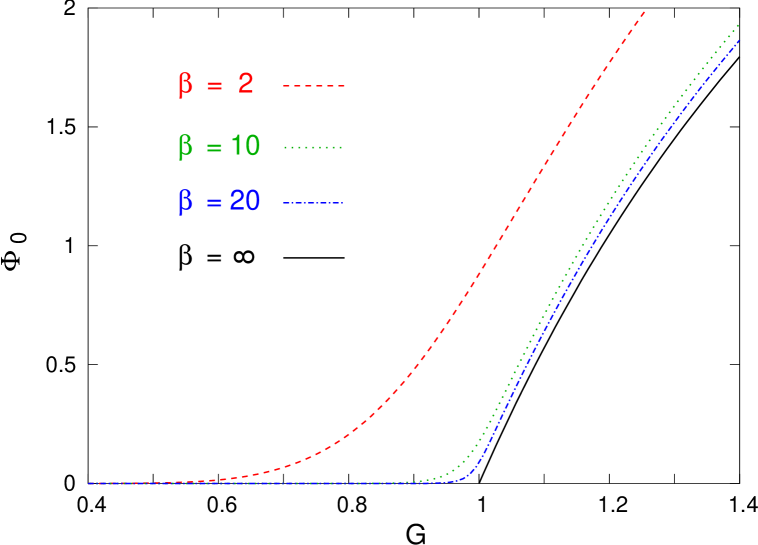
Figure 4: The mass gap for $d=3$ as a function of $G$ at various values of $\beta$ (with $G_{c}=1$).

From the point of view presented in the Introduction, the way we have obtained the 2-d Gross-Neveu model by means of dimensional reduction from the symmetric phase of the 3-d model is not really satisfactory. Since we studied the large $N$ limit, an analytic calculation was possible in the continuum using a momentum cut-off that does not break chiral symmetry explicitly. On the other hand, a fully nonperturbative treatment at finite $N$ would require a formulation on the lattice, which leads to the fermion doubling problem. For even $N$ this problem can be avoided using staggered fermions. However, for odd $N$ one would use Wilson fermions and thus break chiral symmetry explicitly by the regulator. Recovering chiral symmetry in the continuum limit then requires unnatural fine-tuning of the bare fermion mass. The idea of domain wall fermions is to construct naturally light fermions via dimensional reduction from a higher dimension. In the next Section, we will see explicitly how this works in the broken phase of the 3-d Gross-Neveu model. Dimensional reduction from the symmetric phase, on the other hand, requires a 3-d massless fermion to begin with. In a fully nonperturbative lattice calculation at finite $N$ this would require unnatural fine-tuning at the level of the 3-d theory. Hence, the above mechanism of dimensional reduction from the symmetric phase does not work naturally (i.e. without fine-tuning) when the cut-off violates chiral symmetry. This is why we now turn to the chirally broken phase.

5 Dimensional Reduction from the Chirally Broken Phase

In this Section we describe how the 2-d Gross-Neveu model can arise via dimensional reduction from the broken phase of the 3-d model. If one would again compactify the third dimension to a circle, the finite correlation length $\xi=1/m=1/\Phi_{0}$ of the fermion in the 3-d bulk would never become large compared to $\beta$. Hence, with periodic boundary conditions, dimensional reduction would not happen from the broken phase, even in the $\beta\rightarrow 0$ limit, because the ratio $\beta/\xi=\beta\Phi_{0}\rightarrow 2\log(1+\sqrt{2})$ remains non-zero in this limit.

Light fermions in $2n$ dimensions can arise naturally by dimensional reduction from a massive theory in $(2n+1)$ dimensions as zero-modes localized on a domain wall [3]. Interestingly, domain walls indeed exist as stable topological objects in the broken phase of the 3-d Gross-Neveu model. We will see that a system with a single domain wall has a free massless left-handed 2-d fermion living on the wall. A system with a stable wall-anti-wall pair separated by a distance $\beta$, on the other hand, supports a left-handed fermion living on the wall as well as a right-handed fermion living on the anti-wall. The left- and right-handed fermionic zero-modes communicate with each other through the 3-d bulk between the wall and the anti-wall and pick up a mass $m$. Interestingly, in analogy to the mechanism of dimensional reduction discussed before, the corresponding correlation length $\xi=1/m$ grows exponentially with $\beta$ when one separates the wall from the anti-wall. Hence, in units of the 2-d fermion correlation length $\xi$, the size $\beta$ of the bulk between the walls shrinks to zero. Consequently, from the low-energy point of view of a 2-d observer living on the walls, the wall-anti-wall system — although truly 3-dimensional — looks exactly like a 2-d space-time.

5.1 A Brane World with a Single Domain Wall

First we consider a system with a single domain wall separating two distinct broken phases with chiral condensate values $\Phi_{0}$ and $-\Phi_{0}$. The domain wall itself is described by a field configuration $\Phi(x_{3})$ that interpolates between the two vacuum states, $\Phi(\pm\infty)=\pm\Phi_{0}$. Determining the shape $\Phi(x_{3})$ of the domain wall is a non-trivial problem. Fortunately, a similar problem has been solved a long time ago by Dashen, Hasslacher, and Neveu [24] in the 2-d Gross-Neveu model. In that case, the topological object is not a domain wall but simply a solitonic particle. As we will see, the 2-d soliton solution of Ref. [24] naturally extends to three dimensions. In order to determine $\Phi(x_{3})$ we apply the following strategy. First, we make an educated guess (the 2-d soliton solution) for $\Phi(x_{3})$. Second, we integrate out the fermions in the given non-trivial background, and we verify explicitly that the resulting $\overline{\Psi}\Psi$ self-consistently reproduces $\Phi(x_{3})$. Our approach is a 3-d generalization of work by Pausch, Thies, and Dolman [25] and by Feinberg [26], and is also related to work by Chandrasekharan [27].

The ansatz for the domain wall profile which is obvious from what we know about 2-d solitons is given by the standard kink profile

$$\Phi(x_{3})=\Phi_{0}\tanh(\Phi_{0}x_{3}).$$ (5.1)

We have arbitrarily centered the domain wall at $x_{3}=0$. Of course, there is a trivial translational zero-mode which does not concern us here. In Minkowski space-time the fermions propagating in the non-trivial domain wall background field $\Phi(x_{3})$ are described by the single-particle Dirac Hamiltonian

$$H=\gamma_{2}[\gamma_{1}\partial_{1}+\gamma_{3}\partial_{3}-\Phi(x_{3})].$$ (5.2)

We choose the Euclidean Dirac matrices to coincide with the Pauli matrices, $\gamma_{i}=\sigma_{i}$. After dimensional reduction the 1-direction will remain and — from the low-energy point of view of a 2-d observer — the spatial 3-direction becomes invisible. Using translation invariance of the Dirac equation in both, the spatial 1-direction and in time, we make the separation ansatz

$$\Psi(x_{1},x_{3},t)=\Psi(x_{3})\exp(ik_{1}x_{1})\exp(-iEt),$$ (5.3)

which implies

$$\left(\begin{array}[]{cc}k_{1}&i\partial_{3}+i\Phi(x_{3})\\ i\partial_{3}-i\Phi(x_{3})&-k_{1}\end{array}\right)\left(\begin{array}[]{c}\Psi_{R}(x_{3})\\ \Psi_{L}(x_{3})\end{array}\right)=E\left(\begin{array}[]{c}\Psi_{R}(x_{3})\\ \Psi_{L}(x_{3})\end{array}\right).$$ (5.4)

There is a localized state

$$\Psi_{0}(x_{3})=\sqrt{\frac{\Phi_{0}}{2}}\left(\begin{array}[]{c}0\\ \cosh^{-1}(\Phi_{0}x_{3})\end{array}\right),$$ (5.5)

with the energy eigenvalue $E_{0}=-k_{1}>0$. This state describes a free massless left-handed fermion with spatial momentum $k_{1}$ localized on the domain wall. Note that the localized states of positive energy are left-movers with $k_{1}<0$. Since in 2-d there is no spin, a left-handed particle is indeed simply moving to the left. Similarly, the particles localized on an anti-wall with the profile $\Phi(x_{3})=-\Phi_{0}\tanh(\Phi_{0}x_{3})$ are right-movers. The wall profile as well as the wave function of the localized state are illustrated in Figure 5.

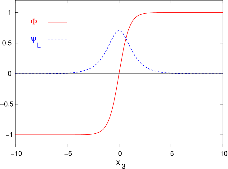
Figure 5: The profile of a single domain wall and the wave function of the left-handed state $\Psi_{0}$ localized on this wall (with $\Phi_{0}=1$).

The spectrum of the Dirac equation also includes a continuum of bulk states

$$\Psi_{k_{3}}(x_{3})=\frac{\exp(ik_{3}x_{3})}{\sqrt{2E(E+k_{1})}}\left(\begin{array}[]{c}i(E+k_{1})\\ \Phi_{0}\tanh(\Phi_{0}x_{3})-ik_{3}\end{array}\right),$$ (5.6)

with the energy eigenvalues $E=\pm\sqrt{k_{1}^{2}+k_{3}^{2}+\Phi_{0}^{2}}$. The localized and bulk states together form a complete orthonormal basis of the single particle Hilbert space.

In the next step, we verify explicitly that the solutions from above self-consistently reproduce the domain wall profile of eq.(5.1). For this purpose we evaluate

$$\overline{\Psi}_{0}(x_{3})\Psi_{0}(x_{3})=\Psi^{\dagger}_{0}(x_{3})\gamma_{2}\Psi_{0}(x_{3})=0,$$

$$\overline{\Psi}_{k_{3}}(x_{3})\Psi_{k_{3}}(x_{3})=-\frac{1}{E}\Phi_{0}\tanh(\Phi_{0}x_{3})=-\frac{1}{E}\Phi(x_{3}).$$ (5.7)

Summing over the filled Dirac sea of negative energy states, in the limit $\Lambda_{2}\gg\Phi_{0}$ one finds

$$\frac{G}{N}\overline{\Psi}(x_{3})\Psi(x_{3})=\Phi(x_{3})\frac{G}{2\pi}\int_{0}^{\Lambda_{2}}\frac{k\,dk}{\sqrt{k^{2}+\Phi_{0}^{2}}}=\Phi(x_{3})\frac{G}{2\pi}(\Lambda_{2}-\Phi_{0})=\Phi(x_{3}),$$ (5.8)

i.e. the ansatz of eq.(5.1) for the profile of the domain wall is indeed reproduced by the actual $\overline{\Psi}\Psi$ of the fermions living in the corresponding background field. The factor $1/N$ has canceled because each negative energy state is filled with $N$ fermions. We have also used eq.(4.5) to eliminate the cut-off $\Lambda_{2}$ in favor of $G$ and $\Phi_{0}$.

Since the modes localized on the wall have $\overline{\Psi}_{0}\Psi_{0}=0$, they have no effect on the self-consistency of the domain wall solution itself. In particular, one can also fill the negative energy states for those modes and thus construct the usual vacuum for the 2-d physics on the brane. By occupying a localized state $\Psi_{0}(x_{3})$ with spatial momentum $-k_{1}$, we then obtain a left-moving particle with energy $E_{0}=-k_{1}$. At low energies $E_{0}\ll\Phi_{0}$ the fermions that are localized on the brane do not feel the extra dimension and see just a 2-d space-time. At sufficiently large energies $E_{0}>\Phi_{0}$, on the other hand, fermions can escape into the extra dimension. From the point of view of a 2-d observer, this process seems to violate fermion number conservation.

At this point we have explicitly constructed a topologically stable brane on which massless left-handed fermions can propagate as free particles. In the case of a single domain wall, the dimensional reduction of fermions from three to two dimensions is straightforward. In the next Subsection we will construct a brane world consisting of a wall-anti-wall pair. In that case, the mechanism of dimensional reduction is more subtle.

5.2 A Brane World Consisting of a Wall-Anti-Wall Pair

As we have seen, left-handed fermions can be localized on a domain wall. Similarly, right-handed fermions can be localized on an anti-wall. A world that contains both left- and right-handed fermions should hence contain a wall-anti-wall pair. In order to keep the fermions light, the wall and the anti-wall must be separated in the extra dimension by a sufficient distance. If the low-energy physics of the dimensionally reduced theory happens simultaneously on the wall and the anti-wall, the question arises how the brane separation $\beta$ compares with the natural length scale $\xi$ on the branes. Interestingly, in analogy to the mechanism of dimensional reduction from the symmetric phase that was discussed in Section 4, we will find that, as $\beta$ increases, the length scale $\xi$ grows exponentially such that the brane separation becomes small in the natural physical units of a low-energy observer.

Again inspired by the corresponding soliton solution of the 2-d Gross-Neveu model, we now make the ansatz

$$\Phi(x_{3})=\Phi_{0}[a\tanh(a\Phi_{0}x_{3}+c)-a\tanh(a\Phi_{0}x_{3}-c)-1].$$ (5.9)

As before, we need to solve the Dirac equation in the given background field. Remarkably, this is still possible in closed form. The following relations are important for the derivation of the results presented below

$$[1+a\tanh(y-c)][1-a\tanh(y+c)]=1-a^{2},$$

$$\frac{\cosh(y+c)}{\cosh(y-c)}=\frac{1}{\sqrt{1-a^{2}}}[1+a\tanh(y-c)],$$

$$\frac{\cosh(y-c)}{\cosh(y+c)}=\frac{1}{\sqrt{1-a^{2}}}[1-a\tanh(y+c)],$$

$$\frac{a}{\cosh(y+c)\cosh(y-c)}=\sqrt{1-a^{2}}[\tanh(y+c)-\tanh(y-c)].$$ (5.10)

Here we have put $a\Phi_{0}x_{3}=y$. The Dirac equation, as well as the above relations, are satisfied only if

$$\tanh(a\Phi_{0}\beta)=\tanh(2c)=a.$$ (5.11)

The parameter $a\in[0,1]$ determines the brane separation $\beta$ and will later be fixed self-consistently. At zero distance we have $a=0$ and hence $\Phi(x_{3})=-\Phi_{0}$, so that we are in one of the two vacua of the 3-d theory. As $a$ approaches 1, on the other hand, $\beta$ goes to infinity. Then $\Phi(x_{3})=\Phi_{0}$ and we are in the other vacuum state of the 3-d theory. Hence, by varying $a$ we can change the brane separation and interpolate smoothly between the two vacua.

In the wall-anti-wall case one obtains the states

$$\Psi_{0}(x_{3})=\frac{\sqrt{a\Phi_{0}}}{2\sqrt{E_{0}(E_{0}+k_{1})}}\left(\begin{array}[]{c}-i(E_{0}+k_{1})\cosh^{-1}(a\Phi_{0}x_{3}-c)\\ m\cosh^{-1}(a\Phi_{0}x_{3}+c)\end{array}\right),$$ (5.12)

localized on the branes. Here

$$m=\sqrt{1-a^{2}}\Phi_{0},$$ (5.13)

is the mass of the particles propagating on the branes and

$$E_{0}=\pm\sqrt{k_{1}^{2}+(1-a^{2})\Phi_{0}^{2}}=\pm\sqrt{k_{1}^{2}+m^{2}},$$ (5.14)

is the corresponding energy. These states describe a Dirac fermion of momentum $k_{1}$ whose left-handed component propagates on the wall, while its right-handed component propagates on the anti-wall. The wall-anti-wall profile, as well as the wave function for the left- and right-handed components of a localized state at rest, are depicted in Figure 6.

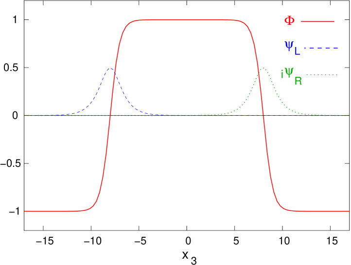
Figure 6: The profile of a wall-anti-wall pair and the left- and right-handed components of a localized state at rest with $k_{1}=0$ (for $\Phi_{0}=1$, $c=8$, i.e. $a=\tanh(16)$).

For a particle moving to the left at high speed one has $E_{0}\approx-k_{1}$. Then the upper component of the wave function, which is localized on the anti-wall, tends to zero, and the particle is almost entirely located on the wall. This is illustrated in Figure 7.

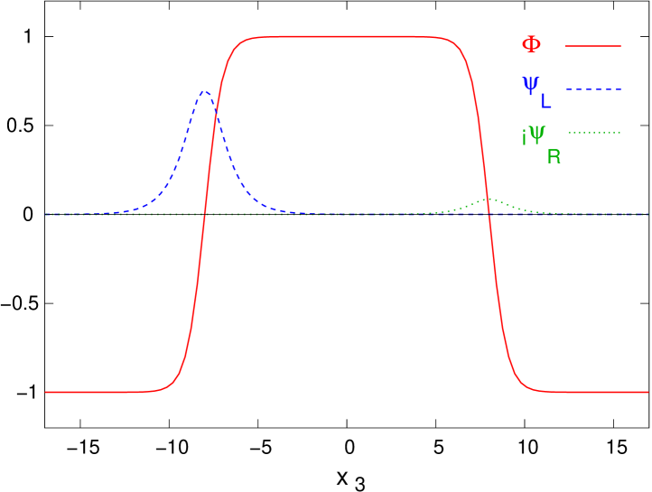
Figure 7: The profile of a wall-anti-wall pair and the left- and right-handed components of a left-moving localized state with $k_{1}=-4m$ (for $\Phi_{0}=1$, $c=8$, i.e. $a=\tanh(16)$).

The wave function of a fast right-mover, on the other hand, is concentrated on the anti-wall.

At $a=0$, i.e. at distance $\beta=0$ between the branes, we end up in the vacuum $\Phi=-\Phi_{0}$ and the mass of the Dirac fermion is simply given by the 3-d fermion mass $m=\Phi_{0}$. When the branes are separated by a large distance $\beta\gg 1/\Phi_{0}$, i.e. for $a\rightarrow 1$, on the other hand, the mass of the Dirac fermion goes to zero as

$$m=2\Phi_{0}\exp(-\beta\Phi_{0}).$$ (5.15)

Consequently, when the branes are separated at a large distance $\beta$, the 2-d correlation length $\xi=1/m\gg\beta$ again grows exponentially with $\beta$ and the system dimensionally reduces. In particular, from the point of view of a low-energy 2-d observer, the left- and right-handed modes propagating simultaneously on the wall and the anti-wall are indistinguishable from an ordinary point-like Dirac fermion. At the same time, a 3-d high-energy observer whose natural length scale is $1/\Phi_{0}$ would say that the Dirac particle consists of a left-handed and a right-handed constituent, both separated by a large distance $\beta\gg 1/\Phi_{0}$.

In the wall-anti-wall configuration the bulk states take the form

$$\Psi_{k_{3}}(x_{3})=\frac{\exp(ik_{3}x_{3})}{\sqrt{2E(E+k_{1})(k_{3}^{2}+a^{2}\Phi_{0}^{2})}}\left(\begin{array}[]{c}i(E+k_{1})[a\Phi_{0}\tanh(a\Phi_{0}x_{3}-c)-ik_{3}]\\ -(\Phi_{0}+ik_{3})[a\Phi_{0}\tanh(a\Phi_{0}x_{3}+c)-ik_{3}]\end{array}\right),$$ (5.16)

with the energy eigenvalues $E=\pm\sqrt{k_{1}^{2}+k_{3}^{2}+\Phi_{0}^{2}}$.

We still need to verify the self-consistency of the wall-anti-wall profile. As before, we need to sum $\overline{\Psi}\Psi$ over all occupied states. First of all, we fill all bulk states with negative energy, and we obtain

$$\overline{\Psi}_{k_{3}}(x_{3})\Psi_{k_{3}}(x_{3})=$$

$$-\frac{1}{E}\Phi_{0}\left(\frac{k_{3}^{2}+\Phi_{0}^{2}}{k_{3}^{2}+a^{2}\Phi_{0}^{2}}[a\tanh(a\Phi_{0}x_{3}+c)-a\tanh(a\Phi_{0}x_{3}-c)]-1\right)=$$

$$-\frac{1}{E}\Phi(x_{3})-\frac{1}{E}\frac{a\Phi_{0}m^{2}}{k_{3}^{2}+a^{2}\Phi_{0}^{2}}[\tanh(a\Phi_{0}x_{3}+c)-\tanh(a\Phi_{0}x_{3}-c)].$$ (5.17)

As in the case of a single wall, the first term, $-\Phi(x_{3})/E$, contributes

$$\frac{G}{N}\overline{\Psi}(x_{3})\Psi(x_{3})=\Phi(x_{3})\frac{G}{2\pi}\int_{0}^{\Lambda_{2}}\frac{k\,dk}{\sqrt{k^{2}+\Phi_{0}^{2}}}=\Phi(x_{3})\frac{G}{2\pi}(\Lambda_{2}-\Phi_{0})=\Phi(x_{3}),$$ (5.18)

which is just what we need for self-consistency. However, in the wall-anti-wall case, there is also the second term. Performing the $k_{3}$-integration, that term contributes

$$\int_{-\infty}^{\infty}dk_{3}\ \frac{1}{\sqrt{k_{1}^{2}+k_{3}^{2}+\Phi_{0}^{2}}}\frac{a\Phi_{0}}{k_{3}^{2}+a^{2}\Phi_{0}^{2}}=\frac{1}{\sqrt{k_{1}^{2}+m^{2}}}\left(\pi-2\arcsin(\frac{a\Phi_{0}}{\sqrt{k_{1}^{2}+\Phi_{0}^{2}}})\right),$$ (5.19)

which needs to be canceled by an appropriate contribution from the states localized on the branes. For these states one obtains

$$\overline{\Psi}_{0}(x_{3})\Psi_{0}(x_{3})=\frac{1}{E_{0}}\frac{m^{2}}{2}[\tanh(a\Phi_{0}x_{3}+c)-\tanh(a\Phi_{0}x_{3}-c)].$$ (5.20)

First, let us fill all negative energy states localized on the branes. Those have energy $E_{0}=-\sqrt{k_{1}^{2}+m^{2}}$ and exactly cancel the contribution $\pi$ in eq.(5.19). In order to cancel the $\arcsin$-term in eq.(5.19) as well, we also need to fill some positive energy states (or, equivalently, empty some negative energy states). Hence, in contrast to the single wall case, the wall-anti-wall configuration is unstable if the 2-d brane world is in its vacuum state. In order to stabilize the brane configuration, we occupy all positive energy states localized on the wall (with energy $E_{0}=\sqrt{k_{1}^{2}+m^{2}}$) up to some Fermi momentum $k_{F}$. The cancellation condition, which determines the value of $k_{F}$, then takes the form

$$\int_{-k_{F}}^{k_{F}}\frac{dk_{1}}{\sqrt{k_{1}^{2}+m^{2}}}=\int_{-\infty}^{\infty}\frac{dk_{1}}{\sqrt{k_{1}^{2}+m^{2}}}\frac{2}{\pi}\arcsin(\frac{a\Phi_{0}}{\sqrt{k_{1}^{2}+\Phi_{0}^{2}}})=\log\frac{1+a}{1-a}\ \Rightarrow\ k_{F}=a\Phi_{0}.$$ (5.21)

Consequently, the energy of the particles at the Fermi-surface

$$\sqrt{k_{F}^{2}+m^{2}}=\sqrt{a^{2}\Phi_{0}^{2}+(1-a^{2})\Phi_{0}^{2}}=\Phi_{0},$$ (5.22)

is equal to the lowest energy $\Phi_{0}$ of states propagating in the 3-d bulk of the extra dimension. Any fermion that one adds to the brane world has enough energy to escape into the extra dimension. Thus, our brane world — which indeed contains naturally light fermions — is necessarily completely packed with these particles. Hence, any potentially interesting physics of the light fermions is entirely Pauli-blocked, and this “world” can only exist in one (physically quite uninteresting) state. This is in contrast to the single-wall case, where any fermion occupation of the localized states was self-consistent with the wall profile. It should be noted that we have assumed the configuration to be constant in the spatial 1-direction along the brane. The results of Ref. [28] show that, at non-zero fermion density, translation invariance may break by the spontaneous formation of a crystal lattice. If this happens here as well, it is still possible that our brane world displays some non-trivial physics. This could be investigated along the lines of Ref. [28].

5.3 Chiral Order Parameter of the 2-d Theory

As we have seen, in the wall-anti-wall case a light fermion mode is localized on the branes. In this Subsection we raise the question about the dynamical origin of the fermion mass. In particular, we ask if it arises as a consequence of chiral symmetry breaking in the dimensionally reduced theory.

Let us first discuss the single wall case. Obviously, the wall configuration arises as a consequence of the broken ${\sf Z\!\!\!Z}(2)$ symmetry in the 3-d bulk. This ${\sf Z\!\!\!Z}(2)$ symmetry is a combination of a 2-d chiral transformation and a reflection about a 2-d plane perpendicular to the 3-direction. It is interesting to note that the wall profile $\Phi(x_{3})=\Phi_{0}\tanh(\Phi_{0}x_{3})$ is invariant against the transformation

$$\Phi(x_{1},x_{2},x_{3})^{\prime}=-\Phi(x_{1},x_{2},-x_{3}),$$ (5.23)

which combines a 2-d chiral transformation with a reflection at the domain wall center. Together with the transformation of eq.(3), this particular ${\sf Z\!\!\!Z}(2)$ symmetry indeed remains intact even in the presence of the domain wall. From the point of view of a 2-d observer living on the brane, this ${\sf Z\!\!\!Z}(2)$ symmetry is nothing but 2-d chiral symmetry. As a consequence of this unbroken ${\sf Z\!\!\!Z}(2)$ chiral symmetry, the fermion localized on the brane is massless.

Next we discuss the wall-anti-wall case in which the wall profile is no longer invariant under the transformation of eq.(5.23). As a consequence, there is no exact ${\sf Z\!\!\!Z}(2)$ chiral symmetry from the point of view of the 2-d brane world. Still, as the wall and the anti-wall are separated by a large distance $\beta$, an approximate chiral symmetry emerges which turns into an exact symmetry at infinite brane separation. The fermion mass $m=2\Phi_{0}\exp(-\beta\Phi_{0})$ decreases exponentially with $\beta$. Is this mass due to explicit or spontaneous breaking of the emerging approximate ${\sf Z\!\!\!Z}(2)$ symmetry? In order to clarify this question, we now compute the value of the chiral order parameter of the dimensionally reduced 2-d theory on the brane. First, we define an effective 2-d fermion field

$$\psi_{R}(x_{1},x_{2})=\int dx_{3}\ \Psi_{R}(x_{1},x_{2},x_{3})\sqrt{\frac{a\Phi_{0}}{2}}\cosh^{-1}(a\Phi_{0}x_{3}-c),$$

$$\psi_{L}(x_{1},x_{2})=\int dx_{3}\ \Psi_{L}(x_{1},x_{2},x_{3})\sqrt{\frac{a\Phi_{0}}{2}}\cosh^{-1}(a\Phi_{0}x_{3}+c),$$ (5.24)

by smearing the 3-d fermion field with the wave function of the modes localized on the right or left side of the brane world. Note that the 2-d fermion field, defined in this way, indeed has the correct dimension.

Next, we calculate the 2-d chiral condensate $\overline{\psi}\psi$. It is straightforward to show that only the modes localized on the branes contribute to this quantity. The contribution takes the form

$$\overline{\psi}_{0}\psi_{0}=\frac{m}{E_{0}},$$ (5.25)

where again $E_{0}=\pm\sqrt{k_{1}^{2}+m^{2}}$ and $m=\sqrt{1-a^{2}}\,\Phi_{0}$. The domain wall height $\Phi_{0}$ serves as a natural cut-off for the physics in the brane world. Hence, we occupy all states with negative energies $E_{0}\geq-\Phi_{0}$, and (for $\Phi_{0}\gg m$) we obtain

$$\phi_{0}=\frac{g}{N}\overline{\psi}\psi=-m\frac{g}{2\pi}\int_{-\Phi_{0}}^{\Phi_{0}}\frac{dk_{1}}{\sqrt{k_{1}^{2}+m^{2}}}=-\frac{gm}{\pi}\log(\frac{2\Phi_{0}}{m}).$$ (5.26)

Using eq.(5.15) we identify

$$\frac{1}{g}=\frac{\beta\Phi_{0}}{\pi}=2\beta\left(\frac{1}{G_{c}}-\frac{1}{G}\right),$$ (5.27)

as the effective 2-d coupling constant, and we then indeed obtain

$$m=|\phi_{0}|,$$ (5.28)

just as in the 2-d Gross-Neveu model. As we have seen in the previous Subsection, for reasons of consistency, our brane world cannot exist in its vacuum state. Thus, the actual (non-vacuum) value of the chiral condensate also receives contributions from states with positive energies $E_{0}\leq\Phi_{0}$ and, in fact, even vanishes. Still, since for large $\beta$ the vacuum value of the chiral condensate $\phi_{0}$ agrees with the dynamically generated fermion mass $m$, we conclude that this mass actually results from the spontaneous breakdown of the emergent ${\sf Z\!\!\!Z}(2)$ chiral symmetry.

5.4 Brane Tension and Brane World Stability

Let us consider the question of stability of the brane world. Obviously, unlike the single wall, the wall-anti-wall configuration is not topologically stable. For example, one might worry that the wall and the anti-wall attract each other and annihilate through a continuous deformation of the profile $\Phi(x_{3})$ into the trivial vacuum $\Phi(x)=-\Phi_{0}$. The energy stored in the brane tension would then be released and turned into heavy 3-d fermions. Such a catastrophic event would clearly be the end of our brane world. Alternatively, if the wall and the anti-wall repel each other, they would simply drift apart in the extra dimension. Remarkably, in the Gross-Neveu model the wall-anti-wall configuration is stable against both annihilation and drifting apart. What is the dynamical mechanism responsible for the stability? The key observation is that the wall and the anti-wall themselves consist of fermions — what else could they possibly be made of in this model?

In the wall-anti-wall case, the fermion density is given by

$$\frac{F}{L}=\frac{N}{2\pi}\int_{-k_{F}}^{k_{F}}dk_{1}=\frac{Na\Phi_{0}}{\pi}.$$ (5.29)

Let us also calculate the brane tension $\sigma=E/L$, i.e. its energy per unit length. The brane tension receives contributions from three different sources: the filled bulk states, the filled surface states localized on the branes, and the $\Phi^{2}$ term. The latter contributes

$$\sigma_{1}=\frac{N}{2G}\int_{-\infty}^{\infty}dx_{3}\ [\Phi(x_{3})^{2}-\Phi_{0}^{2}]=-\frac{2Na\Phi_{0}}{G},$$ (5.30)

while the surface states localized on the branes yield

$$\sigma_{2}=-\frac{N}{2\pi}\int dk_{1}\ \sqrt{k_{1}^{2}+m^{2}}+\frac{N}{2\pi}\int_{-k_{F}}^{k_{F}}dk_{1}\ \sqrt{k_{1}^{2}+m^{2}}.$$ (5.31)

The calculation of the fermionic contribution of the bulk states requires special care. Following Refs. [25, 29], we impose periodic boundary conditions in the 3-direction over a finite extent $L$. Note that, in contrast to a single wall, the wall-anti-wall configuration is indeed consistent with periodic boundary conditions. In the finite box only discrete values for $k_{3,n}$ are allowed. These values are determined by the scattering phase shift $\delta$ as

$$k_{3,n}L+\delta(k_{3,n})=2\pi n,$$ (5.32)

with $n\in{\sf Z\!\!\!Z}$. For sufficiently large $L$ (such that $\tanh(a\Phi_{0}L/2+c)\approx 1$) the $k_{3,n}$ values are given by

$$\exp(ik_{3,n}L)=\exp(-i\delta(k_{3,n}))=\frac{ik_{3,n}+a\Phi_{0}}{ik_{3,n}-a\Phi_{0}}.$$ (5.33)

In the next step we sum the energy differences between occupied bulk states in the wall-anti-wall and the vacuum configuration

$$\sigma_{3} = -\frac{N}{2\pi}\int dk_{1}\sum_{n}\left[\sqrt{k_{1}^{2}+k_{3,n}^{2}+\Phi_{0}^{2}}-\sqrt{k_{1}^{2}+(2\pi n/L)^{2}+\Phi_{0}^{2}}\right]$$ (5.34)

$$= -\frac{N}{2\pi}\int dk_{1}\sum_{n}\left(k_{3,n}-\frac{2\pi n}{L}\right)\frac{d\sqrt{k_{1}^{2}+k_{3}^{2}+\Phi_{0}^{2}}}{dk_{3}}|_{k_{3}=2\pi n/L}$$

$$= \frac{N}{2\pi}\int dk_{1}\ \frac{1}{L}\sum_{n}\delta(\frac{2\pi n}{L})\frac{d\sqrt{k_{1}^{2}+k_{3}^{2}+\Phi_{0}^{2}}}{dk_{3}}|_{k_{3}=2\pi n/L}$$

$$= \frac{N}{(2\pi)^{2}}\int dk_{1}\int dk_{3}\ \delta(k_{3})\frac{d\sqrt{k_{1}^{2}+k_{3}^{2}+\Phi_{0}^{2}}}{dk_{3}}.$$

In these manipulations, we have Taylor expanded around $k_{3}=2\pi n/L$ and, at the end, we have taken the $L\rightarrow\infty$ limit. Performing a partial integration, using

$$\frac{d\delta(k_{3})}{dk_{3}}=-\frac{2a\Phi_{0}}{k_{3}^{2}+a^{2}\Phi_{0}^{2}},$$ (5.35)

and summing up all contributions to the brane tension, one finally obtains

$$\frac{E}{L}=\sigma=\sigma_{1}+\sigma_{2}+\sigma_{3}=\frac{Na\Phi_{0}^{2}}{\pi}.$$ (5.36)

Remarkably, the energy per fermion, $E/F=\Phi_{0}$, is independent of the separation of the walls and equals the mass of a fermion in the 3-d bulk. Consequently, given a fixed number of fermions, they can be divided arbitrarily into some that form the brane world and others that remain at rest in the 3-d bulk. This explains how our brane world is protected from the dooms-day scenario of wall-anti-wall annihilation. The branes can accrete fermions that fall onto them, coming from the bulk of the extra dimension. This process increases the brane separation $\beta$ as well as the Fermi-momentum $k_{F}$, but it also decreases the fermion mass $m$, such that the energy of the states at the Fermi-surface $\Phi_{0}$ remains fixed. The thickness of the world $\beta$ increases only logarithmically with the fermion density.

At infinite brane separation, $\beta\rightarrow\infty$, i.e. for $a\rightarrow 1$, the fermion density and the energy density approach two times the corresponding values of a single wall brane world that is completely packed with fermions. The brane tension for this object is given by $N\Phi_{0}^{2}/2\pi$. Interestingly, once the wall and the anti-wall are separated by an infinite distance, they can support configurations with any value of the Fermi-momentum $k_{F}\leq\Phi_{0}$. The corresponding brane tension is then given by

$$\sigma(k_{F})=\frac{N}{4\pi}(\Phi_{0}^{2}+k_{F}^{2}).$$ (5.37)

For instance, an empty single-wall brane world (in its vacuum state) costs an energy $\sigma(0)=N\Phi_{0}^{2}/4\pi$ per unit length.

6 Conclusions

As we discussed in the Introduction, light fermions can arise naturally from higher dimensions as states localized on domain walls. Following the ideas behind D-theory, in contrast to standard applications of domain wall fermions in lattice field theory, we have taken the extra dimension physically seriously. In particular, we have maintained locality in the bulk of the extra dimension, and we have used dimensional reduction to make the extra dimension invisible to a low-energy observer. The 3-d Gross-Neveu model at large $N$ has been used as a toy model in which one can obtain analytical insight into these phenomena. In particular, the Gross-Neveu model with a discrete ${\sf Z\!\!\!Z}(2)$ chiral symmetry provides domain walls dynamically through spontaneous chiral symmetry breaking. Interestingly, fermionic zero-modes can be localized on these walls which themselves consist of fermions. An exact analytic solution was found for a stable wall-anti-wall configuration, and indeed light fermions arise naturally via dimensional reduction in this brane world. Remarkably, the wall-anti-wall configuration is stable (although not topologically stable) due to the baryon asymmetry of the fermions that the brane is made of. This mechanism of brane stabilization may be interesting for realistic brane world constructions. Ironically, in our toy model the “world” is stable only if the baryon asymmetry is so large that all fermion states are occupied and all physics is completely Pauli-blocked. We take this as a lesson for brane world model building. Our toy “world” was free to follow its own dynamics, without us making any ad-hoc assumptions about where branes should be located. Perhaps not surprisingly, the “world” then behaved in some — but not in all respects — as its builders had intended.

References

- [1] F. Wilczek, hep-ph/0201222.
- [2] C. G. Callan and J. A. Harvey, Nucl. Phys. B250 (1985) 427.
- [3] D. B. Kaplan, Phys. Lett. B288 (1992) 342.
- [4] H. Neuberger and R. Narayanan, Phys. Rev. Lett. 71 (1993) 3251; Nucl. Phys. B412 (1994) 574.
- [5] P. H. Ginsparg and K. G. Wilson, Phys. Rev. D25 (1982) 2649.
- [6] M. Lüscher, Phys. Lett. B428 (1998) 342.
- [7] M. Lüscher, Nucl. Phys. B549 (1999) 295.
- [8] U.-J. Wiese, Phys. Lett. B315 (1993) 417.
- [9] W. Bietenholz and U.-J. Wiese, Nucl. Phys. B464 (1996) 319.
- [10] T. DeGrand, A. Hasenfratz, P. Hasenfratz, P. Kunszt, and F. Niedermayer, Nucl. Phys. B (Proc. Suppl.) 53 (1997) 942.
-
[11]
P. Hasenfratz, Nucl. Phys. B (Proc. Suppl.) 63 (1998) 53.
P. Hasenfratz, V. Laliena, and F. Niedermayer, Phys. Lett. B427 (1998) 125. - [12] N. Arkani-Hamed, S. Dimopoulos, and G. Dvali, Phys. Lett. B429 (1998) 263.
- [13] L. Randall and R. Sundrum, Phys. Rev. Lett. 83 (1999) 3370; 4690.
-
[14]
S. Chandrasekharan and U.-J. Wiese, Nucl. Phys. B492 (1997) 455;
R. C. Brower, S. Chandrasekharan, and U.-J. Wiese, Phys. Rev. D60 (1999) 094502;
U.-J. Wiese, Nucl. Phys. B (Proc. Suppl.) 73 (1999) 146. - [15] D. J. Gross and A. Neveu, Phys. Rev. D10 (1974) 3235.
- [16] T. Izubuchi and K.-I. Nagai, Phys. Rev. D61 (2000) 094501.
- [17] W. Bietenholz, G. Gfeller, and U.-J. Wiese, hep-lat/0308022.
- [18] V. Schön and M. Thies, in “At the frontiers of particle physics: Handbook of QCD”, vol. 3, p. 1945, ed. M. Shifman, World Scientific (2001).
- [19] G. Gat, A. Kovner, and B. Rosenstein, Nucl. Phys. B385 (1992) 76.
- [20] G. N. J. Ananos, A. P. C. Malbouisson, M. B. Silva-Neto, and N. F. Svaiter, Physica A260 (1998) 157.
- [21] F. Höfling, C. Nowak, and C. Wetterich, Phys. Rev. B66 (2002) 205111.
- [22] S. Chakravarty, D. R. Nelson, and B. I. Halperin, Phys. Rev. Lett. 60 (1988) 1057; Phys. Rev. B39 (1989) 2344.
- [23] P. Hasenfratz and F. Niedermayer, Phys. Lett. B268 (1991) 231.
- [24] F. Dashen, B. Hasslacher, and A. Neveu, Phys. Rev. D11 (1975) 3424; Phys. Rev. D12 (1975) 2443.
- [25] R. Pausch, M. Thies, and V. L. Dolman, Z. Phys. A338 (1991) 441.
- [26] J. Feinberg, Phys. Rev. D51 (1995) 4503; hep-th/0305240.
- [27] S. Chandrasekharan, Phys. Rev. D49 (1994) 1980.
-
[28]
M. Thies and K. Urlichs, Phys. Rev. D67 (2003) 125015;
M. Thies, hep-th/0308164. - [29] N. Graham, R. L. Jaffe, M. Quandt, and H. Weigel, Phys. Rev. Lett. 87 (2001) 131601.