INSTANTONS AND THE BUCKYBALL

Paul Sutcliffe

Institute of Mathematics,
University of Kent,
Canterbury, CT2 7NZ, U.K.
Email : P.M.Sutcliffe@kent.ac.uk
(September 2003)
Abstract

The study of Skyrmions predicts that there is an icosahedrally symmetric charge seventeen $SU(2)$ Yang-Mills instanton in which the topological charge density, for fixed Euclidean time, is localized on the edges of the truncated icosahedron of the buckyball. In this paper the existence of such an instanton is proved by explicit construction of the associated ADHM data. A topological charge density isosurface is displayed which verifies the buckyball structure of the instanton.

1 Introduction

Skyrmions, which are three-dimensional topological solitons, have an approximate description in terms of four-dimensional $SU(2)$ Yang-Mills instantons [2]. In this approach a charge $N$ Skyrme field is approximated by the holonomy, along lines parallel to the Euclidean time axis, of a charge $N$ instanton in $\hbox{\mybb R}^{4}.$ A rotational symmetry of a Skyrmion in $\hbox{\mybb R}^{3}$ corresponds to an equivalent rotational symmetry of the instanton, acting as a rotation of $\hbox{\mybb R}^{3}\subset\hbox{\mybb R}^{4}$ leaving fixed the Euclidean time.

It is expected that all minimal energy Skyrmions (and other non-minimal Skyrme fields) can be adequately described by the instanton approximation. Thus, if the minimal energy charge $N$ Skyrmion is symmetric under the action of a finite rotation group ${\cal G}\subset SO(3),$ the instanton approximation predicts the existence of a (family of) charge $N$ ${\cal G}$-symmetric instantons. The minimal energy Skyrmions of charge one, two, three, four and seven are particularly symmetric, having spherical, axial, tetrahedral, octahedral and icosahedral symmetry respectively [6, 4], and suitable symmetric instantons have been found [2, 15, 17] to correspond to each of these.

For larger values of the charge the minimal energy Skyrmion generically has a fullerene-like structure [5], in which the topological charge density is localized around the edges of a trivalent fullerene polyhedron. It is therefore expected that there are families of fullerene-like instantons, in which the instanton topological charge density, for fixed Euclidean time, is localized on the edges of the fullerene polyhedron. A particularly symmetric example occurs at charge seventeen, where the fullerene is the icosahedrally symmetric buckyball of the truncated icosahedron. Given that this corresponds to the minimal energy charge seventeen Skyrmion then the prediction is that there is an icosahedrally symmetric charge seventeen Yang-Mills instanton in which the topological charge density, for fixed Euclidean time, is localized on the edges of the buckyball. In this paper we prove the existence of such an instanton by explicit construction of its ADHM data.

The ADHM construction, which we briefly review in the following section, converts the instanton equations into nonlinear algebraic constraints. However, only for instantons with charge three or less can the general solution of these constraints be obtained in closed form. The construction of high charge symmetric instantons, motivated by the existence of associated Skyrmions, may therefore be viewed as a way to simplify the ADHM constraints so that particular exact solutions may be found even though the general solution is not tractable. For most symmetric instantons obtained this way (including the one presented in this paper) elementary symmetry considerations show that the instanton is not of the Jackiw-Nohl-Rebbi type [14], so it is a genuinely new solution of the ADHM constraints.

2 Symmetric ADHM Data

The ADHM construction [1, 7, 8] generates the gauge potential of the general charge $N$ instanton from matrices satisfying certain algebraic, but nonlinear, constraints.

The ADHM data for an $SU(2)$ $N$-instanton consists of a matrix

$$\widehat{M}=\pmatrix{L\cr M}$$ (2.1)

where $L$ is a row of $N$ quaternions and $M$ is a symmetric $N\times N$ matrix of quaternions.

To be valid ADHM data the matrix $\widehat{M}$ must satisfy the nonlinear reality constraint

$$\widehat{M}^{\dagger}\widehat{M}=R_{0}\,,$$ (2.2)

where denotes the quaternionic conjugate transpose and $R_{0}$ is any real non-singular $N\times N$ matrix.

The first step in constructing the instanton from the ADHM data is to form the matrix

$$\Delta(x)=\pmatrix{L\cr M-x1_{N}}\,,$$ (2.3)

where $1_{N}$ denotes the $N\times N$ identity matrix and $x$ is the quaternion corresponding to a point in $\hbox{\mybb R}^{4}$ via $x=x_{4}+ix_{1}+jx_{2}+kx_{3}$. The second step is then to find the $(N+1)$-component column vector $\Psi(x)$ of unit length, $\Psi(x)^{\dagger}\Psi(x)=1$, which solves the equation

$$\Psi(x)^{\dagger}\Delta(x)=0\,.$$ (2.4)

The final step is to compute the gauge potential $A_{\mu}(x)$ from $\Psi(x)$ using the formula

$$A_{\mu}(x)=\Psi(x)^{\dagger}\partial_{\mu}\Psi(x)\,.$$ (2.5)

This defines a pure quaternion which can be regarded as an element of $su(2)$ using the standard representation of the quaternions in terms of the Pauli matrices.

In order for all these steps to be valid, the ADHM data must satisfy an invertibility condition, which is that the columns of $\Delta(x)$ span an $N$-dimensional quaternionic space for all $x$. In other words,

$$\Delta(x)^{\dagger}\Delta(x)=R(x)$$ (2.6)

where $R(x)$ is a real $N\times N$ invertible matrix for every $x$.

It will be useful later to recall that the topological charge density

$${\cal N}=-\frac{1}{16\pi^{2}}\epsilon_{\mu\nu\alpha\beta}\mbox{Tr}(F_{\mu\nu}F_{\alpha\beta})$$ (2.7)

(whose integral over $\hbox{\mybb R}^{4}$ gives the instanton number $N$) can be written entirely in terms of the determinant of the matrix $R(x)$ as [8, 16]

$${\cal N}=-\frac{1}{16\pi^{2}}\nabla^{2}\nabla^{2}\log{\rm det}R(x)$$ (2.8)

where $\nabla^{2}$ denotes the four-dimensional Laplacian.

There is a freedom in choosing $\Psi(x)$ given by $\Psi(x)\mapsto\Psi(x)q(x)$, where $q(x)$ is a unit quaternion. The unit quaternions can be identified with $SU(2)$ and from equation (2.5) we see that this freedom corresponds to a gauge transformation.

There is a further redundancy in the ADHM data corresponding to the transformation

$$\Delta(x)\mapsto\pmatrix{q&0\cr 0&{\cal O}}\Delta(x){\cal O}^{-1}\,,$$ (2.9)

where ${\cal O}$ is a constant real orthogonal $N\times N$ matrix, $q$ is a constant unit quaternion and the decomposition into blocks is as in equation (2.3). The transformation rotates the components of the vector $\Psi$, as can be seen from its definition (2.4), but this does not change the gauge potential derived from the formula (2.5).

Symmetric instantons within the ADHM formulation are described in detail in ref.[17] and we only recall the main aspects here. We are interested in instantons which are symmetric under the action of a finite rotation group ${\cal G}\subset SO(3)$ acting on the coordinates $(x_{1},x_{2},x_{3})$ of $\hbox{\mybb R}^{3}\subset\hbox{\mybb R}^{4}$ and leaving $x_{4}$ alone. The quaternionic representation of a point $x\in\hbox{\mybb R}^{4}$ in the ADHM construction means that it is convenient to work with the binary group $\widetilde{\cal G}$, which is the double cover of ${\cal G}$ obtained from the double cover of $SO(3)$ by $SU(2)$. Now we can exploit the equivalence of $SU(2)$ and the group of unit quaternions to represent an element of $\widetilde{\cal G}$ by a unit quaternion $g$, with spatial rotation acting by the conjugation

$$x\mapsto gxg^{-1}\,,$$ (2.10)

which fixes the $x_{4}$ component and transforms the pure part by the $SO(3)$ rotation corresponding to the $SU(2)$ element represented by $g$. The ADHM data of an $N$-instanton is ${\cal G}$-symmetric if for every $g\in\widetilde{\cal G}$ the spatial rotation (2.10) leads to gauge equivalent ADHM data. Recalling the redundancy (2.9), the requirement is that for every $g$

$$\pmatrix{L\cr M-gxg^{-1}1_{N}}=\pmatrix{q&0\cr 0&{\cal O}g}\pmatrix{L\cr M-x1_{N}}g^{-1}{\cal O}^{-1}\,,$$ (2.11)

where, as earlier, ${\cal O}\in O(N)$ and $q$ is a unit quaternion, both being $g$-dependent. The set of matrices ${\cal O}(g)$, as $g$ runs over all the elements of $\widetilde{\cal G}$, forms a real $N$-dimensional representation of $\widetilde{\cal G}$, and similarly the set of quaternions $q(g)$ forms a quaternionic one-dimensional representation or equivalently a complex two-dimensional representation. The procedure to calculate ${\cal G}$-symmetric ADHM data is therefore first to choose a real $N$-dimensional representation of $\widetilde{\cal G}$, which we shall denote by $W,$ and a complex two-dimensional representation of $\widetilde{\cal G},$ which we shall denote by $Q,$ and then to find the most general matrices $L$ and $M$ compatible with equation (2.11). Hopefully, these matrices then contain few enough parameters to make the ADHM constraint (2.2) tractable, yet non-trivial.

3 Representations of the Binary Icosahedral Group

In this paper we are concerned with icosahedrally symmetric instantons, so we shall require some details of the representation theory of the binary icosahedral group $\widetilde{Y}.$ There are nine irreducible representations of $\widetilde{Y},$ and these are listed in Table 1 together with their dimensions. A prime on a representation denotes that it is not a representation of $Y,$ but only of the binary group $\widetilde{Y}.$

irreps of $\widetilde{Y}$ $A$ $E_{1}^{\prime}$ $E_{2}^{\prime}$ $F_{1}$ $F_{2}$ $G$ $G^{\prime}$ $H$ $I^{\prime}$
dimension 1 2 2 3 3 4 4 5 6
Table 1: Irreducible representations of $\widetilde{Y}$.

The representations $A,E_{1}^{\prime},F_{1},G^{\prime},H,I^{\prime},$ of dimension $d=1,2,3,4,5,6$ are obtained as the restriction $\underline{d}|_{\widetilde{Y}}$ of the corresponding $d$-dimensional irreducible representation of $SU(2).$ As for the remaining representations, $E_{2}^{\prime}$ and $F_{2}$ are obtained from the representations $E_{1}^{\prime}$ and $F_{1}$ by making the replacement $\sqrt{5}\mapsto-\sqrt{5}$ in the character table, and $G=E_{1}^{\prime}\otimes E_{2}^{\prime}.$

The binary icosahedral group is generated by the three unit quaternions [9]

$$g_{1}=i,\ \ g_{2}=j,\ \ g_{3}=-\frac{1}{2}(i+\tau j-\tau^{-1}k)$$ (3.1)

where $\tau=\frac{1}{2}(\sqrt{5}+1)$ is the golden mean. This quaternionic one-dimensional representation corresponds to the complex two-dimensional representation $E_{1}^{\prime}.$

In the following section we shall require expressions for these three generators in the representations $E_{2}^{\prime},F_{2},G$ and $H,$ so we present them here.

Regarding $E_{2}^{\prime}$ as a one-dimensional quaternionic representation the three generators are obtained by making the replacement $\tau\mapsto-\tau^{-1},$ in the expressions (3.1)

$$q(g_{1})=i,\ \ q(g_{2})=j,\ \ q(g_{3})=-\frac{1}{2}(i-\tau^{-1}j+\tau k)$$ (3.2)

this corresponds to the replacement $\sqrt{5}\mapsto-\sqrt{5}$ mentioned above.

In $F_{2}$ they are represented by

$${\cal O}_{F_{2}}(g_{1})=\pmatrix{1&0&0\cr 0&-1&0\cr 0&0&-1\cr}\,,\ \ {\cal O}_{F_{2}}(g_{2})=\pmatrix{-1&0&0\cr 0&1&0\cr 0&0&-1\cr},$$
$${\cal O}_{F_{2}}(g_{3})=-\frac{1}{2}\pmatrix{1&\tau^{-1}&-\tau\cr\tau^{-1}&\tau&1\cr-\tau&1&-\tau^{-1}\cr},$$ (3.3)

and in $G$ they are

$${\cal O}_{G}(g_{1})=\pmatrix{1&0&0&0\cr 0&1&0&0\cr 0&0&-1&0\cr 0&0&0&-1\cr}\,,\ \ {\cal O}_{G}(g_{2})=\pmatrix{1&0&0&0\cr 0&-1&0&0\cr 0&0&1&0\cr 0&0&0&-1\cr},$$
$${\cal O}_{G}(g_{3})=\frac{1}{4}\pmatrix{-1&\sqrt{5}&-\sqrt{5}&-\sqrt{5}\cr\sqrt{5}&3&1&1\cr-\sqrt{5}&1&-1&3\cr-\sqrt{5}&1&3&-1\cr}.$$ (3.4)

Finally, in $H$ they are given by

$${\cal O}_{H}(g_{1})=\pmatrix{1&0&0&0&0\cr 0&1&0&0&0\cr 0&0&1&0&0\cr 0&0&0&-1&0\cr 0&0&0&0&-1\cr}\,,\\ {\cal O}_{H}(g_{2})=\pmatrix{1&0&0&0&0\cr 0&-1&0&0&0\cr 0&0&1&0&0\cr 0&0&0&-1&0\cr 0&0&0&0&1\cr}\,,$$
$${\cal O}_{H}(g_{3})=\frac{1}{4}\pmatrix{-1&\sqrt{2}&-\sqrt{3}&\sqrt{2}&-\sqrt{8}\cr\sqrt{2}&0&-\sqrt{6}&2&2\cr-\sqrt{3}&-\sqrt{6}&1&\sqrt{6}&0\cr\sqrt{2}&2&\sqrt{6}&2&0\cr-\sqrt{8}&2&0&0&2\cr}.$$ (3.5)

4 ADHM Data for the Buckyball

The first step in attempting to construct an icosahedrally symmetric charge seventeen instanton is to choose $W,$ the real 17-dimensional representation of $\widetilde{Y}.$ Studies of symmetric monopoles [10, 12, 13] suggests that when searching for $\widetilde{\cal G}$-symmetric instantons a fruitful choice for the $N$-dimensional space $W$ is the restriction of the $N$-dimensional irreducible representation of $SU(2)$ ie.

$$W=\underline{N}|_{\widetilde{\cal G}}.$$ (4.1)

Making this choice with $N=17$ and $\widetilde{\cal G}=\widetilde{Y}$ gives

$$W=\underline{17}|_{\widetilde{Y}}=F_{2}\oplus G\oplus 2H,$$ (4.2)

which explains why we presented the details for these real representations in the previous section.

From equation (2.11) we see that

$$q(g)L{\cal O}(g)^{-1}g^{-1}=L$$ (4.3)

for all $g\in\widetilde{Y}.$ This equation means that $L$ is a $\widetilde{Y}$-invariant map from $W\otimes E_{1}^{\prime}$ to $Q.$ Now since

$$W\otimes E_{1}^{\prime}=(F_{2}\oplus G\oplus 2H)\otimes E_{1}^{\prime}=I^{\prime}\oplus(E_{2}^{\prime}+I^{\prime})\oplus 2(G^{\prime}+I^{\prime})$$ (4.4)

then we must have that $Q=E_{2}^{\prime},$ since this is the only two-dimensional representation that occurs in the final expression above. To find a basis, say $L_{1},$ for the invariant map $G\otimes E_{1}^{\prime}\mapsto E_{2}^{\prime}$ the quaternionic linear equations

$$q(g_{s})L_{1}{\cal O}_{G}(g_{s})^{-1}g_{s}^{-1}=L_{1}$$ (4.5)

must be solved for $L_{1}$ with $s=1,2,3,$ where the generators $g_{s}$ are given by (3.1), and the representation of the generators $q(g_{s})$ in $E_{2}^{\prime}$ and ${\cal O}_{G}(g_{s})$ in $G$ are given in (3.2) and (3.4) respectively. These quaternionic linear equations, and all similar equations later in the paper, were solved using MAPLE with the quaternions dealt with using the Clifford algebra package CLIFFORD [18]. The result is that

$$L_{1}=(1,i,j,k)$$ (4.6)

with any real multiple of $L_{1}$ being the general invariant map.

Equation (2.11) reveals that for all $g\in\widetilde{Y}$

$${\cal O}(g)gM{\cal O}(g)^{-1}g^{-1}=M$$ (4.7)

which implies that we may view $M$ as a $\widetilde{Y}$-invariant map from $W$ to $W\otimes E_{1}^{\prime}\otimes E_{1}^{\prime}.$ Now $E_{1}^{\prime}\otimes E_{1}^{\prime}=A\oplus F_{1}$ and this corresponds to the decomposition of $M$ into a real and pure quaternion part. The real part gives a multiple of the identity matrix for each irreducible component of $W$ and to compute the pure part we must construct the general invariant map $W\mapsto W\otimes F_{1}.$

From the following products of representations

$$F_{2}\otimes F_{1}=G\oplus H\,,\ \ G\otimes F_{1}=F_{2}\oplus G\oplus H\,,\ \ H\otimes F_{1}=F_{1}\oplus F_{2}\oplus G\oplus H$$ (4.8)

we see that the pure part of $M$ must be constructed from the invariant maps

$\displaystyle B_{1}:$ $\displaystyle F_{2}\mapsto G\otimes F_{1}$ (4.9)
$\displaystyle B_{2}:$ $\displaystyle F_{2}\mapsto H\otimes F_{1}$ (4.10)
$\displaystyle B_{3}:$ $\displaystyle G\mapsto H\otimes F_{1}$ (4.11)
$\displaystyle B_{4}:$ $\displaystyle G\mapsto G\otimes F_{1}$ (4.12)
$\displaystyle B_{5}:$ $\displaystyle H\mapsto H\otimes F_{1}$ (4.13)
$\displaystyle B_{1}^{\dagger}:$ $\displaystyle G\mapsto F_{2}\otimes F_{1}$ (4.14)
$\displaystyle B_{2}^{\dagger}:$ $\displaystyle H\mapsto F_{2}\otimes F_{1}$ (4.15)
$\displaystyle B_{3}^{\dagger}:$ $\displaystyle H\mapsto G\otimes F_{1}.$ (4.16)

To obtain a basis for each of these maps, let $B$ denote one of the above maps such that $B:R_{2}\mapsto R_{1}\otimes F_{1},$ where $R_{1}$ and $R_{2}$ each denote one of the representations $F_{2},G$ or $H$. Then $B$ is the pure quaternion matrix of dimension ${\rm dim}R_{1}\times{\rm dim}R_{2}$ that solves the quaternionic linear equations

$${\cal O}_{R_{1}}(g_{s})g_{s}B{\cal O}_{R_{2}}(g_{s})^{-1}g_{s}^{-1}=B$$ (4.17)

with $s=1,2,3.$ Using the explicit matrices given in section 3 these equations can be solved using MAPLE to yield

$$B_{1}=\pmatrix{i&j&k\cr 0&\tau k&\tau^{-1}j\cr\tau^{-1}k&0&\tau i\cr\tau j&\tau^{-1}i&0},\ B_{2}=\pmatrix{i&j&-2k\cr 0&-\sqrt{2}\tau^{-1}k&\sqrt{2}\tau j\cr-\sqrt{3}i&\sqrt{3}j&0\cr\sqrt{2}\tau^{-1}j&-\sqrt{2}\tau i&0\cr-\sqrt{2}\tau k&0&\sqrt{2}\tau^{-1}i\cr}$$ (4.18)
$$B_{3}=\pmatrix{0&(1-3\sqrt{5})i&(1+3\sqrt{5})j&-2k\cr-2\sqrt{10}i&0&\sqrt{2}(3+\sqrt{5})k&\sqrt{2}(3-\sqrt{5})j\cr 0&-\sqrt{3}(1+\sqrt{5})i&\sqrt{3}(1-\sqrt{5})j&2\sqrt{15}k\cr 2\sqrt{10}k&-\sqrt{2}(3+\sqrt{5})j&\sqrt{2}(3-\sqrt{5})i&0\cr 2\sqrt{10}j&-\sqrt{2}(3-\sqrt{5})k&0&-\sqrt{2}(3+\sqrt{5})i\cr}.$$ (4.19)

Note that $B_{1}B_{1}^{\dagger}$ is an invariant map $B_{1}B_{1}^{\dagger}:G\mapsto G\otimes E_{1}^{\prime}\otimes E_{1}^{\prime},$ so its pure quaternion part is a basis for the map $B_{4}$

$$B_{4}={\rm{Im}}(B_{1}B_{1}^{\dagger})=\pmatrix{0&-i&-j&-k\cr i&0&k&-j\cr j&-k&0&i\cr k&j&-i&0\cr}$$ (4.20)

where ${\rm{Im}}$ denotes the pure quaternion part.

Similarly, $B_{2}B_{2}^{\dagger}:H\mapsto H\otimes E_{1}^{\prime}\otimes E_{1}^{\prime},$ so its pure quaternion part is a basis for the map $B_{5}$

$\displaystyle B_{5}$ $\displaystyle=$ $\displaystyle{\rm{Im}}(B_{2}B_{2}^{\dagger})$
$\displaystyle=$ $\displaystyle\frac{1}{\sqrt{2}}\pmatrix{0&-(\sqrt{5}+3)i&0&-2\sqrt{5}k&(\sqrt{5}-3)j\cr(\sqrt{5}+3)i&0&-\sqrt{3}(\sqrt{5}-1)i&-2\sqrt{2}j&2\sqrt{2}k\cr 0&\sqrt{3}(\sqrt{5}-1)i&0&-2\sqrt{3}k&\sqrt{3}(\sqrt{5}+1)j\cr 2\sqrt{5}k&2\sqrt{2}j&2\sqrt{3}k&0&2\sqrt{2}i\cr-(\sqrt{5}-3)j&-2\sqrt{2}k&-\sqrt{3}(\sqrt{5}+1)j&-2\sqrt{2}i&0\cr}.$

Note that the nature of the above construction for $B_{4}$ and $B_{5}$ means that $B_{4}=B_{4}^{\dagger}$ and $B_{5}=B_{5}^{\dagger}.$

The matrices $B_{1},...,B_{5}$, and their quaternionic conjugates, together with the identity matrices, are a basis for all the invariant maps between the spaces we are considering, so the (allowed) products of any two can be written as a linear combination of this set. Using the explicit matrices listed above we compute the following product formulae that are required later

$\displaystyle B_{1}B_{1}^{\dagger}=3\,1_{4}+B_{4},\ B_{2}B_{1}^{\dagger}=\frac{1}{2}B_{3},\ B_{2}B_{2}^{\dagger}=6\,1_{5}+B_{5},\ B_{3}B_{3}^{\dagger}=96\,1_{5}+16B_{5},$
$\displaystyle B_{3}B_{1}=8B_{2},\ B_{5}B_{5}=24\,1_{5}-2B_{5},\ B_{5}B_{2}=4B_{2},\ B_{5}B_{3}=4B_{3},$ (4.22)
$\displaystyle B_{1}^{\dagger}B_{1}=4\,1_{3},\ B_{2}^{\dagger}B_{2}=10\,1_{3},\ B_{3}^{\dagger}B_{3}=120\,1_{4}+40B_{4},\ B_{3}^{\dagger}B_{2}=20B_{1}.$

As $L_{1}$ is also an invariant map, we find that $L_{1}^{\dagger}L_{1}=1_{4}-B_{4}.$

As none of the $B$ matrices are symmetric, they can only be assembled to form the symmetric matrix $M$ if they are placed in off-diagonal blocks. As all the $B$ matrices are pure quaternion then $B^{\dagger}=-B^{t},$ and this determines the block structure of $\widehat{M}$ to be

$$\widehat{M}=\lambda\pmatrix{0&L_{1}&0&0\cr\beta_{1}1_{3}&-\alpha_{1}B_{1}^{\dagger}&-\alpha_{2}B_{2}^{\dagger}&-\alpha_{3}B_{2}^{\dagger}\cr\alpha_{1}B_{1}&\beta_{2}1_{4}&-\alpha_{6}B_{3}^{\dagger}&-\alpha_{4}B_{3}^{\dagger}\cr\alpha_{2}B_{2}&\alpha_{6}B_{3}&\beta_{3}1_{5}&-\alpha_{5}B_{5}\cr\alpha_{3}B_{2}&\alpha_{4}B_{3}&\alpha_{5}B_{5}&\beta_{4}1_{5}\cr}$$ (4.23)

where $\alpha_{1},..,\alpha_{6},\beta_{1},...,\beta_{4}$ are real constants and $\lambda$ is an arbitrary non-zero real constant which sets the overall scale of the instanton. We fix the instanton scale by choosing $\lambda=1$ from now on.

The invariant map (4.23) must now be subjected to the ADHM constraint (2.2). Computing the product $\widehat{M}^{\dagger}\widehat{M}$ produces a block form in which each block is proportional to one of the $B$ matrices plus a possible contribution proportional to an identity matrix. To satisfy the ADHM constraint all the terms proportional to the $B$ matrices must vanish. Applying the product formulae (4.22) yields the equations

$\displaystyle\alpha_{1}(\beta_{2}-\beta_{1})+20\alpha_{2}\alpha_{6}+20\alpha_{3}\alpha_{4}=0$
$\displaystyle\alpha_{2}(\beta_{3}-\beta_{1})-8\alpha_{1}\alpha_{6}+4\alpha_{3}\alpha_{5}=0$
$\displaystyle\alpha_{3}(\beta_{4}-\beta_{1})-8\alpha_{1}\alpha_{4}-4\alpha_{2}\alpha_{5}=0$
$\displaystyle\alpha_{4}(\beta_{4}-\beta_{2})+\frac{1}{2}\alpha_{1}\alpha_{3}-4\alpha_{5}\alpha_{6}=0$
$\displaystyle\alpha_{5}(\beta_{4}-\beta_{3})+\alpha_{2}\alpha_{3}+16\alpha_{4}\alpha_{6}=0$
$\displaystyle\alpha_{6}(\beta_{3}-\beta_{2})+\frac{1}{2}\alpha_{1}\alpha_{2}+4\alpha_{4}\alpha_{5}=0$
$\displaystyle\alpha_{1}^{2}+40\alpha_{4}^{2}+40\alpha_{6}^{2}=1$
$\displaystyle\alpha_{2}^{2}+16\alpha_{6}^{2}=2\alpha_{5}^{2}$
$\displaystyle\alpha_{3}^{2}+16\alpha_{4}^{2}=2\alpha_{5}^{2}.$ (4.24)

These equations require that $\beta_{1}=\beta_{2}=\beta_{3}=\beta_{4},$ and hence the freedom in the arbitrary parameter $\beta_{1}$ simply corresponds to a translation of the instanton in the $x_{4}$ direction. We fix this freedom by setting $\beta_{1}=\beta_{2}=\beta_{3}=\beta_{4}=0.$

Note that there is a degenerate solution $\alpha_{1}=1,$ $\alpha_{s}=0$ for $s>1,$ for which only the first $8\times 7$ block of $\widehat{M}$ contains non-zero entries. This is the ADHM data of the icosahedrally symmetric charge seven instanton found in [17], for which the topological charge density, at fixed Euclidean time, is localized on the edges of an icosahedron. The similar solution with $\alpha_{1}=-1$ gives equivalent data.

The general solution (upto some sign changes which give equivalent data) of the equations (4.24) is given by

$$\alpha_{1}=\frac{2}{3},\ \alpha_{2}=\frac{\sqrt{2}}{3}\sin\theta,\ \alpha_{3}=\frac{\sqrt{2}}{3}\cos\theta,\ \alpha_{4}=-\frac{1}{6\sqrt{2}}\sin\theta,\ \alpha_{5}=\frac{1}{3},\ \alpha_{6}=\frac{1}{6\sqrt{2}}\cos\theta$$ (4.25)

where $\theta$ is an arbitrary angle. In fact this whole one-parameter family gives equivalent data, corresponding to a freedom to rotate the $B_{2}$ and $B_{3}$ blocks inside $\widehat{M}.$ We can therefore choose a convenient member of this family, $\theta=0,$ to give the solution

$$\alpha_{1}=\frac{2}{3},\ \alpha_{2}=0,\ \alpha_{3}=\frac{\sqrt{2}}{3},\ \alpha_{4}=0,\ \alpha_{5}=\frac{1}{3},\ \alpha_{6}=\frac{1}{6\sqrt{2}}.$$ (4.26)

So finally, the ADHM data for the icosahedrally symmetric 17-instanton, which is unique upto the obvious freedom to scale, rotate and translate, is given by

$$\widehat{M}=\frac{1}{3}\pmatrix{0&3L_{1}&0&0\cr 0&2B_{1}^{t}&0&\sqrt{2}B_{2}^{t}\cr 2B_{1}&0&\frac{1}{2\sqrt{2}}B_{3}^{t}&0\cr 0&\frac{1}{2\sqrt{2}}B_{3}&0&B_{5}^{t}\cr\sqrt{2}B_{2}&0&B_{5}&0\cr}.$$ (4.27)

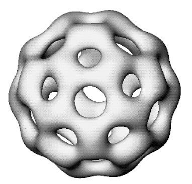
Given the explicit matrix (4.27) the real matrix $R(x)$, defined by (2.6), can be computed explicitly using MAPLE, and its determinant calculated to verify that it is non-zero. Using the formula (2.8) a MAPLE computation can generate an explicit expression for the topological charge density, but this is such a horrendous expression that it is not even efficient to use it to plot a topological charge density isosurface. In fact a much more efficient numerical scheme is to compute the determinant of the matrix $R(x)$ numerically and use a finite difference approximation to the derivatives in equation (2.8) to produce data for a plot. The results of this scheme are displayed in Fig. 1, where we present a topological charge density isosurface in $\hbox{\mybb R}^{3}\subset\hbox{\mybb R}^{4},$ obtained at zero Euclidean time $x_{4}=0.$ It can be seen that the topological charge density is localized around the ninety edges (and particularly the sixty vertices) of the truncated icosahedron of the buckyball, as predicted. As the only $x_{4}$ dependence of the matrix $R(x)$ is in the combination $|x|^{2}=x_{1}^{2}+x_{2}^{2}+x_{3}^{2}+x_{4}^{2},$ then isosurfaces for different Euclidean time slices are qualitatively similar, though the level set value needs to be reduced to correspond to the fact that the topological charge density decreases as $x_{4}^{2}$ increases.

Refer to caption
Figure 1: A topological charge density isosurface, in the Euclidean time slice $x_{4}=0,$ for the charge seventeen buckyball instanton.

For a suitable choice of scale, the holonomy of this instanton will provide a good approximation to the minimal energy charge seventeen Skyrmion. However, we have not investigated the energy of the resulting Skyrme field to determine the required scale since it is computationally expensive and a good approximation to this Skyrmion has already been obtained using a different approach [11].

5 Conclusion

The ADHM data has been obtained for an icosahedrally symmetric charge seventeen instanton with a buckyball structure. The existence of this instanton was predicted by studying Skyrmions, and this approach also predicts the existence of a whole range of fullerene instantons. However, it is not clear which fullerenes correspond to tractable ADHM data. There is evidence [3] that the minimal energy fullerene Skyrmion has icosahedral symmetry for charges in the sequence which begins $7,17,37,67,97,...$ As we have seen, icosahedral ADHM data is tractable for the first two charges in this sequence, so it may be tractable for others too.

Acknowledgements

I thank the EPSRC for an advanced fellowship.

References

  • [1] M.F. Atiyah, V.G. Drinfeld, N.J. Hitchin and Yu.I. Manin, Phys. Lett. A 65, 185 (1978).
  • [2] M.F. Atiyah and N.S. Manton, Phys. Lett. B 222, 438 (1989); Commun. Math. Phys. 153, 391 (1993).
  • [3] R.A. Battye, C.J. Houghton and P.M. Sutcliffe, J. Math. Phys. 44, 3543 (2003).
  • [4] R.A. Battye and P.M. Sutcliffe, Phys. Rev. Lett. 79, 363 (1997).
  • [5] R.A. Battye and P.M. Sutcliffe, Phys. Rev. Lett. 86, 3989 (2001); Rev. Math. Phys. 14, 29 (2002).
  • [6] E. Braaten, S. Townsend and L. Carson, Phys. Lett. B 235, 147 (1990).
  • [7] N.H. Christ, E.J. Weinberg and N.K. Stanton, Phys. Rev. D 18, 2013 (1978).
  • [8] E. Corrigan, D.B. Fairlie, P. Goddard and S. Templeton, Nucl. Phys. B 140, 31 (1978).
  • [9] H.S.M. Coxeter, Regular Complex Polytopes, Cambridge University Press (1974).
  • [10] N.J. Hitchin, N.S. Manton and M.K. Murray, Nonlinearity 8, 661 (1995).
  • [11] C.J. Houghton, N.S. Manton and P.M. Sutcliffe, Nucl. Phys. B 510, 507 (1998).
  • [12] C.J. Houghton and P.M. Sutcliffe, Commun. Math. Phys. 180, 343 (1996).
  • [13] C.J. Houghton and P.M. Sutcliffe, Nonlinearity 9, 385 (1996).
  • [14] R. Jackiw, C. Nohl and C. Rebbi, Phys. Rev. D 15, 1642 (1977).
  • [15] R.A. Leese and N.S. Manton, Nucl. Phys. A 572, 675 (1994).
  • [16] H. Osborn, Nucl. Phys. B 140, 45 (1978).
  • [17] M.A. Singer and P.M. Sutcliffe, Nonlinearity 12, 987 (1999).
  • [18] http://math.tntech.edu/rafal