Superfield covariant analysis of the divergence structure of noncommutative supersymmetric QED₄

Abstract

Commutative supersymmetric Yang-Mills is known to be renormalizable for ${\cal N}=1,2$, while finite for ${\cal N}=4$. However, in the noncommutative version of the model (NCSQED₄) the UV/IR mechanism gives rise to infrared divergences which may spoil the perturbative expansion. In this work we pursue the study of the consistency of NCSQED₄ by working systematically within the covariant superfield formulation. In the Landau gauge, it has already been shown for ${\cal N}=1$ that the gauge field two-point function is free of harmful UV/IR infrared singularities, in the one-loop approximation. Here we show that this result holds without restrictions on the number of allowed supersymmetries and for any arbitrary covariant gauge. We also investigate the divergence structure of the gauge field three-point function in the one-loop approximation. It is first proved that the cancellation of the leading UV/IR infrared divergences is a gauge invariant statement. Surprisingly, we have also found that there exist subleading harmful UV/IR infrared singularities whose cancellation only takes place in a particular covariant gauge. Thus, we conclude that these last mentioned singularities are in the gauge sector and, therefore, do not jeopardize the perturbative expansion and/or the renormalization of the theory.

I Introduction

During last years noncommutative (NC) field theories have been intensively studied. These theories emerged as the low energy limit of the open superstring in the presence of an external magnetic field ($B$-field) SW although nowadays they are interesting in their own right (for a review see Nekr ; Szabo ; Girotti11 ).

The most striking property of noncommutative field theories is undoubtly the UV/IR mechanism, through which the ultraviolet divergences (UV) are partly converted into infrared (IR) ones Minw ; Mat ; RR1 . These infrared divergences footnote1 may be so severe that the perturbative expansion of the theory becomes meaningless. Hence, the key point about the consistency of a noncommutative field theory is whether these divergences cancel out.

So far, only one four-dimensional noncommutative theory is known to be renormalizable, the Wess-Zumino model Girotti1 ; Buchbinder1 . In this case supersymmetry plays an essential role because it improves the ultraviolet behavior and, therefore, the UV/IR mechanism only generates mild UV/IR infrared divergences which do not spoil the renormalization program. In three space-time dimensions we are aware of at least two noncommutative renormalizable models: the supersymmetric $O(N)$ nonlinear sigma model sig and the $O(N)$ supersymmetric linear sigma model in the limit $N\rightarrow\infty$ linsm .

As for nonsupersymmetric gauge theories, the UV/IR mechanism breaks down the perturbative approach Mat ; RR1 ; Hay ; SJ ; Armoni ; Bonora ; FL ; Gur ; Nichol . Nevertheless, we can entertain the hope that noncommutative supersymmetric gauge theories are free from nonintegrable UV/IR infrared singularities and, furthermore, renormalizable. We are aware of the following results concerning noncommutative supersymmetric gauge field theories:

1) By working with the formalism of component fields Mat ; RR1 it has been shown that the dangerous UV/IR infrared divergences cancel in the one-loop contributions to the gauge field two and three-point functions. The two-point function turns out to contain quadratic and logarithmic UV divergences. Dimensional regularization takes care of the first ones while the last ones must be renormalized. As for the harmful infrared divergences originating through the UV/IR mechanism, they are only quadratic and cancel out within a supersymmetric multiplet. The three-point function is linearly UV divergent by power counting. However, this time, the leading UV divergences vanish by symmetric integration, while the IR poles originating from them cancel out among themselves.

2) By using the superfield formalism Bichl et al. bichl calculated, in the Landau gauge and in the absence of matter (${\cal N}=1$), the one-loop contributions to the two-point function of the gauge superfield. Only quadratic and logarithmic UV divergences are present and one deals with them as indicated in the previous paragraph. The quadratic infrared poles in the nonplanar part of the amplitude again cancel while the linear ones do not arise. The superfield formulation represents an improvement with respect to the component field formulation because supersymmetry is explicitly preserved at all stages of the calculation.

3) Zanon and collaborators Za1 ; Zanon used the background field method to evaluate the one-loop contributions to the field strength two-point functions in ${\cal N}=1,2$ supersymmetric Yang-Mills theories, where only logarithmic divergences were found. The three-point function was shown to vanish. For ${\cal N}=4$ they demonstrated that, up to one loop, there are no divergences at all.

This paper is dedicated to pursue further the study, within the superfield formulation, of the consistency of NCSQED₄ in an arbitrary covariant gauge. We analyze the divergence structure induced by the UV/IR mechanism in the two and three-point gauge field Green functions.

In Section 2 we establish our definitions and conventions and present the gauge invariant action describing the dynamics of NCSQED₄ in ${\cal N}=1$ superspace. Next, the gauge fixing and the Faddeev-Popov terms are found. Finally, we add chiral matter superfields and derive the Feynman rules of NCSQED₄ with extended supersymmetry.

We start, in Section 3, by reviewing the cancellation of the leading UV/IR infrared divergences in the one-loop corrections to the two-point function of the gauge superfieldbichl . A straightforward generalization shows that these results also hold for extended supersymmetry and/or when the theory is formulated in an arbitrary covariant gauge.

In Section 4 we compute the one-loop corrections to the three-point functions of the gauge superfield in an arbitrary covariant gauge. This is done for ${\cal N}=1,2,4$. From power counting follows that the amplitude is at the most quadratically divergent. As far as the planar part is concerned, dimensional regularization takes care of the quadratic UV divergences, the linear ones vanish by symmetric integration, while the logarithmic divergences are to be eliminated through renormalization. As for the nonplanar part, the UV/IR mechanism will be seen not to give rise to quadratic IR divergences but only to linear and logarithmic ones. Interestingly enough, the linear IR divergences arise from two different sources: a) integrals which, by power counting, are quadratically UV divergent but whose Moyal phase factor not only regularizes them but also lowers the degree of the IR divergence, b) integrals which are linearly UV divergent by power counting but regularized by the noncommutativity. The softening mechanism mentioned in a) also contributes IR logarithmic divergences, which, nevertheless, do not jeopardize the perturbative expansion.

The conclusions are contained in Section 5.

II The action and Feynman rules for NCSQED₄

II.1 The action

In ${\cal N}=1$ superspace NCSQED₄ is described by the nonpolynomial action SGRS ; footnoteSGRS

$$S_{V}\,=\,-\,\frac{1}{2g^{2}}\int d^{8}z\left(e^{-gV}*D^{\alpha}e^{gV}\right)*\overline{D}^{2}\left(e^{-gV}*D_{\alpha}e^{gV}\right)\,,$$ (1)

where $g$ is the coupling constant, $V$ is a real vector gauge superfield,

$$e^{gV}\,=\,\sum_{n\geq 0}\frac{1}{n!}\left(gV\right)^{*n}\,\equiv\,\sum_{n\geq 0}\frac{1}{n!}\,\left(\begin{array}[]{c}\underbrace{gV*gV*...gV}\\ n-times\end{array}\right)\,,$$ (2)

and $*$ denotes Moyal product of operators, i.e.,

$$\phi_{1}(x)\ast\phi_{2}(x)\,=\,\phi_{1}(x)\,exp\left(\frac{i}{2}\,\overleftarrow{\frac{\partial}{\partial x^{\mu}}}\,\Theta^{\mu\nu}\,\overrightarrow{\frac{\partial}{\partial x^{\nu}}}\right)\,\phi_{2}(x)$$

$$=\,\sum_{n=0}^{\infty}\,\left(\frac{i}{2}\right)^{n}\,\frac{1}{n!}\,\left[\partial_{\mu_{1}}\partial_{\mu_{2}}...\partial_{\mu_{n}}\,\phi_{1}(x)\right]\,\Theta^{\mu_{1}\nu_{1}}\Theta^{\mu_{2}\nu_{2}}...\Theta^{\mu_{n}\nu_{n}}\,\left[\partial_{\nu_{1}}\partial_{\nu_{2}}...\partial_{\nu_{n}}\,\phi_{2}(x)\right]\,.$$ (3)

Here, $\Theta^{\mu\nu}$ is the antisymmetric real constant matrix characterizing the noncommutativity of the underlying space-time. The expression

$$\int d^{4}x\varphi_{1}\left(x\right)*\cdots*\varphi_{n}\left(x\right)$$

$$=\,\int\left(\prod_{j=1}^{n}\frac{d^{4}k_{j}}{\left(2\pi\right)^{4}}\right)\left(2\pi\right)^{4}\delta\left(\sum_{1}^{n}k_{j}\right)e^{-i\sum_{i<j}k_{i}\wedge k_{j}}\varphi_{1}\left(k_{1}\right)\cdots\varphi_{n}\left(k_{n}\right)\,,$$ (4)

where

$$k_{i}\wedge k_{j}\,=\,\frac{1}{2}\,k^{\mu}_{i}\,k^{\nu}_{j}\,\Theta_{\mu\nu}\,,$$ (5)

will play a relevant role for determining the Feynman rules in the theory.

Under the group $U(1)$ of gauge transformations

$$U\,=\,e^{ig\Lambda}\,=\,\sum_{n\geq 0}\frac{1}{n!}\left(ig\Lambda\right)^{*n}\,,$$ (6)

with $\Lambda$ (${\bar{\Lambda}}=\Lambda^{\dagger}$) a chiral (antichiral) superfield, $V$ transforms as follows

$$e^{gV}\rightarrow e^{-ig{\Lambda}}*e^{gV}*e^{ig\overline{\Lambda}}\,,$$ (7)

thus leaving $S$ invariant.

In future, we shall be needing the expansion of $S$ in powers of $g$, up to the order $g^{3}$. To this end we first recall the identity Buchbinder2

$$e^{-gV}*D_{\alpha}e^{gV}\,$$ (8)

$$= \,gD_{\alpha}V-\frac{g^{2}}{2!}\left[V,D_{\alpha}V\right]_{*}+\frac{g^{3}}{3!}\left[V,\left[V,D_{\alpha}V\right]_{*}\right]_{*}-\frac{g^{4}}{4!}\left[V,\left[V,\left[V,D_{\alpha}V\right]_{*}\right]_{*}\right]_{*}$$

$$+\,\frac{g^{5}}{5!}\,\left[V,\left[V,\left[V,\left[V,D_{\alpha}V\right]_{*}\right]_{*}\right]_{*}\right]_{*}\,+\,\cdots\,.$$

Then, after by part integrations and by exploring the properties of the Moyal product footnote2 one obtains

$$S_{V}\,=\,S_{V}^{(0)}\,+\,g\,S_{V}^{(1)}\,+\,g^{2}\,S_{V}^{(2)}\,+\,g^{3}\,S_{V}^{(3)}\,+\,\cdots\,,$$ (9)

where

$$S_{V}^{(0)}\,=\,\frac{1}{2}\int d^{8}z\,V\,D^{\alpha}\overline{D}^{2}D_{\alpha}V\,,$$ (10)

$$S_{V}^{(1)}=\frac{1}{2}\int d^{8}z\,\overline{D}^{2}D^{\alpha}V*\left[V,D_{\alpha}V\right]_{*}\,,$$ (11)

$$S_{V}^{(2)}=-\,\int d^{8}z\left\{\frac{1}{8}\,\left[V,D^{\alpha}V\right]_{*}*\overline{D}^{2}\left[V,D_{\alpha}V\right]_{*}+\frac{1}{6}\,\overline{D}^{2}D^{\alpha}V*\left[V,\left[V,D_{\alpha}V\right]_{*}\right]_{*}\right\}\,,$$ (12)

$$S_{V}^{(3)} = \frac{1}{12}\int d^{8}z\left\{\frac{1}{2}\,\overline{D}^{2}D^{\alpha}V*\left[V,\left[V,\left[V,D_{\alpha}V\right]_{*}\right]_{*}\right]_{*}\right.$$ (13)

$$\left.+\left[V,\left[V,D^{\alpha}V\right]_{*}\right]_{*}*\overline{D}^{2}\left[V,D_{\alpha}V\right]_{*}\right\}\,.$$

As usual, gauge fixing is implemented by adding to the action $S_{V}$ the covariant term

$$S_{gf}\,=\,-\frac{a}{2}\int d^{8}zV\left\{D^{2},\overline{D}^{2}\right\}V\,,$$ (14)

where $a$ is a real number labeling the gauge. Clearly,

$$S_{V}^{(0)}\,+\,S_{gf}=\frac{1}{2}\int d^{8}z\,V\left(\Box+\left(1-a\right)\left\{D^{2},\overline{D}^{2}\right\}\right)V\,,$$ (15)

as seen from Eqs. (10) and (14).

For the covariant gauge $a$, the Faddeev-Popov determinant reads

$$\Delta^{-1}\left[V\right]\,=\,\int\mathcal{D}c\,\mathcal{D}c^{\prime}\,\mathcal{D}\overline{c}\,\mathcal{D}\overline{c}^{\prime}\,e^{-\,\int d^{8}z\,\left[c\left(z\right)+\overline{c}\left(z\right)\right]\,\delta V\left(z\right)}|_{\Lambda=c^{\prime}\,;\,\overline{\Lambda}=\overline{c}^{\prime}}\,.$$ (16)

Here $c,\overline{c}=c^{\dagger},c^{\prime},\overline{c}^{\prime}={c^{\prime}}^{\dagger}$ are the ghost fields while $\delta V$ denotes the change in $V$ provoked by an infinitesimal gauge transformation. One readily obtains from (7) that

$$\delta V\,=\,iL_{\frac{g}{2}V}\,\left[-\left(\Lambda+\overline{\Lambda}\right)+\left(\coth L_{\frac{g}{2}V}\right)\left[\overline{\Lambda}-\Lambda\right]\right]\,,$$ (17)

where

$$L_{A}\left[B\right]\equiv\left[A,B\right]_{*}\,.$$ (18)

After recalling the Laurent expansion of $\coth x$, around $x=0$, one arrives at

$$\delta V = iL_{\frac{g}{2}V}\left[-\left(\Lambda+\overline{\Lambda}\right)\right]$$ (19)

$$+ iL_{\frac{g}{2}V}\left[L_{\frac{g}{2}V}^{-1}\left[\overline{\Lambda}-\Lambda\right]+\frac{1}{3}L_{\frac{g}{2}V}\left[\overline{\Lambda}-\Lambda\right]\,+\,\cdots\right]$$

$$= i\left(\overline{\Lambda}-\Lambda\right)-\frac{ig}{2}\left[V,\Lambda+\overline{\Lambda}\right]_{*}+\frac{ig^{2}}{12}\left[V,\left[V,\overline{\Lambda}-\Lambda\right]_{*}\right]_{*}\,+\,\cdots\,.$$

Therefore, by going back with Eq. (19) into Eq. (16) one finds for the ghost action the following expression

$$S_{gh}\,=-\,S_{gh}^{(0)}\,+\,g\,S_{gh}^{(1)}\,+\,g^{2}\,S_{gh}^{(2)}\,+\,\cdots\,,$$ (20)

where

$$S_{gh}^{(0)}\,=\,-\,\int d^{8}z\left(c+\overline{c}\right)\left(\overline{c}^{\prime}-c^{\prime}\right)\,,$$ (21)

$$S_{gh}^{(1)}\,=\,\,\frac{1}{2}\int d^{8}z\,\left(c+\overline{c}\right)\left[V,c^{\prime}+\overline{c}^{\prime}\right]_{*}\,,$$ (22)

$$S_{gh}^{(2)}\,=\,-\frac{1}{12}\int d^{8}z\,\left(c+\overline{c}\right)\left[V,\left[V,\overline{c}^{\prime}-c^{\prime}\right]_{*}\right]_{*}\,.$$ (23)

In addition to the real vector superfield we introduce now a chiral matter superfield $\Phi$ in the adjoint representation. This enables us to construct a theory in which the ${\cal N}=2$ supersymmetry is realized. The generalization to ${\cal N}=4$ is straightforward and will be done afterwards. The corresponding action describing the free matter superfield as well as its interaction with the gauge superfield reads

$$S_{m}\,=\,\int d^{8}z\overline{\Phi}*e^{-gV}*\Phi*e^{gV}\,,$$ (24)

whose invariance under supergauge transformations follows from (7) together with

$$\Phi\rightarrow\Phi^{\prime}\,=\,e^{ig{\bar{\Lambda}}}*\Phi*e^{ig{\Lambda}}\,,\,\,\,\,\,\,\,\,\,\,\,\,{\bar{\Phi}}\rightarrow{\bar{\Phi}}^{\prime}\,=\,e^{-ig{\bar{\Lambda}}}*{\bar{\Phi}}*e^{-ig{\Lambda}}\,.$$ (25)

The first four terms of the expansion of $S_{m}$ as a power series of $g$,

$$S_{m}\,=\,S_{m}^{(0)}\,+\,g\,S_{m}^{(1)}\,+\,g^{2}\,S_{m}^{(2)}\,+\,g^{3}\,S_{m}^{(3)}\,+\,\cdots\,,$$ (26)

are found to be

$$S_{m}^{(0)}\,=\,\int\,d^{8}z\,\overline{\Phi}{\Phi}\,,$$ (27)

$$S_{m}^{(1)}\,=\,-\int d^{8}z\,\overline{\Phi}*\left[V,\Phi\right]_{*}\,,$$ (28)

$$S_{m}^{(2)}\,=\,\frac{1}{2}\int d^{8}z\,\overline{\Phi}*\left[V,\left[V,\Phi\right]_{*}\right]_{*}\,,$$ (29)

$$S_{m}^{(3)}\,=\,-\frac{1}{6}\int d^{8}z\,\overline{\Phi}*\left[V,\left[V,\left[V,\Phi\right]_{*}\right]_{*}\right]_{*}\,.$$ (30)

II.2 Feynman rules

From the quadratic part of the action $S_{V}^{(0)}+S_{gf}+S_{gh}^{(0)}+S_{m}^{(0)}$ one obtains, through standard manipulations, the free propagators

$$\Delta_{VV}(z_{1}-z_{2})\,=\,\frac{i}{\Box}\,\left[1\,+\,(1-a)\,\frac{1}{\Box}\,\{D_{1}^{2},{\overline{D}}_{1}^{2}\}\right]\,\delta^{8}(z_{1}-z_{2})\,,$$ (31a)

$$\Delta_{{\overline{c}}c^{\prime}}(z_{1}-z_{2})\,=\,-\,\frac{i}{\Box}\,D_{1}^{2}\,\overline{D}_{2}^{2}\,\delta^{8}(z_{1}-z_{2}),$$ (31b)

$$\Delta_{c{\overline{c}}^{\prime}}(z_{1}-z_{2})\,=\,\frac{i}{\Box}\,{\overline{D}}_{1}^{2}\,{D}_{2}^{2}\,\delta^{8}(z_{1}-z_{2})\,,$$ (31c)

$$\Delta_{\Phi\overline{\Phi}}(z_{1}-z_{2})\,=\,-\,\frac{i}{\Box}\,{\overline{D}}_{1}^{2}\,{D}_{2}^{2}\,\delta^{8}(z_{1}-z_{2})\,,$$ (31d)

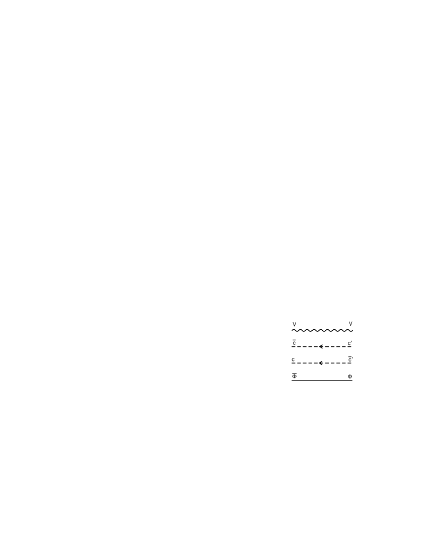
Figure 1: Free propagators. The arrow indicates the flux of ghost charge.

corresponding to the gauge, ghosts and matter superfields, respectively. They are depicted in Fig. 1.

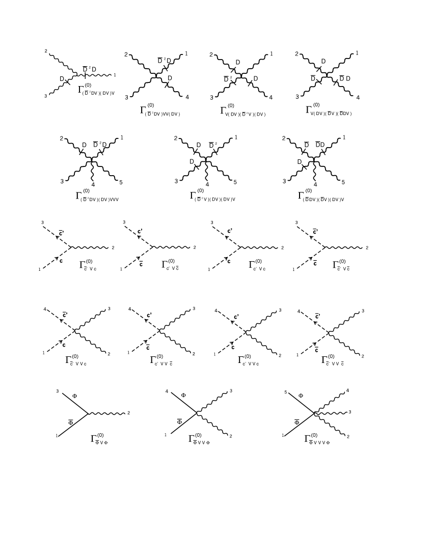
Figure 2: Elementary vertices.

On the other hand, the interacting part of the total action together with Eq. (II.1) enable us to find the elementary vertices $\Gamma^{(0)}$ in the theory. They are displayed in Fig. 2. In an obvious notation

$$\Gamma_{(\overline{D}^{2}DV)(DV)V}^{(0)}(k_{1},k_{2},k_{3})\,=\,g\,{\cal V}_{3}(k_{1},k_{2},k_{3})\,,$$ (32)

$$\Gamma_{(\overline{D}^{2}DV)(DV)VV}^{(0)}(k_{1},k_{2},k_{3},k_{4})\,=\,-\,\frac{ig^{2}}{12}\,{\cal V}^{(1)}_{4}(k_{1},k_{2},k_{3},k_{4})\,,$$ (33a)

$$\Gamma_{V(DV)(\overline{D}V)({\overline{D}}DV)}^{(0)}(k_{1},k_{2},k_{3},k_{4})\,=\,ig^{2}\,{\cal V}^{(2)}_{4}(k_{1},k_{2},k_{3},k_{4})\,,$$ (33b)

$$\Gamma_{V(DV)(\overline{D}^{2}V)(DV)}^{(0)}(k_{1},k_{2},k_{3},k_{4})\,=\,ig^{2}\,{\cal V}^{(2)}_{4}(k_{1},k_{2},k_{3},k_{4})\,,$$ (33c)

$$\Gamma_{(\overline{D}^{2}DV)(DV)VVV}^{(0)}(k_{1},k_{2},k_{3},k_{4},k_{5})\,=\,-\,\frac{g^{3}}{36}\,{\cal V}_{5}^{(1)}(k_{1},k_{2},k_{3},k_{4},k_{5})\,,$$ (34a)

$$\Gamma_{VV(DV)(\overline{D}DV)({\overline{D}}V)}^{(0)}(k_{1},k_{2},k_{3},k_{4},k_{5})\,=\,-\,\frac{2g^{3}}{3}\,{\cal V}_{5}^{(2)}(k_{1},k_{2},k_{3},k_{4},k_{5})\,,$$ (34b)

$$\Gamma_{VV(DV)(\overline{D}^{2}V)(DV)}^{(0)}(k_{1},k_{2},k_{3},k_{4},k_{5})\,=\,\frac{ig^{3}}{12}\,{\cal V}_{5}^{(3)}(k_{1},k_{2},k_{3},k_{4},k_{5})\,,$$ (34c)

$$\Gamma_{{\overline{c}}^{\prime}Vc}^{(0)}(k_{1},k_{2},k_{3})\,=\,g\,{\cal V}_{3}(k_{1},k_{2},k_{3})\,,$$ (35a)

$$\Gamma_{{c}^{\prime}V{\overline{c}}}^{(0)}(k_{1},k_{2},k_{3})\,=\,g\,{\cal V}_{3}(k_{1},k_{2},k_{3})\,,$$ (35b)

$$\Gamma_{{c}^{\prime}Vc}^{(0)}(k_{1},k_{2},k_{3})\,=\,-\,g\,{\cal V}_{3}(k_{1},k_{2},k_{3})\,,$$ (35c)

$$\Gamma_{{\overline{c}}^{\prime}V{\overline{c}}}^{(0)}(k_{1},k_{2},k_{3})\,=\,-\,g\,{\cal V}_{3}(k_{1},k_{2},k_{3})\,\,,$$ (35d)

$$\Gamma_{\overline{c}^{\prime}VVc}^{(0)}(k_{1},k_{2},k_{3},k_{4})\,=\,-\,\frac{ig^{2}}{6}\,{\cal V}^{(1)}_{4}(k_{1},k_{2},k_{3},k_{4})\,,$$ (36a)

$$\Gamma_{c^{\prime}VV{\overline{c}}}^{(0)}(k_{1},k_{2},k_{3},k_{4})\,=\,\frac{ig^{2}}{6}\,{\cal V}^{(1)}_{4}(k_{1},k_{2},k_{3},k_{4})\,,$$ (36b)

$$\Gamma_{c^{\prime}VVc}^{(0)}(k_{1},k_{2},k_{3},k_{4})\,=\,\frac{ig^{2}}{6}\,{\cal V}^{(1)}_{4}(k_{1},k_{2},k_{3},k_{4})\,,$$ (36c)

$$\Gamma_{\overline{c}^{\prime}VV{\overline{c}}}^{(0)}(k_{1},k_{2},k_{3},k_{4})\,=\,-\,\frac{ig^{2}}{6}\,{\cal V}^{(1)}_{4}(k_{1},k_{2},k_{3},k_{4})\,,\,$$ (36d)

$$\Gamma_{\overline{\Phi}V\Phi}^{(0)}(k_{1},k_{2},k_{3})\,=\,2\,g\,{\cal V}_{3}(k_{1},k_{2},k_{3})\,,$$ (37a)

$$\Gamma_{\overline{\Phi}VV\Phi}^{(0)}(k_{1},k_{2},k_{3},k_{4})\,=\,i\,g^{2}\,{\cal V}_{4}^{(1)}(k_{1},k_{2},k_{3},k_{4})\,,$$ (37b)

$$\Gamma_{\overline{\Phi}VVV\Phi}^{(0)}(k_{1},k_{2},k_{3},k_{4},k_{5})\,=\,-\,\frac{g^{3}}{9}\,{\cal V}_{5}^{(1)}(k_{1},k_{2},k_{3},k_{4},k_{5})\,.$$ (37c)

Here,

$${\cal V}_{3}(k_{1},k_{2},k_{3})\,=\,\sin(k_{1}\wedge k_{2})\,,$$ (38a)

$${\cal V}^{(1)}_{4}(k_{1},k_{2},k_{3},k_{4})\,=\,\cos(k_{2}\wedge k_{3})\,\cos(k_{1}\wedge k_{4})\,-\,\cos(k_{1}\wedge k_{2}\,-\,k_{3}\wedge k_{4})\,,$$ (38b)

$${\cal V}^{(2)}_{4}(k_{1},k_{2},k_{3},k_{4})\,=\,\frac{1}{2}\,\left[\sin(k_{1}\wedge k_{2})\sin(k_{3}\wedge k_{4})-\sin(k_{1}\wedge k_{4})\sin(k_{2}\wedge k_{3})\right]\,,$$ (38c)

$${\cal V}^{(1)}_{5}(k_{1},k_{2},k_{3},k_{4},k_{5})\,=\,\left[2\,\cos(k_{4}\wedge k_{5})\,\cos(k_{3}\wedge k_{4}\,+\,k_{3}\wedge k_{5})\right.$$

$${\phantom{abc}}+\left.\,\cos(-k_{3}\wedge k_{4}\,+\,k_{4}\wedge k_{5}\,+\,k_{3}\wedge k_{5})\,\right]\,\sin(k_{1}\wedge k_{2})$$

$${\phantom{abc}}+\,3\,\left[\cos(-k_{2}\wedge k_{3}\,+\,k_{2}\wedge k_{5}\,+\,k_{3}\wedge k_{5})\,\sin(k_{1}\wedge k_{4})\right.$$

$${\phantom{abc}}+\left.\,\cos(-k_{2}\wedge k_{4}\,+\,k_{4}\wedge k_{5}\,+\,k_{2}\wedge k_{5})\,\sin(k_{1}\wedge k_{3})\right.$$

$${\phantom{abc}}+\left.\,\cos(-k_{2}\wedge k_{4}\,-\,k_{3}\wedge k_{4}\,+\,k_{2}\wedge k_{3})\,\sin(k_{1}\wedge k_{5})\right]\,,\,$$ (38d)

$${\cal V}^{(2)}_{5}(k_{1},k_{2},k_{3},k_{4},k_{5})\,=\,2\sin(p_{1}\wedge p_{3})\sin(p_{2}\wedge p_{3})\cos(p_{1}\wedge p_{2})$$

$${\phantom{abc}}+\sin(p_{1}\wedge p_{2})\,\left[\sin(p_{2}\wedge p_{3}-p_{1}\wedge p_{3})\right]\,,$$ (38e)

$${\cal V}^{(3)}_{5}(k_{1},k_{2},k_{3},k_{4},k_{5})\,=\,2\,i\,\sin(p_{1}\wedge p_{2})\cos(p_{2}\wedge p_{4})\cos(p_{3}\wedge p_{5})$$

$${\phantom{abc}}+\,\exp(-ip_{1}\wedge p_{2})\,\cos(p_{3}\wedge p_{4}+p_{3}\wedge p_{5}+p_{4}\wedge p_{5})$$

$${\phantom{abc}}+\,\exp(-ip_{1}\wedge p_{4})\,\cos(p_{3}\wedge p_{2}+p_{3}\wedge p_{5}+p_{2}\wedge p_{5})$$

$${\phantom{abc}}-\,\exp(-ip_{1}\wedge p_{3})\,\cos(p_{2}\wedge p_{5}+p_{2}\wedge p_{4}-p_{4}\wedge p_{5})$$

$${\phantom{abc}}-\,\exp(-ip_{1}\wedge p_{5})\,\cos(p_{2}\wedge p_{3}+p_{2}\wedge p_{4}-p_{3}\wedge p_{4})\,,$$ (38f)

the momenta are taken positive when entering the vertex and momentum conservation holds in all vertices.

We close this Section by pointing out that the superficial degree of divergence of a generic Feynman graph ${\cal G}$ is given by SGRS

$$d[{\cal G}]\,=\,2\,-\,E_{c}\,,$$ (39)

where $E_{c}$ is the number of external chiral lines. As known, in a noncommutative quantum field theory, a generic Feynman graph ${\cal G}$ will decompose into planar and nonplanar parts. The superficial degree of UV divergence of the planar part is measured by $d[{\cal G}]$. The nonplanar part is free of UV divergences but afflicted by IR singularities generated through the UV/IR mechanism Minw ; footnote1 , in this last connection $d[{\cal G}]$ also gives the highest possible degree of the IR divergences.

III One loop-contributions to the vector gauge superfield two-point function $\Gamma^{(1)}_{VV}$.

The cancellation of the harmful UV/IR infrared divergences in $\Gamma^{(1)}_{VV}$ was already proved in bichl for ${\cal N}=1$ and by working in the Landau gauge. Here, the proof is generalized by showing that the just mentioned cancellation takes place for an arbitrary covariant gauge and extended supersymmetry.

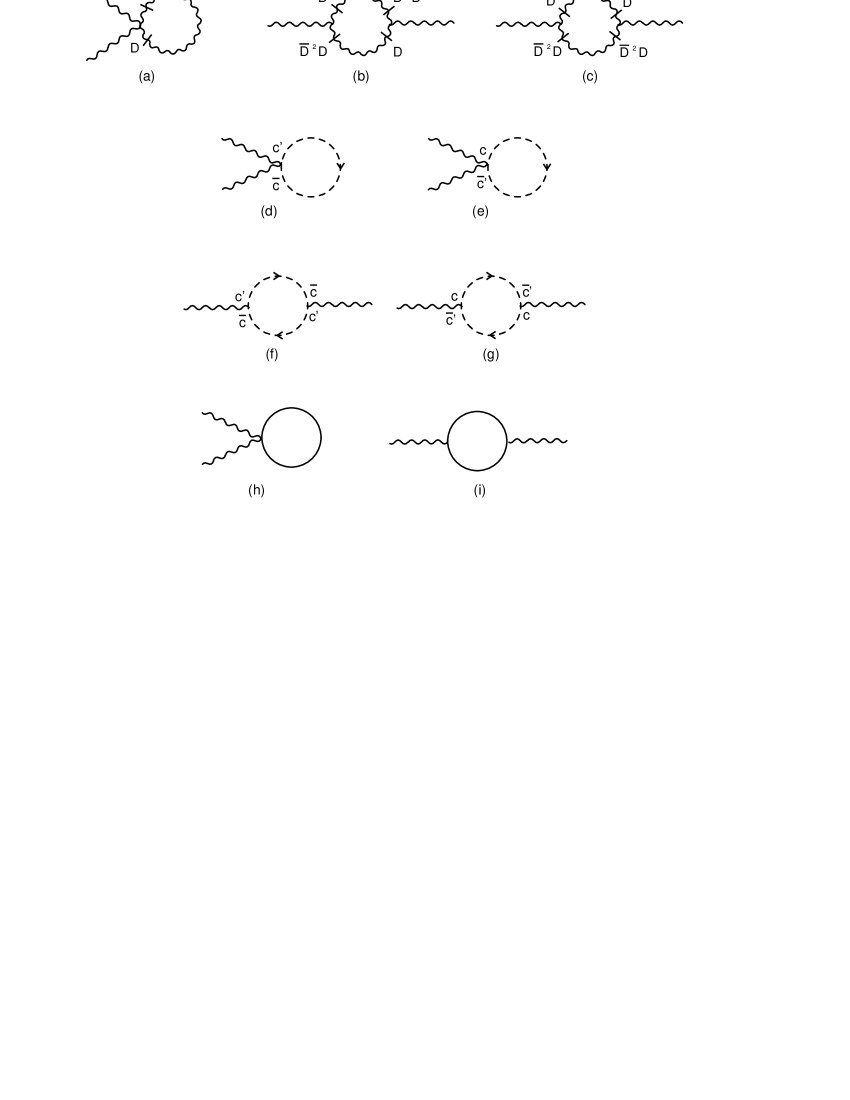
Figure 3: Diagrams contributing to $\Gamma^{(1)}_{VV}$.

Let us first concentrate on the graphs involving either a $V$ tadpole or a $V$ loop (see Fig. 3). Since there are no external chiral lines, $d[{\cal G}]=2$. Now, only those graphs with all $D$ factors in the internal lines may exhibit quadratic UV divergences. Diagrams with a factor $D$ and/or a ${\overline{D}}$ on the external lines can at the most be linearly divergent. Any other combination of $D$’s on the external lines corresponds to contributions which are logarithmically divergent or finite. These follows from the $D$-algebra alone SGRS . However, one is to take into account also the noncommutativity, which gives origin to a trigonometric factor that modifies the Feynman integrands. The combination of these two ingredients rules out, for the diagrams under analysis, the UV and UV/IR infrared linearly divergent terms. Hence, in this case, only quadratic divergences may jeopardize the consistency of the theory. They are contained in graphs (a), (b) and (c) in Fig. 3.

From the Feynman rules derived in Section 2, we found that the contribution ${\Gamma}_{VV;3{\rm a}}^{(1)}$ arising from the $V$ tadpole diagram is given by

$${\Gamma}_{VV;3{\rm a}}^{(1)}(p)$$ (40)

$$= -\frac{g^{2}}{6}\int\frac{d^{4}k}{\left(2\pi\right)^{4}}d^{4}\theta_{1}d^{4}\theta_{2}\mathcal{V}^{(1)}_{4}\left(-k,p,-p,k\right)\frac{\delta_{12}}{k^{2}}\left(\overline{D}_{1}^{2}D_{1}^{\alpha}D_{2\alpha}\delta_{12}\right)V\left(p,\theta_{1}\right)V\left(-p,\theta_{2}\right).$$

Here, a factor $2$ coming from the permutation of the external legs has already been taken into account. Moreover, we note that the term proportional to $(1-a)$ in the right hand side of (31a) does not contribute.

From (38b) one finds that

$$\mathcal{V}_{4}^{(1)}\left(-k,p,-p,k\right)\,=\,2\sin^{2}(k\wedge p)\,.$$ (41)

After $D$-algebra manipulations, one ends up with

$$\Gamma_{VV;3{\rm a}}^{(1)}(p)\,=\,\frac{2}{3}\,g^{2}\,A\,,$$ (42)

where

$$A\,\equiv\,\int\frac{d^{4}k}{\left(2\pi\right)^{4}}\,d^{4}\theta\,\frac{\sin^{2}(k\wedge p)}{k^{2}}\,V\left(p,\theta\right)\,V\left(-p,\theta\right)\,.$$ (43)

The planar part of $A$ only contains quadratic UV divergences, while the nonplanar one only develops quadratic IR infrared singularities.

The amplitudes associated with diagrams (b) and (c) of Fig. 3 are, respectively,

$$\Gamma_{VV;3{\rm b}}^{(1)}(p)\, = \,2\,\times\,\frac{1}{2}\,g^{2}\,\int\frac{d^{4}k}{(2\pi)^{4}}\,d^{4}\theta_{1}\,d^{4}\theta_{2}\,{\cal V}_{3}(k-p,p,-k)\,{\cal V}_{3}(k,-p,-k+p)\,$$ (44)

$$\times \left[-\,\frac{1}{k^{2}(k+p)^{2}}\right]D^{\alpha}_{1}\,{\overline{D}}^{2}_{2}\,D^{\beta}_{2}\,\delta_{12}\,D_{2\beta}\,{\overline{D}}^{2}_{1}\,D_{1\alpha}\,\delta_{12}\,V(p,\theta_{1})\,V(-p,\theta_{2})\,,$$

$$\Gamma_{VV;3{\rm c}}^{(1)}(p)\, = \,2\,\times\,\frac{1}{2}\,g^{2}\,\int\frac{d^{4}k}{(2\pi)^{4}}\,d^{4}\theta_{1}\,d^{4}\theta_{2}\,{\cal V}_{3}(k-p,p,-k)\,{\cal V}_{3}(-k+p,-p,k)\,$$ (45)

$$\times \left[-\,\frac{1}{k^{2}(k+p)^{2}}\right]D^{\alpha}_{1}\,D^{\beta}_{2}\,\delta_{12}\,{\overline{D}}^{2}_{2}\,D_{2\beta}\,{\overline{D}}^{2}_{1}\,D_{1\alpha}\,\delta_{12}\,V(p,\theta_{1})\,V(-p,\theta_{2})\,,$$

where the $1/2$ comes from the second order of the perturbative expansion. After standard rearrangements one gets

$$\Gamma_{VV;3{\rm b}}^{(1)}(p)\, = \,g^{2}\,\int\frac{d^{4}k}{(2\pi)^{4}}\,d^{4}\theta\,{\cal V}_{3}(k-p,p,-k)\,{\cal V}_{3}(k,-p,-k+p)\,\left[-\,\frac{1}{k^{2}(k+p)^{2}}\right]$$ (46)

$$\times \,\left[-2\,V(p,\theta)\,\left(k^{2}\,+\,{\not\!k}_{\alpha{\dot{\alpha}}}\,{\overline{D}}^{{\dot{\alpha}}}\,D^{\alpha}\right)V(-p,\theta)\right]\,+\,LDT\,,$$

$$\Gamma_{VV;3{\rm c}}^{(1)}(p)\, = \,g^{2}\,\int\frac{d^{4}k}{(2\pi)^{4}}\,d^{4}\theta\,{\cal V}_{3}(k-p,p,-k)\,{\cal V}_{3}(-k+p,-p,k)\,\left[-\,\frac{1}{k^{2}(k+p)^{2}}\right]$$ (47)

$$\times \,\left[-2\,k^{2}\,V(p,\theta)\,V(-p,\theta)\right]\,.$$

Here, $LDT$ is short for all terms which are at the most logarithmically divergent. Furthermore, from Eq. (38a)

$${\cal V}_{3}(k-p,p,-k)\,{\cal V}_{3}(k,-p,-k+p)$$ (48)

$$= \,-\,{\cal V}_{3}(k-p,p,-k)\,{\cal V}_{3}(-k+p,-p,k)\,=\,-\,\sin^{2}(k\wedge p)\,.$$

As a result, the terms proportional to $k^{2}$, in the second brackets in the right hand sides of Eqs. (46) and (47), drop out in the sum $\Gamma_{VV;3{\rm b}}^{(1)}(p)\,+\,\Gamma_{VV;3{\rm c}}^{(1)}(p)$. On the other hand, the term proportional to ${\not\!k}_{\alpha{\dot{\alpha}}}$ in Eq. (46) survives. From power counting follows that such term might give rise to (dangerous) linear divergences. To see whether this really happens, we start by expanding

$$-\,\frac{1}{k^{2}(k+p)^{2}}\,,$$ (49)

around $p=0$. It is then obvious that the would be linearly divergent integral

$$\int\frac{d^{4}k}{(2\pi)^{4}}\,{\not\!k}_{\alpha{\dot{\alpha}}}\,\frac{1}{k^{4}}\,\sin^{2}(k\wedge p)\,,$$ (50)

vanishes by symmetric integration. As stated above, the even parity of the trigonometric factor in Eq. (43), eliminates the linear UV divergences and also the linear UV/IR infrared divergences. To summarize:

$$\Gamma_{VV;3{\rm b}}^{(1)}(p)\,+\,\Gamma_{VV;3{\rm c}}^{(1)}(p)\,=\,LDT\,.$$ (51)

We turn next into computing the ghost contributions to $\Gamma^{(1)}_{VV}$. A direct consequence of the $D$-algebra is that graphs containing any of the vertices $\Gamma^{(0)}_{c^{\prime}Vc}$, $\Gamma^{(0)}_{{\overline{c}}^{\prime}V{\overline{c}}}$, $\Gamma^{(0)}_{c^{\prime}VVc}$, or $\Gamma^{(0)}_{{\overline{c}}^{\prime}VV{\overline{c}}}$, depicted in Fig. 2, only contribute $LDT$. We shall therefore concentrate on the diagrams which might provide quadratic and/or linear divergent contributions to $\Gamma^{(1)}_{VV}$. These are the graphs (d) and (e) of Fig. 3.

The calculation of the tadpole contributions (graphs (d) and (e) in Fig. 3) $\Gamma_{VV;3{\rm d}}^{\left(1\right)}\left(p\right)$ is straightforward and yields

$$\Gamma_{VV;3{\rm d}}^{\left(1\right)}\left(p\right)=+\frac{g^{2}}{3}\int\frac{d^{4}k}{\left(2\pi\right)^{4}}\,d^{4}\theta\,\frac{\mathcal{V}_{4}^{(1)}\left(k,p,-p,-k\right)}{k^{2}}\,V\left(p,\theta\right)\,V\left(-p,\theta\right)\,.$$ (52)

The same expression arises for $\Gamma_{VV;3{\rm e}}^{\left(1\right)}\left(p\right)$. Then, after using (41), one obtains

$$\Gamma_{VV;3{\rm d}}^{\left(1\right)}\left(p\right)\,+\,\Gamma_{VV;3{\rm e}}^{\left(1\right)}\left(p\right)\,=\,\frac{4}{3}\,g^{2}\,A\,.$$ (53)

The evaluation of the ghost loop contributions (graphs (f) and (g) in Fig. 3) is a little bit more involved. By applying the Feynman rules we obtain

$$\Gamma_{VV;3{\rm f}}^{\left(1\right)}\left(p\right)\,=\,\left(-1\right)\times 2\times\frac{1}{2!}\times g^{2}$$ (54)

$$\times \int\frac{d^{4}k}{\left(2\pi\right)^{4}}d^{4}\theta_{1}d^{4}\theta_{2}\,\mathcal{V}_{3}\left(k,p,-p-k\right){\cal V}_{3}\left(p+k,-p,-k\right)\,V\left(p,\theta_{1}\right)\,V\left(-p,\theta_{2}\right)$$

$$\times \left[i\,\left(\overline{D}^{2}D^{2}\right)\frac{\delta_{12}}{\left(k+p\right)^{2}}\right]\left[i\,\left(D^{2}\overline{D}^{2}\right)\frac{\delta_{12}}{k^{2}}\right]\,,$$

where the $-1$ arises from the ghost loop and

$$\mathcal{V}_{3}\left(k,p,-p-k\right)\,{\cal V}_{3}\left(p+k,-p,-k\right)\,=\,-\,\sin^{2}(k\wedge p)\,.$$ (55)

It turns out that $\Gamma_{VV;3{\rm f}}^{\left(1\right)}\,=\,\Gamma_{VV;3{\rm g}}^{\left(1\right)}$. Therefore,

$$\Gamma_{VV;3{\rm f}}^{\left(1\right)}\left(p\right)\,+\,\Gamma_{VV;3{\rm g}}^{\left(1\right)}\left(p\right)\,=\,-\,2\,g^{2}\,A\,+\,LDT\,.$$ (56)

We stress, once again, that the would be linear divergences in Eqs. (52) and (56) are wiped out by symmetric integration.

From Eqs. (42), (51), (53), and (56) follows that the quadratic UV and the UV/IR infrared divergences do not show up for ${\cal N}=1$, in any arbitrary covariant gauge.

We shall next investigate the consequences of adding one matter superfield to get the ${\cal N}=2$ theory. The amplitudes associated with the graphs (h) and (i) in Fig. 3 are

$$\Gamma_{VV;3{\rm h}}^{(1)}(p)=2\,(ig^{2})\,\int\frac{d^{4}k}{\left(2\pi\right)^{4}}d^{4}\theta\,\mathcal{V}_{4}\left(k,p,-p,-k\right)\,\left[i\,\left(\overline{D}^{2}D^{2}\right)\frac{\delta_{11}}{k^{2}}\right]\,V\left(-p,\theta\right)V\left(p,\theta\right)\,$$ (57)

and

$$\Gamma_{VV;3{\rm i}}^{(1)}(p)\, = \,(-\,2\,g)^{2}\,\int\frac{d^{4}k}{\left(2\pi\right)^{4}}d^{4}\theta_{1}d^{4}\theta_{2}\,\mathcal{V}_{3}\,\left(-p-k,p,k\right)\,\mathcal{V}_{3}\left(-k,-p,p+k\right)$$ (58)

$$\times \left[i\,\left(\overline{D}^{2}D^{2}\right)\frac{\delta_{12}}{\left(k+p\right)^{2}}\right]\left[i\,\left(D^{2}\overline{D}^{2}\right)\frac{\delta_{12}}{k^{2}}\right]\,V\left(p,\theta_{1}\right)\,V\left(-p,\theta_{2}\right)\,.$$

By taking into account Eqs. (41) and (55) one obtains

$$\Gamma_{VV;3{\rm h}}^{(1)}(p)\,=\,-\,4\,g^{2}\,A\,,$$ (59)

and

$$\Gamma_{VV;3{\rm i}}^{(1)}(p)\,=\,4\,g^{2}\,A\,+\,LDT\,.$$ (60)

Therefore, up to LDT, $\Gamma_{VV;3{\rm h}}^{(1)}\,+\,\Gamma_{VV;3{\rm i}}^{(1)}\,=\,0$ implying in the absence of quadratic UV and UV/IR infrared divergences in the matter sector and, therefore, in the full ${\cal N}=2$ NCSQED₄. The validity of this conclusion for ${\cal N}=4$ is clear. Furthermore the UV logarithmic divergences are also absent in ${\cal N}=4$ in agreement with Za1 ; Zanon .

IV One loop-contributions to the vector gauge superfield three-point function ${\Gamma}_{VVV}^{(1)}$

We present in this Section the computation of the one-loop corrections to the V gauge field three-point function in the covariant superfield formalism. The divergence structure of the superfield formulation is, as we shall see, substantially different of that encountered by Matusis et al. Mat in the component formulation. As for the background field three-point function computed in Za1 ; Zanon our results play an essential role when considering insertions in higher order corrections such as the one indicated in Fig. 4.

The one-loop diagrams contributing to the the three-point gauge field function $\Gamma^{(1)}_{VVV}$ contain, generally speaking, a planar and a nonplanar part. The planar parts will exhibit, at the most, quadratic UV divergences, in agreement with Eq. (39). These divergences will be eliminated by dimensional regularization. The linear UV divergences are always wiped out by symmetric integration. Renormalization takes care of the logarithmic UV divergences. As for the nonplanar parts the situation will be seen to be more involved. Due to the peculiar structure of the Moyal trigonometric factors, quadratic UV divergences do not translate into quadratic UV/IR infrared singularities, but rather into linear and logarithmic ones. Hereafter, we shall refer to this effect as to the softening mechanism of divergences. There are, of course, linear infrared divergences arising from the would be linear UV divergences through the UV/IR mechanism. Finally, the logarithmic UV/IR infrared singularities are harmless and shall be left out of consideration.

Before facing the problem of selecting the diagrams of interest, we found appropriate to exemplify how the softening mechanism of divergences works. To this end, let us first consider the integral

$$I^{\mu}(p_{1},p_{2},p_{3})\,\equiv\,-\frac{1}{4}\,\int\,\frac{d^{4}k}{(2\pi)^{4}}\,\left[\sin\left(2k\wedge p_{1}\right)\,+\,\sin\left(2k\wedge p_{2}\right)\,+\,\sin\left(2k\wedge p_{3}\right)\right]\,\frac{k^{\mu}}{k^{4}}\,.$$ (61)

An straightforward computation yields

$$I^{\mu}\,(p_{1},p_{2},p_{3})\,\xrightarrow[p_{1},p_{2},p_{3}\rightarrow 0]{}\,\frac{i}{2\pi^{2}}\,\Theta^{\mu\nu}\,\left(\frac{p_{1\nu}}{p_{1}\circ p_{1}}\,+\,\frac{p_{2\nu}}{p_{2}\circ p_{2}}\,+\,\frac{p_{3\nu}}{p_{3}\circ p_{3}}\right)\,,$$ (62)

where

$$p\circ p\,\equiv\,p^{\mu}\,\left(\Theta^{2}\right)_{\mu\nu}\,p^{\nu}\,.$$ (63)

From observation follows that $I^{\mu}\,(p_{1},p_{2},p_{3})$ exhibits a linear infrared divergence. However, a nonplanar Feynman diagram whose corresponding amplitude is proportional to

$$\sin(p_{1}\wedge p_{2})\,I^{\mu}\,(p_{1},p_{2},p_{3})\,,$$ (64)

will be finite if only one of the momenta goes to zero and vanishing if one lets all momenta to zero simultaneously. On the other hand, an amplitude proportional to

$$\cos(p_{1}\wedge p_{2})\,I^{\mu}\,(p_{1},p_{2},p_{3})\,,$$ (65)

will certainly have a linear divergence at $p_{i}\rightarrow 0$. Needless to say, the conversion of quadratic UV divergences into linear UV/IR infrared divergences is also possible through this softening mechanism of divergences.

We turn back into our main line of development and look for the diagrams which can make IR harmful contributions to $\Gamma^{(1)}_{VVV}$. To this end, one is to take into consideration the $D$-algebra, the parity of the Feynman integrands, and the softening mechanism described above.

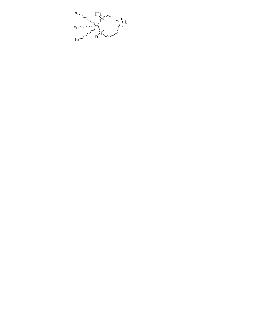
Figure 5: Tadpole contribution to $\Gamma^{(1)}_{VVV}$.

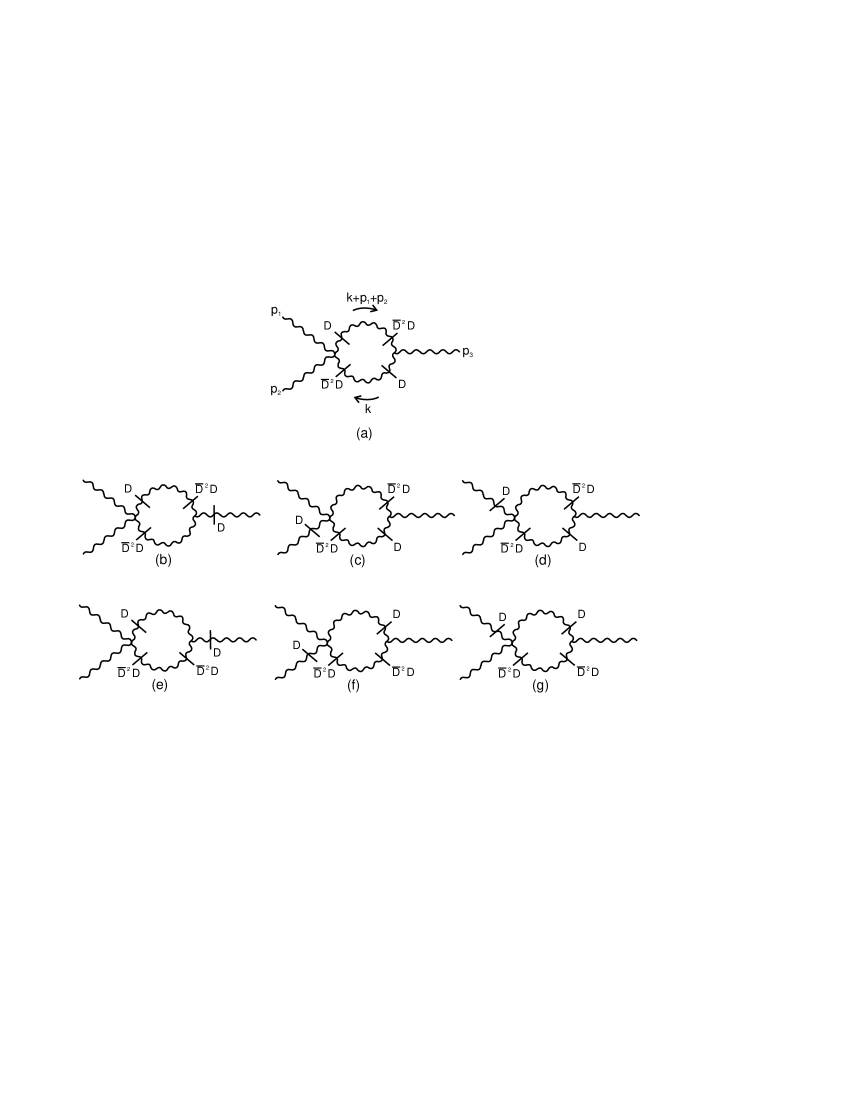
Figure 6: Contributions to $\Gamma^{(1)}_{VVV}$ involving the vertex $\Gamma_{(\overline{D}^{2}DV)(DV)VV}^{(0)}$.

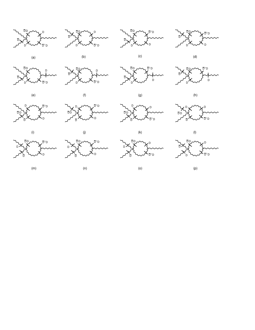
Figure 7: Contributions to $\Gamma^{(1)}_{VVV}$ involving the vertex $\Gamma_{V(DV)(\overline{D}V)({\overline{D}}DV)}^{(0)}$.

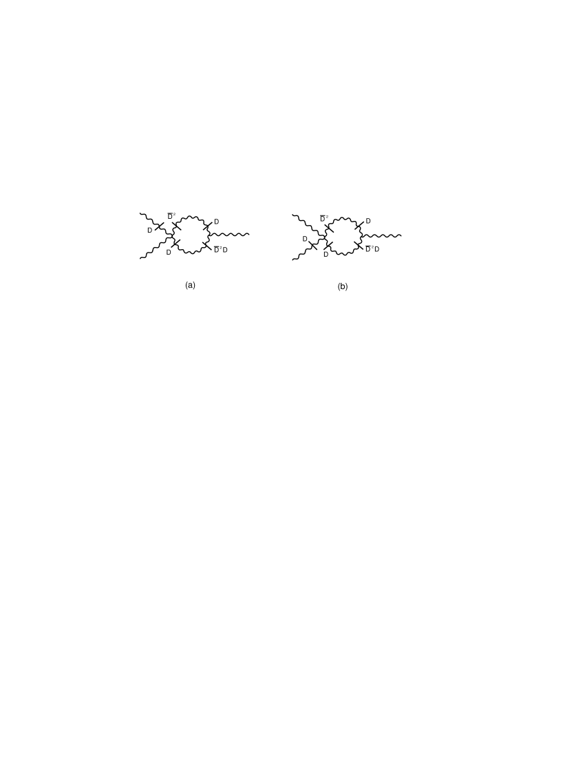
Figure 8: Contributions to $\Gamma^{(1)}_{VVV}$ involving the vertex $\Gamma_{V(DV)(\overline{D}^{2}V)(DV)}^{(0)}$.

In this way we have found that the potentially harmful one-loop diagrams contributing to $\Gamma^{(1)}_{VVV}$ are those depicted in Figs. 5, 6, 7, 8, 9, 10, and 11. To systematize our presentation as well as to facilitate the verification of our calculations, we shall write all the three-point amplitudes $\Gamma_{VVV}^{(1)}$ as follows

$$\Gamma_{VVV}^{(1)}\,=\,\left[\frac{1}{n!}\right]\,\times\,[t]\,\times\,[v]\,\times\,\int\,\left[\frac{d^{4}k}{\left(2\pi\right)^{4}}\,d\theta\right]\,\times\,\left[F_{T}\right]\,\times\,[P]\,\times\,{\mathbb{D}}_{\theta}\,+\,permutations\,.$$ (66)

Here, $1/n!$ comes from the order of the perturbative expansion, $t$ is the topological factor, $v$ is the numerical factor associated with the vertices, $d\theta$ is the fermionic measure, $F_{T}$ is the trigonometric factor provided by the noncommutativity, $P$ is the product of $\theta$-independent factors in the propagators, ${\mathbb{D}}_{\theta}$ is the $\theta$-dependent part of the integrand, and one is to sum over the appropriate permutations of the external momenta.

For the tadpole graph in Fig. 5 one has that $n=t=1$, $v=-g^{3}/36$,

$$F_{T;5}\, = \,\mathcal{V}^{(1)}_{5}\left(k,-k,p_{1},p_{2},p_{3}\right)$$ (67)

$$= \,3\,\cos\left[p_{1}\wedge\left(p_{3}-k\right)+p_{3}\wedge k\right]\sin\left(k\wedge p_{2}\right)$$

$$+ \,3\cos\left[p_{2}\wedge\left(p_{3}-k\right)+p_{3}\wedge k\right]\sin\left(k\wedge p_{1}\right)$$

$$+ \,3\cos\left[p_{2}\wedge\left(p_{1}-k\right)+p_{1}\wedge k\right]\sin\left(k\wedge p_{3}\right)\,,$$

as can be seen from Eq. (38d), $P=-i/k^{2}$, and

$${\mathbb{D}}_{\theta}\, = \,\delta_{12}\,\left[\overline{D}_{1}^{2}D^{\alpha}_{1}D_{2\alpha}\,\left(1-(1-a)\,\frac{1}{k^{2}}\{D_{1}^{2},{\overline{D}}^{2}_{1}\}\right)\delta_{12}\right]V\left(p_{1},\theta_{1}\right)V\left(p_{2},\theta_{1}\right)V\left(p_{3},\theta_{1}\right)$$ (68)

$$= \,\delta_{12}\,\left[\overline{D}_{1}^{2}D^{\alpha}_{1}D_{2\alpha}\,\delta_{12}\right]V\left(p_{1},\theta_{1}\right)V\left(p_{2},\theta_{1}\right)V\left(p_{3},\theta_{1}\right)\,.$$

As in the case of the two-point function the term in the propagator proportional to $(1-a)$ drops out. By putting all these together one ends up with,

$${\Gamma}_{VVV;5}^{\left(1\right)}\left(p_{1},p_{2},p_{3}\right)$$

$$=\,-\frac{ig^{3}}{18}\,\int\frac{d^{4}k}{\left(2\pi\right)^{4}}d^{4}\theta\,\frac{F_{T;5}}{k^{2}}\,V\left(p_{1},\theta\right)V\left(p_{2},\theta\right)V\left(p_{3},\theta\right)\,+\,AP\,,$$ (69)

where $AP$ means that one is to sum over all permutations of the external momenta. By power counting Eq. (IV) is quadratically UV divergent but, on the other hand, Eq. (67) tell us that the planar part vanishes, implying in the absence of UV divergences. Hence, what we have to investigate are the consequences of the UV/IR mechanism fully contained in the nonplanar part. A direct calculation shows that

$${\Gamma}_{VVV;5}^{\left(1\right)}\left(p_{1},p_{2},p_{3}\right)\, = \,-\,\frac{i}{8\pi^{2}}\,\left\{\sin\left(p_{1}\wedge p_{3}\right)\left[\frac{1}{p_{3}\circ p_{3}}-\frac{1}{p_{1}\circ p_{1}}\right]\right.$$ (70)

$$+\sin\left(p_{2}\wedge p_{3}\right)\left[\frac{1}{p_{3}\circ p_{3}}-\frac{1}{p_{2}\circ p_{2}}\right]$$

$$\left.+\sin\left(p_{2}\wedge p_{1}\right)\left[\frac{1}{p_{1}\circ p_{1}}-\frac{1}{p_{2}\circ p_{2}}\right]\right\}\,B\,+\,AP\,.$$

For arriving at Eq. (70) we have used

$$\int\frac{d^{4}k}{\left(2\pi\right)^{4}}\frac{\sin\left(2k\wedge p\right)}{k^{2}}\,=\,0\,,$$ (71a)

$$\int\frac{d^{4}k}{\left(2\pi\right)^{4}}\frac{\cos\left(2k\wedge p\right)}{k^{2}}=\frac{1}{4\pi^{2}p\circ p}\,,$$ (71b)

and

$$B\,\equiv\,g^{3}\int d^{4}\theta\,V\left(p_{1},\theta\right)V\left(p_{2},\theta\right)V\left(p_{3},\theta\right)\,.$$ (72)

It is easy to verify that momentum conservation enforces

$${\Gamma}_{VVV;5}^{\left(1\right)}\left(p_{1},p_{2},p_{3}\right)\,=\,0\,,$$ (73)

implying in the absence of UV/IR infrared divergences as well. One can convince oneself that the trigonometric factor corresponding to the tadpoles involving the vertices $\Gamma_{(\overline{D}^{2}V)(DV)(DV)V}^{(0)}$ and $\Gamma_{(\overline{D}DV)({\overline{D}}V)(DV)V}^{(0)}$ (see Fig. 2) are proportional to $\sin(p_{1}\wedge p_{2})$ and, therefore, the would be linear UV/IR infrared divergence is softened and becomes harmless.

The diagrams in Fig. 6 have in common the four-point vertex $\Gamma_{(\overline{D}^{2}DV)(DV)VV}^{(0)}$. We focus first on diagram (a). We have that $n=2$, $t=4$, $v=-ig^{3}/12$, and

$$P\,=\,\frac{(-i)^{2}}{k^{2}\,(k-p_{3})^{2}}\,.$$ (74)

For the trigonometric factors an straightforward calculation yields

$$F_{T;6{\rm a}}\,=\,-2\,\cos(p_{1}\wedge p_{2})\,F_{T}^{odd}\,+\,2\,\sin(p_{1}\wedge p_{2})\,F_{T;6{\rm a}}^{even}\,,$$ (75)

where

$$F_{T}^{odd}\,=\,-\,\frac{1}{4}\,\left[\sin\left(2k\wedge p_{1}\right)\,+\,\sin\left(2k\wedge p_{2}\right)\,+\,\sin\left(2k\wedge p_{3}\right)\right]\,,$$ (76a)

$$F_{T;6{\rm a}}^{even}\,=\,-\,\frac{1}{4}\,\left[\cos\left(2k\wedge p_{1}\right)\,-\,\cos\left(2k\wedge p_{2}\right)\right]\,.$$ (76b)

As for the $\theta$ dependent factors, we obtain,

$${\mathbb{D}}_{\theta;6{\rm a}}\, = \,-\,2\,\left[(k-p_{3})^{2}\,V(p_{3},\theta_{2})\,+\,({\not\!k}-{\not\!p_{3}})_{\alpha{\dot{\alpha}}}\,\left({\overline{D}}^{{\dot{\alpha}}}D^{\alpha}V(p_{3},\theta_{2}\right)\,+\,\cdots\right]\,$$ (77)

$$\times \,\delta_{12}\,V(p_{1},\theta_{1})\,V(p_{2},\theta_{1})\,,$$

where we omitted all terms leading to contributions which are at the most logarithmically divergent. Observe that the term proportional to $(1-a)$ in the $V$-propagator does not contribute again.

Power counting says that the diagram (a) is UV quadratically divergent although, as before, the corresponding trigonometric factor does not contain a planar part. The amplitude is, then, UV finite and we concentrate on studying the outcomes of the UV/IR mechanism. After expanding Eq. (74) around $p_{3}=0$, the expression for the amplitude associated with the graph (a) can be cast

$$\Gamma_{VVV;6{\rm a}}^{(1)}\, = \,\frac{ig^{3}}{6}\,\int\frac{d^{4}k}{\left(2\pi\right)^{4}}\,d\theta\,F_{T;6{\rm a}}\,\left[\frac{1}{(k^{2})^{2}}\,+\,2\,p^{\mu}_{3}\,\frac{k_{\mu}}{(k^{2})^{3}}\,+\,\cdots\right]$$

$$\times \,\left[(k-p_{3})^{2}\,V(p_{3},\theta)\,+\,({\not\!k}-{\not\!p_{3}})_{\alpha{\dot{\alpha}}}\,\left({\overline{D}}^{{\dot{\alpha}}}D^{\alpha}V(p_{3},\theta)\right)\,+\,\cdots\right]$$

$$\times \,V(p_{1},\theta)\,V(p_{2},\theta)\,+\,CP\,,$$ (78)

where $CP$ means sum over cyclic permutations of the external momenta. By collecting terms of equal power in $k$, we write

$$\Gamma_{VVV;6{\rm a}}^{(1)}\,\equiv\,\gamma_{6{\rm a}}^{[2]}\,+\,\gamma_{6{\rm a}}^{[1]}\,+\,LDT\,,$$ (79)

where

$$\gamma_{6{\rm a}}^{[2]}\,=\,\left(\frac{ig^{3}}{6}\right)\,2\,\sin(p_{1}\wedge p_{2})\,\int\frac{d^{4}k}{\left(2\pi\right)^{4}}\,d\theta\,F_{T;6{\rm a}}^{even}\frac{1}{k^{2}}\,V(p_{1},\theta)V(p_{2},\theta)V(p_{3},\theta)\,+\,CP\,,$$ (80)

$$\gamma_{6{\rm a}}^{[1]}\, = \,-\,\left(\frac{ig^{3}}{6}\right)\,2\,\cos(p_{1}\wedge p_{2})\,\int\frac{d^{4}k}{\left(2\pi\right)^{4}}\,d\theta\,F_{T}^{odd}\frac{1}{\left(k^{2}\right)^{2}}$$

$$\times \,{\not\!k}_{\alpha{\dot{\alpha}}}\left({\overline{D}}^{{\dot{\alpha}}}D^{\alpha}V(p_{3},\theta)\right)\,V(p_{1},\theta)V(p_{2},\theta)\,+\,CP\,,$$ (81)

and the superscript makes reference to the power of $k$.

A word of caution is here in order. Two terms of the form

$$p_{3}^{\mu}\,\cos(p_{1}\wedge p_{2})\,\int\,\frac{d^{4}k}{\left(2\pi\right)^{4}}\,F_{T}^{odd}\frac{k_{\mu}}{\left(k^{2}\right)^{2}}\,B\,,$$ (82)

occur in the right hand side of Eq. (IV). Expressions of this type arise as a result of expanding the factor $P$ (see Eq. (66)) around zero external momenta. In the present case they cancel out between themselves, giving no contribution to linear UV/IR infrared divergences. However, we would like to remark that individually they also vanish, since after performing the sum over the permutations of the external momenta one finds

$$\left(p_{1}\,+\,p_{2}\,+\,p_{3}\right)^{\mu}\,\cos(p_{1}\wedge p_{2})\,\int\,\frac{d^{4}k}{\left(2\pi\right)^{4}}\,F_{T}^{odd}\frac{k_{\mu}}{\left(k^{2}\right)^{2}}\,B\,,$$ (83)

which is set to zero by momentum conservation.

By carrying out the momentum integrals in Eqs. (80) and (IV) and after $D$-algebra rearrangements, one obtains, respectively,

$$\gamma_{6{\rm a}}^{[2]}\,=\,-\,\left(\frac{i}{12}\right)\,\sin(p_{1}\wedge p_{2})\,\frac{1}{4\pi^{2}}\left(\frac{1}{p_{1}\circ p_{1}}\,-\,\frac{1}{p_{2}\circ p_{2}}\right)\,B\,+\,CP$$ (84)

and

$$\gamma_{6{\rm a}}^{[1]}\,=\,4\,\left(\frac{i}{6}\right)\,\cos(p_{1}\wedge p_{2})\,I^{\mu}(p_{1},p_{2},p_{3})\,N_{\mu}(p_{1},p_{2},p_{3})\,.$$ (85)

Here,

$$N_{\mu}(p_{1},p_{2},p_{3})\,\equiv g^{3}\,\left(\sigma_{\mu}\right)_{\alpha{\dot{\alpha}}}\int d\theta\left(D^{\alpha}V(p_{1},\theta)\,{\overline{D}}^{{\dot{\alpha}}}V(p_{3},\theta)\,V(p_{2},\theta)\,+\,AP\right)\,,$$ (86)

while $I^{\mu}$ was already defined in Eq. (61).

After recalling momentum conservation one concludes that

$$\gamma_{6{\rm a}}^{[2]}\,=\,0\,.$$ (87)

Thus we are left with a harmful linear UV/IR infrared divergence in $\Gamma_{VVV;6{\rm a}}^{(1)}$ given at Eq. (85).

The diagrams (b), (c), and (d) in Fig. 6 have in common that the terms proportional to $(1-a)$ drop out, as in the case of diagram (a). Since $F_{T;6{\rm b}}\,=\,-\,F_{T;6{\rm a}}$, graph (b) also has no planar part. As for graphs (c) and (d) they have a logarithmically divergent planar part which demands UV renormalization. For all of them, the nonplanar contribution $\gamma^{[2]}$ is absent. We found that

$$\sum_{j=6{\rm b}}^{6{\rm d}}\,\gamma_{j}^{[1]}\,=\,3\,\left(\frac{i}{6}\right)\,\cos(p_{1}\wedge p_{2})\,I^{\mu}(p_{1},p_{2},p_{3})\,N_{\mu}(p_{1},p_{2},p_{3})\,.$$ (88)

On the other hand, the graphs (e), (f) and (g) turn out to be proportional to $(1-a)$. While (e) has no planar part, (f) and (g) exhibit a logarithmic UV divergence. Again, $\gamma^{[2]}=0$. We end up with

$$\sum_{j=6{\rm e}}^{6{\rm g}}\,\gamma_{j}^{[1]}\,=\,(1-a)\,\left(\frac{ig^{3}}{6}\right)\,\cos(p_{1}\wedge p_{2})\,I^{\mu}(p_{1},p_{2},p_{3})\,N_{\mu}(p_{1},p_{2},p_{3})\,.$$ (89)

Therefore,

$$\sum_{j=6{\rm a}}^{6{\rm g}}\Gamma^{(1)}_{VVV;j}\,=\,(8-a)\,\left(\frac{i}{6}\right)\,\cos(p_{1}\wedge p_{2})\,I^{\mu}(p_{1},p_{2},p_{3})\,N_{\mu}(p_{1},p_{2},p_{3})\,+\,LDT\,,$$ (90)

where the linear UV/IR infrared divergence, arising from the diagrams in Fig. 6, is explicitly given.

We move next into computing the diagrams in Fig. 7. Unlike those in Fig. 6 they involve the four-point vertex $\Gamma_{V(DV)(\overline{D}V)({\overline{D}}DV)}^{(0)}$ (see Eq. (33b)). An analysis quite similar to that already presented enables one to conclude that the planar part has, at the most, a logarithmic UV divergence. A linear UV/IR infrared divergence is present in each graph but, nevertheless, cancels. That is

$$\sum_{j=7{\rm a}}^{7{\rm p}}\,\Gamma^{(1)}_{VVV;j}\,=\,LDT\,.$$ (91)

The diagrams in Fig. 8 involve the last four point vertex $\Gamma_{V(DV)({\overline{D}}^{2}V)(DV)}^{(0)}$ quoted in Eq. (33c). In the planar sector the situation is as in the case of the diagrams in Fig. 7, only logarithmic UV divergences show up. In the nonplanar sector the linear UV/IR infrared divergences do not cancel and the final form for the corresponding amplitude is

$$\sum_{j=8{\rm a}}^{8{\rm b}}\Gamma^{(1)}_{VVV;j}\,=\,-\,6\,a\,\left(\frac{i}{6}\right)\,\cos(p_{1}\wedge p_{2})\,I^{\mu}(p_{1},p_{2},p_{3})\,N_{\mu}(p_{1},p_{2},p_{3})\,+\,LDT\,.$$ (92)

We turn next into evaluating the graphs in Fig. 9. All of them have in common, up to an overall sign, the trigonometric factor

$$F_{T;9}\,=\,\cos(p_{1}\wedge p_{2})\,F_{T}^{odd}\,+\,\sin(p_{1}\wedge p_{2})\,F_{T;9}^{even}\,,$$ (93)

where $F_{T}^{odd}$ was defined in Eq. (76a) and

$$F_{T;9}^{even}\,=\,-\,\frac{1}{4}\,\left[1\,-\,\cos(2k\wedge p_{1})\,+\,\cos(2k\wedge p_{2})\,-\,\cos(2k\wedge p_{3})\right]\,.$$ (94)

Hence, the planar part does not vanish. From the $D$-algebra follows that quadratic UV divergences only arise in graphs (a) to (d) and are taken care by dimensional regularization. For all graphs in Fig. 9, linear UV divergences are killed by symmetric integration, while the logarithmic ones are absorbed through renormalization.

In principle there is nothing that could prevent the appearance of quadratic UV/IR infrared divergences, from graphs (a) to (d), in view of $F_{T;9}^{even}\,\neq\,0$. Nevertheless, the presence of $\sin(p_{1}\wedge p_{2})$ in Eq. (93) lowers the degree of this divergence at least to linear. The softening mechanism, mentioned at the beginning of this section, is again at work. For each graph, one can verify that the UV/IR linear infrared divergences arising through this mechanism are of the form

$$\sin(p_{1}\wedge p_{2})\left(\frac{1}{p_{1}\circ p_{1}}\,-\,\frac{1}{p_{2}\circ p_{2}}\,+\,\frac{1}{p_{3}\circ p_{3}}\right)\,,$$ (95)

and therefore cancel after symmetrizing in the external momenta.

On the other hand, for all the graphs, there are linear infrared divergences which are the UV/IR counterparts of the would be linear UV divergences. These divergences cancel when summing up over all graphs in Fig. 9.

For the ghost graphs (a) and (b) in Fig. 10 the trigonometric factors are found to read

$$F_{T;10{\rm a}}\,=\,F_{T;10{\rm b}}\,=\,-2\,\cos(p_{1}\wedge p_{2})\,F_{T}^{odd}\,+\,2\,\sin(p_{1}\wedge p_{2})\,F_{T;6{\rm a}}^{even}\,=\,F_{T;6{\rm a}}\,,$$ (96)

whereas for the others diagrams in Fig. 10 one has

$$F_{T;10^{\prime}}\,=\,-\,\cos(p_{1}\wedge p_{2})\,F_{T}^{odd}\,-\,\sin(p_{1}\wedge p_{2})\,F_{T;9}^{even}\,=\,-\,F_{T;9}\,.$$ (97)

The $D$-algebra signalizes again the presence of quadratic, linear and logarithmic UV divergences in graphs (c) to (f) in Fig. 10, since their trigonometric factor possesses a nonvanishing planar part. As it already happens in connection with the graphs in Fig. 9, the linear UV/IR infrared divergences arising from the softening mechanism vanish for each graph. The remaining linear divergences do not cancel and we obtain

$$\sum_{j=10{\rm a}}^{10{\rm f}}\Gamma^{(1)}_{VVV;j}\,=\,-\,4\,\left(\frac{i}{6}\right)\,\cos(p_{1}\wedge p_{2})\,I^{\mu}(p_{1},p_{2},p_{3})\,N_{\mu}(p_{1},p_{2},p_{3})\,+\,LDT\,.$$ (98)

To summarize, in NCSQED₄ and for ${\cal N}=1$, the one-loop corrections to the three-point gauge superfield function are afflicted by linear UV/IR infrared singularities. By collecting the calculations presented in this section, Eqs. (73), (90), (91), (92), and (98), we conclude that the amplitude can be cast in the following form

$$\Gamma^{(1)}_{VVV}=\,(4\,-\,7a)\,\left(\frac{i}{6}\right)\,\cos(p_{1}\wedge p_{2})\,I^{\mu}(p_{1},p_{2},p_{3})\,N_{\mu}(p_{1},p_{2},p_{3})\,+\,LDT\,.$$ (99)

As can be seen, for the gauge $a=4/7$ the three-point $V$ function is free of linear UV/IR infrared divergences. To phrase it differently, these divergences are localized in the gauge sector and are a gauge artifact.

This result is not altered by the addition of one chiral matter superfield (see Fig. 11). In fact, the contribution of the tadpole graph (a) is proportional to that of the $V$-tadpole in Eq. (73). Furthermore, the amplitudes corresponding to the graphs (b) and (c) are proportional, respectively, to those of the graphs (a) and (c) of Fig. 10. The linear UV/IR infrared divergences resulting from the quadratic UV divergences, via the softening mechanism, cancel out for each graph. As for the remaining linear UV/IR infrared divergences, in diagrams (b) and (c), the numerical coefficients are such as to secure their cancellation. The generalization of these results to ${\cal N}=4$ is straightforward.

V Conclusions

This work was dedicated to establish the consistency of NCSQED₄ within the covariant superfield formalism. As a first step, we generalized the analysis of the two-point gauge field function presented in bichl by extending their results to an arbitrary covariant gauge and for any matter content.

Our main contribution consists of a detailed study of the divergence structure of the one-loop three-point function of the gauge superfield. The superfield formulation in an arbitrary covariant gauge, represents a significative improvement with respect to the component field calculation presented in Mat ; RR1 for the same problem. At the very least, here supersymmetry is kept operational at all stages of the calculation. Unlike in the component formulation, we have found a nonvanishing result for the linear UV/IR infrared divergences which are, nevertheless, a gauge artifact. The situation resembles that encountered in QED₄ where the infrared divergences disappear from the full two-point fermion Green function in a particular covariant gauge (Yennie’s gauge Yennie ).

The present work also plays a relevant role within the background field formalism. Indeed, the computation of higher loop corrections to the results encountered in Za1 ; Zanon will necessarily demand the insertion of the three-point $V$-function calculated in the superfield covariant formalism (see Fig. 4). Our conclusion that the linear UV/IR infrared singularities are placed in the gauge sector implies that higher order loop corrections to the background field strength function will not be afflicted by harmful UV/IR infrared singularities.

Acknowledgements. This work was partially supported by Fundação de Amparo à Pesquisa do Estado de São Paulo (FAPESP) and Conselho Nacional de Desenvolvimento Científico e Tecnológico (CNPq). H. O. G. and V. O. R. also acknowledge support from PRONEX under contract CNPq 66.2002/1998-99. A. Yu. Petrov has been supported by FAPESP, project No. 00/12671-7.

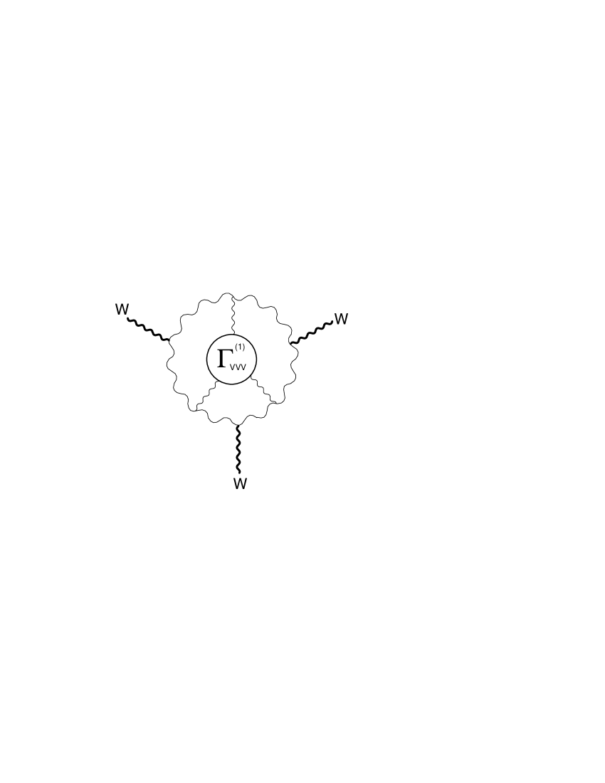
Figure 4: An example of higher order correction to the three-point $W$ function including the one-loop three-point $V$ function.

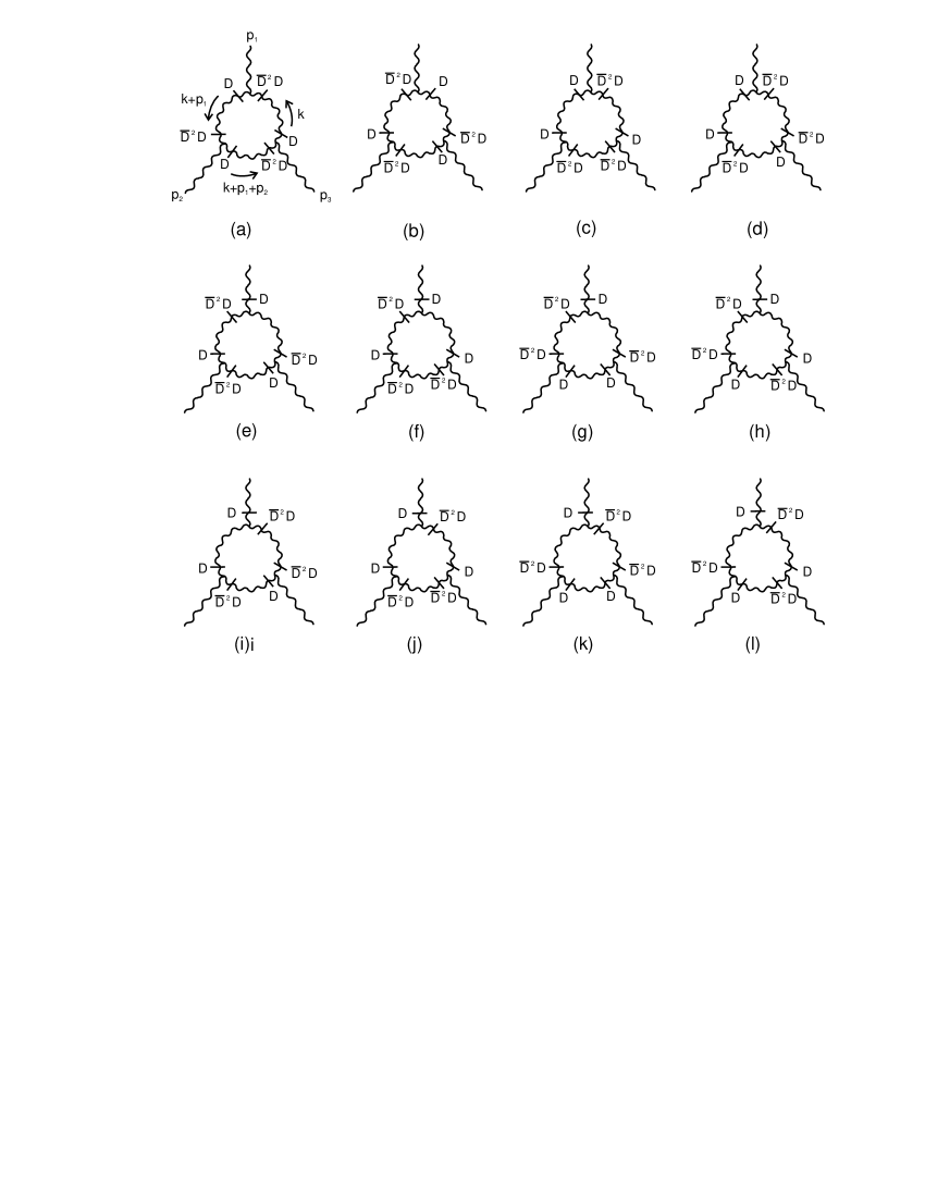
Figure 9: Contributions to $\Gamma^{(1)}_{VVV}$ involving the trilinear vertex only.

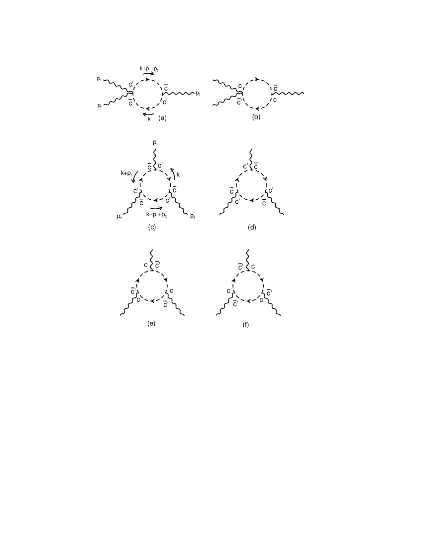
Figure 10: Ghost contributions to $\Gamma^{(1)}_{VVV}$.

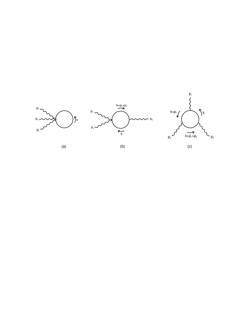
Figure 11: Matter contributions to $\Gamma^{(1)}_{VVV}$.

References

- (1) N. Seiberg, E. Witten, JHEP 09, 032 (1999).
- (2) M. Douglas, N. A. Nekrasov, Rev. Mod. Phys. 73, 977 (2002).
- (3) R. Szabo, Phys. Rept. 378, 207 (2003).
- (4) M. Gomes in Proceedings of the XI Jorge André Swieca Summer School, Particles and Fields, G. A. Alves, O. J. P. Éboli and V. O. Rivelles eds, World Scientific Pub. Co, 2002; H. O. Girotti, “Noncommutative Quantum Field Theories”, hep-th/0301237.
- (5) S. Minwalla, M. van Raamsdonk, N. Seiberg, JHEP 02, 020 (2000).
- (6) A. Matusis, L. Susskind, N. Toumbas, JHEP 12, 002 (2000).
- (7) F. Ruiz Ruiz, Phys. Lett. B502, 274 (2001).
- (8) To avoid confusion with the standard infrared divergences, those originating through the UV/IR mechanism will be referred to as UV/IR infrared divergences.
- (9) H. O. Girotti, M. Gomes, V. O. Rivelles, A. J. da Silva, Nucl. Phys. B587, 299 (2000).
- (10) I. L. Buchbinder, M. Gomes, A. Yu. Petrov, V. O. Rivelles, Phys. Lett. B517, 191 (2001).
- (11) H. O. Girotti, M. Gomes, A. Yu. Petrov, V. O. Rivelles, A. J. da Silva. Phys. Lett. B521, 119 (2001).
- (12) H. O. Girotti, M. Gomes, A. Yu. Petrov, V. O. Rivelles, A. J. da Silva, Phys. Rev. D 67 125003 (2003).
- (13) M. Hayakawa. Phys. Lett. B478, 394 (2000); “Perturbative analysis of infrared and ultraviolet aspects of noncommutative QED on ”, hep-th/9912167.
- (14) M. M. Sheikh-Jabbari, JHEP 08, 045 (2000).
- (15) L. Bonora, M. Salizzoni. Phys. Lett. B504, 80 (2001); L. Bonora, M. Schnabl, M. M. Sheikh-Jabbari, A. Tomasiello, Nucl. Phys. B589, 461 (2000).
- (16) S. Ferrara, M. A. Lledo, JHEP 05, 008 (2000).
- (17) Z. Guralnik, S. Y. Pi, R. Jackiw, A. P. Polychronacos, Phys. Lett. B517, 450 (2001).
- (18) A. Armoni. Nucl. Phys. B593, 229 (2001); A. Armoni, E. Lopez. Nucl. Phys. B632, 240 (2002).
- (19) L. Jiang, E. Nicholson, Phys. Rev. D 65, 105020 (2002); E. Nicholson, Phys. Rev. D 66, 105018 (2002).
- (20) A. A. Bichl, M. Ertl, A. Gerhold, J. M. Grimstrup, H. Grosse, L. Popp, V. Putz, M. Schweda, R. Wulkenhaar, “Non-commutative U(1) Super-Yang-Mills Theory: Perturbative Self-Energy Corrections”, hep-th/0203141.
- (21) D. Zanon, Phys. Lett. B502, 265 (2001).
- (22) D. Zanon, Phys. Lett. B504, 101 (2001); M. Pernici, A. Santambrogio, D. Zanon, Phys. Lett. B504, 131 (2001); A. Santambrogio, D. Zanon, JHEP 01, 024 (2001).
- (23) S. J. Gates, M. T. Grisaru, M. Rocek, W. Siegel, Superspace or One Thousand and One Lessons in Supersymmetry (Benjamin/Cummings, 1983).
- (24) In this paper, we shall follow the conventions in Ref. SGRS .
- (25) I. L. Buchbinder and S. M. Kuzenko, Ideas and Methods of Supersymmetry and Supergravity, IOP, Bristol and Philadelphia, 1998.
- (26) See, for instance Refs. Nekr ; Szabo ; Girotti11 .
- (27) D. R. Yennie, S. C. Frautschi, and H. Suura, Ann. Phys. 13, 379 (1961).