hep-th/0309135

UT-03-28

Boundary States for Supertubes in
Flat Spacetime and Gödel Universe
Hiromitsu Takayanagi

Department of Physics, Faculty of Science, University of Tokyo
Hongo 7-3-1, Bunkyo-ku, Tokyo, 113-0033, Japan

We construct boundary states for supertubes in the flat spacetime. The T-dual objects of supertubes are moving spiral D1-branes (D-helices). Since we can obtain these D-helices from the usual D1-branes via null deformation, we can construct the boundary states for these moving D-helices in the covariant formalism. Using these boundary states, we calculate the vacuum amplitude between two supertubes in the closed string channel and read the open string spectrum via the open closed duality. We find there are critical values of the energy for on-shell open strings on the supertubes due to the non-trivial stringy correction. We also consider supertubes in the type IIA Gödel universe in order to use them as probes of closed timelike curves. This universe is the T-dual of the maximally supersymmetric type IIB PP-wave background. Since the null deformations of D-branes are also allowed in this PP-wave, we can construct the boundary states for supertubes in the type IIA Gödel universe in the same way. We obtain the open string spectrum on the supertube from the vacuum amplitude between supertubes. As a consequence, we find that the tachyonic instability of open strings on the supertube, which is the signal of closed time like curves, disappears due to the stringy correction.

1 Introduction

In the resent development of the string theory, D-branes played an important role. Especially, since D-branes are non-perturbative solitons, we have revealed many non-perturbative aspects in the string theory by studying the dynamics of D-branes.

Now although D-branes have tension, it is known that in a type IIA string theory, tubular D2-branes in the flat spacetime can be stable by adding proper electric and magnetic gauge flux on them. These D2-D0-F1 bound states are called ‘supertubes’ [1]. Supertubes also preserve 8 supercharges in spite of its curved configuration. An important feature of supertubes is that we can interpret a supertube as a ‘blown up’ object of D0-branes (see [2] for the matrix description of D-particles). Therefore it is interesting to study the blow up process from D0-branes to supertubes. In this paper we would like to study this process in the string theory. Since the background RR-flux is not needed in contrast with the Myers’ effect [3], a dielectric effect of D-branes in the presence of the background RR-flux, there is a possibility to treat this process in the NSR superstring formulation and indeed it is possible as we will see.

Taking the T-duality in the direction in which the supertube is extended, we can obtain a moving spiral D1-brane (D-helix) from the supertube as is claimed in [4]. The main idea used in this paper is that we can get this moving D-helix from a static D1-brane via ‘null deformation’ [5, 6, 7, 8] (see also [9] for more generalized cases), the deformation only in the $x^{+}$ direction. Therefore the blow up process corresponds to the null deformation in the T-dual picture.

In this paper we would like to follow this null deformation in the string theory using the boundary state formalism. In the boundary state formalism, D-branes are treated as the initial (final) states of closed strings and these states are called boundary states. We will use this formalism because the situation becomes simpler. While the time evolution of open strings on supertubes is non-trivial because of boundary interactions, closed strings propagate trivially once they are emitted at the boundary. Due to this advantage, we can treat the null deformation of boundary states in the covariant formalism [5, 10]. We express the null deformation (the blow up in the T-dual picture) as deformation operators (Wilson loop) on the boundary and as a consequence, we can obtain boundary states for supertubes. We would like to stress that we can treat these boundary states exactly without light cone gauge fixing, i.e., without breaking the conformal invariance of the string world sheet. In the string theory, we highly depend on the conformal invariance of the world sheet to calculate string scattering amplitudes. Therefore we need to treat strings covariantly for further analyses.

D-branes are also useful for studying stringy effects on geometries because we can use them as probes [11]. Since supertubes have tubular form, we can analyze stringy effects near a certain curve using supertubes as probes. Especially they are useful in studying closed timelike curves (CTCs) in Gödel universe [12]. The main motivation of studying Gödel universe is to find out fates of backgrounds with CTCs and it is interesting to study this problem in the string theory [13, 14, 15, 16, 17, 18, 19, 20, 21, 22, 23, 24]. In this sense, the supersymmetric type IIA Gödel universe [15] will be a good example. This is because we can obtain the universe via T-duality from the (compactified) maximally supersymmetric type IIB pp-wave [25] as is claimed in [15]. Since we can construct an exactly solvable string theory on the maximally supersymmetric type IIB pp-wave background [26], we can also treat the type IIA Gödel universe in the string theory [16]. This background also has 20 supersymmetries and we can expect a high stability against quantum corrections.

In this paper we would also like to consider supertubes in the supersymmetric type IIA Gödel universe. We put a supertube whose worldvolume is along a CTC in order to use it as a probe [18, 19, 22, 23]. As before its T-dual is a moving D-helix, a null deformed D1-brane, in the the maximally supersymmetric type IIB PP-wave background. As claimed in [27], the null deformations of D-branes are also allowed in this PP-wave. We will find that we can construct the boundary states for D-helices in this background in the same way as in the flat spacetime. We will compute the vacuum amplitude between supertubes and obtain the open string spectra on them from which we can read the stringy correction to closed timelike curves.

This paper is organized as follows. In section 2 we construct the boundary states for the supertubes in the flat background and consider the open string spectra on them. We also construct the boundary states for deformed supertubes [28, 29, 30] (see also [31, 32, 33] for the supersymmetric D2-anti D2 brane system which we can obtain by deforming a supertube). In section 3 we consider supertubes in type IIA Gödel universe. We construct boundary states for them in a similar manner and obtain open string spectra on them. In section 4 we give a brief summary of our results and draw conclusions.

2 Boundary State for Supertube in Flat Spacetime

In this section we will denote the world volume directions of the supertube as $(t,\phi,\tilde{y})$. The supertube has the gauge flux $F_{t\tilde{y}}=-1$ and $F_{\phi\tilde{y}}=\mbox{constant}$. Though one might think the electric field is at the critical value, it is not the case because of the non zero magnetic flux. To see the further property of supertubes, let us compactify the $\tilde{y}$ direction with the radius $\tilde{R}$. When a supertube consists of $N$ D2-branes, $k$ D0-branes and $q$ F-strings, which we will call the $(N,k)$ supertube, magnetic flux and the radius of the supertube denoted by $\rho$ are quantized as follows

$$F_{\phi\tilde{y}}=\frac{\alpha^{\prime}}{\tilde{R}}\frac{k}{N},\quad\rho^{2}=g_{s}\frac{|qk|\alpha^{\prime\frac{3}{2}}}{N^{2}\tilde{R}},$$ (2.1)

where $g_{s}$ is the coupling constant for closed strings. The important feature is that the tension of this supertube equals the sum of the tension of $|q|$ F-strings and $|k|$ D0-branes. Therefore we can interpret supertube as the ‘blown up’ D0-branes.

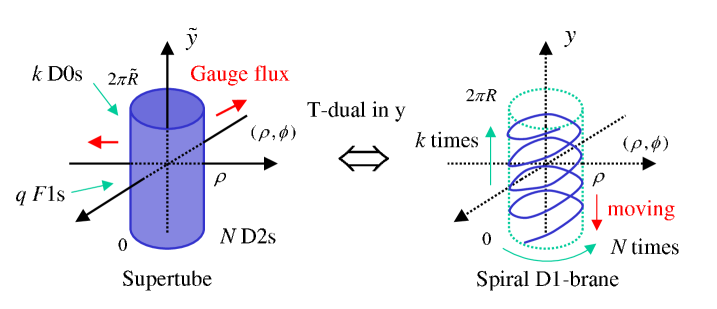
Figure 1: Supertube and Spiral D1-brane

Taking a T-duality in the $\tilde{y}$ direction, we can treat the supertube more easily. As claimed in [4], a T-dualized object of the supertube is a moving ‘D-helix’, a spiral D1-brane, wound $k$ times in the $y$ direction and $N$ times in the $\phi$ direction (see fig.1). We can check this fact by treating D-branes as boundary conditions of open strings. Although we will consider them in a bosonic string theory for simplicity, we can easily extend obtained results to super string cases as is discussed later. Remembering that the (mixed) Neumann boundary condition is given by

$$G_{\mu\nu}\partial_{N}X^{\nu}+(B_{\mu\nu}+F_{\mu\nu})\partial_{D}X^{\nu}=0,$$ (2.2)

we can write down the boundary conditions for the supertube as follows

$$\begin{split}\mu=t:&\quad-\partial_{N}t-\partial_{D}\tilde{y}=0,\\ \mu=\phi:&\quad+\rho^{2}\partial_{N}\phi+b\partial_{D}\tilde{y}=0,\\ \mu=\tilde{y}:&\quad\partial_{N}\tilde{y}+\partial_{D}t-b\partial_{D}\phi=0,\\ \mu=\rho:&\ \quad\partial_{D}\rho=0,\end{split}$$ (2.3)

where we defined $F_{\phi\tilde{y}}=b$. Taking the T-duality in $\tilde{y}$ direction and defining light cone directions as $x^{+}=t+y$, $x^{-}=\frac{1}{2}(t-y)$, these change to

$$\partial_{N}x^{+}=0,\quad\partial_{N}x^{-}-\frac{\rho^{2}}{b}\partial_{N}\phi=0,\quad\partial_{D}(\phi-\frac{1}{b}x^{+})=0,\quad\partial_{D}\rho=0,\quad b=R\frac{k}{N},$$ (2.4)

where $R=\alpha^{\prime}/\tilde{R}$ is the radius of the y direction. Eq.(2.4) is just the conditions for the moving D-helix in fig.1.

Now eq.(2.4) tells us that we can obtain this moving D-helix from usual D1-branes extended in the $y$ direction via ‘null deformation’ [5, 6, 7, 8, 9], i.e., a deformation only in the $x^{+}$ direction. Noticing this fact we would like to treat D-branes in the boundary state formalism and construct the boundary states for supertubes via the null deformation [5, 10] in the next section. First let us treat the case of $k=1$ for simplicity because the number of segments of D1-brane is one .

2.1 Boundary State for $k=1$ Supertube and Vacuum Amplitude

As we have reviewed in the previous section, a supertube is described as a moving spiral D1-brane (D-helix) in the T-dualized background. Here we would like to construct the boundary state for this D-helix and calculate the vacuum amplitude.

Using the formalism in [34], we can get the boundary state for the D-helix wound $(N,1)$ times in the $(\phi,y)$ directions (denoted as $|N,1\rangle$) by multiplying one static D1-brane $|D1\rangle$ by the proper Wilson loop-like operator. That is

$$|N,1\rangle=e^{-\frac{i}{2\pi\alpha^{\prime}}\int_{0}^{2\pi}d\sigma V_{N,1}}|D1\rangle,\quad V_{N,1}=\rho\cos(\frac{NX^{+}}{R})\partial_{\tau}X^{1}+\rho\sin(\frac{NX^{+}}{R})\partial_{\tau}X^{2},$$ (2.7)

where we used the relation $b=\frac{Rk}{N}$. Notice that this boundary state preserves the boundary conformal invariance including renormalization because the deformation is null [5] (see also [35] for the proof for supertubes in the context of the boundary conformal field theory). We can also rewrite it using oscillators as follows

$$|N,1\rangle=\prod_{m=1}^{\infty}\exp\Big{[}-\frac{m}{\alpha^{\prime}}V^{i}_{m}V^{i}_{-m}-i\sqrt{\frac{2}{\alpha^{\prime}}}(V^{i}_{m}\alpha^{i}_{-m}+V^{i}_{-m}\tilde{\alpha}^{i}_{-m})\Big{]}|D1\rangle,$$ (2.8)

where we defined

$$V^{1}_{m}(X^{+})\equiv\frac{1}{2\pi}\int_{0}^{2\pi}d\sigma\rho\cos(\frac{X^{+}}{b})e^{im\sigma},\quad V^{2}_{m}(X^{+})\equiv\frac{1}{2\pi}\int_{0}^{2\pi}d\sigma\rho\sin(\frac{X^{+}}{b})e^{im\sigma}.$$ (2.9)

Notice that $\alpha^{+}_{m}$’s commute each other. Then $V^{i}_{m}$ is well defined.

Now let us compute the following vacuum amplitude between the same $(N,1)$ D-helix

$$Z=\langle N,1|\Delta|N,1\rangle=\frac{\alpha^{\prime}}{2}\int_{0}^{\infty}ds\langle N,1|e^{-sH}|N,1\rangle\equiv\int_{0}^{\infty}ds{\cal A}(s),$$ (2.10)

where $\Delta$ is a closed string propagator and the function ${\cal A}(s)$ is given by

$${\cal A}(s)=\frac{\alpha^{\prime}}{2}\langle N,1|e^{-sH}|N,1\rangle=\frac{\alpha^{\prime}}{2}\langle D1|e^{\frac{i}{2\pi\alpha^{\prime}}\int_{0}^{2\pi}d\sigma V_{N,1}}e^{-sH}e^{-\frac{i}{2\pi\alpha^{\prime}}\int_{0}^{2\pi}d\sigma V_{N,1}}|D1\rangle.$$ (2.11)

As is shown in [10], we can neglect massive modes in the $x^{+}$ direction, i.e., $\alpha^{+}_{m}$ for $m\neq 0$, in evaluating this amplitude. Considering only zero modes, $V^{i}_{m}$ has the following simple form

$$V^{1}_{\pm Nw}=\frac{\rho}{2}e^{\mp i\frac{Nx^{+}}{R}},\quad V^{2}_{\pm Nw}=\pm i\frac{\rho}{2}e^{\mp i\frac{Nx^{+}}{R}},\quad\mbox{otherwise zero},$$ (2.12)

where $w$ denotes the winding number in the $y$ direction, i.e., $X^{+}=x^{+}+Rw\sigma+\cdots$. Notice that this simpleness is due to the periodicity of the function $V^{i}_{N,1}$ under the shift $X^{+}\rightarrow X^{+}+2\pi R$. Then we can use the following effective boundary state in calculating the vacuum amplitude

$$|N,1\rangle\sim\exp\Big{[}-\frac{|Nw|}{\alpha^{\prime}}V^{i}_{|Nw|}V^{i}_{-|Nw|}-i\sqrt{\frac{2}{\alpha^{\prime}}}(V^{i}_{|Nw|}\alpha^{i}_{-|Nw|}+V^{i}_{-|Nw|}\tilde{\alpha}^{i}_{-|Nw|})\Big{]}|D1\rangle.$$ (2.13)

Employing the formula

$$\begin{split}&\langle 0|e^{-\frac{1}{m}\alpha_{m}\tilde{\alpha}_{m}}e^{(f^{(2)}_{-m}\alpha_{m}+f^{(2)}_{m}\tilde{\alpha}_{m})}e^{-s(\alpha_{-m}\alpha_{m}+\tilde{\alpha}_{-m}\tilde{\alpha}_{m})}e^{(f^{(1)}_{m}\alpha_{-m}+f^{(1)}_{-m}\tilde{\alpha}_{-m})}e^{-\frac{1}{m}\alpha_{-m}\tilde{\alpha}_{-m}}|0\rangle\\ &\ \ =\frac{1}{1-e^{-2ms}}\exp\Bigl{(}-\frac{m}{e^{2ms}-1}\bigl{[}|f^{(1)}_{m}|^{2}+|f^{(2)}_{m}|^{2}-e^{ms}(f^{(1)}_{m}f^{(2)}_{-m}+f^{(1)}_{-m}f^{(2)}_{m})\bigr{]}\Bigr{)},\end{split}$$ (2.14)

which can be shown by repeatedly applying the Baker-Campbell-Hausdorff’s formula ($f^{(1,2)}_{m}(=f^{(1,2)*}_{-m})$ are any constants), we obtain the following vacuum amplitude

$${\cal A}(s)=\frac{{\cal N}}{(2\pi\alpha^{\prime}s)^{12}}\sum_{w}\exp\Big{[}-\frac{\rho^{2}}{\alpha^{\prime}}Nw\tanh\frac{Nws}{2}\Big{]}e^{-\frac{R^{2}w^{2}s}{2\alpha^{\prime}}}\eta(is/\pi)^{-24},$$ (2.15)

where $\eta(is/\pi)^{-24}\equiv\frac{e^{2s}}{\prod_{m=1}^{\infty}(1-e^{-2ms})^{24}}$ is the usual $\eta$ function and the normalization factor ${\cal N}$ is given by ${\cal N}=\frac{\alpha^{\prime}T_{1}^{2}}{8}V_{1}$ . After taking the T-duality in the $y$ direction, i.e., $R\rightarrow\alpha^{\prime}/\tilde{R}$ noticing $N=R/b$, we get the desired vacuum amplitude between the same supertube.

Finally we would like to extend this result to superstring cases. As is discussed in [10], massive modes are decoupled similarly, and we only have to replace the modular function $\eta(is/\pi)^{-24}$ by the familiar terms with theta-functions

$$\frac{\theta_{3}(is/\pi)^{4}-\theta_{2}(is/\pi)^{4}-\theta_{4}(is/\pi)^{4}}{2\eta(is/\pi)^{12}}(=0).$$ (2.16)

Therefore the vacuum amplitude vanishes. This is consistent with the fact that a supertube preserves eight supersymmetries. We can also get a non trivial result considering a ‘tube-antitube’ system, i.e., a tubular D2-anti D2 system with the same gauge flux on both branes. The vacuum amplitude can be obtained by just changing the sign in front of $\theta_{2}(is/\pi)^{4}$ in (2.16). In this case the amplitude does not vanish and we can see a non-trivial effect.

2.2 Open Closed Duality in Discretized LC Gauge

In the previous section we have evaluated the vacuum amplitude between the same D-helix. Before reading an open string spectrum from this amplitude, we would like to review the open-closed duality in the discretized LC gauge in this section. We will obtain an exact open string spectrum on the D-helix in the LC gauge using a technique shown in this section.

Let us consider the open string 1 loop amplitude in the light cone gauge with the Lorentzian world-sheet. Since the $y$ direction is compactified with the radius $R$ in our case, the momentum is discretized as

$$p^{+}=E+\frac{n}{R},\quad p^{-}=\frac{1}{2}(E-\frac{n}{R}).$$ (2.17)

Denoting the open string (Euclidean) modular parameter $t$ as $\pi/s$, the open string 1 loop amplitude in this gauge is given by

$$\begin{split}Z_{open}=&2\times V_{1}\int_{0}^{\infty}\frac{dt}{2t}\int\frac{dp^{+}}{(2\pi)^{2}R}\sum_{n}\mbox{Tr}\,\exp\Big{[}-2\pi t\Big{(}-\alpha^{\prime}p^{+}(p^{+}-\frac{2n}{R})+H_{o}\Big{)}\Big{]}\\ =&\frac{V_{1}}{8\pi^{2}\alpha^{\prime}}\int_{0}^{\infty}\frac{dt}{t^{2}}\sum_{w}\mbox{Tr}\,e^{-2\pi t(-\alpha^{\prime}p^{+2}+H_{o})}|_{p^{+}=\frac{wR}{2i\alpha^{\prime}t}},\end{split}$$ (2.18)

where in the second line we performed integral with respect to the light cone directions in a similar manner as in [9]. Notice that the modular parameter $t$ is Euclidean while the world-sheet is Lorentzian. Therefore we should treat $t$ as a pure imaginary one in performing the integral in eq.(2.18). We would like to interpret this result as the closed string tree amplitude. Considering the Euclidean world-sheet, i.e., treating $t$ as a real one in the second line in eq.(2.18), the second line corresponds to taking the following gauge in the open string channel

$$X^{+}=2\alpha^{\prime}p^{+}\tau=\frac{wR}{it}\tau=\frac{wR}{t}\tau_{E},$$ (2.20)

where $\tau_{E}$ is the Euclidean time. Under the open closed duality $\tau_{E}\leftrightarrow t\sigma$, this changes to the gauge $X^{+}=Rw\sigma$ in the closed string channel. Therefore we can interpret $w$ in eq.(2.18) as a winding number of a closed string in the $y$ direction.

Now the main claim in this section is that we can obtain the result in the closed string channel by replacing $2i\alpha^{\prime}p^{+}t$ in the open string channel with $wR$ and vise versa. For example, the first factor in eq.(2.18) corresponds to the effect of winding modes as in eq.(2.15);

$$e^{2\pi t\alpha^{\prime}p^{+2}}|_{p^{+}=\frac{wR}{2i\alpha^{\prime}t}}=e^{-\frac{w^{2}R^{2}\pi}{2\alpha^{\prime}t}}=e^{-\frac{w^{2}R^{2}s}{2\alpha^{\prime}}}.$$ (2.21)

Finally noticing that there is no momenta in the light cone directions in the closed string channel, we find the Cardy’s condition is given by

$$\mbox{Tr}\,e^{-2\pi tH_{o}}|_{p^{+}=\frac{wR}{2i\alpha^{\prime}t}}=\langle B|e^{-sH_{c}}|B\rangle|_{X^{+}=wR\sigma}.$$ (2.22)

2.3 Open string spectrum on the $k=1$ Supertube

Let us now return to the problem of evaluating the open string spectrum. Replacing $wR$ with $2i\alpha^{\prime}p^{+}t$, we can easily rewrite the non-trivial exponential factor in eq.(2.15) in the language of the open string channel as eq.(2.21). That is

$$\exp\Big{[}-\frac{\rho^{2}}{\alpha^{\prime}}Nw\tanh\frac{Nws}{2}\Big{]}\quad\rightarrow\quad\exp\Big{[}-2\pi t\Big{(}-\frac{\rho^{2}}{b}\frac{p^{+}}{\pi}\tan\frac{\alpha^{\prime}\pi p^{+}}{b}\Big{)}\Big{]},$$ (2.23)

where we used a relation $N=R/b$. Then we find the open string Hamiltonian on the $(N,1)$ D-helix has the following form

$$H_{o}=-2\alpha^{\prime}p^{+}p^{-}-\frac{\rho^{2}}{b}\frac{p^{+}}{\pi}\tan\frac{\alpha^{\prime}\pi p^{+}}{b}+H_{osc},$$ (2.24)

where $H_{osc}$ denotes a contribution of massive modes, i.e.,

$$H_{osc}=\sum_{i=1}^{24}\sum_{m=1}^{\infty}\alpha^{i}_{-m}\alpha^{i}_{m}-1.$$ (2.25)

After taking T-duality in the $y$ direction, we get the desired open string Hamiltonian on the $(N,1)$ supertube as follows

$$H_{o}=-\alpha^{\prime}E^{2}+\frac{\tilde{R}^{2}w^{2}}{\alpha^{\prime}}-\frac{\rho^{2}}{b}\frac{1}{\pi}(E+\frac{\tilde{R}w}{\alpha^{\prime}})\tan\Big{[}\frac{\alpha^{\prime}\pi}{b}(E+\frac{\tilde{R}w}{\alpha^{\prime}})\Big{]}+H_{osc}.$$ (2.26)

We can also obtain the result in a superstring theory, by replacing $H_{osc}$ with that for a superstring theory.

Now we would like to carry out physical interpretations from this result. We will treat only no winding open strings ($w=0$) for simplicity. If we consider the low energy limit $|\alpha^{\prime}E/b|\ll 1$, we can expand the open string Hamiltonian as follows

$$H_{o}=-\alpha^{\prime}E^{2}(1+\frac{\rho^{2}}{b^{2}})+\cdots.$$ (2.27)

We can interpret the result as the usual expression $H_{o}=\alpha^{\prime}p_{\mu}p_{\nu}G_{eff}^{\mu\nu}+\cdots$ with the open string metric $G_{eff}^{\mu\nu}$ and is indeed consistent with the open string metric for a supertube $G^{tt}_{eff}=-(1+\frac{\rho^{2}}{b^{2}})$.

On the other hand, in the high energy region we can see a non-trivial $\alpha^{\prime}$ correction in the Hamiltonian (2.26). The open string spectrum ($H_{o}=0$) is given by

$$\alpha^{\prime}E^{2}+\frac{\rho^{2}}{b}\frac{E}{\pi}\tan\Big{[}\frac{\alpha^{\prime}\pi E}{b}\Big{]}=M^{2}.$$ (2.29)

Notice that there is always a solution for any $M^{2}\geq 0$ in the range of $0\leq E<\frac{|b|}{2\alpha^{\prime}}$. Therefore we find that there is a ‘critical’ energy for open strings.

Finally let us comment on several points before finishing this section. First we cannot take the large radius limit $\tilde{R}\rightarrow\infty$ because in this limit $b$ goes to zero and the obtained results become subtle. This is physically natural because a $(N,1)$ supertube is the blown up object of one D0 brane. In order to keep the D0 charge density finite in the large radius limit, we need to consider cases of $k\neq 1$ (especially $k=\infty$).

We can also check the Cardy’s condition for D-branes with any traveling waves [10],

$$|P\rangle=\exp\Big{[}-\frac{i}{2\pi\alpha^{\prime}}\int_{0}^{2\pi}d\sigma\Phi_{i}(X^{+})\partial_{\tau}X^{i}\Big{]}|D1\rangle,$$ (2.30)

using the same technique as in eq.(2.21). Due to the periodicity of waves with the shift $X^{+}\rightarrow X^{+}+2\pi R$, the non trivial factor as in eq.(2.23) is always expressed as $\exp[wf(ws)]$ with a proper function $f$. Therefore we can obtain the result in the open string channel with the replacement to $\frac{2i\alpha^{\prime}p^{+}t}{R}$ from $w$ as follows

$$\exp[wf(ws)]\rightarrow\exp\Big{[}\frac{2i\alpha^{\prime}p^{+}t}{R}f(\frac{2i\pi\alpha^{\prime}p^{+}}{R})\Big{]}=\exp[-2\pi t(p^{+}\tilde{f}(p^{+}))].$$ (2.32)

There is no extra normalization factor and the Cardy’s condition is satisfied as expected.

2.4 Boundary State for $k\neq 1$ Supertube

As found in the previous section, we can not take the large radius limit $\tilde{R}\rightarrow\infty$ for $k=1$ supertubes. In this section let us consider the $k\neq 1$ supertubes in order to treat this limit. As discussed before, we can interpret one $(N,k)$ D-helix, the T-dual object of a $(N,k)$ supertube, as symmetrically placed $k$ segments of spiral D1-branes (see fig.2).

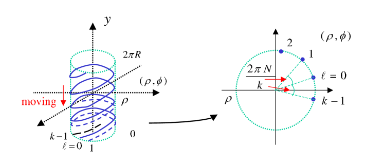
Figure 2: $(N,k)$ D-helix from k segments of spiral D1-branes

Then we can construct the boundary state for the $(N,k)$ D-helix (denoted as $|N,k\rangle$) by superposing k boundary states for properly shifted spiral D1-branes. That is

$$|N,k\rangle=\sum_{\ell=0}^{k-1}|N,k;\ell\rangle,\quad|N,k;\ell\rangle\equiv e^{-\frac{i}{2\pi\alpha^{\prime}}\int_{0}^{2\pi}d\sigma V_{N,k;\ell}}|D1\rangle,$$ (2.33)

where we defined the deformation operator $V_{N,k;\ell}$ as follows

$$V_{N,k;\ell}\equiv\rho\cos\Big{(}\frac{NX^{+}}{kR}+2\pi\frac{N\ell}{k}\Big{)}\partial_{\tau}X^{1}+\rho\sin\Big{(}\frac{NX^{+}}{kR}+2\pi\frac{N\ell}{k}\Big{)}\partial_{\tau}X^{2}.$$ (2.34)

We can interpret one segment as a ‘fractional’ brane and the $(N,k)$ D-helix as a ‘bulk’ brane in an orbifold theory . This is because we can obtain a $(N,k)$ D-helix from a $(N,1)$ D-helix in the space whose the radius in the $y$ direction is $kR$ via ${\mathbb{Z}}_{k}$ orbifolding. In the context of the orbifold theory, we can understand only one segment or any D-branes which are not periodic with $X^{+}\rightarrow X^{+}+2\pi R$ are inconsistent because these are not invariant under the ${\mathbb{Z}}_{k}$ symmetry.

Now let us compute the vacuum amplitude. Although we can easily calculate it in the same way as appeared in the previous section, the obtained result is not simple this time since the deformation operator $V_{N,k;\ell}$ is not periodic with $X^{+}\rightarrow X^{+}+2\pi R$ any longer. Anyway we find the following amplitude for $(N,k)$ D-helix

$${\cal A}(s)=\frac{{\cal N}}{(2\pi\alpha^{\prime}s)^{12}}\sum_{\ell,\ell^{\prime}=0}^{k-1}\sum_{w=-\infty}^{\infty}\exp\Big{[}-\sum_{m=1}^{\infty}L^{(\ell,\ell^{\prime})}_{m,w}(s)\Big{]}e^{-\frac{R^{2}w^{2}s}{2\alpha^{\prime}}}\eta^{-24}(is/\pi),$$ (2.35)

where the non trivial factor for the amplitude between $|N,k;\ell\rangle$ and $|N,k;\ell^{\prime}\rangle$ is given by

$$L^{(\ell,\ell^{\prime})}_{m,w}(s)=\frac{2\rho^{2}}{\pi^{2}\alpha^{\prime}}\frac{(m^{2}+(\frac{Nw}{k})^{2})}{(m^{2}-(\frac{Nw}{k})^{2})^{2}}\sin^{2}\Big{(}\frac{\pi Nw}{k}\Big{)}\frac{m}{e^{2ms}-1}\Big{[}e^{2ms}+1-2e^{ms}\cos\Big{(}\frac{2\pi N}{k}(\ell-\ell^{\prime})\Big{)}\Big{]}.$$ (2.36)

This amplitude reduces to eq.(2.15) in the limit of $k\rightarrow 1$ as expected. After taking a T-duality in the $y$ direction, we obtain the desired amplitude for the $(N,k)$ supertube.

Especially, we are interested in the large radius limit $\tilde{R}\rightarrow\infty$ of this amplitude. To keep the D0 charge density finite, we need to take the following limit

$$k\rightarrow\infty,\quad\frac{\tilde{R}}{\alpha^{\prime 1/2}}\rightarrow\infty,\quad\mbox{with}\quad b=\frac{\alpha^{\prime}}{\tilde{R}}\frac{k}{N}:\mbox{fixed}.$$ (2.37)

Notice that this corresponds to the deconstruction limit of the ${\mathbb{Z}}_{k}$ orbifold [43] (see the right picture of fig.2). In this limit, we can express the vacuum amplitude for the $(N,k)$ supertube as follows

$${\cal A}(s)=k^{2}{\cal N}_{0}\int_{0}^{1}dx\int_{-\infty}^{\infty}dp\frac{1}{(2\pi\alpha^{\prime}s)^{12}}\exp\Big{[}-\sum_{m=1}^{\infty}L_{m}(p,x,s)\Big{]}e^{-\frac{R^{2}w^{2}s}{2\alpha^{\prime}}}\eta^{-24}(is/\pi),$$ (2.38)

where we defined ${\cal N}_{0}$ as a usual normalization factor for D0-brane, i.e., ${\cal N}_{0}=\frac{\alpha^{\prime}T_{0}^{2}}{8}V_{0}$ and the non trivial exponential factor is given by

$$L_{m}(p,x,s)=\frac{2\rho^{2}}{\pi^{2}\alpha^{\prime}}\frac{m^{2}+(\frac{\alpha^{\prime}p}{b})^{2}}{\big{(}m^{2}-(\frac{\alpha^{\prime}p}{b})^{2}\big{)}^{2}}\sin^{2}(\frac{\pi\alpha^{\prime}p}{b})\frac{m}{e^{2ms}-1}(e^{2ms}+1-2e^{ms}\cos(2\pi Nx)).$$ (2.39)

Although it seems to be difficult to rewrite this amplitude in the language of the open string channel because we can not use the technique as in eq.(2.21), it will be interesting to compare above results with the matrix description of D-particles [2].

2.5 Generalization

As is claimed in [28], we can deform supertubes preserving 8 supersymmetries. Although the shapes of the sections of a tube in the constant $\tilde{y}$ plane have to be the same for any $\tilde{y}$, any shapes of section are OK (see the left picture in fig.3). Making T-duality in the $\tilde{y}$ direction, we obtain from a deformed $(N,k)$ supertube a deformed moving $(N,k)$ D-helix wrapped on the surface of the deformed supertube as claimed in [30] (see fig.3). In this T-dual picture, we can easily understand the validity of this deformation from the point of view of null deformation.

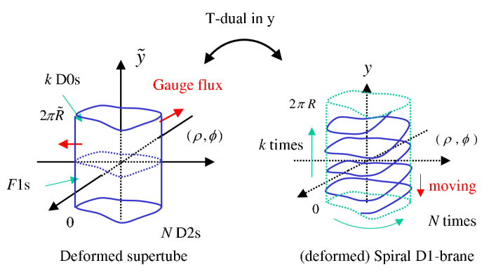
Figure 3: Deformed supertube and deformed D-helix

Therefore when the section with the plane $\tilde{y}=\mbox{const.}$ has the following form

$$X^{1}=\rho(\phi)\cos\phi,X^{2}=\rho(\phi)\sin\phi,$$ (2.40)

we can construct the boundary state for the deformed $(N,k)$ D-helix, the T-dual object of the deformed $(N,k)$ supertube, by using the following deformation operator instead of eq.(2.34)

$$\begin{split}V_{N,k;\ell}\equiv\,\,&\rho\Big{(}\frac{NX^{+}}{kR}+2\pi\frac{N\ell}{k}\Big{)}\cos\Big{(}\frac{NX^{+}}{kR}+2\pi\frac{N\ell}{k}\Big{)}\partial_{\tau}X^{1}\\ &+\rho\Big{(}\frac{NX^{+}}{kR}+2\pi\frac{N\ell}{k}\Big{)}\sin\Big{(}\frac{NX^{+}}{kR}+2\pi\frac{N\ell}{k}\Big{)}\partial_{\tau}X^{2}.\end{split}$$ (2.41)

In the same way as before, we can obtain exact vacuum amplitudes for deformed supertubes in the closed string channel, which vanish in the superstring case as expected from the point of view of the supersymmetry. Especially we can get the exact open string spectrum for deformed $(N,1)$ supertubes using the same technique as in eq.(2.21).

3 Supertube in Type IIA Gödel Universe

In this section we would like to consider supertubes on the type IIA Gödel universe [15], which is the T-dual of the type IIB PP-wave background with the maximal supersymmetry [25], in order to use them as probes of closed timelike curves. The supertubes correspond to moving D-helices, null deformed D1-branes, in the PP-wave via T-duality as in the case of the flat spacetime. As claimed in [27], the null deformed D-branes satisfy equation of motions also in the case of this PP-wave. We will find that we can construct the boundary states for supertubes in the universe in the same way as in the flat spacetime.

3.1 Relation between the Gödel Universe and PP-Wave

In this section we would like to give a brief review of the relation between the type IIA Gödel universe and the maximally supersymmetric type IIB PP-wave background. The type IIA Gödel universe has the following metric

$$ds^{2}=-(dt+\beta\sum_{i,j=1}^{8}J_{ij}x^{i}dx^{j})^{2}+\sum_{i=1}^{8}(dx^{i})^{2}+d\tilde{y}^{2},\quad J_{2k-1,2k}=s_{k}=\pm 1,$$ (3.1)

and NS-NS and RR 4-form flux

$$H_{2k-1,2k,\tilde{y}}=-2s_{k}\beta,\quad F_{1234}=F_{5678}=4\beta.$$ (3.2)

We will use the complex coordinates $z^{k}$ and the polar coordinates $(\rho_{k},\phi_{k})$ defined as

$$z^{k}=\rho_{k}e^{i\phi_{k}}\equiv x^{2k-1}+is_{k}x^{2k}.$$ (3.3)

This background has the closed time like curves for $\rho_{k}>1/\beta$.

On the other hand, the type IIB maximally supersymmetric PP-wave background is given by

$$\begin{split}ds^{2}=-2dx^{+}dx^{-}-\beta^{2}\sum_{i=1}^{8}(\tilde{x}^{i})^{2}(dx^{+})^{2}+\sum_{i=1}^{8}(d\tilde{x}^{i})^{2},\\ F_{(5)}=4\beta dx^{+}(d\tilde{x}^{1}d\tilde{x}^{2}d\tilde{x}^{3}d\tilde{x}^{4}+d\tilde{x}^{5}d\tilde{x}^{6}d\tilde{x}^{7}d\tilde{x}^{8}),\end{split}$$ (3.4)

where we defined the light cone directions as $x^{+}=t+y$, $x^{-}=(t-y)/2$ as before. The coordinate transformation

$$\tilde{x}^{2k-1}+is_{k}\tilde{x}^{2k}=(x^{2k-1}+is_{k}x^{2k})e^{-i\beta x^{+}}$$ (3.5)

changes this background into the following one

$$ds^{2}=-dt^{2}+dy^{2}+\sum_{i}(dx^{i})^{2}-2\beta\sum_{ij}J_{ij}x^{i}dx^{j}(dt+dy).$$ (3.6)

In this article we will call this background ‘the twisted PP-wave background’. Taking T-duality in $y$ direction, we obtain the Gödel universe (3.1),(3.2).

The twisted PP-wave background has the following symmetry (the translation in $x^{i}$) that leaves the metric and the flux unchanged

$$z^{k}\rightarrow z^{k}-\rho_{0k}e^{i\phi_{0k}},\quad x^{-}\rightarrow x^{-}+\sum_{k=1}^{4}\beta\rho_{0k}\rho_{k}\sin(\phi_{k}-\phi_{0k}).$$ (3.7)

This symmetry is equivalent to that for the PP-wave background (3.4) discussed in [27]. In this paper we would like to consider only the case of $s_{k}=(1,1,1,-1)$ because the Gödel universe has 20 supersymmetries in this case.

3.2 Supertube on the Gödel universe

Now let us consider the supertube extended in $(t,\phi_{1},\tilde{y})$ in the type IIA Gödel universe. As in the case of the flat spacetime, the analysis of the DBI action shows a supertube with the gauge flux $F_{t\tilde{y}}=-1$ and $F_{\phi_{1}\tilde{y}}=\mbox{constant}$ is a stable object. In order to take the T-duality in the $\tilde{y}$ direction, let us compactify the $\tilde{y}$ direction with the radius $\tilde{R}$. As in the case of the flat spacetime, the magnetic flux and the radius of the supertube $\rho$ are quantized as follows

$$F_{\phi_{1}\tilde{y}}=\frac{\alpha^{\prime}}{\tilde{R}}\frac{k}{N},\quad\rho^{2}=\frac{g_{s}\alpha^{\prime\frac{1}{2}}}{N}\left|\frac{qF_{\phi_{1}\tilde{y}}}{1-F_{\phi_{1}\tilde{y}}\beta}\right|,$$ (3.8)

where $N,k$ and $q$ are the numbers of D2-branes, D0-branes and F-strings respectively. In this paper we would like to treat only the case of $F_{\phi_{1}\tilde{y}}\beta<1$ because the tension of the supertube is the same as the sum of the tension of $|k|$ D0-branes and $|q|$ F-strings only in the case .

We can also show that the T-dual of this supertube is a moving spiral D1-brane as before. We can express the supertube as the following boundary conditions of open strings

$$\begin{split}\mu=t:&\quad-\partial_{N}t-\beta\rho^{2}\partial_{N}\phi-\partial_{D}\tilde{y}=0,\\ \mu=\phi:&\quad-\beta\rho^{2}\partial_{N}t+(\rho^{2}-\beta^{2}\rho^{4})\partial_{N}\phi+(b-\beta\rho^{2})\partial_{D}\tilde{y}=0,\\ \mu=\tilde{y}:&\quad\partial_{N}\tilde{y}+\partial_{D}t+(\beta\rho^{2}-b)\partial_{D}\phi=0,\\ \mu=\rho:&\ \quad\partial_{D}\rho=0,\end{split}$$ (3.9)

where we defined $F_{\phi\tilde{y}}=b$. Taking the T-duality in $\tilde{y}$ direction, these change to

$$\partial_{N}x^{+}=0,\quad\partial_{N}x^{-}+(\beta-\frac{1}{b})\rho^{2}\partial_{N}\phi=0,\quad\partial_{D}(\phi-\frac{1}{b}x^{+})=0,\quad\partial_{D}\rho=0,$$ (3.10)

where we used the following relations of the T-duality (see [16] in detail)

$$\partial_{N}\tilde{y}=\partial_{D}y-\beta\rho^{2}\partial_{D}\phi,\quad\partial_{D}\tilde{y}=\partial_{N}y-\beta\rho^{2}\partial_{N}\phi.$$ (3.11)

After the translation (3.7), we find that eq.(3.10) is just the condition of the moving spiral D1-brane in the twisted PP-wave background.

3.3 String Theory on the Twisted PP-wave Background

In the previous section we have found that as in the case of the flat spacetime, the T-dual of the supertube in the type IIA Gödel universe is a moving spiral D1-brane in the twisted PP-wave background. Before constructing the boundary state for this spiral D1-brane, let us review the string theory on the twisted PP-wave background (3.6) (see [16] in detail). As expected from the name of the background, this is just the twisted version of the string theory on the type IIB maximally supersymmetric PP-wave background [26]. In this section we will treat only the bosonic part because the (GS) fermionic part is irrelevant to our analysis. We will review closed strings first, consider open strings on the static D1-brane extended in $t$ and $y$ directions next and finally study the open closed duality of this D1-brane.

Closed String Theory

Now let us consider the closed string theory on the twisted PP-wave. Since the $y$ direction is compactified with the radius $R=\alpha^{\prime}/\tilde{R}$, we should impose the light cone gauge $X^{+}=\alpha^{\prime}p^{+}\tau+wR\sigma$. In this gauge, the (light cone) closed string action is given by

$$S_{closed}=-\frac{1}{2\alpha^{\prime}}\int d\tau\int_{0}^{2\pi}d\sigma[\partial_{a}X^{i}\partial^{a}X^{i}+2\beta X^{i}J_{ij}(p^{+}\partial_{\tau}X^{j}-wR\partial_{\sigma}X^{j})],$$ (3.12)

where we set the world sheet metric at $\eta^{ab}=\mbox{diag}(-1,1)$. After rewriting this action with the complex coordinates $Z^{k}$ in eq.(3.3) and defining $Z^{k}_{0}$ as $Z^{k}=e^{i\beta s_{k}X^{+}}Z^{k}_{0}$, we find that the equation of motion of $Z^{k}_{0}$ is just that of the type IIB maximally supersymmetric PP-wave background. That is

$$(\partial_{\tau}^{2}-\partial_{\sigma}^{2})Z^{k}_{0}+f^{2}Z^{k}_{0}=0,\quad f^{2}=(\beta\alpha^{\prime}p^{+})^{2}-(\beta Rw)^{2}.$$ (3.13)

Noticing that closed strings should satisfy the following twisted boundary condition

$$Z^{k}_{0}(\tau,\sigma+2\pi)=e^{-2\pi i\delta}Z^{k}_{0}(\tau,\sigma),\quad\delta=s_{k}\beta Rw,$$ (3.14)

we find the mode expansions of $Z^{k}_{0}$ and $\bar{Z}^{k}_{0}$, the complex conjugate of $Z^{k}_{0}$, are given by

$$\begin{split}Z^{k}_{0}&=i\sqrt{\frac{\alpha^{\prime}}{2}}\sum_{n\in{\mathbb{Z}}}\Big{(}\frac{\alpha^{k}_{n+\delta}}{w^{+}_{n}}e^{-iw^{+}_{n}\tau-i(n+\delta)\sigma}+\frac{\tilde{\alpha}^{k}_{n-\delta}}{w^{-}_{n}}e^{-iw^{-}_{n}\tau+i(n-\delta)\sigma}\Big{)},\\ \bar{Z}^{k}_{0}&=i\sqrt{\frac{\alpha^{\prime}}{2}}\sum_{n\in{\mathbb{Z}}}\Big{(}\frac{\bar{\alpha}^{k}_{n-\delta}}{w^{-}_{n}}e^{-iw^{-}_{n}\tau-i(n-\delta)\sigma}+\frac{\bar{\tilde{\alpha}}^{k}_{n+\delta}}{w^{+}_{n}}e^{-iw^{+}_{n}\tau+i(n+\delta)\sigma}\Big{)},\end{split}$$ (3.15)

where we defined

$$\begin{split}&w^{+}_{n}=\left\{\begin{array}[]{ll}\sqrt{(n+\delta)^{2}+f^{2}}&\mbox{for}\quad n\geq-\delta\\ -\sqrt{(n+\delta)^{2}+f^{2}}&\mbox{for}\quad n<-\delta\end{array}\right.,\\ &w^{-}_{n}=\left\{\begin{array}[]{ll}\sqrt{(n-\delta)^{2}+f^{2}}&\mbox{for}\quad n>\delta\\ -\sqrt{(n-\delta)^{2}+f^{2}}&\mbox{for}\quad n\leq\delta\end{array}\right..\end{split}$$ (3.16)

Oscillators satisfy the following quantization condition

$$[\alpha^{k}_{n+\delta},\bar{\alpha}^{k^{\prime}}_{\ell-\delta}]=2w^{+}_{n}\delta_{\ell+n,0}\delta_{kk^{\prime}},\quad[\tilde{\alpha}^{k}_{n-\delta},\bar{\tilde{\alpha}}^{k^{\prime}}_{\ell+\delta}]=2w^{-}_{n}\delta_{n+\ell,0}\delta_{kk^{\prime}}.$$ (3.17)

The closed string Hamiltonian is expressed as follows

$${\cal H}_{c}=\frac{R^{2}w^{2}}{2\alpha^{\prime}}-\alpha^{\prime}p^{+}p^{-}+H_{c}.$$ (3.18)

The massive mode $H_{c}$ is given by

$$H_{c}=\sum_{k=1}^{4}\sum_{n\in{\mathbb{Z}}}\Big{[}N^{k+}_{n}(\sqrt{(n+\delta)^{2}+f^{2}}+\beta\alpha^{\prime}p^{+})+N^{k-}_{n}(\sqrt{(n-\delta)^{2}+f^{2}}-\beta\alpha^{\prime}p^{+})\Big{]}+8\Delta(f;\delta),$$ (3.19)

where $\Delta(f;\delta)$ is the zero point energy (see eq.(A.2)) and we defined the number operators as

$$\begin{split}&N^{k+}_{n}=\left\{\begin{array}[]{ll}\frac{1}{2w^{+}_{n}}\tilde{\alpha}^{k}_{-n-\delta}\tilde{\bar{\alpha}}^{k}_{n+\delta}&\mbox{for}\quad n\geq-\delta\\ \frac{1}{2w^{-}_{-n}}\alpha^{k}_{n+\delta}{\bar{\alpha}}^{k}_{-n-\delta}&\mbox{for}\quad n<-\delta\end{array}\right.,\\ &N^{k-}_{n}=\left\{\begin{array}[]{ll}\frac{1}{2w^{-}_{n}}\tilde{\bar{\alpha}}^{k}_{-n+\delta}\tilde{\alpha}^{k}_{n-\delta}&\mbox{for}\quad n>\delta\\ \frac{1}{2w^{+}_{-n}}\bar{\alpha}^{k}_{n-\delta}\alpha^{k}_{-n+\delta}&\mbox{for}\quad n\leq\delta\end{array}\right..\end{split}$$ (3.20)

Notice that the zero point energy in (3.19) is canceled by the fermionic one due to the supersymmetry .

Finally we would like to comment on the case of $p^{+}=0$. We need to consider the case because in the closed string channel, the Neumann boundary condition in the $x^{+}$ direction is expressed as $\partial_{\tau}X^{+}=0$. In this case, we should modify the $n=0$ sector in eq.(3.15) into the complex momenta and positions, i.e.,

$$Z^{k}_{0}=(\alpha^{\prime}p^{k}_{z}\tau+z^{k})e^{-i\delta\sigma}+\cdots,\quad\bar{Z}^{k}_{0}=(\alpha^{\prime}\bar{p}^{k}_{z}\tau+\bar{z}^{k})e^{i\delta\sigma}+\cdots,\quad[z^{k},\bar{p}^{k^{\prime}}_{z}]=2i\delta_{kk^{\prime}}.$$ (3.21)

Open Strings on D1-brane

Next let us consider open strings on the D1-brane extended in the light cone directions in the twisted PP-wave background. We have only to consider the D1-brane at $Z^{k}=0$, because the background is homogeneous one. We can obtain the open string spectrum from the closed string one using the doubling trick. We need to set $\delta=0$ in eq.(3.15) because the light cone gauge for the open strings on this D1-brane is $X^{+}=2\alpha^{\prime}p^{+}\tau$. Noticing that the boundary condition $Z^{k}=0$ at $\sigma=0$ and $\pi$ is equivalent to the following gluing condition

$$\alpha^{k}_{n}=-\tilde{\alpha}^{k}_{n}\quad\mbox{for}\quad n\neq 0,\quad\alpha^{k}_{0}=\tilde{\alpha}^{k}_{0}=0,$$ (3.22)

we obtain the mode expansion of the open string on the D1-brane as follows

$$Z^{k}_{0}=\sqrt{2\alpha^{\prime}}\sum_{n\neq 0}\frac{\alpha^{k}_{n}}{w_{n}}\sin(n\sigma)e^{-iw_{n}\tau},\quad w_{n}\equiv\mbox{sgn}(n)\sqrt{n^{2}+m^{2}},\quad m\equiv 2\beta\alpha^{\prime}p^{+}.$$ (3.23)

The commutation relations are $[\alpha^{k}_{n},\alpha^{k^{\prime}}_{\ell}]=2w_{n}\delta_{\ell+n,0}\delta^{kk^{\prime}}$. The mode expansion of $\bar{Z}^{k}_{0}$ is just the complex conjugate of $Z^{k}_{0}$. The open string Hamiltonian is expressed as follows

$${\cal H}_{o}=-2\alpha^{\prime}p^{+}p^{-}+H_{o}.$$ (3.24)

The massive mode $H_{o}$ is given by

$$H_{o}=\sum_{n=1}^{\infty}\Big{[}N^{+}_{n}(\sqrt{n^{2}+m^{2}}+m)+N^{-}_{n}(\sqrt{n^{2}+m^{2}}-m)\Big{]}+4\Delta(m;0)-2|m|,$$ (3.25)

where we defined the number operators as follows

$$N^{+}_{n}=\sum_{k=1}^{4}\frac{1}{2w_{n}}\alpha^{k}_{-n}{\bar{\alpha}}^{k}_{n},\quad N^{-}_{n}=\sum_{k=1}^{4}\frac{1}{2w_{n}}{\bar{\alpha}}^{k}_{-n}\alpha^{k}_{n}.$$ (3.26)

The zero point energy $4\Delta(m;0)-2|m|$ is canceled by the fermionic one due to the supersymmetry as in the case of closed strings . Finally let us compute the following open string vacuum amplitude

$$Z^{k}_{open}=\int_{0}^{\infty}\frac{dt}{t}\int dp^{+}dp^{-}\mbox{Tr}\exp[-2\pi t(-2\alpha^{\prime}p^{+}p^{-}+H_{o})].$$ (3.27)

When we define $q=e^{-2\pi t}$ as before, we find the non-trivial part is given by

$$\mbox{Tr}e^{-2\pi tH_{o}}=\left[q^{\Delta(m;0)-\frac{|m|}{2}}\prod_{p=1}^{\infty}\frac{1}{(1-q^{\sqrt{p^{2}+m^{2}}+m})(1-q^{\sqrt{p^{2}+m^{2}}-m})}\right]^{4}\equiv f(q,m)^{4}.$$ (3.28)

Open Closed Duality of D1-brane

In the rest of this section, we would like to study the open closed duality of D1-brane in the twisted PP-wave background. Noticing that the relation between the mass parameter of the open strings $m$ and that of the closed strings $\delta$ is $mt=-i\delta$ (see eq.(2.21)), we obtain the following modular transformation rule

$$\begin{split}f(q,m)=\sqrt{\frac{2\pi^{3}\alpha^{{}^{\prime}2}\sin(2\pi\delta)}{\delta}}\frac{\tilde{q}^{\Delta(i\delta;\delta)}}{(2\pi\alpha^{\prime}s)}\prod_{n\neq 0}\frac{1}{1-\tilde{q}^{\sqrt{(n+\delta)^{2}-\delta^{2}}}}\equiv\tilde{f}(\tilde{q},\delta),\quad\tilde{q}=e^{-2s},\end{split}$$ (3.29)

where we used the modular properties of the massive theta functions in the PP-wave background. Therefore the Cardy’s condition is given by (see eq.(2.22))

$$\langle D1,w|e^{-sH_{c}}|D1,w\rangle=\tilde{f}(\tilde{q},\delta_{w})^{4},\quad\delta_{w}\equiv\beta Rw,$$ (3.31)

where $|D1,w\rangle$ denotes the boundary state for D1-brane with the winding $w$ sector. We can construct the boundary state for the D1-brane satisfying this condition. The result is

$$|D1,w\rangle=\left(\frac{2\pi^{3}\alpha^{{}^{\prime}2}\sin(2\pi\delta_{w})}{\delta_{w}}\right)\int\frac{dp_{z}^{k}d\bar{p}_{z}^{k}}{(2\pi)^{8}}|w\rangle\!\rangle\otimes|p_{z}^{k},\bar{p}^{k}_{z}\rangle,$$ (3.32)

where $|w\rangle\!\rangle$ is the following Ishibashi state for the D1-brane

$$|w\rangle\!\rangle\equiv\exp\Big{[}\sum_{\begin{subarray}{c}n>\delta_{w}\\ n\neq 0\end{subarray}}\frac{1}{2w_{n}^{+}}\bar{\tilde{\alpha}}^{k}_{-n+\delta_{w}}\alpha^{k}_{-n+\delta_{w}}+\sum_{\begin{subarray}{c}n>-\delta_{w}\\ n\neq 0\end{subarray}}\frac{1}{2w_{n}^{-}}{\tilde{\alpha}}^{k}_{-n-\delta_{w}}\bar{\alpha}^{k}_{-n-\delta_{w}}\Big{]}|0\rangle.$$ (3.33)

3.4 Boundary State for the Supertube on Gödel Universe

In the previous section we have reviewed the string theory on the twisted PP-wave background which is the T-dual of the type IIA Gödel universe. We have also constructed the boundary state for the D1-brane at $Z^{k}=0$ in the twisted PP-wave background.

We now would like to construct the boundary state for a moving spiral D1-brane in the twisted PP-wave background using the null deformations as in the case of the flat spacetime. This spiral D1-brane corresponds to a supertube in the Gödel universe. In this section we will consider only the case of $k=1$ for simplicity.

As in the case of the flat spacetime, let us consider the following boundary state without light gauge fixing

$$|N,1\rangle=e^{-\frac{i}{2\pi\alpha^{\prime}}\int_{0}^{2\pi}d\sigma[\rho\cos(\frac{Nx^{+}}{R})P_{1}+\rho\sin(\frac{Nx^{+}}{R})P_{2}]}|D1\rangle,$$ (3.34)

where $P_{\mu}\equiv G_{\mu\lambda}\partial_{\tau}X^{\lambda}$ is the canonical momentum of the world sheet theory on the twisted PP-wave background (3.6). We can also replace $P_{i}$ with $\partial_{\tau}X^{i}$ in eq.(3.34) noticing the Neumann condition $\partial_{\tau}X^{+}|D1\rangle=0$. Formally we can show that the above boundary state satisfies boundary conditions for the $(N,1)$ D-helix (3.10) and the boundary conformal invariance by using the canonical quantization $[P_{\mu}(\sigma,\tau),X^{\nu}(\sigma^{\prime},\tau)]=-i\delta_{\mu}^{\nu}\delta(\sigma-\sigma^{\prime})$. However we should take a great care since the naive expression (3.34) would be divergent. We can avoid the divergence by renormalization, however it breaks the boundary conformal invariance in general.

Fortunately in the case of the twisted PP-wave background, the canonical quantization condition indicates that the operator products $X^{+}X^{+}$ and $X^{+}X^{i}$ have no singular terms. As in [5], this implies that the deformation operator is exactly marginal . Therefore the boundary state (3.34) is that for the $(N,1)$ D-helix up to a normalization factor. The normalization factor is determined by the Cardy’s condition and we will find later that no extra normalization factor is needed as in the case of the flat spacetime. The same argument shows that we can construct the boundary states for null deformed D-branes on the twisted PP-wave background by multiplying those for static D1-branes by the Wilson line like operators . Notice that deformations with respect to $X^{-}$ are not allowed as expected because the operator product $X^{-}X^{i}$ will have singular terms.

Now in the light cone gauge $X^{+}=Rw\sigma$, eq.(3.34) is expressed as the following form

$$|N,1\rangle=e^{-\frac{i}{2\pi\alpha^{\prime}}\int_{0}^{2\pi}d\sigma V_{N,1}}|D1\rangle,\quad V_{N,1}=\frac{\rho}{2}[e^{-iNw\sigma}\partial_{\tau}Z^{1}+e^{iNw\sigma}\partial_{\tau}\bar{Z}^{1}].$$ (3.36)

We can compute the vacuum amplitude between the same D-helix in the same way as in the case of the flat spacetime. The result is given by

$${\cal A}(s)=\sum_{w}\exp\Big{[}-\frac{\rho^{2}}{\alpha^{\prime}}w_{-Nw}\tanh\left(\frac{sw_{-Nw}}{2}\right)\Big{]}e^{-\frac{R^{2}w^{2}s}{2\alpha^{\prime}}}\tilde{f}(\tilde{q},\delta_{w})^{4},$$ (3.37)

where we defined

$$w^{2}_{-Nw}=(\beta wR)^{2}\Big{[}(-\frac{N}{\beta R}+1)^{2}-1\Big{]}=(wR)^{2}\Big{(}\frac{1-2b\beta}{b^{2}}\Big{)}.$$ (3.38)

In the final line we used the relation $b=\frac{R}{N}$. Notice that $w_{-Nw}$ becomes pure imaginary for $2b\beta>1$ After taking the T-duality in the $y$ direction $(R\rightarrow\alpha^{\prime}/\tilde{R})$, we obtain the vacuum amplitude of the $(N,1)$ supertube.

Let us consider the naive $s\rightarrow 0$ limit, the UV limit of closed strings. In this limit, the non-trivial factor in eq.(3.37) can be interpreted as the following radius shift

$$\exp\Big{[}-\frac{R^{2}w^{2}s}{2\alpha^{\prime}}-\frac{\rho^{2}w^{2}_{-Nw}s}{2\alpha^{\prime}}\Big{]}=\exp\Big{[}-\frac{R^{{}^{\prime}2}w^{2}s}{2\alpha^{\prime}}\Big{]},$$ (3.39)

where the shifted radius $R^{\prime}$ is given by

$$R^{{}^{\prime}2}=R^{2}\Big{[}1+\frac{\rho^{2}}{b^{2}}(1-2b\beta)\Big{]}.$$ (3.40)

For $2b\beta>1$, the square of shifted radius becomes negative when $\rho^{2}>\frac{b^{2}}{2b\beta-1}$. Therefore one might think this is the tachyonic instability of closed strings wound in y direction (or closed strings with the nonzero momentum $p_{y}$ in the Gödel universe). However we should interpret the region $s\sim 0$ as the open string IR rather than the closed string UV. Notice that the naive $s\rightarrow 0$ limit is different from the IR limit of open strings because the conformal invariance of the world sheet theory is broken by the gauge fixing, i.e., the mass parameter is changed under the open closed duality.

3.5 Open String Spectrum on Supertube in Gödel Universe

As we have found in the previous section, we have to treat the vacuum amplitude in the open string picture to carry out the correct physical interpretations. In this section we would like to rewrite the obtained vacuum amplitude in the language of the open string channel using the same method as before. As in the case of the flat spacetime, we will compare the result to the following open string metric of the supertube in Gödel universe

$$G^{tt}_{eff}=-\left(1+\rho^{2}\frac{(1-2b\beta)}{b^{2}}\right).$$ (3.41)

Especially, we are interested in the case of $2b\beta>1$ because the effective metric $G^{tt}_{eff}$ changes its sign for large values of $\rho$ in the case . This is the signal of the closed timelike curves in the Gödel universe. Therefore we will consider only the case of $2b\beta>1$ below.

Using the correspondence $2i\alpha^{\prime}p^{+}t\leftrightarrow wR$, we can rewrite the non trivial part in eq.(3.37) in the language of the open string channel as follows

$$-\frac{\rho^{2}}{\alpha^{\prime}}w_{Nw}\tanh\frac{w_{Nw}s}{2}\rightarrow-2\pi t\Big{[}\frac{\rho^{2}p^{+}}{\pi}\sqrt{\frac{2b\beta-1}{b^{2}}}\tanh\Big{(}\pi\alpha^{\prime}p^{+}\sqrt{\frac{2b\beta-1}{b^{2}}}\Big{)}\Big{]}.$$ (3.42)

Then we obtain the following open string Hamiltonian of the $(N,1)$ D-helix

$${\cal H}_{o}=-2\alpha^{\prime}p^{+}p^{-}+\frac{\rho^{2}p^{+}}{\pi}\sqrt{\frac{2b\beta-1}{b^{2}}}\tanh\Big{(}\pi\alpha^{\prime}p^{+}\sqrt{\frac{2b\beta-1}{b^{2}}}\Big{)}+H_{o}.$$ (3.43)

Notice that the open-closed duality (3.42) shows that no extra normalization factor in the boundary state (3.34) is needed as we promised. After taking T-duality in y direction, we obtain the open string Hamiltonian on the $(N,1)$ supertube on the Gödel universe. For open strings with no windings in the $\tilde{y}$ direction, the result is given by

$${\cal H}_{o}=-\alpha^{\prime}E^{2}+\frac{\rho^{2}E}{\pi}\sqrt{\frac{2b\beta-1}{b^{2}}}\tanh\Big{(}\pi\alpha^{\prime}E\sqrt{\frac{2b\beta-1}{b^{2}}}\Big{)}+H_{o},$$ (3.44)

where the massive mode $H_{o}$ is given by

$$H_{o}=\sum_{n=1}^{\infty}\Big{[}N^{+}_{n}(\sqrt{n^{2}+(2\beta\alpha^{\prime}E)^{2}}+2\beta\alpha^{\prime}E)+N^{-}_{n}(\sqrt{n^{2}+(2\beta\alpha^{\prime}E)^{2}}-2\beta\alpha^{\prime}E)\Big{]}.$$ (3.45)

Remember that we can neglect the zero point energy due to the supersymmetry. In the low energy limit $|\alpha^{\prime}E\sqrt{\frac{2b\beta-1}{b^{2}}}|\ll 1$, we can read off the open string metric (3.41) from the Hamiltonian (3.44) as expected.

Now let us consider the open string spectrum ${\cal H}_{0}=0$. If there were no $\alpha^{\prime}$ correction in eq.(3.44), this would have the form $-\alpha^{\prime}G^{tt}_{eff}E^{2}=H_{o}$. Therefore we can interpret the effect of the closed timelike curve as the tachyonic instability of the open strings. That is, the energy $E$ becomes imaginary. However there is a non trivial $\alpha^{\prime}$ correction in eq.(3.44). Since the magnitude of $\tanh x$ is always smaller than that of $x$, this tachyonic instability becomes smaller at the string theory level than obtained from the low energy interpretation. Notice that we can indeed find the real $E$ satisfying ${\cal H}_{o}=0$ for any radius of the supertube $\rho$ . Therefore we can conclude that there is no tachyonic instability of open strings at the string theory level.

4 Conclusion

In this article we have constructed the boundary states for supertubes in the flat spacetime in the covariant formalism and read stringy information from the vacuum amplitude of open strings on the supertube. The supertube is the stable tubular D2-branes with the ‘critical’ electric flux and constant magnetic flux on them, i.e., the bound state of $N$ D2-branes, $k$ D0-branes and $q$ F-strings. Supertubes are also the BPS solitons preserving 8 supercharges. Taking the T-duality in the direction in which the supertube is extended, we obtain the moving spiral D1-brane (D-helix) wound $k$ times in the T-dual direction and $N$ times in the angular direction. We can also interpret this D-helix as the symmetrically placed $k$ segments of spiral D1-branes. Since adding the ‘critical’ electric flux corresponds to null boosting in the T-dual picture, we can obtain the D-helix from a static D1-brane via null deformation, the deformation only in the $x^{+}$ direction. This is consistent with the fact that any null deformed D-brane preserves 8 supercharges which is the same as the number of the supercharges of the supertube. This is the basic idea needed to construct the boundary states.

First we have constructed the boundary state for the $(N,k)$ D-helix from $k$ segments of D1-branes via null deformation in the covariant formalism. We have found that we can interpret one segment of the spiral D1-brane as a ‘fractional’ brane and the $(N,k)$ D-helix as a ‘bulk’ brane in an orbifold theory. We have also computed the vacuum amplitude of the open strings on the supertube in an exact form in the closed string channel. In the superstring case, we found the vacuum amplitude is zero as expected from the point of view of the supersymmetry.

In particular, we found the open string spectrum on the $k=1$ supertube in an exact form using the open closed duality in the discretized light cone gauge. This is due to the fact that the $k=1$ D-helix has the good periodicity in the light cone direction. In the low energy limit, we can read the open string metric from the open string spectrum. On the other hand we have found a non-trivial $\alpha^{\prime}$ correction in the high energy region. We found there is a ‘critical’ energy for open strings on the supertube due to this stringy correction.

It is known that we can deform the section of the supertube preserving 8 supercharges. We can easily understand this fact in the T-dual picture from the point of view of null deformation. We have also constructed the boundary states for these deformed supertubes in the same way. We can exactly calculate the vacuum amplitude which vanishes in the superstring case and find an exact open string spectrum in the case of $k=1$.

We have also considered supertubes in the supersymmetric type IIA Gödel universe in order to use them as probes of closed timelike curves. Since the T-dual of this universe is the type IIB PP-wave background with maximal supersymmetry where null deformation is allowed, we can construct the boundary states for supertubes in the same way as in the case of the flat spacetime. We calculated the vacuum amplitude for the $k=1$ supertube and found the open string spectrum. In the open string spectrum, the effect of the closed timelike curve appears as the tachyonic instability of open strings. We found this tachyonic instability disappears at the string theory level due to the non-trivial $\alpha^{\prime}$ correction of the spectrum.

Acknowledgments

The author would like to thank T. Eguchi, K. Hashimoto, Y. Hyakutake, K. Sakai, Y. Sugawara, T. Takayanagi and S. Yamaguchi for useful discussions and comments. The author is also grateful to Yukawa Institute for Theoretical Physics for hospitality during the completion of this paper.

Appendix A Massive Theta Functions

Here we would like to summarize the definition of the massive theta functions [44] and their modular properties. We define the massive theta functions as follows

$$\Theta_{(a,b)}(\tau;m)\equiv e^{4\pi\tau\Delta(m;a)}\prod_{n\in{\mathbb{Z}}}(1-e^{-2\pi\tau\sqrt{m^{2}+(n+a)^{2}}+2\pi ib})(1-e^{-2\pi\tau\sqrt{m^{2}+(n+a)^{2}}-2\pi ib}),$$ (A.1)

where the zero-point energy $\Delta(m;a)$ is given by

$$\begin{split}\Delta(m;a)&\equiv\frac{1}{2}\Big{(}\sum_{n\in{\mathbb{Z}}}\sqrt{m^{2}+(n+a)^{2}}-\int_{-\infty}^{\infty}dk\sqrt{m^{2}+k^{2}}\Big{)}\\ &=-\frac{1}{2\pi^{2}}\sum_{n=1}^{\infty}\int_{0}^{\infty}dse^{-sn^{2}-\frac{\pi^{2}m^{2}}{s}}\cos(2\pi na).\end{split}$$ (A.2)

These theta functions have the following modular property (see [45] in detail)

$$\Theta_{(a,b)}(1/t,mt)=\Theta_{(b,-a)}(t;m).$$ (A.3)

References

- [1] D. Mateos and P. K. Townsend, “Supertubes,” Phys. Rev. Lett. 87 (2001) 011602, hep-th/0103030.
- [2] D. Bak and K. M. Lee, “Noncommutative supersymmetric tubes,” Phys. Lett. B 509 (2001) 168, hep-th/0103148.
- [3] R. C. Myers, “Dielectric-branes,” JHEP 9912 (1999) 022, hep-th/9910053.
- [4] J. H. Cho and P. Oh, “Super D-helix,” Phys. Rev. D 64 (2001) 106010, hep-th/0105095.
- [5] C. G. Callan and I. R. Klebanov, “D-Brane Boundary State Dynamics,” Nucl. Phys. B 465 (1996) 473, hep-th/9511173.
- [6] C. Bachas and C. Hull, “Null brane intersections,” JHEP 0212 (2002) 035, hep-th/0210269.
- [7] R. C. Myers and D. J. Winters, “From D - anti-D pairs to branes in motion,” JHEP 0212 (2002) 061, hep-th/0211042.
- [8] C. Bachas, “Relativistic string in a pulse,” Annals Phys. 305 (2003) 286, hep-th/0212217.
- [9] B. Durin and B. Pioline, “Open strings in relativistic ion traps,” JHEP 0305 (2003) 035, hep-th/0302159.
- [10] Y. Hikida, H. Takayanagi and T. Takayanagi, “Boundary states for D-branes with traveling waves,” JHEP 0304 (2003) 032, hep-th/0303214.
- [11] M. R. Douglas and G. W. Moore, “D-branes, Quivers, and ALE Instantons,” hep-th/9603167.
- [12] K. Godel, “An Example Of A New Type Of Cosmological Solutions Of Einstein’s Field Equations Of Graviation,” Rev. Mod. Phys. 21 (1949) 447.
- [13] J. P. Gauntlett, J. B. Gutowski, C. M. Hull, S. Pakis and H. S. Reall, “All supersymmetric solutions of minimal supergravity in five dimensions,” hep-th/0209114.
- [14] C. A. Herdeiro, “Spinning deformations of the D1-D5 system and a geometric resolution of closed timelike curves,” Nucl. Phys. B 665 (2003) 189, hep-th/0212002.
- [15] E. K. Boyda, S. Ganguli, P. Horava and U. Varadarajan, “Holographic protection of chronology in universes of the Goedel type,” Phys. Rev. D 67 (2003) 106003, hep-th/0212087.
- [16] T. Harmark and T. Takayanagi, “Supersymmetric Goedel universes in string theory,” Nucl. Phys. B 662 (2003) 3, hep-th/0301206.
- [17] E. G. Gimon and A. Hashimoto, “Black holes in Goedel universes and pp-waves,” Phys. Rev. Lett. 91 (2003) 021601, hep-th/0304181.
- [18] N. Drukker, B. Fiol and J. Simon, “Goedel’s universe in a supertube shroud,” hep-th/0306057.
- [19] Y. Hikida and S. J. Rey, “Can branes travel beyond CTC horizon in Goedel universe?,” hep-th/0306148.
- [20] D. Brecher, P. A. DeBoer, D. C. Page and M. Rozali, “Closed timelike curves and holography in compact plane waves,” hep-th/0306190.
- [21] V. E. Hubeny, M. Rangamani and S. F. Ross, “Causal inheritance in plane wave quotients,” hep-th/0307257.
- [22] D. Brace, C. A. Herdeiro and S. Hirano, “Classical and quantum strings in compactified pp-waves and Goedel type universes,” hep-th/0307265.
- [23] D. Brace, “Closed Geodesics on Godel-type Backgrounds,” hep-th/0308098.
- [24] D. Brecher, U. H. Danielsson, J. P. Gregory and M. E. Olsson, “Rotating black holes in a Goedel universe,” hep-th/0309058.
- [25] M. Blau, J. Figueroa-O’Farrill, C. Hull and G. Papadopoulos, “A new maximally supersymmetric background of IIB superstring theory,” JHEP 0201 (2002) 047, hep-th/0110242.
- [26] R. R. Metsaev, “Type IIB Green-Schwarz superstring in plane wave Ramond-Ramond background,” Nucl. Phys. B 625 (2002) 70, hep-th/0112044.
- [27] K. Skenderis and M. Taylor, “Open strings in the plane wave background. I: Quantization and symmetries,” hep-th/0211011.
- [28] D. Mateos, S. Ng and P. K. Townsend, “Tachyons, supertubes and brane/anti-brane systems,” JHEP 0203 (2002) 016, hep-th/0112054.
- [29] D. Mateos, S. Ng and P. K. Townsend, “Supercurves,” Phys. Lett. B 538 (2002) 366, hep-th/0204062.
- [30] Y. Hyakutake and N. Ohta, “Supertubes and supercurves from M-ribbons,” Phys. Lett. B 539 (2002) 153, hep-th/0204161.
- [31] D. s. Bak and A. Karch, “Supersymmetric brane-antibrane configurations,” Nucl. Phys. B 626 (2002) 165, hep-th/0110039.
- [32] D. s. Bak and N. Ohta, “Supersymmetric D2 anti-D2 strings,” Phys. Lett. B 527 (2002) 131, hep-th/0112034.
- [33] D. s. Bak, N. Ohta and M. M. Sheikh-Jabbari, “Supersymmetric brane anti-brane systems: Matrix model description, stability and decoupling limits,” JHEP 0209 (2002) 048, hep-th/0205265.
- [34] C. G. Callan, C. Lovelace, C. R. Nappi and S. A. Yost, “Loop Corrections To Superstring Equations Of Motion,” Nucl. Phys. B 308 (1988) 221.
- [35] M. Kruczenski, R. C. Myers, A. W. Peet and D. J. Winters, “Aspects of supertubes,” JHEP 0205 (2002) 017, hep-th/0204103.
- [36] O. Bergman, M. R. Gaberdiel and M. B. Green, “D-brane interactions in type IIB plane-wave background,” JHEP 0303 (2003) 002, hep-th/0205183.
- [37] M. R. Gaberdiel and M. B. Green, “The D-instanton and other supersymmetric D-branes in IIB plane-wave string theory,” hep-th/0211122.
- [38] N. Seiberg and E. Witten, “String theory and noncommutative geometry,” JHEP 9909 (1999) 032, hep-th/9908142.
- [39] E. Dudas and J. Mourad, “D-branes in string theory Melvin backgrounds,” Nucl. Phys. B 622 (2002) 46, hep-th/0110186.
- [40] T. Takayanagi and T. Uesugi, “D-branes in Melvin background,” JHEP 0111 (2001) 036, hep-th/0110200.
- [41] H. Takayanagi and T. Takayanagi, “Open strings in exactly solvable model of curved space-time and pp-wave limit,” JHEP 0205 (2002) 012, hep-th/0204234].
- [42] J. G. Russo and A. A. Tseytlin, “Exactly solvable string models of curved space-time backgrounds,” Nucl. Phys. B 449 (1995) 91, hep-th/9502038.
- [43] N. Arkani-Hamed, A. G. Cohen and H. Georgi, “(De)constructing dimensions,” Phys. Rev. Lett. 86 (2001) 4757, hep-th/0104005.
- [44] T. Takayanagi, “Modular invariance of strings on pp-waves with RR-flux,” JHEP 0212 (2002) 022, hep-th/0206010.
- [45] Y. Sugawara, “Thermal amplitudes in DLCQ superstrings on pp-waves,” Nucl. Phys. B 650 (2003) 75, hep-th/0209145.