SISSA 76/2003/FM

Universal ratios along a line of critical points.
The Ashkin–Teller model
Gesualdo Delfino and Paolo Grinza

International School for Advanced Studies (SISSA)
via Beirut 2-4, 34014 Trieste, Italy
INFN sezione di Trieste
E-mail: delfino@sissa.it, grinza@sissa.it

The two-dimensional Ashkin-Teller model provides the simplest example of a statistical system exhibiting a line of critical points along which the critical exponents vary continously. The scaling limit of both the paramagnetic and ferromagnetic phases separated by the critical line are described by the sine-Gordon quantum field theory in a given range of its dimensionless coupling. After computing the relevant matrix elements of the order and disorder operators in this integrable field theory, we determine the universal amplitude ratios along the critical line within the two-particle approximation in the form factor approach.

1 Introduction

The quantitative description of the universality classes of critical behaviour is the main goal of quantum field theory when applied to statistical mechanics. For a statistical system possessing an isolated point of continous phase transition the canonical characterisation of the scaling behaviour of a thermodynamic quantity, say the susceptibility $\chi$, takes the form

$$\lim_{t\rightarrow 0^{\pm}}\chi=\Gamma_{\pm}|t|^{-\gamma}\,,$$ (1.1)

where $t\sim J_{c}-J$ measures the distance from the critical temperature $1/J_{c}$. Direct measures or numerical simulations of the system at different temperatures will then allow the determination of the critical exponent $\gamma$ and of the critical amplitudes $\Gamma_{\pm}$. Contrary to the exponent, the amplitudes are not universal, but their ratio $\Gamma_{+}/\Gamma_{-}$ is [1].

In principle, the universal quantities can be computed from the quantum field theory encoding the fundamental symmetries of the system. The critical exponents are yielded by the massless (conformal) field theory describing the critical point; for the amplitude ratios one needs instead working with the massive (the mass being an increasing function of $|t|$) field theory accounting for the deviations from criticality.

Consider now the case in which the physical system exhibits a manifold of second order phase transition points on which at least some of the critical exponents vary continously. To be specific, we will refer to the simplest case in which the manifold is a line. Few remarks are in order about the comparison of measurements with theoretical preditions in this situation. The off-critical Hamiltonian of the system contains now two parameters $J^{\prime}$ and $J^{\prime\prime}$ such that the critical line corresponds to a curve in the $J^{\prime}$–$J^{\prime\prime}$ plane. The field theory describing the scaling region close to the critical line will depend on a coupling $\beta$ (which has nothing to do with inverse temperature) parameterising a line of fixed points of the renormalisation group, as well as on a mass scale measuring the distance from criticality. The correspondence between the values of $\beta$ and the points of the critical line in the $J^{\prime}$–$J^{\prime\prime}$ plane is non-universal, i.e. it depends on the microscopic details of the system like the lattice structure. For each system in the given universality class, however, this correspondence can be determined comparing measurements and field theoretical predictions for at least one of the universal quantities (say a critical exponent) which vary continously along the line. Once this has been done, field theory yields predictions for all other universal quantities in much the same way as in the case of isolated critical points.

For a given $\beta$, the field theory describes a renormalisation group trajectory flowing away from the point that has been selected on the critical line. Calling $t$ the coordinate along this trajectory, equations like (1.1) now define $\beta$-dependent critical exponents and amplitudes. The trouble is that, in the generic case, it is not possible to locate the image of the given trajectory on the $J^{\prime}$–$J^{\prime\prime}$ plane. This means that the path along which the limit has to be taken in (1.1) in not known and this kind of definitions are practically useless for measuring exponents and amplitudes in presence of continously varying critical behaviour.

While the critical exponents can be measured in other ways (e.g. finite size scaling at criticality), the amplitudes appear essentially out of reach in the present case. For the purpose of comparison with the field theory predictions, however, we are not interested in the amplitudes themselves, but rather in their universal combinations. If a duality transformation relating points on opposite sides of the critical line on the $J^{\prime}$–$J^{\prime\prime}$ plane is available, an amplitude ratio like $\Gamma_{+}/\Gamma_{-}$ can in principle be measured without actually measuring the amplitudes. Its value at a given point $P_{0}$ along the critical line can be determined taking the ratio of the susceptibility measured at two dual points close to $P_{0}$, the theoretical error going to zero with the distance from $P_{0}$ on the $J^{\prime}$–$J^{\prime\prime}$ plane.

This paper deals with the field theoretical determination of universal ratios for the simplest class of continously varying critical behaviour. Critical phenomena in two dimensions are characterised by a number $c$, called central charge [2], which increases with the number of degrees of freedom of the system. Since for $c<1$ critical exponents are only allowed to take discrete values [3], the first possibility for continously varying exponents opens at $c=1$. This is the central charge of a free massless boson (Gaussian model), which indeed possesses a continous one-parameter family of scaling operators. Different statistical models exhibiting a line of critical points with continously varying exponents renormalise onto the Gaussian model at large distances. These include the Ashkin-Teller model [4] and the 8-vertex model [5], which are related by a duality transformation [6]. Their precise relation at criticality with the Gaussian model has been determined in the past [7] exploiting the exact Baxter solution of the critical 8-vertex model.

The Ashkin-Teller model is not solved on the lattice away from criticality and the universal ratios cannot be computed exactly apart for the special case in which the model reduces to two decoupled Ising models. On the field theoretical side, while the relation of the scaling limit with sine-Gordon type deformations of the Gaussian model has been clear for longtime [8], the quantitative study has been prevented by the need of non-perturbative methods. Here we exploit the integrability of the sine-Gordon model to compute the universal ratios along the Ashkin-Teller critical line in the two-particle approximation within the form factor approach. The form factors of the sine-Gordon model have been and continue to be the subject of intensive study (see [9, 10, 11, 12] among other references). The description of the Ashkin-Teller model, however, relies essentially on the control of the order and disorder operators $\sigma$ and $\mu$ which are not among those considered in these works. We compute all the one- and two-particle matrix elements needed for our purposes within the framework based on the properties of mutual locality between particles and operators. Duality is used to describe through the sine-Gordon field theory both the paramagnetic and ferromagnetic phases on the two sides of the critical line.

The paper is organised as follows. We review the phase diagram of the Ashkin-Teller model in section 2 and its field theoretical description in section 3. Section 4 deals with the scattering theory for the scaling limit around the critical line while section 5 is devoted to form factors. Correlation functions are discussed in sections 6 and universal ratios are computed in section 7 before few concluding remarks.

2 The isotropic Ashkin-Teller model on the square lattice

The Ashkin-Teller model [4, 13] describes two Ising models coupled by a four-spin interaction. The case with the two Ising models having the same temperature $1/J$ is called ‘isotropic’ and corresponds to the Hamiltonian

$$H_{AT}=-\sum_{\langle xy\rangle}\{J[\sigma_{1}(x)\sigma_{1}(y)+\sigma_{2}(x)\sigma_{2}(y)]+J_{4}\sigma_{1}(x)\sigma_{1}(y)\sigma_{2}(x)\sigma_{2}(y)\}\,\,,$$ (2.1)

where $\sigma_{1}(x)$ and $\sigma_{2}(x)$ are the two Ising spins at site $x$ and the sum runs over nearest-neighbour pairs $\langle xy\rangle$. Each of the transformations $\sigma_{1}\rightarrow-\sigma_{1}$, $\sigma_{2}\rightarrow-\sigma_{2}$ and $\sigma_{1}\leftrightarrow\sigma_{2}$ leaves the Hamiltonian invariant.

We are interested in the square lattice model for which the transformation $J\rightarrow-J$ amounts to reversing the spins $\sigma_{1}$ and $\sigma_{2}$ on one sublattice. In this case the phase diagram is symmetric under reflection about the $J_{4}$ axis, under which ferromagnetic ordering in $\sigma_{1}$ and $\sigma_{2}$ becomes antiferromagnetic, and vice versa. With this remark in mind we will only refer to the case $J\geq 0$ in the following.

Obviously, the model possesses a critical point in the Ising universality class at $J=J^{*}\equiv\frac{1}{2}\ln(1+\sqrt{2})$ along the decoupling line $J_{4}=0$ (the point marked $D$ in Fig. 1).

Figure 1: Phase diagram of the isotropic Ashkin–Teller model on the square lattice. The self–dual curve is divided into a critical line with continously varying exponents (continous line) and a non–critical part (dotted line). The dashed curves are critical lines with Ising critical exponents. The dash–dotted line is the 4-state Potts model subspace. Four different phases are labelled by the roman numerals.

The model becomes invariant under permutations of the four states $(\sigma_{1},\sigma_{2})$ along the line $J=J_{4}$ which is then the 4-state Potts subspace. Hence, a Potts critical point is located at $J=J_{4}=\frac{1}{4}\ln 3$ (point $P$ in Fig. 1). The antiferromagnetic 4-state Potts model on the square lattice is non-critical [14], so that no other critical point for $J>0$ is implied by the analysis of the Potts subspace.

When $J=0$, the Hamiltonian (2.1) describes an Ising model in the variable $\sigma_{1}\sigma_{2}$. Thus the points $I_{F}$ and $I_{AF}$ in Fig. 1 located at $J_{4}=\pm J^{*}$ along this line are a ferromagnetic and an antiferromagnetic Ising critical point, respectively.

As $J_{4}\rightarrow+\infty$ the energies $\sigma_{1}(x)\sigma_{1}(y)$ and $\sigma_{2}(x)\sigma_{2}(y)$ take the same value, their product being forced to $1$. Thus in this limit the Hamiltonian (2.1) reduces to a single Ising model with coupling $2J$. A ferromagnetic Ising critical point is then located at $(J,J_{4})=(J^{*}/2,+\infty)$.

The model admits a duality transformation [5] which maps the Boltzmann weights

$$\omega_{1}=e^{2J+J_{4}+J_{0}}$$

$$\omega_{2}=e^{-J_{4}+J_{0}}$$

$$\omega_{3}=e^{-2J+J_{4}+J_{0}}$$

($J_{0}$ is an arbitrary constant) into the new ones

$$\tilde{\omega}_{1}=\frac{1}{2}(\omega_{1}+2\omega_{2}+\omega_{3})$$

$$\tilde{\omega}_{2}=\frac{1}{2}(\omega_{1}-\omega_{3})$$

$$\tilde{\omega}_{3}=\frac{1}{2}(\omega_{1}-2\omega_{2}+\omega_{3})\,\,.$$

For $J>0$ the weights $\tilde{\omega}_{j}$ are positive (and the corresponding couplings $\tilde{J}$, $\tilde{J_{4}}$ and $\tilde{J_{0}}$ real) provided

$$\cosh 2J>e^{-2J_{4}}\,\,.$$ (2.2)

Within the region selected by this condition duality relates points located on opposite sides of the self–dual line determined by the equation

$$\sinh 2J=e^{-2J_{4}}$$ (2.3)

(the line A–D–P–B in Fig. 1).

A duality transformation on the $\sigma_{1}$ spins only maps the square lattice Ashkin–Teller model onto a staggered 8-vertex model [6]. In the isotropic case (2.1) the staggering disappears along the self-dual line (2.3). Since the unstaggered 8-vertex model is exactly solvable, Baxter [5] was able to show that the self-dual line is critical for $J_{4}\leq\frac{1}{4}\ln 3$ (curve A–D–P in Fig. 1) and non-critical for $J_{4}>\frac{1}{4}\ln 3$ (curve P–B in Fig. 1). The critical exponents vary continously along the critical portion of the line. We mention that the value $J_{4}=J^{*}/2$ selects on the critical line the Fateev-Zamolodchikov $Z_{4}$-parafermionic critical point [15].

No exact lattice results are avalaible for the model away from the self-dual line. The complete phase diagram, however, has been obtained through a variety of approximate methods (see [16]). The critical line with continously varying critical exponents bifurcates at the Potts point P into two critical lines, dual of each other, ending into the previously mentioned Ising critical points $(J,J_{4})=(J^{*}/2,+\infty)$ and $I_{F}$. Another critical line originates from the antiferromagnetic Ising critical point at $I_{AF}$ and points towards $J_{4}\rightarrow-\infty$. The exact location of these three critical lines (dashed in Fig. 1) is unknown. The critical exponents are expected to stay within the Ising universality class along them.

The four critical lines are the boundaries of four different regions in the phase diagram of Fig. 1. In I the system is ferromagnetically ordered with $\langle\sigma_{1}\rangle$, $\langle\sigma_{2}\rangle$ and $\langle\sigma_{1}\sigma_{2}\rangle$ all different from zero; phase II is the disordered one in which all these order parameters vanish; phase III exhibits partial ferromagnetic ordering, with $\langle\sigma_{1}\rangle=\langle\sigma_{2}\rangle=0$ but $\langle\sigma_{1}\sigma_{2}\rangle\neq 0$; phase IV is similar to III but with $\sigma_{1}\sigma_{2}$ ordered antiferromagnetically.

3 Scaling limit and field theory

From the field theoretical point of view the critical line with continously varying exponents of the Ashkin-Teller model must correspond to a line of fixed points of the renormalisation group generated by a marginal operator. The latter can be easily identified looking at the point D on the line where the model reduces to two non-interacting critical Ising models. The four-spin term in (2.1) gives in the continuum limit the product $\varepsilon_{1}\varepsilon_{2}$ of the energy densities of the two Ising models. Since the scaling dimension of the energy operator in the Ising model is $1$, $\varepsilon_{1}\varepsilon_{2}$ is indeed marginal. The existence of a line of fixed points implies that this operator remains strictly marginal even away from the decoupling point and is responsible for the deviation of the critical exponents from the Ising values. Accordingly, we write the action for the scaling limit around the line of fixed points as

$${\cal A}_{scaling}={\cal A}^{0}_{1}+{\cal A}^{0}_{2}+\tau\,\int d^{2}x\,(\varepsilon_{1}(x)+\varepsilon_{2}(x))+\rho\,\int d^{2}x\,\varepsilon_{1}\varepsilon_{2}(x)\,,$$ (3.1)

where ${\cal A}^{0}_{j}$, $j=1,2$ denotes the fixed point Hamiltonian of the $j$-th Ising model. The couplings $\tau$ and $\rho$ are non-universal functions of the lattice couplings $J$ and $J_{4}$. They determine the distance from criticality and the coordinate along the fixed line, respectively.

The Hamiltonian (3.1) implies that the central charge along the line of fixed points is twice that of the Ising model, namely $c=1$. This agrees with the fact that the 8-vertex model along its critical line reduces to the 6-vertex model, and the latter renormalises al large distances on a free massless boson, namely the Gaussian model with central charge equal to $1$. It is well known [17, 18] that a Gaussian fixed point in two dimensions also admits a description in terms of a Dirac fermion $\psi=\psi_{1}+i\psi_{2}$. The neutral components $\psi_{j}$ are the Majorana fermions associated to the $j$-th Ising model. The energy operator $\varepsilon_{j}$ is bilinear in the fermion ($\varepsilon_{j}=\psi_{j}^{+}\psi_{j}^{-}$, with $\psi_{j}^{\pm}$ denoting the two components of the spinor), while the spin operator $\sigma_{j}$ and the disorder operator $\mu_{j}$ are non-local with respect to it.

The study of the Ashkin-Teller critical line in terms of the Gaussian model was performed in [7]. At the Gaussian fixed point, the boson field can be decomposed into its holomorphic and antiholomorphic parts as $\varphi(x)=\phi(z)+\bar{\phi}(\bar{z})$, where we introduced the complex coordinates $z=x_{1}+ix_{2}$ and $\bar{z}=x_{1}-ix_{2}$. The scaling operators of the theory are the vertex operators

$$V_{p,\bar{p}}(x)=e^{i[p\phi(z)+\bar{p}\bar{\phi}(\bar{z})]}\,\,,$$ (3.2)

with conformal dimensions $(\Delta,\bar{\Delta})=(p^{2}/{8\pi},\bar{p}^{2}/{8\pi})$, scaling dimension $X=\Delta+\bar{\Delta}$ and spin $s=\Delta-\bar{\Delta}$. They satisfy the gaussian operator product expansion

$$V_{p_{1},\bar{p}_{1}}(x)V_{p_{2},\bar{p}_{2}}(0)=z^{p_{1}p_{2}/{4\pi}}\bar{z}^{\bar{p}_{1}\bar{p}_{2}/{4\pi}}\,V_{p_{1}+p_{2},\bar{p}_{1}+\bar{p}_{2}}(0)+\ldots\,\,\,.$$ (3.3)

We see from this relation that taking $V_{p_{1},\bar{p}_{1}}(x)$ around $V_{p_{2},\bar{p}_{2}}(0)$ by sending $z\rightarrow ze^{2i\pi}$ and $\bar{z}\rightarrow\bar{z}e^{-2i\pi}$ produces a phase factor $e^{2i\pi\gamma_{1,2}}$, where

$$\gamma_{1,2}=\frac{1}{4\pi}\,(p_{1}p_{2}-\bar{p}_{1}\bar{p}_{2})$$ (3.4)

is called index of mutual locality. If $\gamma_{1,2}$ is an integer the correlator $\langle V_{p_{1},\bar{p}_{1}}(x)V_{p_{2},\bar{p}_{2}}(0)\rangle$ is single valued and the two operators are said to be mutually local. Since $\gamma_{1,1}=2s$, the operators which are local with respect to themselves (the only ones we are interested in here) must have integer or half integer spin.

Without loss of generality, we call $\cos\beta\varphi$ the (most relevant component of the) energy operator ${\cal E}=\varepsilon_{1}+\varepsilon_{2}$ which drives the system away from criticality. Here $\beta$ is the parameter which accounts for the continously varying exponents and then parameterises the critical line; $\beta^{2}$ is equal to $4\pi$ at the decoupling point where the scaling dimension of ${\cal E}$ must be equal to $1$.

All the operators of interest for the description of the lattice model must be local with respect to the energy operator. This locality requirement selects the operators $V_{p,\bar{p}}$ with $p-\bar{p}=4\pi m/\beta$, $m$ integer, namely

$$V_{p,p}(x)=e^{ip\varphi(x)}\,$$ (3.5)

and

$$U_{n,m}(x)\equiv V_{\frac{n\beta}{2m}+\frac{2\pi}{\beta}m,\frac{n\beta}{2m}-\frac{2\pi}{\beta}m}(x)=e^{i\left[\frac{n\beta}{2m}\varphi(x)+\frac{2\pi}{\beta}m\tilde{\varphi}(x)\right]}\,,\hskip 11.38092ptn=2s=0,\pm 1,\ldots,\hskip 8.5359ptm=\pm 1,\ldots$$ (3.6)

Here we introduced the ‘dual’ boson field $\tilde{\varphi}$ which is $\phi(z)-\bar{\phi}(\bar{z})$ at criticality and satisfy the relation

$$i\frac{\partial\tilde{\varphi}}{\partial x_{a}}=\varepsilon_{ab}\frac{\partial\varphi}{\partial x_{b}}\,\,.$$ (3.7)

The operators $e^{ip\varphi}$ and $U_{0,m}$ are scalars ($s=0$) and have scaling dimensions $X_{p}=p^{2}/4\pi$ and $X_{0,m}=\pi m^{2}/\beta^{2}$, respectively. The lowest operators with $|s|=1/2$, i.e. $U_{\pm 1,1}$ and $U_{\pm 1,-1}$ with conformal dimensions $\Delta_{n,m}$ given by

$$\Delta_{\pm 1,1}=\Delta_{\pm 1,-1}=\frac{1}{8}\left(\frac{\beta^{2}}{4\pi}\pm 2+\frac{4\pi}{\beta^{2}}\right)\,$$ (3.8)

$$\bar{\Delta}_{\pm 1,1}=\bar{\Delta}_{\pm 1,-1}=\frac{1}{8}\left(\frac{\beta^{2}}{4\pi}\mp 2+\frac{4\pi}{\beta^{2}}\right)\,,$$ (3.9)

form the Dirac spinors

$$\psi=\left(\begin{array}[]{c}\psi_{+}\\ {\psi_{-}}\\ \end{array}\right)=\left(\begin{array}[]{c}\psi_{1}^{+}+i\psi_{2}^{+}\\ {\psi}_{1}^{-}+i{\psi}_{2}^{-}\\ \end{array}\right)=\left(\begin{array}[]{l}U_{1,1}\\ U_{-1,1}\\ \end{array}\right)$$ (3.10)

$$\psi^{*}=\left(\begin{array}[]{c}\psi^{*}_{+}\\ {\psi}^{*}_{-}\\ \end{array}\right)=\left(\begin{array}[]{c}\psi_{1}^{+}-i\psi_{2}^{+}\\ {\psi}_{1}^{-}-i{\psi}_{2}^{-}\\ \end{array}\right)=\left(\begin{array}[]{l}U_{1,-1}\\ U_{-1,-1}\\ \end{array}\right)\,\,.$$ (3.11)

The Ashkin–Teller operators and their bosonic form [7] are listed in the first two columns of Table 1; the scaling dimensions are given in the third column. The rest of the table specifies the behaviour of the operators under the following tranformations:

$\Phi$	Bosonic form	$X_{\Phi}$	$Z_{2}\times Z_{2}$	$1\leftrightarrow 2$	$D_{1}$	$D_{2}$	$D_{\pm}$
$\sigma_{1}$		$\frac{1}{8}$	$-\times+$	$\sigma_{2}$	$\mu_{1}$	$\sigma_{1}$	$\mu_{1}$
$\sigma_{2}$		$\frac{1}{8}$	$+\times-$	$\sigma_{1}$	$-\sigma_{2}$	$\mu_{2}$	$\pm\mu_{2}$
$\mu_{1}$		$\frac{1}{8}$	$+\times+$	$\mu_{2}$	$\sigma_{1}$	$\mu_{1}$	$\sigma_{1}$
$\mu_{2}$		$\frac{1}{8}$	$+\times+$	$\mu_{1}$	$\mu_{2}$	$\sigma_{2}$	$\mp\sigma_{2}$
$\psi_{1}^{+}$	$\cos\left(\frac{2\pi}{\beta}\tilde{\varphi}+\frac{\beta}{2}\varphi\right)$	$\frac{\beta^{2}}{16\pi}+\frac{\pi}{\beta^{2}}$	$-\times+$	$\psi_{2}^{+}$	$+$	$-$	$-$
$\psi_{1}^{-}$	$\cos\left(\frac{2\pi}{\beta}\tilde{\varphi}-\frac{\beta}{2}\varphi\right)$	$\frac{\beta^{2}}{16\pi}+\frac{\pi}{\beta^{2}}$	$-\times+$	$\psi_{2}^{-}$	$+$	$+$	$+$
$\psi_{2}^{+}$	$\sin\left(\frac{2\pi}{\beta}\tilde{\varphi}+\frac{\beta}{2}\varphi\right)$	$\frac{\beta^{2}}{16\pi}+\frac{\pi}{\beta^{2}}$	$+\times-$	$\psi_{1}^{+}$	$-$	$+$	$-$
$\psi_{2}^{-}$	$\sin\left(\frac{2\pi}{\beta}\tilde{\varphi}-\frac{\beta}{2}\varphi\right)$	$\frac{\beta^{2}}{16\pi}+\frac{\pi}{\beta^{2}}$	$+\times-$	$\psi_{1}^{-}$	$+$	$+$	$+$
${\cal E}=\varepsilon_{1}+\varepsilon_{2}$	$\cos\beta\varphi$	$\frac{\beta^{2}}{4\pi}$	$+\times+$	+	${\cal C}$	${-\cal C}$	$-$
${\cal C}=\varepsilon_{1}-\varepsilon_{2}$	$\cos\frac{4\pi}{\beta}\tilde{\varphi}$	$\frac{4\pi}{\beta^{2}}$	$+\times+$	$-$	${\cal E}$	$-{\cal E}$	$-$
${\cal E}_{+}=\psi_{2}^{+}\psi_{1}^{-}+\psi_{1}^{+}\psi_{2}^{-}$	$\sin\frac{4\pi}{\beta}\tilde{\varphi}$	$\frac{4\pi}{\beta^{2}}$	$-\times-$	+	$-{\cal E}_{-}$	${\cal E}_{-}$	$-$
${\cal E}_{-}=\psi_{2}^{+}\psi_{1}^{-}-\psi_{1}^{+}\psi_{2}^{-}$	$\sin\beta\varphi$	$\frac{\beta^{2}}{4\pi}$	$-\times-$	$-$	$-{\cal E}_{+}$	${\cal E}_{+}$	$-$
${\cal P}=\sigma_{1}\sigma_{2}$	$\sin\frac{\beta}{2}\varphi$	$\frac{\beta^{2}}{16\pi}$	$-\times-$	$-$	$-\mu_{1}\sigma_{2}$	$\sigma_{1}\mu_{2}$	$\pm\mu_{1}\mu_{2}$
${\cal P}^{*}=\mu_{1}\mu_{2}$	$\cos\frac{\beta}{2}\varphi$	$\frac{\beta^{2}}{16\pi}$	$+\times+$	$+$	$\sigma_{1}\mu_{2}$	$\mu_{1}\sigma_{2}$	$\mp\sigma_{1}\sigma_{2}$
$\sigma_{1}\mu_{2}$	$\cos\frac{2\pi}{\beta}\tilde{\varphi}$	$\frac{\pi}{\beta^{2}}$	$-\times+$	$\mu_{1}\sigma_{2}$	$\mu_{1}\mu_{2}$	$\sigma_{1}\sigma_{2}$	$\mp\mu_{1}\sigma_{2}$
$\mu_{1}\sigma_{2}$	$\sin\frac{2\pi}{\beta}\tilde{\varphi}$	$\frac{\pi}{\beta^{2}}$	$+\times-$	$\sigma_{1}\mu_{2}$	$-\sigma_{1}\sigma_{2}$	$\mu_{1}\mu_{2}$	$\pm\sigma_{1}\mu_{2}$
${\cal D}_{4}$	$\cos 2\beta\varphi$	$\frac{\beta^{2}}{\pi}$	$+\times+$	$+$	$\tilde{\cal D}_{4}$	$\tilde{\cal D}_{4}$	$+$
$\tilde{\cal D}_{4}$	$\cos\frac{8\pi}{\beta}\tilde{\varphi}$	$\frac{16\pi}{\beta^{2}}$	$+\times+$	$+$	${\cal D}_{4}$	${\cal D}_{4}$	$+$
$\varepsilon_{1}\varepsilon_{2}$	$(\partial_{a}\varphi)^{2}$	$2$	$+\times+$	$+$	$\left(\frac{4\pi}{\beta^{2}}\partial_{a}\tilde{\varphi}\right)^{2}$	$\left(\frac{4\pi}{\beta^{2}}\partial_{a}\tilde{\varphi}\right)^{2}$	$+$

Table 1: Ashkin-Teller operators with their bosonic counterparts, scaling dimensions and symmetry properties. When a symmetry transformation sends an operator into $\pm$ itself, only $\pm$ is indicated.

Spin reversal .    We refer to the invariance of the model under the reversal of all $\sigma_{1}$ or all $\sigma_{2}$ spins as $Z_{2}\times Z_{2}$ symmetry. The transformation

$$\varphi \rightarrow -\varphi$$

$$\frac{2\pi}{\beta}\,\tilde{\varphi} \rightarrow \pi-\frac{2\pi}{\beta}\,\tilde{\varphi}$$

of the bosonic fields is found to correspond to the reversal of the $\sigma_{1}$ spins. The transformation

$$\varphi\rightarrow-\varphi$$

$$\tilde{\varphi}\rightarrow-\tilde{\varphi}$$

corresponds instead to the reversal of the $\sigma_{2}$ spins.

Exchange .    The exchange of the two Ising copies ($1\leftrightarrow 2$) is implemented in the bosonic language by the transformation

$$\varphi \rightarrow -\varphi$$

$$\frac{2\pi}{\beta}\,\tilde{\varphi} \rightarrow \frac{\pi}{2}-\frac{2\pi}{\beta}\,\tilde{\varphi}\,\,.$$

Semi-duality .    We call semi-duality the transformation $D_{j}$ which interchanges $\sigma_{j}$ and $\mu_{j}$. We saw in the previous section that a transformation of this kind relates the Ashkin–Teller model to the 8-vertex model. In the bosonic language $D_{1}$ corresponds to the exchange

$$\frac{\beta}{2}\,{\varphi}\leftrightarrow-\frac{2\pi}{\beta}\,\tilde{\varphi}\,\,.$$

and $D_{2}$ to

$$\frac{\beta}{2}\,{\varphi}\leftrightarrow\frac{\pi}{2}-\frac{2\pi}{\beta}\,\tilde{\varphi}\,$$

Clearly $D_{j}^{2}=1$. Notice that $D_{1}$ is not quite the duality transformation of the first Ising model. In particular, it changes the sign of $\varepsilon_{2}$ rather than $\varepsilon_{1}$. A similar observation applies to $D_{2}$.

Duality .    This is the full duality transformation of the Ashkin–Teller model and is obtained composing $D_{1}$ and $D_{2}$. Due to sign factors there are two possibilities, $D_{+}=D_{1}D_{2}$ and $D_{-}=D_{2}D_{1}$. $D_{\pm}$ correspond to the bosonic transformations

$$\beta\varphi \rightarrow \beta\varphi\pm\pi$$

$$\frac{2\pi}{\beta}\,\tilde{\varphi} \rightarrow \frac{2\pi}{\beta}\,\tilde{\varphi}\pm\frac{\pi}{2}\,\,.$$

Notice that $D_{+}D_{-}=D_{-}D_{+}=1$, $D_{\pm}^{2}\neq 1$.

3.1 The self–dual line

The field theory describing the self-dual line (2.3) at large distances has to be invariant under all the above transformations. This requirement selects the action

$${\cal A}_{sd}=\int d^{2}x\,\left[\frac{1}{2}\,(\partial_{a}\varphi)^{2}-\sum_{n}\left(g_{n}\cos 2n\beta\varphi+\tilde{g}_{n}\cos 8n\frac{\pi}{\beta}\tilde{\varphi}\right)\right]\,,$$ (3.12)

where the $g_{n}$’s and $\tilde{g}_{n}$’s are, like $\beta$, non-universal functions of $J_{4}$. This theory is critical (massless) as long as none of the operators perturbing the Gaussian term becomes relevant. Since $\cos 2\beta\varphi$ becomes marginal at $\beta^{2}=2\pi$ and $\cos 8\pi\tilde{\varphi}/\beta$ at $\beta^{2}=8\pi$, the critical range is $2\pi\leq\beta^{2}\leq 8\pi$.

The $4$-state Potts critical point (P in Fig. 1) is the right end point of the Ashkin–Teller critical line. At this point the Ising variables $\sigma_{1}$, $\sigma_{2}$ and $\sigma_{1}\sigma_{2}$ play a completely symmetric role and must have the same scaling dimension $1/8$. Hence, it follows from Table 1 that the Potts point corresponds to $\beta^{2}=2\pi$.

The relation between $\beta$ and $J_{4}$ along the critical line for the case of the square lattice model with nearest neighbour interactions can be obtained comparing the energy scaling dimension predicted by the Gaussian theory with that coming from the lattice solution. It reads [7]

$$\frac{4\pi}{\beta^{2}}=1-\frac{2}{\pi}\arcsin\left(\frac{\tanh 2J_{4}}{\tanh 2J_{4}-1}\right)\,,$$ (3.13)

from which we see that the limit $J_{4}\rightarrow-\infty$ corresponds to $\beta^{2}=6\pi$. Thus the Ashkin–Teller critical line with continously varying exponents spans only a portion of the critical region of the theory (3.12), namely the range

$$2\pi\leq\beta^{2}<6\pi\,\,.$$ (3.14)

For $\beta^{2}<2\pi$ at least one of the operators $\cos 2n\beta\varphi$ is relevant. The theory (3.12) is massive and corresponds to the non-critical part of the self-dual line. The relation (3.13) does not hold in this region.

3.2 Breaking duality

The field theory describing the model on the two sides of the self–dual line is obtained adding to the self–dual action (3.12) the operators $\cos(2n-1)\beta\varphi$, which preserve the spin reversal and exchange symmetries but are odd under duality

$${\cal A}_{AT}={\cal A}_{sd}-\sum_{n}\tau_{n}\int d^{2}x\,\cos(2n-1)\beta\varphi\,,$$ (3.15)

where the $\tau_{n}$’s are functions of the lattice couplings $J$ and $J_{4}$.

To describe the scaling regions around the critical line with continously varying exponents we keep the only operator which is relevant in the range (3.14). Thus we are left with the euclidean sine-Gordon action (we set $\tau_{1}=\tau$)

$${\cal A}_{SG}=\int d^{2}x\,\left(\frac{1}{2}\,(\partial_{a}\varphi)^{2}-\tau\cos\beta\varphi\right)$$ (3.16)

which is the bosonic version of (3.1).

For $\tau>0$ this action describes the scaling region of the paramagnetic phase II in which the vacuum $|0\rangle$ located at $\varphi=0$ is invariant under spin reversal and exchange symmetry and we have

$$\langle 0|\sigma_{1}|0\rangle=\langle 0|\sigma_{2}|0\rangle=0$$

$$\langle 0|\sigma_{1}\sigma_{2}|0\rangle=\langle 0|\sin\frac{\beta\varphi}{2}|0\rangle=0\,\,.$$

For $\tau<0$ the two vacua $|0_{\pm}\rangle$ located at $\beta\varphi=\pm\pi$ are the image of the high–temperature vacuum $|0\rangle$ through the duality transformations $D_{\pm}$. The vacua $|0_{+}\rangle$ and $|0_{-}\rangle$ are interchanged by the spin reversal and exchange transformations, so that the internal symmetries of the model are spontaneously broken (ferromagnetic phase I). We have

$$\langle 0_{+}|\sigma_{1}|0_{+}\rangle=\langle 0_{+}|\sigma_{2}|0_{+}\rangle=\pm M_{\sigma}$$

$$\langle 0_{-}|\sigma_{1}|0_{-}\rangle=-\langle 0_{-}|\sigma_{2}|0_{-}\rangle=\pm M_{\sigma}$$

$$\langle 0_{\pm}|\sigma_{1}\sigma_{2}|0_{\pm}\rangle=\langle 0_{\pm}|\sin\frac{\beta\varphi}{2}|0_{\pm}\rangle=\pm M_{\cal P}\,$$

where $M_{\sigma}$ and $M_{\cal P}$ are positive. The last equation follows from the relations

$$\langle 0_{+}|e^{i\alpha\varphi}|0_{+}\rangle=\langle 0_{-}|e^{-i\alpha\varphi}|0_{-}\rangle$$

$$\langle 0_{\pm}|e^{i\alpha\varphi}|0_{\pm}\rangle=e^{\pm 2i\pi\alpha/\beta}\langle 0_{\pm}|e^{-i\alpha\varphi}|0_{\pm}\rangle\,\,.$$

3.3 Bifurcation at the Potts critical point

For $\beta^{2}<2\pi$ more operators become relevant in the action (3.15). Neglecting all irrelevant terms in the range $8\pi/9<\beta^{2}<2\pi$ leads to the double sine-Gordon action ($g_{1}\equiv g$) [8]

$${\cal A}_{DSG}=\int d^{2}x\,\left(\frac{1}{2}\,(\partial_{a}\varphi)^{2}-\tau\cos\beta\varphi-g\cos 2\beta\varphi\right)\,\,.$$ (3.17)

This quantum field theory has been analysed in Ref. [19]. The mechanism through which it accounts for the bifurcation of the critical line at the Potts critical point is easily understood already at the classical level. To see this let us fix a value of $\beta$ in the considered range and treat for a moment both $\tau$ and $g$ as free parameters. For $g=0$ and fixed $\tau>0$ the vacuum of the theory (3.17) (i.e. the minimum of the potential invariant under the symmetries of the paramagnetic phase) is located at $\varphi=0$. It stays there as we decrease $g$ down to a critical value $g_{c}$, classically equal to $-\tau/4$, where the quadratic term of the potential vanishes. For $g<g_{c}$ we have a maximum at $\varphi=0$ and two new minima located symmetrically with respect to it. Thus an Ising phase transition occurred at $g_{c}$.

Figure 2: Schematic phase diagram of the double sine-Gordon quantum field theory (3.17) for fixed $\beta^{2}<2\pi$. Two massless trajectories starting from the Gaussian fixed point at the origin flow towards infrared Ising fixed points and divide the plane into three different phases. The points at $\pm\tau_{c}$ on these trajectories correspond to dual points along the Ising critical lines bifurcating from point P in Fig. 1.

Similar considerations can be repeated for $\tau<0$ (starting with one of the vacua at $\varphi=\pm\pi$ for $g=0$) and the resulting picture can be confirmed at the quantum level [19]. In summary, the lower $\tau$-$g$ half plane is divided into three regions (Fig. 2) by two massless trajectories (corresponding classically to $g=\pm\tau/4$ but whose precise location is unknown in the quantum theory) along which a flow from the Gaussian fixed point at the origin to infrared Ising fixed points takes place. Region II is a paramagnetic phase where the vacuum is located at $\varphi=0$; region I is a ferromagnetic phase dual to II where $\langle\beta\varphi\rangle$ equals $\pi$ or $-\pi$; in region III $\langle\beta\varphi\rangle$ interpolates smoothly from $0$ to $\pm\pi$ taking the value $\pm\pi/2$ at $\tau=0$. In this latter phase we have $\langle\sigma_{1}\sigma_{2}\rangle\neq 0$; it is less clear to us how to argue that $\langle\sigma_{1}\rangle=\langle\sigma_{2}\rangle=0$.

In order to make contact with the phase diagram of Fig. 1 we need to recall that $g$ is not a free parameter at fixed $\beta$. Indeed, both $\beta$ and $g$ are determined by the value that $J_{4}$ takes along the self–dual line. It is the value $g(\beta^{2})$ that determines the distance $\tau_{c}$ of the Ising transition points from the given point along the self–dual line (see Fig. 2). The phase diagram requires that $g(\beta^{2})$ vanishes at $\beta^{2}=2\pi$ and then decreases with $\beta^{2}$. The result in the coupling space of the theory (3.17) is shown in Fig. 3.

Figure 3: Like in Fig. 2 but with varying $\beta^{2}$. The oriented lines indicate the flow towards larger distances along the critical surfaces. The thick lines are determined by the intersection of these critical surfaces with the image of the $J$-$J_{4}$ plane of Fig. 1.

For $\pi/2<\beta^{2}<2\pi$ the non–critical part of the self–dual line is described by the action (3.17) with $\tau=0$. As the Potts critical point is approached from below along the line ($\beta^{2}\rightarrow 2\pi^{-}$, $g\rightarrow 0^{-}$) the operator $\cos 2\beta\varphi$ becomes marginally relevant implying an exponential rather than power law divergence of the correlation length. The same massive field theory describes the $q\rightarrow 4^{+}$ limit of the $q$-state Potts model at $T=T_{c}$ [20].

4 Scattering theory

According to the discussion of the previous section the scaling limit of the Ashkin–Teller model around the critical line with continously varying exponents is described by the sine-Gordon theory (3.16). This quantum field theory is integrable and the associated elastic and factorised scattering matrix is exactly known ([21] and references therein).

The elementary excitations are the soliton $A_{+}$ and antisoliton $A_{-}$ which interpolate between adjacent vacua of the periodic pontential. While being topologic excitations of the bosonic action (3.16) they correspond to the fermions $\psi$ and $\psi^{*}$ of the equivalent fermionic model (the massive Thirring model) [17, 18]. Actually, the integer $m$ in (3.6) measures precisely the topologic charge and all the operators with $m=1$ ($-1$) create a soliton (antisoliton) when acting on the vacuum of the theory. Writing $A_{\pm}=(A_{1}\pm iA_{2})/\sqrt{2}$, the operators $\psi_{i}$ and $\sigma_{i}\mu_{i+1\,(\mbox{mod}\,\,2)}$ are both suitable interpolating operators for the neutral component $A_{i}$. To be definite, we will refer to the latter choice in the following (see Table 2).

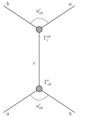
Figure 4: Simple pole diagram associated to Eq. (4.7).

The scattering of the particles $A_{1}$ and $A_{2}$ in the integrable theory is completely determined by the relations

$$A_{i}(\theta_{1})A_{j}(\theta_{2})=\sum_{k,l=1,2}S_{A_{i}A_{j}}^{A_{k}A_{l}}(\theta_{1}-\theta_{2})A_{l}(\theta_{2})A_{k}(\theta_{1})\,\,$$ (4.1)

with the non-zero scattering amplitudes given by [21]

$$S_{A_{1}A_{1}}^{A_{1}A_{1}}(\theta)=S_{A_{2}A_{2}}^{A_{2}A_{2}}(\theta)=\frac{S(\theta)+S_{+}(\theta)}{2}$$

$$S_{A_{1}A_{1}}^{A_{2}A_{2}}(\theta)=S_{A_{2}A_{2}}^{A_{1}A_{1}}(\theta)=\frac{S_{+}(\theta)-S(\theta)}{2}$$

$$S_{A_{1}A_{2}}^{A_{1}A_{2}}(\theta)=S_{A_{2}A_{1}}^{A_{2}A_{1}}(\theta)=\frac{S(\theta)+S_{-}(\theta)}{2}$$

$$S_{A_{1}A_{2}}^{A_{2}A_{1}}(\theta)=S_{A_{2}A_{1}}^{A_{1}A_{2}}(\theta)=\frac{S(\theta)-S_{-}(\theta)}{2}\,\,,$$ (4.2)

where

$$S_{+}(\theta)=-\frac{\sinh\frac{\pi}{2\xi}(\theta+i\pi)}{\sinh\frac{\pi}{2\xi}(\theta-i\pi)}S(\theta)$$

$$S_{-}(\theta)=-\frac{\cosh\frac{\pi}{2\xi}(\theta+i\pi)}{\cosh\frac{\pi}{2\xi}(\theta-i\pi)}S(\theta)$$

$$S(\theta)=-\exp\left\{-i\int_{0}^{\infty}\frac{dx}{x}\frac{\sinh\frac{x}{2}\left(1-\frac{\xi}{\pi}\right)}{\sinh\frac{x\xi}{2\pi}\cosh\frac{x}{2}}\sin\frac{\theta x}{\pi}\right\}$$

$$\xi=\frac{\pi\beta^{2}}{8\pi-\beta^{2}}\,\,.$$

For $\beta^{2}<4\pi$ (attractive regime) the above amplitudes possess simple poles in the physical strip $\mbox{Im}\theta\in(0,\pi)$ corresponding to bound states (breathers) $B_{n}$. The poles are located at $\theta=i(\pi-n\xi)$ ($n$ even for $S_{+}(\theta)$ and odd for $S_{-}(\theta)$) and determine the masses of the breathers

$$m_{n}=2M\sin\frac{n\xi}{2}\,,\hskip 28.45274pt1\leq n<\left[\frac{\pi}{\xi}\right]$$ (4.3)

where $M$ is the mass of the particles $A_{j}$ and $[x]$ denotes the integer part of $x$. The lightest breather $B_{1}$ is the particle interpolated by the boson $\varphi$ and then is odd under all the internal symmetries of the model. The breather $B_{n}$ can be seen as a bound state of $n$ breathers $B_{1}$, so that its symmetry properties are those summarised in Table 2.

Particle	Creating	$Z_{2}\times Z_{2}$	$1\leftrightarrow 2$
	operator
$A_{1}$	$\sigma_{1}\mu_{2}$	$-\times+$	$A_{2}$
$A_{2}$	$\mu_{1}\sigma_{2}$	$+\times-$	$A_{1}$
$B_{2k+1}$	$\sin\beta\varphi$	$-\times-$	$-$
$B_{2k}$	$\cos\beta\varphi$	$+\times+$	$+$

Table 2: Particles, intepolating operators and their symmetries.

The scattering of the breathers with the elementary excitations and with themselves is completely diagonal (initial and final states are identical). The corresponding amplitudes are

$$S_{A_{j}B_{n}}(\theta)=t_{\frac{1}{2}+\frac{n\xi}{2\pi}}(\theta)\times\left\{\begin{array}[]{l}\prod_{j=1}^{(n-1)/2}t^{2}_{\frac{1}{2}+(n-2j)\frac{\xi}{2\pi}}(\theta)\,,\hskip 14.22636ptn\,\,\,\mbox{odd}\\ \\ t_{\frac{1}{2}}(\theta)\prod_{j=1}^{(n-2)/2}t^{2}_{\frac{1}{2}+(n-2j)\frac{\xi}{2\pi}}(\theta)\,,\hskip 14.22636ptn\,\,\,\mbox{even}\\ \end{array}\right.$$ (4.4)

$$S_{B_{m}B_{n}}(\theta)=t_{(m+n)\frac{\xi}{2\pi}}(\theta)t_{1-|m-n|\frac{\xi}{2\pi}}(\theta)\prod_{j=1}^{\mbox{min}\,(m,n)-1}t^{2}_{(|m-n|+2j)\frac{\xi}{2\pi}}(\theta)$$ (4.5)

where

$$t_{\alpha}(\theta)=\frac{\tanh\frac{1}{2}(\theta+i\pi\alpha)}{\tanh\frac{1}{2}(\theta-i\pi\alpha)}\,\,.$$ (4.6)

The simple pole at $\theta=i(\pi+n\xi)/2$ in the amplitude $S_{A_{j}B_{n}}(\theta)$ corresponds to the appearance as a bound state in the channel $A_{j}B_{n}$ of the particle $A_{j+1\,(\mbox{mod}\,2)}$ ($n$ odd) or $A_{j}$ ($n$ even). The simple pole at $\theta=i(n+m)\xi/2$ ($\theta=i[\pi-|n-m|\xi/2]$) in the amplitude $S_{B_{m}B_{n}}(\theta)$ signals that $B_{n+m}$ ($B_{|n-m|}$) appears as a bound state in the $B_{m}B_{n}$ channel.

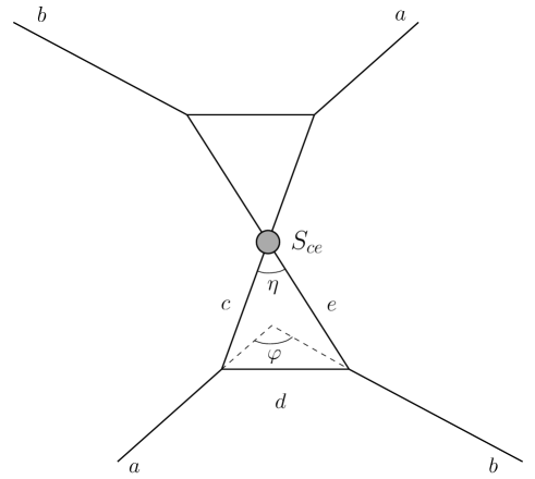
Figure 5: Double pole diagram associated to Eq. (4.8).

A crossed channel pole located at $i\pi-\theta$ is associated to each of these direct channel poles. A direct channel pole at $\theta=iu_{ab}^{c}$ corresponding to the particle $c$ appearing as bound state in the $ab$ channel allows the determination of the three-particle coupling $\Gamma_{ab}^{c}$ through the relation (see Fig. 4)

$$S_{ab}(\theta\simeq iu_{ab}^{c})\simeq i\frac{\Gamma_{ab}^{c}\Gamma_{c}^{ab}}{\theta-iu_{ab}^{c}}\,\,$$ (4.7)

where $\Gamma_{c}^{ab}=C_{a}C_{b}C_{c}\Gamma_{ab}^{c}$, $\Gamma_{ab}^{c}=C_{a}C_{c}\Gamma_{bc}^{a}$ with $C_{A_{j}}=1$, $C_{B_{n}}=(-1)^{n}$. We also note the property $\Gamma_{A_{i}A_{j}}^{B_{n}}=(-1)^{i+j}\Gamma_{A_{j}A_{i}}^{B_{n}}$.

The second order poles do not correspond to bound states and can be explained in terms of multiscattering processes of the type shown in Fig. 5 [22, 23]. In the vicinity of such a pole located at $\theta=i\varphi$ the scattering amplitude can be written as

$$S_{ab}(\theta\simeq i\varphi)\simeq\frac{\Gamma_{ad}^{c}\Gamma_{db}^{e}\Gamma^{ad}_{c}\Gamma^{db}_{e}S_{ce}(i\eta)}{(\theta-i\varphi)^{2}}\,\,.$$ (4.8)

5 Form factors

The knowledge of the scattering amplitudes allows the determination of the form factors

$$F^{\Phi}_{a_{1}\ldots a_{n}}(\theta_{1},\ldots,\theta_{n})=\langle 0|\Phi(0)|a_{1}(\theta_{1})\ldots a_{n}(\theta_{n})\rangle\,\,.$$ (5.1)

Many results are known about the form factors of the sine-Gordon model [9, 10, 11, 12]. Here we will recall how the one- and two-particle form factors can be computed within the general approach. These matrix elements for the order and disorder operators $\sigma_{j}$ and $\mu_{j}$, which are crucial for the description of the Ashkin–Teller model, were first considered in [24].

We use for the two-particle form factors of a scalar operator $\Phi(x)$ the notation

$$F^{\Phi}_{ab}(\theta_{1}-\theta_{2})=\langle 0|\Phi(0)|a(\theta_{1})b(\theta_{2})\rangle\,,$$ (5.2)

the dependence on the rapidity difference being a consequence of Lorentz invariance. The matrix elements satisfy the equations [9, 10, 25]

$$F^{\Phi}_{ab}(\theta)=S_{ab}^{cd}(\theta)F^{\Phi}_{dc}(-\theta)$$ (5.3)

$$F^{\Phi}_{ab}(\theta+2i\pi)=l_{\Phi,a}F^{\Phi}_{ba}(-\theta)$$ (5.4)

$$\mbox{Res}_{\theta=i\pi}F^{\Phi}_{\bar{a}b}(\theta)=i\delta_{ab}\,(1-l_{\Phi,a})\langle\Phi\rangle$$ (5.5)

$$\mbox{Res}_{\theta=iu_{ab}^{c}}F^{\Phi}_{ab}(\theta)=i\Gamma_{ab}^{c}\,F_{c}^{\Phi}$$ (5.6)

where the factor $l_{\Phi,a}$ takes into account the mutual locality between $\Phi$ and the particle $a$ (see Table 3). If $\phi_{a}$ is the operator which interpolates the particle $a$, then $l_{\Phi,a}=e^{2i\pi\gamma_{\Phi,\phi_{a}}}$. For the operators having a bosonic expression, $\gamma_{\Phi,\phi_{a}}$ is given by (3.4). For $\sigma_{j}$ and $\mu_{j}$ the results of Table 3 follow from the properties $l_{\sigma_{j},\sigma_{k}}=l_{\mu_{j},\mu_{k}}=1$ and $l_{\sigma_{j},\mu_{k}}=(-1)^{\delta_{jk}}$ (notice that the even breathers appear in the $A_{j}A_{j}$ channel while the odd ones appear in the $A_{1}A_{2}$ channel).

$\Phi$	Bosonic	$l_{\Phi,A_{j}}$	$l_{\Phi,B_{n}}$
	form
$\sigma_{i}$		$(-1)^{\delta_{ij}+1}$	$(-1)^{n}$
$\mu_{i}$		$(-1)^{\delta_{ij}}$	$(-1)^{n}$
${\cal E}=\varepsilon_{1}+\varepsilon_{2}$	$\cos\beta\varphi$	$+1$	$+1$
${\cal C}=\varepsilon_{1}-\varepsilon_{2}$	$\cos\frac{4\pi}{\beta}\tilde{\varphi}$	$+1$	$+1$
${\cal E}_{+}=\bar{\psi}_{1}\psi_{2}+\bar{\psi}_{2}\psi_{1}$	$\sin\frac{4\pi}{\beta}\tilde{\varphi}$	$+1$	$+1$
${\cal E}_{-}=\bar{\psi}_{1}\psi_{2}-\bar{\psi}_{2}\psi_{1}$	$\sin\beta\varphi$	$+1$	$+1$
${\cal P}=\sigma_{1}\sigma_{2}$	$\sin\frac{\beta}{2}\varphi$	$-1$	$+1$
${\cal P}^{*}=\mu_{1}\mu_{2}$	$\cos\frac{\beta}{2}\varphi$	$-1$	$+1$
$\sigma_{1}\mu_{2}$	$\cos\frac{2\pi}{\beta}\tilde{\varphi}$	$+1$	$+1$
$\mu_{1}\sigma_{2}$	$\sin\frac{2\pi}{\beta}\tilde{\varphi}$	$+1$	$+1$

Table 3: Factors of mutual locality between particles and operators entering Eqs. (5.4) and (5.5).

The form factors are further constrained by the asymptotic bound [26]

$$\lim_{|\theta|\rightarrow\infty}F^{\Phi}_{ab}(\theta)\sim e^{y_{\Phi}|\theta|}$$ (5.7)

$$y_{\Phi}\leq\frac{X_{\Phi}}{2}\,,$$ (5.8)

where $X_{\Phi}$ is the operator scaling dimension. The non-zero two-particle matrix elements on the elementary excitations $A_{1}$ and $A_{2}$ in the disordered phase are then uniquely determined to be

$$F^{\mu_{l}}_{A_{j}A_{j}}(\theta)=\frac{i\pi\langle\mu\rangle}{2\xi\omega(i\pi)}\,\frac{F_{0}(\theta)}{\sinh\frac{\pi}{2\xi}(\theta-i\pi)}\left[\omega(\theta)+(-1)^{l+j}\omega(2i\pi-\theta)\right]$$ (5.9)

$$F^{\cal E}_{A_{j}A_{j}}(\theta)=ic_{1}\,\frac{\cosh\frac{\theta}{2}}{\sinh\frac{\pi}{2\xi}(\theta-i\pi)}\,F_{0}(\theta)$$ (5.10)

$$F^{\cal C}_{A_{j}A_{j}}(\theta)=c_{2}\,(-1)^{j}\,F_{0}(\theta)\,\,$$ (5.11)

$$F^{{\cal E}_{+}}_{A_{1}A_{2}}(\theta)=F^{{\cal E}_{+}}_{A_{2}A_{1}}(\theta)=ic_{2}\,F_{0}(\theta)\,\,$$ (5.12)

$$F^{{\cal E}_{-}}_{A_{1}A_{2}}(\theta)=-F^{{\cal E}_{-}}_{A_{2}A_{1}}(\theta)=-c_{1}\,\frac{\cosh\frac{\theta}{2}}{\cosh\frac{\pi}{2\xi}(\theta-i\pi)}\,F_{0}(\theta)\,\,$$ (5.13)

$$F^{{\cal P}}_{A_{1}A_{2}}(\theta)=-F^{{\cal P}}_{A_{2}A_{1}}(\theta)=-\frac{\pi}{\xi}\langle{\cal P}^{*}\rangle\,\frac{F_{0}(\theta)}{\cosh\frac{\pi}{2\xi}(\theta-i\pi)}\,\,$$ (5.14)

$$F^{{\cal P}^{*}}_{A_{j}A_{j}}(\theta)=\frac{i\pi}{\xi}\langle{\cal P}^{*}\rangle\,\frac{F_{0}(\theta)}{\sinh\frac{\pi}{2\xi}(\theta-i\pi)}\,\,.$$ (5.15)

Here $c_{1}$ and $c_{2}$ are normalisation constants, $\langle\mu\rangle\equiv\langle\mu_{1}\rangle=\langle\mu_{2}\rangle$, and the functions

$$\omega(\theta)=\exp\left\{2\int_{0}^{\infty}\frac{dx}{x}\,\frac{\sinh\left(1-\frac{\xi}{\pi}\right)x}{\sinh\frac{x\xi}{\pi}}\,\frac{\sin^{2}\frac{\theta x}{2\pi}}{\sinh 2x}\right\}$$ (5.16)

$$F_{0}(\theta)=-i\sinh\frac{\theta}{2}\,\exp\left\{\int_{0}^{\infty}\frac{dx}{x}\,\frac{\sinh\frac{x}{2}\left(1-\frac{\xi}{\pi}\right)}{\sinh\frac{x\xi}{2\pi}\,\cosh\frac{x}{2}}\,\frac{\sin^{2}\frac{(i\pi-\theta)x}{2\pi}}{\sinh x}\right\}\,\,$$ (5.17)

satisfy the equations

$$\omega(\theta)=\omega(-\theta)\,\,,\hskip 28.45274pt\omega(\theta+2i\pi)=-\frac{\sinh\frac{\pi}{2\xi}(\theta+i\pi)}{\sinh\frac{\pi}{2\xi}(\theta-i\pi)}\omega(\theta-2i\pi)$$ (5.18)

$$F_{0}(\theta)=S(\theta)F_{0}(-\theta)\,\,,\hskip 28.45274ptF_{0}(\theta+2i\pi)=F_{0}(-\theta)\,\,.$$ (5.19)

For large values of $|\theta|$ they behave as

$$\omega(\theta)\sim\exp\left[\left(\frac{\pi}{\xi}-1\right)\frac{|\theta|}{4}\right]$$ (5.20)

$$F_{0}(\theta)\sim\exp\left[\left(\frac{\pi}{\xi}+1\right)\frac{|\theta|}{4}\right]\,\,.$$ (5.21)

For $\xi<\pi/2$, the analytic continuation

$$\omega(2i\pi-\theta) = -\frac{\sinh[(\theta-i(\pi-2\xi))/4]\sinh[(\theta+i(\pi-2\xi))/4]}{\cos^{2}[(\pi-2\xi)/4]}$$ (5.22)

$$\times \exp\left\{2\int_{0}^{\infty}\frac{dx}{x}\,\frac{\sinh\left(1-\frac{3\xi}{\pi}\right)x}{\sinh\frac{x\xi}{\pi}\sinh 2x}\,\sin^{2}\frac{(2i\pi-\theta)x}{2\pi}\right\}$$

is convergent for real rapidity values.

The breather-breather form factors can be written in the form

$$F^{\Phi}_{B_{n}B_{m}}(\theta)=P^{\Phi}_{B_{n}B_{m}}(\theta)\left(\cosh\frac{\theta}{2}\right)^{\frac{1}{2}(1-l_{\Phi,B_{n}})(-1)^{\delta{n,m}}}\frac{F^{min}_{B_{n}B_{m}}(\theta)}{D_{B_{n}B_{m}}(\theta)}\,\,.$$ (5.23)

Here

$$F^{min}_{B_{m}B_{n}}(\theta)=T_{(m+n)\frac{\xi}{2\pi}}(\theta)T_{1-|m-n|\frac{\xi}{2\pi}}(\theta)\prod_{j=1}^{\mbox{min}\,(m,n)-1}T^{2}_{(|m-n|+2j)\frac{\xi}{2\pi}}(\theta)\,\,.$$ (5.24)

The function

$$T_{\alpha}(\theta)=\exp\left\{2\int_{0}^{\infty}\frac{dt}{t}\frac{\cosh\left(\alpha-\frac{1}{2}\right)t}{\cosh\frac{t}{2}\sinh t}\sin^{2}\frac{(i\pi-\theta)t}{2\pi}\right\}$$ (5.25)

solves the equations

$$T_{\alpha}(\theta)=-t_{\alpha}(\theta)T_{\alpha}(-\theta)\,,\hskip 28.45274ptT_{\alpha}(\theta+2i\pi)=T_{\alpha}(-\theta)$$ (5.26)

and behaves asymptotically as

$$T_{\alpha}(\theta)\sim\exp(|\theta|/2)\,,\hskip 28.45274pt|\theta|\rightarrow\infty\,\,.$$ (5.27)

In particular

$$T_{0}(\theta)=T_{1}(\theta)=-i\sinh\frac{\theta}{2}\,\,.$$ (5.28)

The denominator $D_{B_{n}B_{m}}(\theta)$ in (5.23) accounts for the pole structure of the form factors and can be written as (see [26])

$$D_{B_{m}B_{n}}(\theta)={\cal P}_{(m+n)\frac{\xi}{2\pi}}(\theta){\cal P}_{1-|m-n|\frac{\xi}{2\pi}}(\theta)\prod_{j=1}^{\mbox{min}\,(m,n)-1}{\cal W}_{(|m-n|+2j)\frac{\xi}{2\pi}}(\theta)$$ (5.29)

with

$${\cal P}_{\alpha}(\theta)=\frac{\cos\pi\alpha-\cosh\theta}{2\cos^{2}\frac{\pi\alpha}{2}}\,,\hskip 14.22636pt\alpha\neq 1$$ (5.30)

$${\cal P}_{1}(\theta)=1$$ (5.31)

$${\cal W}_{\alpha}(\theta)={\cal P}_{\alpha}(\theta){\cal P}_{1-\alpha}(\theta)\,\,.$$ (5.32)

The last ingredient of (5.23) are the polynomials

$$P^{\Phi}_{ab}(\theta)=\sum_{k=0}^{N^{\Phi}_{ab}}c^{\Phi;k}_{ab}\,(\cosh\theta)^{k}$$ (5.33)

whose total degree is constrained by the the asymptotic bound (5.8) and whose coefficients are determined by the residue equations (5.5) and (5.6) together with the relation [26]

$$F^{\Phi}_{ab}(\theta\simeq i\varphi)\simeq i\frac{\Gamma_{ad}^{c}\Gamma_{db}^{e}F^{\Phi}_{ce}(i\eta)}{\theta-i\varphi}$$ (5.34)

associated to the double poles (4.8) in the scattering amplitudes. In particular, one finds $N_{B_{1}B_{1}}^{\Phi}=0$ and $N_{B_{2}B_{2}}^{\Phi}=1$ for $\Phi=\mu,\,{\cal E},\,{\cal P}^{*}$, and $N_{B_{1}B_{2}}^{\cal P}=1$.

Concerning the channel $A_{j}B_{n}$, the property

$$F^{\Phi}_{A_{j}B_{n}}(\theta)=(-1)^{n}F^{\Phi}_{B_{n}A_{j}}(\theta)$$ (5.35)

has to be taken into account. We find that the minus sign appearing for odd breathers (and implying $\Gamma_{A_{j}B_{2k+1}}^{A_{j+1\,(mod\,2)}}=-\Gamma_{B_{2k+1}A_{j}}^{A_{j+1\,(mod\,\,2)}}$) is needed if solutions compatible with the asymptotic bound (5.8) are to be found for the operators $\sigma_{i}$ and $\sigma_{i}\mu_{i+1\,(mod\,2)}$. Then one can write

$$F^{\Phi}_{A_{j}B_{n}}(\theta)=P^{\Phi}_{A_{j}B_{n}}(\theta)\left(\cosh\frac{\theta}{2}\right)^{\delta_{n,odd}\delta_{1,l_{\Phi,B_{n}}}}\frac{F^{min}_{A_{j}B_{n}}(\theta)}{D_{A_{j}B_{n}}(\theta)}\,,$$ (5.36)

where

$$F^{min}_{A_{j}B_{n}}(\theta)=\prod_{j=0}^{n-1}T_{\frac{1}{2}+(n-2j)\frac{\xi}{2\pi}}(\theta)$$ (5.37)

$$D_{A_{j}B_{n}}(\theta)={\cal P}_{\frac{1}{2}+\frac{n\xi}{2\pi}}(\theta)\times\left\{\begin{array}[]{l}\prod_{j=1}^{(n-1)/2}{\cal W}_{\frac{1}{2}+(n-2j)\frac{\xi}{2\pi}}(\theta)\,,\hskip 14.22636ptn\,\,\,\mbox{odd}\\ \\ {\cal P}_{\frac{1}{2}}(\theta)\prod_{j=1}^{(n-2)/2}{\cal W}_{\frac{1}{2}+(n-2j)\frac{\xi}{2\pi}}(\theta)\,,\hskip 14.22636ptn\,\,\,\mbox{even}\\ \end{array}\right.$$ (5.38)

and $P^{\Phi}_{A_{j}B_{n}}(\theta)$ are polynomials in $\cosh\theta$ to be fixed through the conditions on the poles. In particular we have

$$F_{A_{j}B_{1}}^{\sigma_{j+1\,(mod\,2)}}(\theta)=-F_{B_{1}A_{j}}^{\sigma_{j+1\,(mod\,2)}}(\theta)=(-1)^{j}\,a\,\frac{T_{(1+\xi/\pi)/2}(\theta)}{{\cal P}_{(1+\xi/\pi)/2}(\theta)}$$ (5.39)

$$F_{A_{j}B_{2}}^{\sigma_{j}}(\theta)=F_{B_{2}A_{j}}^{\sigma_{j}}(\theta)=(b\cosh\theta+c)\,\frac{T_{1/2}(\theta)T_{1/2+\xi/\pi}(\theta)}{{\cal P}_{1/2}(\theta){\cal P}_{1/2+\xi/\pi}(\theta)}$$ (5.40)

with $a$, $b$ and $c$ determined by the equations

$$\mbox{Res}_{\theta=i(\pi+\xi)/2}F^{\sigma_{2}}_{A_{1}B_{1}}(\theta)=i\Gamma^{A_{2}}_{A_{1}B_{1}}F^{\sigma_{2}}_{A_{2}}$$ (5.41)

$$\mbox{Res}_{\theta=i(\pi/2+\xi)}F^{\sigma_{2}}_{A_{2}B_{2}}(\theta)=i\Gamma^{A_{2}}_{A_{2}B_{2}}F^{\sigma_{2}}_{A_{2}}$$ (5.42)

$$\mbox{Res}_{\theta=i\pi/2}F^{\sigma_{2}}_{A_{2}B_{2}}(\theta)=i\Gamma^{A_{1}}_{A_{2}B_{1}}\Gamma^{B_{1}}_{B_{1}B_{2}}F^{\sigma_{2}}_{A_{1}B_{1}}(i(\pi-3\xi)/2)\,\,.$$ (5.43)

The last equation is the specialisation of (5.34) to the double pole appearing at $\theta=i\pi/2$ in the $A_{j}B_{2k}$ scattering amplitudes and related to the diagram of Fig. 5 with $a=A_{j}$, $b=B_{2k}$, $d=e=B_{k}$ and $c=A_{i}$, $i=j$ ($i\neq j$) for $k$ even (odd). It can be checked that the matrix elements (5.40) determined in this way satisfy the asymptotic factorisation condition [28]

$$\lim_{\theta\rightarrow\infty}F^{\sigma_{j}}_{A_{j}B_{2k}}(\theta)=F^{\sigma_{j}}_{A_{j}}\frac{F^{\mu_{i}}_{B_{2k}}}{\langle\mu\rangle}$$ (5.44)

with $k=1$. The condition

$$\lim_{\theta\rightarrow\infty}\left|F^{\mu_{1}\pm\mu_{2}}_{A_{j}A_{j}}(\theta)\right|=\frac{(F^{\sigma_{j}}_{A_{j}})^{2}}{\langle\mu\rangle}$$ (5.45)

fixes the relative normalisation between order and disorder operators.

6 Correlation functions

Within the form factor approach, correlation functions are obtained through the spectral sum

$$\langle\Phi_{1}(x)\Phi_{2}(0)\rangle = \sum_{n=0}^{\infty}\sum_{a_{1},\ldots,a_{n}}\int_{\theta_{1}>\ldots>\theta_{n}}\frac{d\theta_{1}}{2\pi}\ldots\frac{d\theta_{n}}{2\pi}$$ (6.1)

$$\langle 0|\Phi_{1}(0)|a_{1}(\theta_{1})\ldots a_{n}(\theta_{n})\rangle\langle a_{n}(\theta_{n})\ldots a_{1}(\theta_{1})|\Phi_{2}(0)|0\rangle e^{-E_{n}|x|}\,,$$

where

$$E_{n}=\sum_{k=1}^{n}m_{a_{k}}\cosh\theta_{k}$$ (6.2)

denotes the total energy of the $n$-particle asymptotic state.

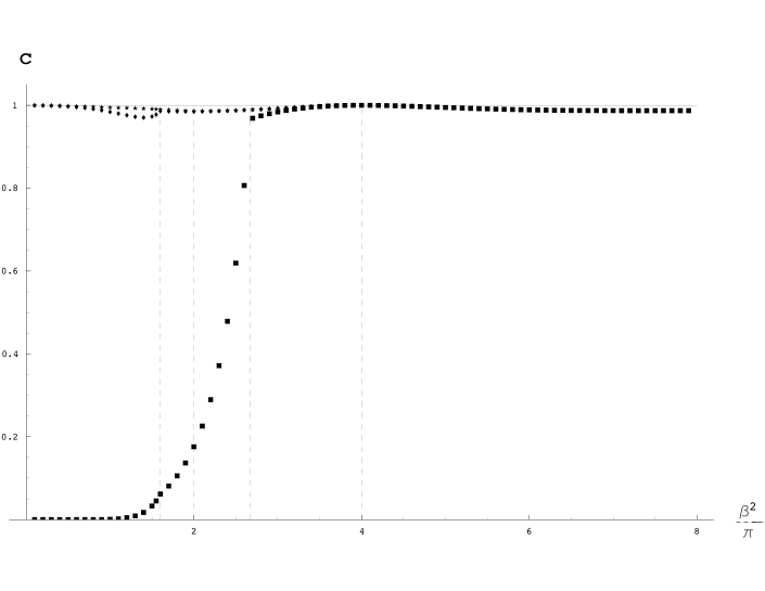
Figure 6: Different approximations of the central charge coming from Eqs. (6.3) and (6.1). The squares indicate the contribution of the states $A_{j}A_{j}$ only, the diamonds the inclusion of the states $B_{2}$ and $B_{1}B_{1}$, the stars the inclusion of the states $B_{4}$, $B_{1}B_{3}$ and $B_{2}B_{2}$. The exact result is $c=1$. From right to left, the dashed vertical lines correspond to the first four thresholds where the breather $B_{n}$ ($n=1,\ldots,4$) enters the spectrum of asymptotic particles.

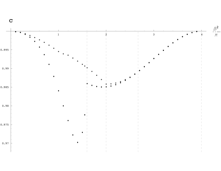
Figure 7: A detail of Fig. 6.

This large distance expansion can produce good approximations of the integrated correlators even when only few lightest states are included in the sum. A quantitative illustration of the convergence pattern is obtained using the spectral sum to compute exactly known quantities like the central charge $c$ and the scaling dimensions $X_{\Phi}$ through the sum rules [27, 28]

$$c = \frac{3}{4\pi}\int d^{2}x\,|x|^{2}\langle\Theta(x)\Theta(0)\rangle_{c}$$ (6.3)

$$X_{\Phi} = -\frac{1}{2\pi\langle\Phi\rangle}\int d^{2}x\,\langle\Theta(x)\Phi(0)\rangle_{c}\,\,,$$ (6.4)

where $\langle\cdots\rangle_{c}$ denotes connected correlators and $\Theta(x)$ is the trace of the stress-energy tensor. The latter is proportional to the energy operator ${\cal E}(x)$ and its form factors are normalised through the condition

$$F^{\Theta}_{aa}(i\pi)=2\pi m_{a}^{2}\,\,.$$ (6.5)

Moreover, for $a\neq b$, $P^{\Theta}_{ab}(\theta)$ factorises a term [26]

$$\cosh\theta+\frac{m_{a}^{2}+m_{b}^{2}}{2m_{a}m_{b}}\,\,.$$ (6.6)

The asymptotic condition [28]

$$\lim_{\theta\rightarrow\infty}F^{\Theta}_{B_{n}B_{n}}(\theta)=\frac{(F^{\Theta}_{B_{n}})^{2}}{\langle\Theta\rangle}$$ (6.7)

can be used to determine the expectation value

$$\langle\Theta\rangle=-\pi M^{2}\tan\frac{\xi}{2}\,,$$ (6.8)

a result which coincides with that known from the thermodynamic Bethe ansatz (see [29]).

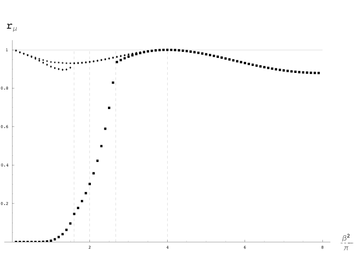
Figure 8: The ratio (6.9) for the operators $\mu_{j}$ coming from Eqs. (6.4) and (6.1). The squares indicate the contribution of the states $A_{j}A_{j}$ only, the diamonds the inclusion of the states $B_{2}$ and $B_{1}B_{1}$, the stars the inclusion of the state $B_{4}$.

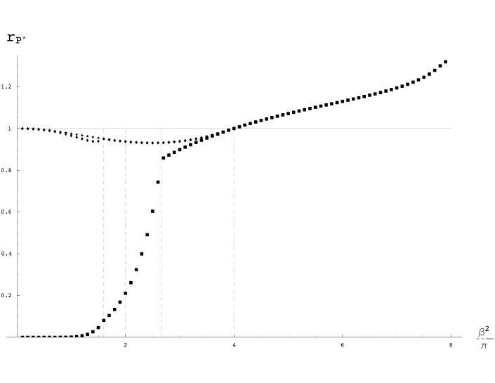
Figure 9: As in Fig. 8 for the operator ${\cal P}^{*}$.

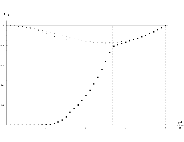
Figure 10: As in Fig. 8 for the operator ${\cal E}$.

Figures 6 and 7 show the first few approximations provided by the insertion of a truncated spectral sum into the formula (6.3) for the central charge. For this quantity as for the scaling dimensions computed through (6.4), the states $A_{j}A_{j}$ yield the exact result at the free fermion point $\beta^{2}=4\pi$, as well as the state $B_{1}B_{1}$ gives the exact result at the free boson point $\beta^{2}=0$. Away from these free points the convergence of the series is extremely rapid due to the factor $|x|^{2}$ in (6.3) which suppresses the contribution to the integral of the short distances, namely the region where the truncated spectral series fails to reproduce the exact correlator. Hence, in the repulsive region $4\pi<\beta^{2}<8\pi$ the $A_{j}A_{j}$ contribution reproduces the exact result with a maximal deviation which is slightly above $1\%$ as $\beta^{2}\rightarrow 8\pi$. Entering the attractive region below the free fermion point this contribution falls down quite rapidly as the particles $A_{j}$ become heavier than the lowest breathers (see (4.3)). The inclusion of the first few breather states, however, gives a quite accurate result also in the repulsive region (Fig. 7).

The same qualitative pattern can be observed in Figs. 8, 9 and 10 showing results for the ratios

$$r_{\Phi}=\frac{X_{\Phi}^{approx}}{X_{\Phi}}$$ (6.9)

between the approximations for the scaling dimensions obtained inserting a truncated spectral series in (6.4) and the exact values. Quantitatively, the absence of the ultraviolet suppressing factor in (6.4) as compared to (6.3) obviously leads to poorer results for a given level of truncation. Of course, the accuracy can be improved by including more states in the spectral sum. Here we simply observe that the increasing deviation from the exact value for larger values of $\beta^{2}$ in the repulsive region is due to the increasing ultraviolet singularities of the exact correlators entering the sum rules, what makes increasingly important the contribution of the short distances to the integrals. The result for $r_{\cal E}=r_{\Theta}$ is plotted up to the free fermion point because the corresponding integral in (6.4) diverges for $\beta^{2}\geq 4\pi$ (see [28]). The integral entering the computation of $r_{{\cal P}^{*}}$ becomes divergent at $\beta^{2}=8\pi$, what helps understanding why the two-particle approximation is particularly poor as this point is approached.

7 Universal ratios

The ability to compute the correlation functions allows the evaluation of the canonical thermodynamic observables. We will consider the magnetisations

$$M_{\sigma}=|\langle\sigma_{j}\rangle|$$ (7.1)

$$M_{\cal P}=|\langle{\cal P}\rangle|$$ (7.2)

the specific heat

$$C=\int d^{2}x\,\langle{\cal E}(x){\cal E}(0)\rangle_{c}$$ (7.3)

the susceptibilities

$$\chi_{\sigma}=\int d^{2}x\,\langle\sigma_{j}(x)\sigma_{j}(0)\rangle_{c}$$ (7.4)

$$\chi_{12}=\left|\int d^{2}x\,\langle\sigma_{1}(x)\sigma_{2}(0)\rangle_{c}\right|$$ (7.5)

$$\chi_{\cal P}=\int d^{2}x\,\langle{\cal P}(x){\cal P}(0)\rangle_{c}$$ (7.6)

the second moment correlation lengths

$$\xi^{2nd}_{\sigma}=\left(\frac{1}{4\chi_{\sigma}}\int d^{2}x\,|x|^{2}\langle\sigma_{j}(x)\sigma_{j}(0)\rangle_{c}\right)^{1/2}$$ (7.7)

$$\xi^{2nd}_{\cal P}=\left(\frac{1}{4\chi_{\cal P}}\int d^{2}x\,|x|^{2}\langle{\cal P}(x){\cal P}(0)\rangle_{c}\right)^{1/2}$$ (7.8)

and the exponential correlation lengths $\xi_{\Phi}$ defined as

$$\lim_{|x|\rightarrow\infty}\langle\sigma_{j}(x)\sigma_{j}(0)\rangle_{c}\sim e^{-|x|/\xi_{\sigma}}$$ (7.9)

$$\lim_{|x|\rightarrow\infty}\langle{\cal P}(x){\cal P}(0)\rangle_{c}\sim e^{-|x|/\xi_{\cal P}}\,\,.$$ (7.10)

These quantities can be evaluated on the two sides of the critical line with continously varying exponents. In the disordered phase II we decompose the above correlators onto the form factors of section 5. Duality is exploited to obtain the results for the ferromagnetic phase I: the operators are replaced by their duals and the correlators are again decomposed over the form factors of section 5; the observables above do not depend on which of the four ferromagnetic ground states is selected by spontaneous symmetry breaking.

For a given observable ${\cal F}$, we denote by ${\cal F}^{+}$ its limit toward a given point on the critical line along a path in phase II, and by ${\cal F}^{-}$ the limit toward the same point along the dual path in phase I. Dimensionless numbers independent on metric factors can be obtained suitably combining the limits toward the same fixed point of different observables. These numbers are universal and characterise the scaling region around the critical line with continously varying exponents.

Some of these universal combinations can be determined exactly. It follows from the spectral decomposition (6.1) that the exponential correlation length $\xi_{\Phi}$ is simply the inverse mass of the lightest asymptotic state coupling to the operator $\Phi$. In the disordered phase the lightest state is $A_{j}$ for $\sigma_{j}$; for ${\cal P}$ we have instead $A_{1}A_{2}$ in the repulsive region $\beta^{2}>4\pi$ (i.e. $\xi>\pi$) and $B_{1}$ in the attractive region. In the ferromagnetic phase, both $\sigma_{j}$ and ${\cal P}$ (or equivalently $\mu_{j}$ and ${\cal P}^{*}$ in the disordered phase) couple to $A_{j}A_{j}$ for $\beta^{2}>8\pi/3$ (i.e. $\xi>\pi/2$) and to $B_{2}$ below this threshold. The following universal ratios then follow from (4.3)

$$\frac{\xi^{+}_{\sigma}}{\xi^{-}_{\sigma}}=\left\{\begin{array}[]{l}2\,,\hskip 14.22636pt\xi>\pi/2\\ \\ 2\sin\xi\,,\hskip 14.22636pt\xi<\pi/2\\ \end{array}\right.$$ (7.11)

$$\frac{\xi^{+}_{\cal P}}{\xi^{-}_{\cal P}}=\left\{\begin{array}[]{l}1\,,\hskip 14.22636pt\xi>\pi\\ \\ 1/\sin\frac{\xi}{2}\,,\hskip 14.22636pt\frac{\pi}{2}<\xi<\pi\\ \\ 2\cos\frac{\xi}{2}\,,\hskip 14.22636pt\xi<\frac{\pi}{2}\\ \end{array}\right.$$ (7.12)

$$\frac{\xi^{+}_{\sigma}}{\xi^{+}_{\cal P}}=\left\{\begin{array}[]{l}2\,,\hskip 14.22636pt\xi>\pi\\ \\ 2\sin\frac{\xi}{2}\,,\hskip 14.22636pt\xi<\pi\,\,.\\ \end{array}\right.$$ (7.13)

The fact that the energy operator ${\cal E}$ is odd under duality and the specific heat is bilinear in ${\cal E}$ implies

$$C^{+}/C^{-}=1\,\,.$$ (7.14)

The combination

$$C^{+}\;(\xi_{\sigma}^{+})^{2}=-(1-\alpha)(2-\alpha)\frac{\langle\Theta\rangle}{4\pi M^{2}}\,,$$ (7.15)

where $\alpha=1-\frac{\xi}{\pi}$ is the specific heat critical exponent and $\langle\Theta\rangle$ is given in (6.8), is also exact.

$\beta^{2}/\pi$	$\frac{\xi^{2nd\,\,+}_{\sigma}}{\xi_{\sigma}^{+}}$	$\frac{\xi^{2nd\,\,+}_{\sigma}}{\xi^{2nd\,\,-}_{\sigma}}$	$\chi_{\sigma}^{+}/\chi_{\sigma}^{-}$	$\chi_{12}^{-}/\chi_{\sigma}^{-}$	$R_{\sigma}$	$\frac{\xi^{2nd\,\,+}_{\cal P}}{\xi_{\sigma}^{+}}$	$\frac{\xi^{2nd\,\,+}_{\cal P}}{\xi^{2nd\,\,-}_{\cal P}}$	$\chi^{+}_{\cal P}/\chi^{-}_{\cal P}$	$R_{\cal P}$
2.0	0.9905	1.964	11.59	0.9411	1.434	0.9905	1.964	11.59	1.434
2.1	0.9923	2.070	13.42	0.9212	1.501	0.9322	1.931	10.79	1.320
2.2	0.9938	2.176	15.33	0.8970	1.563	0.8795	1.897	10.06	1.218
2.3	0.9950	2.279	17.32	0.8685	1.619	0.8316	1.863	9.392	1.125
2.4	0.9961	2.381	19.33	0.8353	1.670	0.7880	1.829	8.774	1.040
2.5	0.9970	2.479	21.36	0.7976	1.717	0.7482	1.795	8.202	0.9626
2.6	0.9978	2.573	23.35	0.7555	1.758	0.7117	1.760	7.670	0.8915
8/3	0.9983	2.634	24.64	0.7250	1.784	0.6891	1.737	7.334	0.8473
2.7	0.9984	2.662	25.29	0.7093	1.796	0.6781	1.725	7.175	0.8264
2.8	0.9988	2.745	27.15	0.6595	1.830	0.6470	1.689	6.720	0.7672
2.9	0.9991	2.821	28.89	0.6065	1.861	0.6181	1.654	6.295	0.7127
3.0	0.9993	2.890	30.51	0.5511	1.888	0.5915	1.618	5.897	0.6623
3.1	0.9995	2.950	31.96	0.4939	1.911	0.5668	1.583	5.525	0.6156
3.2	0.9997	3.002	33.26	0.4356	1.931	0.5438	1.548	5.175	0.5724
3.3	0.9998	3.046	34.38	0.3769	1.948	0.5224	1.513	4.847	0.5323
3.4	0.9999	3.081	35.33	0.3184	1.963	0.5026	1.479	4.538	0.4950
3.5	0.9999	3.110	36.10	0.2608	1.975	0.4840	1.445	4.247	0.4602
3.6	1.000	3.131	36.71	0.2045	1.984	0.4668	1.412	3.972	0.4278
3.7	1.000	3.146	37.16	0.1500	1.991	0.4506	1.380	3.711	0.3976
3.8	1.000	3.155	37.47	0.09763	1.996	0.4355	1.349	3.464	0.3694
3.9	1.000	3.161	37.64	0.04756	1.999	0.4214	1.319	3.228	0.3430
4.0	1	3.162	37.70	0	2	0.4082	1.291	3	0.3183
4.1	1.000	3.161	37.65	0.04494	1.999	0.3959	1.264	2.782	0.2952
4.2	1.000	3.157	37.50	0.08721	1.996	0.3843	1.238	2.579	0.2736
4.3	1.000	3.152	37.28	0.1268	1.992	0.3735	1.213	2.389	0.2533
4.4	1.000	3.145	36.98	0.1637	1.986	0.3634	1.189	2.211	0.2343
4.5	1.000	3.138	36.63	0.1981	1.979	0.3539	1.165	2.044	0.2165
4.6	1.000	3.130	36.23	0.2299	1.971	0.3450	1.142	1.887	0.1998
4.7	1.000	3.122	35.78	0.2594	1.961	0.3366	1.120	1.740	0.1841
4.8	1.000	3.114	35.30	0.2866	1.950	0.3288	1.099	1.603	0.1694
4.9	1.000	3.105	34.80	0.3117	1.937	0.3215	1.078	1.473	0.1556
5.0	1.000	3.097	34.28	0.3348	1.924	0.3147	1.059	1.352	0.1427
5.1	1.000	3.090	33.74	0.3560	1.909	0.3082	1.040	1.238	0.1306
5.2	1.000	3.082	33.18	0.3754	1.893	0.3022	1.022	1.132	0.1193
5.3	1.000	3.075	32.62	0.3932	1.877	0.2966	1.005	1.032	0.1087
5.4	1.000	3.069	32.05	0.4095	1.859	0.2914	0.9894	0.9383	0.09876
5.5	1.000	3.063	31.48	0.4244	1.840	0.2865	0.9742	0.8509	0.08950
5.6	1.000	3.057	30.91	0.4380	1.821	0.2819	0.9599	0.7691	0.08086
5.7	1.000	3.052	30.33	0.4503	1.800	0.2776	0.9463	0.6929	0.07280
5.8	1.000	3.047	29.76	0.4616	1.778	0.2736	0.9336	0.6218	0.06530
5.9	1.000	3.043	29.18	0.4719	1.756	0.2699	0.9216	0.5557	0.05834
6.0	1.000	3.039	28.60	0.4812	1.732	0.2664	0.9104	0.4944	0.05188

Table 4: Two-particle approximation for the universal ratios along the Ashkin-Teller critical line. The relation between $\beta$ and the values of the lattice couplings $J$ and $J_{4}$ at the corresponding critical point is provided by Eqs. (3.13) and (2.3). The values $\beta^{2}/\pi=2,8/3,4$ correspond to the $4$-state Potts, decoupled Ising and Fateev-Zamolodchikov models, respectively.

The universal ratios involving the susceptibilities and second moment correlation lengths cannot be computed exactly. In Table 4 we list the results provided by the form factor approach including in the spectral series all the one and two-particle states (two-particle approximation). The quantities $R_{\sigma}$ and $R_{\cal P}$ are defined as

$$R_{\Phi}=\frac{\chi_{\Phi}^{+}}{(\xi_{\sigma}^{+}M_{\Phi}^{-})^{2}}\,\,.$$ (7.16)

An important indication about the size of the error involved in the two-particle approximation comes from the comparison with the exact results [30] avalaible for the point $\beta^{2}=4\pi$, where the system reduces to two decoupled Ising models. We stress that, although the theory at this point is free, the opearators $\sigma_{j}$ and ${\cal P}$ belong to the non–trivial sector and have non–zero form factors on an arbitrary number of particles. Hence, the results obtained for their correlators are representative of what happens at generic values of $\beta$. Table 5 shows that the error of the two–particle approximation is extremely small (less than $0.1\%$) for the ratios involving $\sigma_{j}$ only, while it grows to order $1\%$ for the ratios involving ${\cal P}$. This fact has a very clear origin. The spectral representation we use for the correlators is a large distance expansion and when we truncate it to obtain approximated results we make an error on the ‘short’ distances. Hence, the error on the integrals over all distance scales grows with the strength of the ultraviolet singularities of the correlators, namely with the scaling dimensions of the operators. The scaling dimension of ${\cal P}$ is twice that of $\sigma_{j}$ at $\beta^{2}=4\pi$ and this explains the two different error scales.

On these grounds we expect that the error on the ratios involving only $\sigma_{j}$ will stay quite small along the whole critical line, as a consequence of the fact that the scaling dimension of this operator does not depend on $\beta$. Concerning the ratios involving ${\cal P}$, the value $X_{\cal P}=\frac{\beta^{2}}{16\pi}$ suggests that the error will be of the same size of that of the $\sigma$–ratios at $\beta^{2}=2\pi$ and then will increase with $\beta$ to values that (from the results of the previous section) should not exceed $10\%$ at $\beta^{2}=6\pi$.

Ratio	Two-particle	Exact
	approximation
$\xi_{\sigma}^{2nd\,+}/\xi_{\sigma}^{+}$	$1$	$0.999598087..$
$\xi_{\sigma}^{2nd\,+}/\xi_{\sigma}^{2nd\,-}$	$3.1623$	$3.16249504..$
$\chi_{\sigma}^{+}/\chi_{\sigma}^{-}$	$37.699$	$37.6936520..$
$R_{\sigma}$	$2$	$2.00163051..$
$\xi_{\cal P}^{2nd\,+}/\xi_{\sigma}^{+}$	$0.408$	$0.40656..$
$\xi_{\cal P}^{2nd\,+}/\xi_{\cal P}^{2nd\,-}$	$1.291$	$1.3088..$
$\chi_{\cal P}^{+}/\chi_{\cal P}^{-}$	$3$	$2.9108..$
$R_{\cal P}$	$0.318$	$0.32104..$

Table 5: Universal ratios at the Ising decoupling point $\beta^{2}=4\pi$.

For $\beta^{2}=2\pi$ the results we obtained should reproduce those for the $4$-state Potts model. In order to check this point we label $\alpha=(\alpha_{1},\alpha_{2})$, with $\alpha_{1,2}=\pm 1$, the four states in which each site of the lattice can be. Then we build out of the Ashkin–Teller spin variables $\sigma_{1}$ and $\sigma_{2}$ the site variable $\sigma=(\sigma_{1},\sigma_{2})$ and introduce the traditional Potts spin variables

$$s_{\alpha}(x) = \delta_{\sigma(x),\alpha}-\frac{1}{4}$$ (7.17)

$$= \frac{1}{4}[\alpha_{1}\sigma_{1}(x)+\alpha_{2}\sigma_{2}(x)+\alpha_{1}\alpha_{2}\sigma_{1}\sigma_{2}(x)]$$

satisfying $\sum_{\alpha}s_{\alpha}=0$. If we denote by $|0_{\gamma}\rangle$ the ground state that spontaneous symmetry breaking has selected in the ferromagnetic phase I, we will have

$$\langle 0_{\gamma}|s_{\alpha}(x)s_{\alpha}(0)|0_{\gamma}\rangle = \frac{1}{16}\langle 0_{\gamma}|\sigma_{1}(x)\sigma_{1}(0)+\sigma_{2}(x)\sigma_{2}(0)+\sigma_{1}\sigma_{2}(x)\sigma_{1}\sigma_{2}(0)+2\alpha_{1}\alpha_{2}\sigma_{1}(x)\sigma_{2}(0)$$ (7.18)

$$+ 2\alpha_{2}\sigma_{1}(x)\sigma_{1}\sigma_{2}(0)+2\alpha_{1}\sigma_{2}(x)\sigma_{1}\sigma_{2}(0)|0_{\gamma}\rangle\,\,.$$

Along the Potts trajectory the internal symmetry is enhanced to invariance under global permutations of the four colours and one finds the expression

$$\langle 0_{(1,1)}|s_{\alpha}(x)s_{\alpha}(0)|0_{(1,1)}\rangle_{Potts}=$$

$$\frac{1}{16}\langle 0_{(1,1)}|3\sigma_{1}(x)\sigma_{1}(0)+2(\alpha_{1}\alpha_{2}+\alpha_{2}+\alpha_{1})\sigma_{1}(x)\sigma_{2}(0)|0_{(1,1)}\rangle_{Potts}=$$

$$\frac{1}{16}\langle 0_{(1,1)}|3\sigma_{1}(x)\sigma_{1}(0)+2(4\delta_{\alpha,{(1,1)}}-1)\sigma_{1}(x)\sigma_{2}(0)|0_{(1,1)}\rangle_{Potts}\,\,$$ (7.19)

explicitely showing that only the cases $\alpha=\gamma$ and $\alpha\neq\gamma$ are distinguished in the correlator $\langle 0_{\gamma}|s_{\alpha}(x)s_{\alpha}(0)|0_{\gamma}\rangle$. In the disordered phase mixed correlators vanish by symmetry and we have

$$\langle s_{\alpha}(x)s_{\alpha}(0)\rangle_{Potts}=\frac{3}{16}\langle\sigma_{1}(x)\sigma_{1}(0)\rangle_{Potts}\,\,.$$ (7.20)

In the Potts model we define the longitudinal spontaneous magnetisation

$$M=\langle 0_{\alpha}|s_{\alpha}|0_{\alpha}\rangle\,,$$ (7.21)

the high-temperature susceptibility

$$\chi=\int d^{2}x\,\langle s_{\alpha}(x)s_{\alpha}(0)\rangle_{c}\,,$$ (7.22)

the low-temperature longitudinal and transverse susceptibilities

$$\chi_{L}=\int d^{2}x\,\langle 0_{\alpha}|s_{\alpha}(x)s_{\alpha}(0)|0_{\alpha}\rangle_{c}$$ (7.23)

$$\chi_{T}=\int d^{2}x\,\langle 0_{\alpha}|s_{\gamma}(x)s_{\gamma}(0)|0_{\alpha}\rangle_{c}\hskip 28.45274pt\alpha\neq\gamma$$ (7.24)

and the second moment and exponential correlation lengths $\xi^{2nd}$ and $\xi$ computed from the correlator $\langle s_{\alpha}(x)s_{\alpha}(0)\rangle$ at high temperature and $\langle 0_{\alpha}|s_{\alpha}(x)s_{\alpha}(0)|0_{\alpha}\rangle$ at low temperature.
The relations between these quantities and the Ashkin-Teller observables follow from Eqs. (7.17), (7.19) and (7.20). In particular one obtains

$$\chi^{+}/\chi_{L}^{-}=\left[\frac{\chi_{\sigma}^{+}/\chi_{\sigma}^{-}}{1+2\chi_{12}^{-}/\chi_{\sigma}^{-}}\right]_{\beta^{2}=2\pi}\simeq 4.02$$ (7.25)

$$\chi^{-}_{T}/\chi_{L}^{-}=\left[\frac{1-\frac{2}{3}\chi_{12}^{-}/\chi_{\sigma}^{-}}{1+2\chi_{12}^{-}/\chi_{\sigma}^{-}}\right]_{\beta^{2}=2\pi}\simeq 0.129\,\,.$$ (7.26)

These results agree with those of Refs. [31, 32] where the amplitude ratios for the $q$-state Potts model were computed. This non-trivial check eliminates the doubt raised in [32] about the result of [31] for the ratio $\chi^{+}/\chi_{L}^{-}$ in the $q$-state Potts model. For $q=3$ full agreement with the theoretical prediction was found in the lattice studies of Refs. [33, 34].

8 Conclusion

We have computed the universal ratios along the Ashkin-Teller critical line with continously varying exponents using the field theoretical description of the scaling limit provided by the sine-Gordon model. As discussed in the Introduction, these results can be tested through numerical simulation or series expansions on the lattice model. Up to now, lattice results for the universal ratios along the Ashkin-Teller critical line exist only for the particular cases of the Ising decoupling point (where the exact values are known, see Table 5) and of the 4-state Potts model [35, 34]. In the latter case the lattice results are compatible with the field theoretical predictions but are affected by large uncertainties originated by logarthmic corrections to scaling [36, 37] coming from the marginal operator that is responsible for the end of critical line at the Potts point. Reducing the error bars at this point as well as obtaining estimates at other points along the Ashkin-Teller critical line appear as challanging tasks for future lattice studies.

Acknowledgements. This work was partially supported by the European Commission TMR programme HPRN-CT-2002-00325 (EUCLID). The work of P.G. is supported by the COFIN “Teoria dei Campi, Meccanica Statistica e Sistemi Elettronici”.

References

[1] V. Privman, P.C. Hohenberg and A. Aharony, Universal critical
point amplitude relations, in Phase transition and critical phenomena,
Vol. 14, ed. C. Domb and J.L. Lebowitz (Academic Press, New York, 1991).
[2] A.A. Belavin, A.M. Polyakov and A.B. Zamolodchikov, Nucl. Phys.
B 241 (1984) 333.
[3] D. Friedan, Z. Qiu and S. Shenker, Phys. Rev. Lett. 52 (1984)
1575.
[4] J. Ashkin and E. Teller, Phys. Rev. 64 (1943) 178.
[5] R.J. Baxter, Exactly solved models in statistical
mechanics (Academic Press, New York, 1982).
[6] F.J. Wegner, J. Phys. C 5 (1972) L131.
[7] L.P. Kadanoff and A.C. Brown, Ann. Phys. 121 (1979) 318.
[8] L.P. Kadanoff, Phys. Rev. B 22 (1980) 1405.
[9] M. Karowski, P. Weisz, Nucl. Phys. B 139 (1978) 445.
[10] F.A. Smirnov, Form Factors in Completely Integrable
Models of Quantum Field Theory (World Scientific) 1992.
[11] S. Lukyanov, Mod. Phys. Lett. A 12 (1997) 2543.
[12] S. Lukyanov and A.B. Zamolodchikov, Nucl. Phys. B 607 (2001) 437.
[13] C. Fan, Phys. Lett. A 39 (1972) 136.
[14] S.J. Ferreira and A.D. Sokal, Phys. Rev. B 51 (1995) 6727.