Non BPS Noncommutative Vortices

Abstract

We construct exact vortex solutions to the equations of motion of the Abelian Higgs model defined in non commutative space, analyzing in detail the properties of these solutions beyond the BPS point. We show that our solutions behave as smooth deformations of vortices in ordinary space time except for parity symmetry breaking effects induced by the non commutative parameter $\theta$.

1 Introduction

The study of noncommutative solitons and instantons -finite energy or finite action solutions to the classical equations of motion of noncommutative field theories- has been a field of intense activity after the revival of interest in these theories in connection with strings and brane dynamics (see [1]-[3] and references therein). In fact, the first explicit instanton solutions that were constructed in four dimensional Yang-Mills theory [4] strongly influenced developments in string quantization [5]. Concerning solitons, not only the noncommutative counterparts of vortex, monopoles and other localized solutions in ordinary space were constructed but regular stable solutions which become singular in the commutative limit were also discovered [6]-[21].

Most of these solitons correspond to selfdual/anti-selfdual (BPS) solutions which are more simple to obtain than those arising from the Euler Lagrange (EL) equations of motion. Moreover, in even dimensional spaces, calculations can be simplified by exploiting the connection between noncommutative Moyal product in configuration space and a Hilbert space representation which realizes noncommutativity in terms of creation and annihilation operators acting on a Fock space.

Among the BPS soliton solutions that have been obtained in this way, particular interest has attracted the construction of noncommutative BPS vortices - static solutions of the noncommutative version of the Abelian Higgs model, both when the gauge field dynamics is governed by Maxwell and/or Chern-Simons actions [8]-[15]. The moduli space of these BPS vortices has been studied in detail [15],[20] showing an interesting phase diagram with a critical point at some value of the dimensionless parameter resulting from the combination of the gauge coupling constant, the scalar expectation value and the noncommutative parameter.

It is the purpose of the present work to investigate solutions to the EL equations of motion of the noncommutative Higgs model. That is, to find, apart the already known BPS and non-BPS noncommutative vortices, new non-BPS solutions which are the noncommutative counterpart of the regular vortices originally introduced by Nielsen and Olesen [22] and numerically constructed in [23].

The paper is organized as follows. In section 2 we present the model and establish our conventions. Then, in section 3, we propose an ansatz to solve the equations of motion in Fock space reducing the problem to the solution of a system of two coupled second order recurrence relations. Via the Moyal correspondence the solutions can be also expressed in ordinary space as an expansion in Laguerre polynomials with coefficients that can be computed numerically. We discuss in detail in this section the properties of vortex solutions with positive magnetic flux and compare them with those of the commutative case. In section 4 we present the analogous discussion for negative magnetic flux. Finally, we summarize our results and conclusions in section 4.

2 The noncommutative Abelian Higgs model

We start by defining the Moyal product in four dimensional space-time in the form

$$\phi(x)*\chi(x)=\left.\exp\left(\frac{i\theta^{\mu\nu}}{2}\partial_{\mu}^{x}\partial_{\nu}^{y}\right)\phi(x)*\chi(y)\right|_{y=x}$$ (1)

with $\theta^{\mu\nu}$ a real antisymmetric constant matrix. Since we are looking for static solutions we shall take $\theta^{0i}=0$ ($i,j=1,2,3$) and bring $\theta^{ij}$ into its canonical form so that

$$\theta^{12}=\theta,\;\;\;\theta^{13}=\theta^{23}=0$$ (2)

Dynamics of the model is governed by the Lagrangian density

$$L=-\frac{1}{4}F_{\mu\nu}*F^{\mu\nu}+\overline{D_{\mu}\phi}*D^{\mu}\phi-\frac{\lambda}{4}(\phi\overline{\phi}-\eta^{2})^{2}$$ (3)

where

$$F_{\mu\nu}=\partial_{\mu}A_{\nu}-\partial_{\nu}A_{\mu}-i(A_{\mu}*A_{\nu}-A_{\nu}*A_{\mu})$$ (4)

$$D_{\mu}\phi=\partial_{\mu}\phi-iA_{\mu}*\phi$$ (5)

Here $A_{\mu}$ is a $U(1)$ gauge field and $\phi=\phi^{1}+i\phi^{2}$ a complex scalar. Notice that the gauge coupling constant has been rescaled to 1 and the covariant derivative has been chosen as in the “fundamental” representation. Other cases (“antifundamental” and “adjoint” representations) can be handled in a similar way.

Introducing complex variables

$$z=\frac{1}{\sqrt{2}}(x^{1}+ix^{2})\;,\;\;\;\bar{z}=\frac{1}{\sqrt{2}}(x^{1}-ix^{2})$$ (6)

the equations of motion read

$$D_{z}D_{\bar{z}}\phi+D_{\bar{z}}D_{z}{\phi} = \frac{\lambda}{2}(\phi\overline{\phi}-\eta^{2})\phi$$

$$D_{\bar{z}}F_{{z}{\bar{z}}} = j_{\bar{z}}$$ (7)

where

$$A_{z}=\frac{1}{\sqrt{2}}(A_{1}-iA_{2})\;,\;\;\;A_{\bar{z}}=\frac{1}{\sqrt{2}}(A_{1}+iA_{2})$$

$$j_{\bar{z}}=-i\left(\vphantom{x^{A}}({\partial_{\bar{z}}}{\phi})*{\overline{\phi}}-{\phi}*({\partial_{\bar{z}}}{\overline{\phi}})\right)-({A_{\bar{z}}}*{\phi})*{\overline{\phi}}-{\phi}*({\overline{\phi}}*{A_{\bar{z}}})$$ (8)

Noncommutative field theories in two dimensional space can be also handled by introducing annihilation and creation operators $\hat{a}$ and ${\hat{a}}^{\dagger}$ acting on a Fock space,

$$\hat{a}=\frac{1}{\sqrt{\theta}}z\;,\;\;\;{\hat{a}}^{\dagger}=\frac{1}{\sqrt{\theta}}\bar{z}$$ (9)

$$[\hat{a},{\hat{a}}^{\dagger}]=1$$ (10)

in terms of which one takes a field $\phi(z,\bar{z})$ as an operator $\hat{O}_{\phi}(\hat{a},{\hat{a}}^{\dagger})$. The identity

$$\hat{O}_{\phi}(\hat{a},{\hat{a}}^{\dagger})\hat{O}_{\chi}(\hat{a},{\hat{a}}^{\dagger})=\hat{O}_{\phi*\chi}(\hat{a},{\hat{a}}^{\dagger})$$ (11)

shows that the $*$ product in configuration space becomes the product of operators in Fock space. Moreover, integration in the plane $(x^{1},x^{2})$ becomes a trace,

$$\int d^{2}xF(x^{1},x^{2})=2\pi\theta\mathrm{Tr}\hat{O}_{F}[\hat{a},{\hat{a}}^{\dagger}]$$ (12)

With the conventions above, derivatives in the Fock space are given by

$$\partial_{z}=-\frac{1}{\sqrt{\theta}}[\hat{a}^{{\dagger}},~{}]\;,\;\;\;\partial_{\bar{z}}=\frac{1}{\sqrt{\theta}}[\hat{a},~{}]$$ (13)

so that the EL equations of motion (7) become the operator equations

$$\!\!\!\!\!\!\frac{1}{\theta}\left(\![{\hat{a}}^{{\dagger}},[\hat{a},\hat{\phi}]]+[\hat{a},[{\hat{a}}^{{\dagger}},\hat{\phi}]]\!\right)-\frac{i}{\sqrt{\theta}}[{\hat{a}}^{{\dagger}},\hat{A}_{\bar{z}}\hat{\phi}]+\frac{i}{\sqrt{\theta}}\hat{A}_{z}[\hat{a},\hat{\phi}]+\left(\!\hat{A}_{z}\hat{A}_{\bar{z}}+\hat{A}_{\bar{z}}\hat{A}_{z}\!\right)\hat{\phi}$$

$$\!\!\!\!\!\!+\frac{i}{\sqrt{\theta}}[\hat{a},\hat{A}_{z}\hat{\phi}]-\frac{i}{\sqrt{\theta}}\hat{A}_{\bar{z}}[{\hat{a}}^{{\dagger}},\hat{\phi}]=-\frac{\lambda}{2}(\hat{\phi}\overline{\hat{\phi}}-\eta^{2})\hat{\phi}$$ (14)

$$\!\!\!\!\!\!\!\!\!\!\!\!\frac{1}{\theta}\left([\hat{a},[{\hat{a}}^{\dagger},\hat{A}_{\bar{z}}]]+[\hat{a},[\hat{a},\hat{A}_{z}]]+i\sqrt{\theta}[{\hat{a}},[{\hat{A}}_{z},\hat{A}_{\bar{z}}]+i\sqrt{\theta}[\hat{A}_{\bar{z}},[\hat{A}_{z},\hat{A}_{\bar{z}}]]\right)$$

$$\!\!\!\!\!\!\!\!\!\!\!\ \!\!\!+\frac{i}{\sqrt{\theta}}([\hat{A}_{\bar{z}},[\hat{a}^{\dagger},\hat{A}_{\bar{z}}]]+[\hat{A}_{\bar{z}},[\hat{a},\hat{A}_{z}]]-\frac{i}{\sqrt{\theta}}\left([\hat{a},{\hat{\phi}}]{\overline{\hat{\phi}}}-{\hat{\phi}}[\hat{a},{\overline{\hat{\phi}}}]\right)+\hphantom{xxxxxxxxxx}$$

$$= -({A_{\bar{z}}}{\hat{\phi}}{\overline{\hat{\phi}}}+{\hat{\phi}}{\overline{\hat{\phi}}}{A_{\bar{z}}})$$

When

$$\lambda=\lambda_{BPS}=2$$ (16)

-the Bogomol’nyi point- solutions of the “BPS” equations

$$B = \eta^{2}-\hat{\phi}\overline{\hat{\phi}}\;,\;\;\;\,\,\,D_{\bar{z}}\hat{\phi}=0$$ (17)

$$-B = \eta^{2}-\hat{\phi}\overline{\hat{\phi}}\;,\;\;\;\,\,\,D_{{z}}\hat{\phi}=0$$ (18)

also solve the Euler-Lagrange equations of motion (14)-(2) and saturate a lower bound for the energy (Eqs. (17) and (18) correspond to the dual and self-dual cases respectively). Notice that the BPS point corresponds to the case in which the scalar mass $m_{\phi}$ and the vector particle mass $m_{A}$ ratio, given by

$$\frac{m_{\phi}^{2}}{m_{A}^{2}}=\frac{\lambda}{2}\;,$$ (19)

is equals to one. In the Ginzburg Landau version of the theory, the above expression, related to the ratio of the condensate coherent length and magnetic penetration length signals the boundary between Type I and Type II superconductors. In the first case, $\lambda<\lambda_{BPS}$ the range of matter self-interaction exceeds that of the electromagnetic one leading to an attractive vortex-vortex interaction while for the second case the opposite is true.

As mentioned above, exact vortex solutions to the selfdual eqs. (17) have been constructed for the whole range $0\leq\theta\eta^{2}\leq\infty$ [12]. They are the counterpart of regular vortex solutions to Bogomol’nyi equations in the commutative case and in fact one can see that they reduce to the exact solutions found in [24] in the $\theta\to 0$ limit. Concerning the antiselfdual case (18), it has been shown in [15] that solutions exist only in the range $0\leq\theta\eta^{2}\leq 1$. At the critical point $\theta\eta^{2}=1$, the BPS solution in this anti-selfdual case coincides with the fluxon solution discovered in [9]. As for non-BPS solutions to the Euler-Lagrange equations (7), to our knowledge, the only reported explicit vortex solutions correspond to non-BPS fluxons [11],[15], which exist only in the anti-selfdual case, are unstable in the range $0\leq\theta\eta^{2}<1$ and become singular in the commutative limit.

3 Vortex solutions for positive flux

Vortex configurations in commutative space take the form [22]

$$\phi=f(z\overline{z})\frac{z^{M}}{(z\overline{z})^{\frac{M}{2}}}\,\,\,\,\,\,\,\,\ A_{z}=-iM\frac{d(\bar{z}z)}{z}$$ (20)

$$\phi=f(z\overline{z})\frac{\bar{z}^{M}}{(z\overline{z})^{\frac{M}{2}}}\,\,\,\,\,\,\,\,\,\ A_{z}=iM\frac{d(\bar{z}z)}{z}$$ (21)

for magnetic flux $\Phi$ proportional to $+M$ and $-M$ respectively. Inspired in (20)-(21), we propose the following ansatz in order to construct exact solutions to the equations of motion (14)-(2) for arbitrary values of the noncommutative parameter $\theta$ and $\Phi\geq 1$,

$$\hat{\phi} = \eta\sum_{n}f_{n}|n\rangle\langle n+M|$$

$${\hat{A}}_{z} = \frac{i}{\sqrt{\theta}}\sum_{n}(t_{n}+\sqrt{n+1})|n+1\rangle\langle n|$$ (22)

(We leave for the next section the case of negative flux). Plugging the ansatz (22) into eqs.(2) we get the following recurrence relations for coefficients $f_{1}$ and $t_{1}$,

$$2(t_{n}f_{n+1}\;\sqrt{n+1+M}+t_{n-1}f_{n-1}\;\sqrt{n+M})+$$ (23)

$$(t^{2}_{n}+t^{2}_{n-1}+2n+2M+1)f_{n}=-\frac{{\theta{\eta}^{2}}{\lambda}}{2}f_{n}({f_{n}}^{2}-1)$$

$$(t_{n+1}^{2}-2t^{2}_{n}+t_{n-1}^{2})t_{n}={\theta}{\eta}^{2}\left(2f_{n}f_{n+1}\;{\sqrt{n+1+M}}+({f_{n}}^{2}+{f_{n+1}}^{2})t_{n}\right)$$ (24)

$$f_{1}=-\frac{f_{0}}{2t_{0}\sqrt{1+M}}\left((1+2M)+t_{0}^{2}+\frac{\theta\eta^{2}\lambda}{2}({f_{0}}^{2}-1)\right)$$

$$t_{1}^{2}=2t_{0}^{2}+\theta\eta^{2}\left((f_{1}^{2}+f_{0}^{2})t_{0}+2\sqrt{1+M}f_{0}f_{1}/t_{0}\right)$$ (25)

Given a value for $f_{0}$ and $t_{0}$, one can then determine all $f_{n}^{\prime}s$ and $t_{n}^{\prime}s$ from eqs.(23)-(25). The correct values for $f_{0}$ and $e_{0}$ should make

$$f_{n}^{2}\to 1\;,\;\;\;\;t_{n}\to-{\sqrt{M+n+1}}\;\;\;\;\;\;\;{\rm as}\;\;n\to\infty$$ (26)

which, as can be seen from ansatz (22), correspond to a scalar field going to its v.e.v. and a gauge field going to a pure gauge for $r\to\infty$ (the radial variable $r$ is related to the number operator $\hat{N}$ in Fock space).

Once all $f_{n}^{\prime}s$ and $t_{n}^{\prime}s$ are calculated, one can compute all relevant quantities. In particular, the vortex magnetic field can be computed from

$$-i{\hat{F}}_{z\bar{z}}\equiv\hat{B}=\frac{1}{\theta}\sum_{n}{\cal B}_{n}|n\rangle\langle n|$$ (27)

where

$$\hat{B}=\frac{1}{\theta}\sum_{n}{\cal B}_{n}|n\rangle\langle n|$$ (28)

and

$${\cal B}_{0} = t_{0}^{2}-1$$

$${\cal B}_{n} = t_{n}^{2}-t_{n-1}^{2}-1\;,\;\;\;\;n\geq 1$$ (29)

One can easily calculate (without the need to use the equations of motion) the magnetic flux $\Phi$

$$\Phi=2\pi\theta{\rm Tr}\hat{B}=2\pi M$$ (30)

Expressions in Fock space can be pulled back to configuration space by using the Moyal mapping. For instance, using the explicit formula for $|n\rangle\langle n|$ in configuration space in terms of Laguerre polynomials $L_{n}$ one ends with

$$B(r)=\frac{2}{\theta}\sum_{n}(-1)^{n}{\cal B}_{n}\exp\left(-\frac{r^{2}}{\theta}\right)L_{n}\left(\frac{2r^{2}}{\theta}\right)$$ (31)

Using the expression for the energy-momentum tensor,

$$T_{00}=2\pi\theta{\rm Tr}\left(\frac{1}{2}{\hat{B}}^{2}+2\overline{D_{z}\phi}D_{z}\phi+2\overline{D_{\bar{z}}\phi}D_{\bar{z}}\phi+\frac{\lambda}{4}\left(\phi\overline{\phi}-\eta^{2}\right)^{2}\right)$$ (32)

one can write the energy of the vortex configuration in terms of coefficients $f_{n}^{\prime}s$ and $t_{n}^{\prime}s$ as

$$E^{(M)} = 2\pi\sum_{n}\left(\frac{1}{2\theta}\left(t_{n}^{2}-t_{n-1}^{2}-1\right)^{2}\right.+\eta^{2}\left(\left(f_{n}t_{n}+f_{n+1}\sqrt{n+M+1}\right)^{2}\right.$$ (33)

$$+\left.\left(f_{n+1}t_{n}+f_{n}\sqrt{n+M+1}\right)^{2}+\frac{\lambda\theta\eta^{4}}{4}\left({f_{n}}^{2}-1\right)^{2}\right)$$

For simplicity, we shall first discuss the $M=1$ case and then comment the case of arbitrary positive integer $M$. Exploring the whole range of $\theta\eta^{2}$ and $\lambda$ one finds that vortex solutions exist for all the values of $\lambda$ and $\theta\eta^{2}$ considered. For $\lambda_{BPS}=2$, the solution coincides with that obtained in [12] by solving the BPS equations. Concerning the commutative limit (small-$\theta$ regime) we reobtain the exact solution found in [24] for $\lambda=\lambda_{BPS}$ as well as the variational results obtained in ([23]) for $1\leq\lambda\leq 3$. As an illustration, we show in figure 1 the $M=1$ vortex magnetic field as a function of $\theta r$ for $\theta\eta^{2}=2$, and different values of $\lambda$. Other ranges of parameters give similar behavior.

Figure 1: The $M=1$ vortex magnetic field $B$ as a function of $r$ (in units of $\eta^{2}$) for $\theta\eta^{2}=2$ and different values of $\lambda$: the dotted line corresponds to $\lambda=0.5$, the solid one to $\lambda=2$ (the BPS point) and the dashed one to $\lambda=8$.

In Fig 2 we show the energy $E^{(1)}$, as a function of $\lambda$, for different values of $\theta$. The energy of all solutions coincide at Bogomol’nyi point ($\lambda=2$) as already established in [12],

$$\frac{1}{\eta^{2}}E^{(1)}\left[\lambda=\lambda_{BPS};\theta\eta^{2}\right]=2\pi$$ (34)

Figure 2: Energy per unit length (in units of $\eta^{2}$) as a function of $\lambda$: the dashed line corresponds to $\theta\eta^{2}=0.1$, the solid one to $\theta\eta^{2}=0.5$ and the dotted one to $\theta\eta^{2}=2$.

Outside the BPS point the energy is $\theta$ dependent and one finds, on the one hand

$$\frac{\delta E^{1}(\lambda,\theta)}{\delta\theta}>0\;\;\;\;\;\;\;\lambda<\lambda_{BPS}$$ (35)

$$\frac{\delta E^{1}(\lambda,\theta)}{\delta\theta}<0\;\;\;\;\;\;\;\;\lambda>\lambda_{BPS}$$ (36)

On the other hand, one also has in the whole $\theta$ range

$$\frac{\delta E^{1}(\lambda,\theta)}{\delta\lambda}>0$$ (37)

The calculations described above can be easily extended to the search of vortex solutions with arbitrary positive flux $M$. The resulting field configurations for $M>1$ are qualitatively similar to the $M=1$ case.

Nevertheless, it is important in this case, to compare the energy of the $M$-vortex $E^{(M)}$ with $E^{(1)}$. We show in Fig. 3 the energy of a $M=2$ vortex compared with twice the energy for an $M=1$ vortex as a function of $\lambda$ for fixed $\theta$ ( $\theta\eta^{2}=2$). In complete analogy with the commutative case, there is a crossover at the Bogomol’nyi point $\lambda_{BPS}$ signaling that for $\lambda>\lambda_{BPS}$ it is energetically favorable for a $M=2$-vortex configuration to decay into two $M=1$ vortices. This behavior indicates that, as in the commutative case, vortices attract (repel) each other for values of the coupling constant below (above) the Bogomol’nyi point. This behavior remains the same for all values of $\theta\eta^{2}$ investigated indicating that the character of attraction/repulsion is unaffected by the value of the parameter $\theta\eta^{2}$. Of course, at $\lambda=\lambda_{BPS}$ vortices do not interact (the stress tensor vanishes [24]). In this case one has $E^{(2)}[\lambda_{BPS}]=2E^{(1)}[\lambda_{BPS}]$.

Figure 3: The energy of an $M=2$ vortex as a function of $\lambda$ (solid line) compared with that corresponding to twice the energy of an $M=1$ vortex (dashed line), for $\theta\eta^{2}=2$

Let us end this section with a comment about the accuracy of our numerical computations. When solving the recursive relations that define the solutions for the coefficients $f_{n}$ and $t_{n}$, we have truncated the Fock space to a given value of $n$. Since the recursive relations are highly nonlinear, it is very difficult to have a controlled management of the errors due to that truncation. However, we can have an estimate of the error in the computation of the energy by comparing the numerical result at the Bogol’nyi point $\lambda=\lambda_{BPS}$ (for $M=1,2$, for example) with the exact analytical results. We found that for the range of values of $\theta\eta^{2}$ considered, the error is less than $10^{-5}$. Our numerical analysis suggests that this estimate of the error can be extrapolated to the values of $\lambda$ considered in the article.

4 Vortex solutions for negative flux

Since the noncommutativity of space breaks the parity invariance of the theory, negative flux solutions cannot be obtained from the positive flux ones by a parity transformation, as in the commutative case. Negative flux solutions have then to be studied separately. Thus, instead of ansatz (22) one has to look, in the case of negative magnetic flux, for configurations in the form

$${\hat{\phi}} = \eta\sum_{n}{f_{n}|n+M\rangle\langle n|}$$ (38)

$${\hat{A}}_{z} = \frac{i}{\sqrt{\theta}}\sum_{n}(t_{n}+\sqrt{n+1})|n+1\rangle\langle n|$$ (39)

$$f_{n}^{2}\to 1\;,\;\;\;\;t_{n}\to-{\sqrt{M+n-1}}\;\;\;\;\;\;\;{\rm as}\;\;n\to\infty$$ (40)

where $M$ is again a positive integer, $M>0$, this leading to a negative magnetic flux $\Phi/(2\pi)=-M$.

For simplicity, we present in detail the case $M=1$ but the analysis goes the same for arbitrary $M$. Using (39), the equations of motion (2) lead to the recurrence relations for $n>1$

$$2\left(t_{n+1}f_{n+1}\;\sqrt{n+1}+t_{n}f_{n-1}\;\sqrt{n}\right)+\left(t^{2}_{n+1}+t^{2}_{n}+2n+1\right)f_{n}$$

$$=-\frac{{\theta{\eta}^{2}}{\lambda}}{2}f_{n}({f_{n}}^{2}-1)$$ (41)

$$(t_{n+1}^{2}-2t^{2}_{n}+t_{n-1}^{2})t_{n}={\theta}{\eta}^{2}\left(2f_{n}f_{n-1}{\sqrt{n}}+({f_{n}}^{2}+{f_{n-1}}^{2})t_{n}\right)$$ (42)

$$f_{1}=-\frac{f_{0}}{2t_{1}}\left(1+t_{0}^{2}+t_{1}^{2}+\frac{\theta\eta^{2}\lambda}{2}({f_{0}}^{2}-1)\right)$$

$$t_{1}=\sqrt{2t_{0}^{2}+\theta\eta^{2}f_{0}^{2}}$$ (43)

Again, once all $f_{n}^{\prime}s$ and $t_{n}^{\prime}s$ are calculated, one can compute the vortex magnetic field, magnetic flux and energy (since the ansatz for the gauge field is the same as in the positive flux case, the magnetic field is again given by eqs.(28),29).

The expression for the energy for a $\Phi/(2\pi)=-1$ configuration takes the form

$$E^{(M)} = 2\pi\sum_{n}\left(\frac{1}{2\theta}\left(t_{n}^{2}-t_{n-1}^{2}-1\right)^{2}+\eta^{2}\left(\left(f_{n}t_{n+1}+f_{n+1}\sqrt{n+1}\right)^{2}\right.\right.$$ (44)

$$+\left.\left(f_{n}t_{n}+f_{n-1}\sqrt{n}\right)^{2}\!+\frac{\lambda\theta\eta^{4}}{4}\left({f_{n-1}}^{2}-1\right)^{2}\right)$$

(the summation goes from $n=0$ to $n=\infty$ with the proviso that coefficients with negative subindex vanish).

As shown in [9],[11] and [15], there exist in this case a solution with magnetic flux $\Phi/2\pi=-1$ (a “fluxon”) of the form,

$$\phi^{fl} = \eta\sum_{n=0}|n+1\rangle\langle n|$$

$$A_{z}^{fl} = \frac{i}{\sqrt{2\theta}}\sum_{n=0}\left(\sqrt{n+1}-\sqrt{n}\right)|n+1\rangle\langle n|$$ (45)

Indeed, within this ansatz

$$-B^{fl} = \frac{1}{\theta}|0\rangle\langle 0|$$

$$D_{z}\phi^{fl} = D_{\bar{z}}\phi^{fl}=0$$

$$\eta^{2}-\phi^{fl}\bar{\phi}^{fl} = \eta^{2}|0\rangle\langle 0|$$ (46)

By direct substitution, it is then immediate to show that this configuration satisfies the EL equations of motion for all value of the parameters. The energy of the fluxon solution (45) is

$$\frac{E^{fl}}{2\pi\eta^{2}}=\frac{1}{2}\left(\frac{1}{\theta\eta^{2}}+\frac{\lambda}{2}\theta\eta^{2}\right)$$ (47)

Nevertheless, a more careful study reveals that this solutions are locally stable only for $\theta\eta^{2}>1$. Moreover, they are BPS saturated only when $\lambda=2$ and $\theta\eta^{2}=1$ (Note that for $\theta\eta^{2}=1$ and $\lambda=\lambda_{BPS}=2$ the energy does correspond to the BPS bound, $E^{fl}=E_{BPS}=2\pi\eta^{2}$).

Since BPS solutions still can be found for $\lambda=2$ and $\theta\eta^{2}<1$ by considering an ansatz of the form (39) and solving the BPS equation, the question that arises concerns the existence and properties of non BPS solutions for $\theta\eta^{2}<1$. In order to answer this question we have investigated the numerical solutions to the recurrence relations in different ranges of $\theta\eta^{2}$ and $\lambda$.

As an illustration, we show in Fig. 4 the magnetic field as a function of $r$ for $\theta\eta^{2}=0.1$ and different values of $\lambda$. We have calculated numerically the magnetic flux for this configuration confirming that it corresponds to one unit of flux.

Figure 4: The magnetic field as a function of $r$ for $\theta\eta^{2}=0.1$ and different values of $\lambda$: the dotted line corresponds to $\lambda=0.5$, the solid one to $\lambda=2$ and the dashed one to $\lambda=8$.

$\theta\eta^{2}$	$E[\lambda=0.5]$	$E[\lambda=2]$	$E[\lambda=8]$
0.1	0.751	1.000	1.400
0.3	0.735	1.000	1.572
0.5	0.716	1.000	1.801
0.8	0.675	1.000	2.206
0.9	0.654	1.000	2.352

Table 1: The energy of vortex with magnetic flux $\Phi/2\pi=-1$ for different values of $\theta\eta^{2}$ and $\lambda$.

$\theta\eta^{2}$	$E_{\Phi=-1}$	$E_{\Phi=1}$
0.1	0.755	0.762
0.3	0.735	0.775
0.5	0.716	0.785

Table 2: Vortex and anti-vortex energies (in units of $2\pi\eta^{2}$) for $\lambda=0.5$.

One can compare the values for the energy given in the Table 1 with those resulting from formula (47) for fluxons to conclude that the energy of the solutions we have presented in the range $0\leq\theta\eta^{2}<1$ is lower than that of the (unstable) non-BPS fluxon. Moreover, the energy of our vortex solution tends to the value of the fluxon solution energy for $\theta\eta^{2}\to 1$. We show in Fig. 5 the behavior of $f_{n}$ as $\theta\eta^{2}\to 1$. Indeed at $\theta=1$ all $f_{n}^{\prime}s$ and $t_{n}^{\prime}s$ for our solutions coincide with those of the fluxon solutions which, from that critical value of $\theta$ on remain as the only non-trivial solutions.

It is interesting also to notice that the asymmetry between vortex and anti-vortex configurations manifests in the energy splitting between vortex-antivortex configurations for non zero values of $\theta\eta^{2}$ as shown in Table 2. Moreover, the behavior of the energy with $\theta$ is the opposite: for the vortex the energy increases (decreases) with $\theta$ if $\lambda<2$ ($\lambda>2$) while for the antivortex the energy decreases (increases) with $\theta$ if $\lambda<2$ ($\lambda>2$).

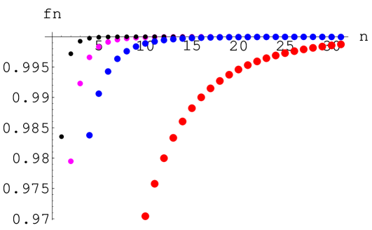
Figure 5: The coefficients $f_{n}$ in the Higgs field development for the $\Phi/2\pi=-1$ solutions (38) as a function of $n$ for different values of $\theta$. Size of dots decreases as $\theta\eta^{2}$ goes from $\theta\eta^{2}=0.1$ to $\theta\eta^{2}=0.9$.

5 Summary and discussion

In this paper we have examined vortex solutions in the Abelian Higgs model in non-commutative space, focussing on the properties of these solutions beyond the BPS point previously considered in [8], [11], [12], [15].

Previous to our investigations, the only known non-BPS solutions were fluxons [9], [11], negative flux solutions which are stable only for $\theta\eta^{2}>1$. These configurations, even though they are non-BPS in the sense that they do not satisfy the duality equations, share some properties with BPS solutions, namely, their energy saturates a topological bound and is linear in the flux. Moreover, in the $\theta\to 0$ commutative limite they correspond to singular configurations (with a $\delta$-function source).

We have constructed here non-BPS solutions of positive flux with arbitrary values $\theta\eta^{2}$ and also negative flux solutions, in this last case in the range $0\leq\theta\eta^{2}<1$. Unlike the fluxon case mentioned above, no simple analytical expressions of these solutions are available. One has instead expressions like eq.(31) so that the properties of the solutions have to be investigated numerically (as it happens in the commutative case, both for BPS and non-BPS solutions [24]-[23]).

The solutions presented here behave in most ways as smooth deformations of vortices in commutative space. For instance, their energy is an increasing function of $\lambda$ and is a linear function of the flux only at the BPS point. Indeed, we have shown that $E^{(M)}-ME^{(1)}>0$ for $\lambda>\lambda_{BPS}$ suggesting that in this case, the $M$-vortex configuration should be unstable towards the formation of a Abrikosov-type vortex lattice in analogy with Type II superconductors. Notice though that solutions in non-commutative space differ from solutions in ordinary space time as a result of parity breaking which manifests itself as a breaking of symmetry between vortex and anti-vortex configurations. We have illustrated this fact by comparing the energies of $E^{(1)}$ and $E^{(-1)}$ as a function of $\theta$.

Acknowledgements: We would like to thank D.Correa for helpful comments. E.F.M. would like to thanks the Physics Department of West Virginia University for the hospitality extended to him while part of this work was done. This work was partially supported by UNLP, UBA, CICBA, CONICET, ANPCYT (PICT grant 03-05179) Argentina and ECOS-Sud Argentina-France collaboration (grant A01E02). E.F.M. is partially supported by Fundación Antorchas, Argentina. GSL is partially supported by EPSRC grant GR/R70309.

References

• [1] J. A. Harvey, arXiv:hep-th/0102076.
• [2] M. R. Douglas and N. A. Nekrasov, Rev. Mod. Phys.  73 (2001) 977
• [3] R. J. Szabo, Phys. Rept.  378 (2003) 207.
• [4] N. Nekrasov and A. Schwarz, Commun. Math. Phys.  198 (1998) 689.
• [5] N. Seiberg and E. Witten, JHEP 9909 (1999) 032.
• [6] R. Gopakumar, S. Minwalla and A. Strominger, JHEP 0005 (2000) 020
• [7] D. J. Gross and N. A. Nekrasov, JHEP 0007 (2000) 034;D. J; JHEP 0103 (2001) 044
• [8] D. P. Jatkar, G. Mandal and S. R. Wadia, JHEP 0009 (2000) 018
• [9] A. P. Polychronakos, Phys. Lett. B 495 (2000) 407.
• [10] J. A. Harvey, P. Kraus and F. Larsen, JHEP 0012 (2000) 024
• [11] D. Bak, Phys. Lett. B 495 (2000) 251
• [12] G. S. Lozano, E. F. Moreno and F. A. Schaposnik, Phys. Lett. B 504 (2001) 117.
• [13] G. S. Lozano, E. F. Moreno and F. A. Schaposnik, JHEP 0102 (2001) 036.
• [14] A. Khare and M. B. Paranjape, JHEP 0104 (2001) 002.
• [15] D. Bak, K. M. Lee and J. H. Park, Phys. Rev. D 63 (2001) 125010.
• [16] K. Hashimoto and H. Ooguri, Phys. Rev. D 64 (2001) 106005
• [17] O. Lechtenfeld and A. D. Popov, JHEP 0111 (2001) 040
• [18] R. Gopakumar, M. Headrick and M. Spradlin, Commun. Math. Phys.  233 (2003) 355
• [19] F. Franco-Sollova and T. A. Ivanova, J. Phys. A 36 (2003) 4207
• [20] D. Tong, J. Math. Phys.  44 (2003) 3509
• [21] A. Hanany and D. Tong, JHEP 0307 (2003) 037
• [22] H. B. Nielsen and P. Olesen, Nucl. Phys. B 61 (1973) 45.
• [23] L. Jacobs and C. Rebbi, Phys. Rev. B 19 (1979) 4486.
• [24] H. J. de Vega and F. A. Schaposnik, Phys. Rev. D 14 (1976) 1100.