Properties of Chiral Wilson Loops.

Z. Guralnik^a and B. Kulik ^b

^a Institut für Physik

Humboldt-Universität zu Berlin

Newtonstraße 15

12489 Berlin, Germany

^b Max-Planck-Institut für Gravitationsphysik

Albert-Einstein-Institut

Am Mühlenberg 1, D-14476 Golm, Germany

Abstract

We study a class of Wilson Loops in ${\mathcal{N}}=4,D=4$ Yang-Mills theory belonging to the chiral ring of a ${\cal N}=2,d=1$ subalgebra. We show that the expectation value of these loops is independent of their shape. Using properties of the chiral ring, we also show that the expectation value is identically $1$. We find the same result for chiral loops in maximally supersymmetric Yang-Mills theory in three, five and six dimensions. In seven dimensions, a generalized Konishi anomaly gives an equation for chiral loops which closely resembles the loop equations of the three dimensional Chern-Simons theory.

1 Introduction

For a variety of reasons, it may be useful to write the action of a supersymmetric theory with D-dimensional Lorentz invariance in terms of a lower dimensional superspace. This procedure was developed originally in [1, 2] and has been helpful in extra-dimensional model building and in studying field theories of intersecting branes [3, 4, 5, 6]. Another application is the derivation of auxiliary k-dimensional bosonic matrix models which capture the holomorphic data of supersymmetric theories in $4+k$ dimensions [7, 8]. There is yet another possible use as a tool for obtaining non-renormalization theorems, but this has yet to be explored in much detail. The use of a lower dimensional superspace to obtain non- renormalization theorems was first hinted at in [3]. There it was used to suggest an alternative argument for the non-renormalization of the metric on the Higg’s branch of four-dimensional ${\cal N}=2$ gauge theories. This argument rests on the fact that some of the hypermultiplet kinetic terms arise from the superpotential in a lower dimensional superspace. In general, D-terms in theories with extended supersymmetry may become F-terms upon using a lower dimensional superspace. Furthermore gauge connections in directions transverse to the lower dimensional superspace may become components of chiral superfields. Thus holomorphic constraints may apply to quantities which one might not have expected.

In the subsequent discussion, we will use a lower dimensional superspace to obtain a non-renormalization theorem for BPS Wilson loops in maximally supersymmetric Yang-Mills theory in various dimensions. In particular, we will study the four dimensional ${\cal N}=4$ gauge theory using a ${\cal N}=2,d=1$ superspace. In this language, the superpotential is obtained from a Chern-Simons action by replacing gauge fields with chiral superfields. The diffeomorphism invariance of this superpotential leads to strong constraints on the chiral ring, defined with respect to ${\cal N}=2,d=1$ supersymmetry. We will focus on the equations satisfied by a class of Wilson loops belonging to the chiral ring.

Wilson loops in ${\mathcal{N}}=4$ gauge theory may involve the adjoint scalars and fermions as well as the gauge connections. Such Wilson loops have received considerable attention, beginning with [9]. In Euclidean space, the Wilson loop which is usually considered has the general form:

$$W_{\rm Euclidean}={\rm tr}P\exp i\int ds\left(A_{\mu}\frac{dx^{\mu}(s)}{ds}+iX^{m}\frac{dy^{m}(s)}{ds}\right)\,,$$ (1.1)

where $m=4\dots 9$. The path $x^{\mu}(s)$ must be closed for the Wilson loop to be gauge invariant, while no such constraint applies to the path $y^{m}(s)$. A special class of loops satisfying $\dot{y}^{2}=\dot{x}^{2}$ arises naturally in the context of minimal surfaces in $AdS$ [10, 11]. Loops in this class are at least locally BPS, which facilitates computation of the expectation value in some special cases such as the circular Wilson loop with fixed orientation in the $y^{m}$ directions [12, 13, 14]. This circular loop is annihilated by a linear combination of poincaré and special supersymmetries [14].

Wilson loops which are globally BPS with respect to the Poincaré supersymmetries were studied by Zarembo [15]. For these loops, $dy^{m}=dx^{\mu}M_{\mu}^{m}$, where the matrix satisfies:

$$M_{\mu}^{m}M_{\nu}^{m}=\delta_{\mu\nu}\,.$$ (1.2)

When these Wilson loops are extended in $\mathbb{R}^{2}$, $\mathbb{R}^{3}$ or $\mathbb{R}^{4}$ they are respectively $1/4,1/8$ or $1/16$ BPS. The Wilson loops which we will study have $y^{i+3}(s)=x^{i}(s)$ for $i=1,2,3$ with $x^{4}(s)={\rm const}$ and $y^{7,8,9}(s)=0$. These belong to the class of $1/4$ and $1/8$ BPS loops for which

$$M=\begin{pmatrix}1&0&0&0&0&0\cr 0&1&0&0&0&0\cr 0&0&1&0&0&0\cr 0&0&0&1&0&0\end{pmatrix}\,.$$ (1.3)

It turns out that these Wilson loops belong to the chiral ring of an ${\cal N}=2,d=1$ sub-algebra of the full ${\cal N}=4,D=4$ supersymmetry, and we will refer to them as “chiral Wilson loops”. Of course our results extend to any other loop related by the Lorentz and R-symmetries, which act in the obvious way on $M_{\mu}^{m}$.

To the first two orders in the ’t Hooft coupling and leading order in the $1/N$ expansion, it has been shown that all contributions to the expectation value of a globally BPS Wilson loop cancel [15], giving expectation value $1$. At large ’t Hooft coupling, AdS/CFT duality may be used to compute the expectation value of a Wilson loop [9, 11] by summing over minimal surfaces in AdS which are bounded by the loop. The minimal surfaces associated with the circular and rectangular BPS loops have zero regularized area [15], which together with a counting of zero modes leads to the expectation value $\exp(-A)=1$. On this basis, it was conjectured [15] that all $1/4$ BPS (planar) Wilson loops are non-renormalized.

By considering the equations of motion of the ${\mathcal{N}}=4$ theory in ${\mathcal{N}}=2,d=1$ superspace, we will obtain a loop equation showing that the expectation values of a chiral Wilson loop is independent of its shape. Together with properties of the chiral ring, this can be used to show that the expectation value is identically $1$. This holds whether the loop is $1/4$ BPS (planar) or $1/8$ BPS (extended in $\mathbb{R}^{3}$). This result is somewhat stronger than the conjecture of [15], which proposed non-renormalization of the $1/4$ BPS loops. The reason a stronger proposal was not made in [15] is the following. Besides the area of the minimal surface, the AdS computation of the loop expectation value also depends on the number of zero modes of the minimal surfaces. For loops in $\mathbb{R}^{3}$, a counting of the most transparent zero modes indicates a non-trivial dependence on the ’t Hooft coupling even if the regularized area is zero. However it is possible that there are other less obvious zero modes which were missed.

Our results concerning the non-renormalization of chiral Wilson loops in ${\mathcal{N}}=4$ Yang-Mills are easily extended to maximally supersymmetric Yang-Mills theory in dimensions $D=3,5$ and $6$ by using a four supercharge $d=D-3$ dimensional superspace. For $D=7$ however, we find a generalized Konishi anomaly which ruins the shape independence of the loop expectation value. The Konishi anomaly closely resembles the loop equations of three dimensional Chern-Simons theory. For dimensions $D>7$, our superspace formalism is no longer applicable.

2 $D$-dimensional maximally supersymmetric Yang-        Mills in $D-3$ dimensional superspace.

To obtain constraints on expectation values of certain BPS Wilson loops, we will make use of a formalism in which these loops manifestly belong to a chiral ring with respect to a lower dimensional supersymmetry algebra. In order to include gauge connections in chiral superfields, it is necessary to use a superspace with dimension less than that of the theory which one is studying. In this section, we will write the action of maximally supersymmetric D-dimensional Yang-Mills theory in terms of a four-supercharge $d=D-3$ dimensional superspace.

2.1 ${\cal N}=4$ SYM in quantum mechanical superspace

We wish to write the four-dimensional ${\cal N}=4$ SYM action in a one-dimensional ${\cal N}=2$ superspace. This is easily done by dimensional reduction of a result from the literature, in which 16-supercharge 7-dimensional Yang-Mills is written in terms of ${\cal N}=1,d=4$ superspace [2]. This superspace representation of the ${\mathcal{N}}=4$ theory was recently discussed in [6], where a relation between F and D-flatness and the calibration equations for a special Lagrangian manifold was demonstrated.

The one-dimensional ${\cal N}=2$ superspace resembles the familiar four dimensional ${\cal N}=1$ superspace, and can be obtained from it by dimensional reduction on $T^{3}$. We emphasize however that we are not dimensionally reducing the ${\cal N}=4$ theory, but writing the full four-dimensional action in terms of a one-dimensional superspace.

The ${\cal N}=2,d=1$ superfields entering the action for the four-dimensional ${\cal N}=4$ Yang-Mills theory have the general form $F(t,\theta,\bar{\theta}|\vec{x})$, where $(t,\theta,\bar{\theta})$ spans the one dimensional superspace, and $\vec{x}\sim(x^{1},x^{2},x^{3})$ can be regarded as continuous indices. The necessary degrees of freedom are contained in three chiral fields $\Phi_{i}$ and a vector field $V$. The vector superfield satisfies $V=V^{\dagger}$. Chiral superfields $\Phi$ satisfy $\bar{D}_{\alpha}\Phi=0$, where:

$$\bar{D}_{\alpha}=-\frac{\partial}{\partial\bar{\theta}^{\alpha}}-i\theta^{\alpha}\partial_{t}\,\qquad D_{\alpha}=-\frac{\partial}{\partial\theta^{\alpha}}-i\bar{\theta}^{\alpha}\partial_{t}\,.$$ (2.4)

The index $\alpha=1,2$ is associated with the $SU(2)$ R-symmetry of ${\mathcal{N}}=2,d=1$. The action of the four dimensional ${\cal N}=4$ theory in ${\cal N}=2,d=1$ superspace is:

$$S= \frac{1}{g^{2}}\int d^{3}x\,dt\,\left.{\rm tr}\,\left[{\cal W}_{\alpha}{\cal W}^{\alpha}+\epsilon_{ijk}(\Phi_{i}\frac{\partial}{\partial x^{j}}\Phi_{k}+\frac{2}{3}i\Phi_{i}\Phi_{j}\Phi_{k})\right]\right|_{\theta\theta}+cc\,+$$

$$\frac{1}{g^{2}}\left.\int d^{3}x\,dt\,{\rm tr}\,\bar{\Omega}_{i}e^{V}\Omega_{i}e^{-V}\right|_{\theta\theta\bar{\theta}\bar{\theta}}\,,$$ (2.5)

where the indices $i,j,k$ take values from $1$ to $3$, $W_{\alpha}=\bar{D}\bar{D}e^{V}D_{\alpha}e^{-V}$, and:

$$\Omega_{i}\equiv\Phi_{i}+e^{-V}(i\partial_{i}-\bar{\Phi}_{i})e^{V}\,.$$ (2.6)

Although the superfield content of the ${\cal N}=4$ theory in ${\cal N}=2,d=1$ superspace is similar to that in ${\cal N}=1,d=4$ superspace, the component fields are distributed very differently. The bosonic fields of the ${\mathcal{N}}=4$ theory consist of four components of the gauge connections $A_{0,1,2,3}$ and six Hermitian adjoint scalars $X_{4,5,6,7,8,9}$. These are distributed amongst the ${\mathcal{N}}=2,d=1$ superfields $V$ and $\Phi_{i}$ as follows:

$$V\rightarrow A_{0},X^{7,8,9}\qquad\Phi_{i}\rightarrow A_{i},X^{i+3}\,.$$ (2.7)

The combination $A_{i}+iX^{i+3}$ is the bottom component of the chiral super-field $\Phi_{i}$. Gauge transformations are parameterized by ${\cal N}=2,d=1$ chiral superfields $\Lambda(t,\theta;\vec{x})$ which act in the following way:

$$e^{V} \rightarrow e^{i\Lambda^{\dagger}}e^{V}e^{-i\Lambda}$$ (2.8)

$$\Phi_{i} \rightarrow e^{i\Lambda}\Phi_{i}e^{-i\Lambda}-e^{i\Lambda}i\frac{\partial}{\partial x^{i}}e^{-i\Lambda}\,,$$ (2.9)

under which:

$$\Omega_{i}\rightarrow e^{i\Lambda}\Omega_{i}e^{-i\Lambda}\,.$$ (2.10)

Four dimensional Lorentz invariance is not manifest, but becomes apparent upon integrating out F and D-terms.

Note that the superpotential resembles a Chern-Simons action and is diffeomorphism invariant, although the theory as a whole is not. We shall take advantage of this feature to obtain information about a class of Wilson Loops which are chiral with respect to the one dimensional ${\cal N}=2$ supersymmetry algebra.

2.2 Euclidean action

One can also write the Euclidean ${\mathcal{N}}=4,D=4$ action in one dimensional superspace. To this end, we start with the Minkowski-space action for a D6-brane (7-dimensional maximally supersymmetric Yang-Mills), which in four-dimensional ${\mathcal{N}}=1$ superspace is:

$$S= \frac{1}{g^{2}}\int d^{3}x\,d^{4}y\,\left.{\rm tr}\,\left[{\cal W}_{\alpha}{\cal W}^{\alpha}+\epsilon_{ijk}(\Phi_{i}\frac{\partial}{\partial x^{j}}\Phi_{k}+\frac{2}{3}i\Phi_{i}\Phi_{j}\Phi_{k})\right]\right|_{\theta\theta}+cc.+$$ (2.11)

$$\frac{1}{g^{2}}\left.\int d^{3}x\,d^{4}y\,{\rm tr}\,\bar{\Omega}_{i}e^{V}\Omega_{i}e^{-V}\right|_{\theta\theta\bar{\theta}\bar{\theta}}\,.$$ (2.12)

Compactifying the time direction $y^{0}$ and two spatial directions $y^{1},y^{2}$ belonging to the four dimensional superspace gives an action of the same form as (2.1), the only difference coming from the definition of the operators $D_{\alpha}$ and.$\bar{D}_{\alpha}$. Note that the R-symmetry associated with the four-dimensional Euclidean ${\mathcal{N}}=4$ supergroup is $Spin(1,5)$. Non-compact R-symmetry groups are a well known feature of Euclidean theories with extended supersymmetry. For a discussion of Euclidean supersymmetry see [16, 17, 18, 19, 20, 21].

2.3 Other dimensions

The above discussion is readily generalized to maximally supersymmetric Yang-Mills theories in $D=3,5,6$ and $7$ dimensions. In a four supercharge $d=D-3$ dimensional superspace, the action of the theory is just:

$$S= \frac{1}{g^{2}}\int d^{3}x\,d^{d}y\,\left.{\rm tr}\,\left[{\cal W}_{\alpha}{\cal W}^{\alpha}+\epsilon_{ijk}(\Phi_{i}\frac{\partial}{\partial x^{j}}\Phi_{k}+\frac{2}{3}i\Phi_{i}\Phi_{j}\Phi_{k})\right]\right|_{\theta\theta}+cc.+$$ (2.13)

$$\frac{1}{g^{2}}\left.\int d^{3}x\,d^{d}y\,{\rm tr}\,\bar{\Omega}_{i}e^{V}\Omega_{i}e^{-V}\right|_{\theta\theta\bar{\theta}\bar{\theta}}\,.$$ (2.14)

Note that for $d=0$, the action can be viewed as that of a supersymmetric matrix model, with an infinite number of matrix superfields labelled by $\vec{x}$. The supersymmetry generators are:

$$Q_{\alpha}=\frac{\partial}{\partial\theta^{\alpha}},\qquad\bar{Q}_{\alpha}=\frac{\partial}{\partial\bar{\theta}^{\alpha}}\,.$$ (2.15)

Chiral superfields $\Phi$ are defined by $\bar{D}_{\alpha}\Phi=0$, where:

$$D_{\alpha}=\frac{\partial}{\partial\theta^{\alpha}},\qquad\bar{D}_{\alpha}=\frac{\partial}{\partial\bar{\theta}^{\alpha}}\,,$$ (2.16)

such that $\Phi=\phi+\theta\psi+\theta\theta F$. Vector superfields are defined as usual by $V=\bar{V}$. The three gauge connections and seven adjoint scalars of the theory are distributed amongst these superfields as follows:

$$V\rightarrow X^{7,8,9,10},\qquad\Phi_{i}\rightarrow A_{i},X^{i+3}\,,$$ (2.17)

where $i=1,2,3$. As always, three of the gauge connections belong to the lowest component of chiral superfields. Upon integrating out auxiliary fields, one finds the Euclidean action of the maximally supersymmetric $D=3$ Yang-Mills theory . It should be noted that for the zero dimensional superspace there is no chiral ring in the usual sense. The expectation value of a product of chiral operators is not necessarily the product of the expectation values. Since the superspace is $0$ dimensional, one can not make the usual cluster property argument to show that the expectation value of the product is the product of the expectation values.

3 Chiral Loop equations

Consider the variation:

$$\Phi_{i}(\vec{x})\rightarrow\Phi_{i}(\vec{x})+\epsilon g_{i,\vec{x}}[\Phi]\,,$$ (3.18)

where $\epsilon$ is a chiral function and $g_{I,\vec{x}}$ is, for the moment, an arbitrary functional of chiral superfields. The equations of motion which follow from this variation are:

$$\bar{D}^{2}\,{\rm tr}\,\left(g_{i,\vec{x}}[\Phi](e^{-V(\vec{x})}\bar{\Omega}_{i}(\vec{x})e^{V(\vec{x})}-\Omega_{i}(\vec{x}))\right)+{\rm tr}\,g_{i,\vec{x}}[\Phi]\frac{\delta W}{\delta\Phi_{i}(\vec{x})}={\cal A}\,.$$ (3.19)

where ${\cal A}$ is a possible anomalous term which vanishes classically. Since $\Phi_{i}|_{\theta=\bar{\theta}=0}$ contains the spatial gauge connections, let us choose $g_{i,\vec{x}}[\Phi]$ to be a spatial Wilson line on a contour ${\cal C}$ which begins and ends at the point $\vec{x}$:

$$g_{i,\vec{x}}[\Phi]=W(C,\vec{x})=P\exp\left(i\int_{{\cal C},\vec{x}}^{\vec{x}}\vec{\Phi}\cdot d\vec{y}\right)\,.$$ (3.20)

With this choice equation (3.19) becomes:

$$\bar{D}^{2}(\cdots)={\rm tr}\left(W(C,\vec{x})\epsilon_{ijk}{\cal F}_{jk}(\vec{x})\right)+{\cal A}\,,$$ (3.21)

where:

$${\cal F}_{jk}=\partial_{j}\Phi_{k}-\partial_{k}\Phi_{j}+i[\Phi_{j},\Phi_{k}]\,.$$ (3.22)

In the next section, we shall argue that the anomaly vanishes, so long as we are considering maximally supersymmetric Yang-Mills in less than 7 dimensions.

The relation $(\bar{D}^{2}J)|_{\theta=\bar{\theta}=0}=[\bar{Q},[\bar{Q},J|_{\theta=\bar{\theta}=0}]$ holds for any gauge invariant superfield $J$, such that $\langle\bar{D}^{2}J|_{\theta=\bar{\theta}=0}\rangle=0$ in a supersymmetric vacuum. Therefore (3.21) implies:

$$\left<\left.{\rm tr}\left(W(C,\vec{x})\epsilon_{ijk}{\cal F}_{jk}(\vec{x})\right)\right|_{\theta=\bar{\theta}=0}\right>=\langle{\cal A}|_{\theta=\bar{\theta}=0}\rangle\,.$$ (3.23)

The insertion of the field strength ${\cal F}_{jk}$ generates an infinitesimal deformation of the contour ${\cal C}$ in the $jk$ plane (see figure 1.).

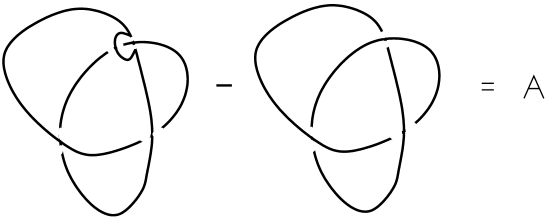
Figure 1: (Almost) loop equation.

If the anomaly vanishes, the chiral Wilson loops have no dependence on their shape. This is a much stronger statement than diffeomorphism invariance, since the expectation value does not even have any dependence on the loop topology. Note that there are no terms in the loop equation which contribute when segments of the loop cross each other. There should be no ambiguities in defining the expectation values of self intersecting Wilson loops.

Shape independence implies that the expectation value of the chiral Wilson loop can only be a function of the gauge coupling and theta angle in the conformal four dimensional case. In dimensions other than four, shape independence implies that the expectation value is a number. This number can be shown to be $1$ by taking a weak coupling limit, corresponding to shrinking the loop in three dimensions and expanding the loop in five and more dimensions. In seven dimensions, we will argue that the anomaly is non-zero.

In the conformal four dimensional case, shrinking the loop is ill defined since there is no scale in the theory. One might try to show that the expectation value is still $1$ by using “zig-zag” symmetry. Zig-zag symmetry means that segments of a loop which backtrack cancel each other. This has been emphasized as a basic property of the QCD string [22], for which one only considers loops involving the gauge field, but is not necessarily a property of Wilson loops such as (1.1) which also involve the scalar fields. The chiral Wilson loops satisfy zig-zag symmetry because of the equivalence of the paths associated with the gauge field and the scalars. Assuming that shape independence includes singular deformations of the loop, zig-zag symmetry implies:

$$\left<\frac{1}{N}{\rm tr}P\exp\left(i\oint_{\Sigma\in\mathbb{R}^{2}}\phi\right)\right>=1\,,$$ (3.24)

through the manipulations illustrated in figure 2. Note however that this requires the introduction of a cusp.

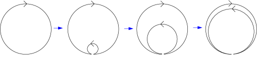
Figure 2: Using zig-zag symmetry and shape independence to show that $\langle\frac{1}{N}{\rm}trW(C)\rangle=1$. This assumes that shape independence still holds when cusps are introduced. An argument which avoids this assumption relies on properties of the chiral ring.

Fortunately, there is another argument that the expectation value is one, which does not require passing through a loop with a cusp. Given a Wilson-loop $\frac{1}{N}{\rm tr}W$ associated with a path C in $\mathbb{R}^{3}$ one can smoothly deform the path within $\mathbb{R}^{3}$ such that it goes around $C$ multiple times and the Wilson loop becomes $\frac{1}{N}{\rm tr}W^{n}$ for any $n>1$. Shape independence implies that the expectation value is unchanged:

$$\langle\frac{1}{N}{\rm tr}W^{n}\rangle=\langle\frac{1}{N}{\rm tr}W\rangle\,.$$ (3.25)

Furthermore, there are relations amongst the variables ${\rm tr}W^{n}$, such that ${\rm tr}W^{n}$ for $n=1\cdots 2N^{2}$ form a complete independent set. Since the chiral Wilson loops belong to a chiral ring, the expectation values factorize:

$$\langle\frac{1}{N}{\rm tr}W^{n}\frac{1}{N}{\rm tr}W^{m}\rangle=\langle\frac{1}{N}{\rm tr}W^{n}\rangle\langle\frac{1}{N}{\rm tr}W^{m}\rangle\,.$$ (3.26)

The relations amongst the $\frac{1}{N}{\rm tr}W^{n}$, together with (3.26) and (3.25) are solved by:

$$\langle\frac{1}{N}{\rm tr}W^{n}\rangle=\frac{1}{N}{\rm tr}{\cal W}_{c}\,,$$ (3.27)

where ${\cal W}_{c}$ is a matrix (analogous to a master field) satisfying ${\cal W}_{c}^{2}={\cal W}_{c}$. In the weak coupling limit ${\cal W}_{c}=I$. Assuming that the expectation value of the Wilson loop depends smoothly on the coupling one has ${\cal W}_{c}=I$ for any coupling, so that and $\langle\frac{1}{N}{\rm tr}W\rangle=1$.

Note that in the four dimensional ${\cal N}=4$ theory, the expectation value of the chiral Wilson loops is identically $1$ to at least the first two orders in the ’t Hooft coupling and leading order in $1/N$ [15]. This is essentially due to cancellations between greens functions of $A_{i}$ and $X^{i+3}$ due to the relative factor of $i$ in the exponent of the Wilson loop, $\phi_{i}=A_{i}+iX^{i+3}$.

3.1 Variation of the functional measure.

To see if there is a non-zero anomaly ${\mathcal{A}}$ in (3.21), we will compute the variation of the functional measure under (3.18) using methods discussed in [23, 24]. The Jacobian is formally:

$$J=\left|{\rm det}_{c}\frac{\delta\Phi_{i}^{\prime}(Z^{\prime})}{\delta\Phi_{j}(Z)}\right|\,,$$ (3.28)

where $Z$ collectively denotes the superspace coordinates $z\sim\vec{y},\theta,\bar{\theta}$ and the transverse spatial coordinates $\vec{x}$. The subscript “c” in ${\rm det}_{c}$ stands for chiral part of the whole super-determinant. It will be convenient to define a Hilbert space spanned by $|Z,A\rangle$, which is a complete set of states in a superspace coordinate representation satisfying:

$$\hat{Z}|Z,A\rangle=Z|Z,A\rangle,\qquad\hat{T}^{A}|Z,B\rangle=f_{ABC}|Z,C\rangle$$

$$\langle Z,A|Z^{\prime},B\rangle\ =\delta_{AB}\delta^{3}(\vec{x}-\vec{x}^{\prime})\delta^{d}(y-y^{\prime})\delta^{4}(\theta-\theta^{\prime}),$$ (3.29)

where $\hat{T}^{A}$ are $U(N)$ generators and $f_{ABC}$ are the $U(N)$ structure functions. We can then write:

$$\frac{\delta\Phi_{i}^{A}(Z^{\prime})}{\delta\Phi_{j}^{B}(Z)}=\delta_{ij}\delta_{AB}\delta^{3}(\vec{x}-\vec{x}^{\prime})\delta^{d}(y-y^{\prime})\delta^{2}(\theta-\theta^{\prime})=<Z,A|\bar{D}^{2}|Z^{\prime},B>\,.$$ (3.30)

For the infinitesimal variation (3.18), the Jacobian is:

$$J=1+{\rm tr}_{c}\,\epsilon\bar{D}^{2}\frac{\delta g_{i,\vec{x}}}{\delta\Phi_{i}(\vec{x})}=\int dZ_{c}\,\sum_{A}\,\epsilon(Z)\langle Z,A|\bar{D}^{2}\frac{\delta g^{i}[\Phi]}{\delta\Phi^{i}}|Z,A\rangle\,,$$ (3.31)

where $dZ_{c}$ is the chiral measure $d^{d}y\,d^{2}\theta\,d^{3}x$. The matrix:

$$\langle Z,A|\frac{\delta g_{i,\vec{x}}[\Phi]}{\delta\Phi_{i}(\vec{x}^{\prime})}(-\bar{D}^{2}/4)|Z^{\prime}A>\,,$$ (3.32)

is proportional to $\delta^{2}(\theta-\theta^{\prime})=(\theta-\theta^{\prime})^{2}$ and so has vanishing diagonal entries. Thus naively $J=1$. However this is not necessarily true upon regularizing the trace.

To obtain the Jacobian for the transformation $\Phi^{i}\rightarrow\Phi^{i}+\epsilon g^{i}[\Phi]$, we need to regularize the diagonal elements of the matrix (3.32):

$${\cal M}_{\vec{x},z,A}\equiv\,<\vec{x},z,A|\bar{D}^{2}\frac{\delta g^{i}[\Phi]}{\delta\Phi^{i}}|\vec{x},z,A>\,.$$ (3.33)

In the more familiar context of the Konishi anomaly in ${\mathcal{N}}=1$ four dimensional gauge theory, this is accomplished [23] by the insertion of an operator $\exp(-\hat{L}/M^{2})$ where:

$$\hat{L}\equiv-\frac{1}{16}\bar{D}^{2}e^{-V}D^{2}e^{V}\,.$$ (3.34)

Note that this operator is gauge covariant and chiral. However, the insertion of $\exp(-\hat{L}/M^{2})$ will not suffice in our case, since this only cuts off large momenta in directions belonging to the superspace, which is lower-dimensional in our case. The regularized version of (3.33) which we will consider is:

$${\cal M}_{\vec{x},z,A}\equiv\,<\vec{x},z,A|\exp(-\hat{\cal L}/M^{2})\,\bar{D}^{2}\,\frac{\delta g^{i}[\Phi]}{\delta\Phi^{i}}|\vec{x},z,A>\,,$$ (3.35)

where:

$$\hat{\cal L}=\hat{L}+(\partial_{i}+\Phi_{i})(\partial_{i}+\Phi_{i})\,.$$ (3.36)

To evaluate (3.35), note that:

$$\hat{L}(\bar{D}^{2}\cdots)=(\partial_{t}^{2}-{1/2}{\cal W}^{\alpha}D_{\alpha}+C\partial_{t}+F)(\bar{D}^{2}\cdots)\,,$$ (3.37)

where:

$$C\equiv\frac{1}{2}\bar{D}_{\alpha}e^{-V}\bar{D}_{\alpha}e^{V}$$

$$F\equiv\frac{1}{16}\bar{D}^{2}e^{-V}D^{2}e^{V}\,.$$ (3.38)

We can write:

$$e^{-{\cal L}/M^{2}}=e^{-\nabla/M^{2}}\hat{\cal S}\,,$$ (3.39)

where $\nabla$ is the Laplacian in the space including all bosonic coordinates, $\nabla\equiv\nabla_{\vec{x}}^{2}+\nabla_{\vec{y}}^{2}$  . The factor $\hat{\cal S}=1+\dots$ must contain a term with two $D_{\alpha}$ operators for $\exp(\hat{\cal L}/M^{2})\bar{D}^{2}$ to give a non-zero contribution to (3.35). To illustrate this property, note that:

$$<z^{\prime}|D^{2}\bar{D}^{2}|z> =\delta^{d}(y-y^{\prime})D^{2}\bar{D}^{2}\delta^{2}(\theta-\theta^{\prime})\delta^{2}(\bar{\theta}-\bar{\theta}^{\prime})$$

$$=\delta^{d}(y-y^{\prime})D^{2}\bar{D}^{2}(\theta-\theta^{\prime})^{2}(\bar{\theta}-\bar{\theta}^{\prime})^{2}=\delta^{d}(y-y^{\prime})\,.$$ (3.40)

If the $D^{2}$ were removed, the diagonal matrix element would vanish. Thus, (3.37) implies that, in a large $M^{2}$ expansion, the leading non-zero contribution to (3.35) is:

$${\cal M}_{\vec{x},z,A}=$$

$$<\vec{x},z,A|\exp(-\nabla/M^{2})\frac{W_{\alpha}W^{\alpha}}{M^{4}}D^{2}\bar{D}^{2}|\vec{x}^{\prime},z^{\prime},A^{\prime}><\vec{x}^{\prime},z^{\prime},A^{\prime}|\frac{\delta g^{i}}{\delta\Phi^{i}}|\vec{x},z,A>+\cdots\,,$$ (3.41)

where the summation over primed variables is assumed and:

$$<\vec{x}^{\prime},z^{\prime},A^{\prime}|\frac{\delta g^{i}}{\delta\Phi^{i}}|\vec{x},z,A>\equiv\,\frac{\delta g^{i}_{\vec{x}^{\prime},A^{\prime}}}{\delta\Phi^{i}_{\vec{x},A}}\delta^{d}(\vec{y}^{\prime}-\vec{y})\delta^{2}(\theta-\theta^{\prime})\delta^{2}(\bar{\theta}^{\prime}-\bar{\theta})\,.$$ (3.42)

Expression (3.1) can be evaluated by inserting the identity $|k_{x},k_{y},C><k_{x},k_{y},C|$   after $\exp(-\nabla/M^{2})$, where $|k_{x},k_{y},C>$ is an eigenvector of the momentum operators in the transverse space $\vec{x}$ and the bosonic part of the superspace $z$. The result is:

$${\cal M}_{\vec{x},z,A}=\qquad\qquad\qquad\qquad\qquad\qquad\qquad\qquad\qquad\qquad\qquad\qquad$$

$$\int d^{3}k_{x}\,d^{d}k_{y}\,d^{3}x^{\prime}\,d^{d}y^{\prime}\,\exp\left(-\frac{\vec{k}_{x}^{2}+\vec{k}_{y}^{2}}{M^{2}}+i\vec{k}_{x}\cdot(\vec{x}-\vec{x}^{\prime})+i\vec{k}_{y}\cdot(\vec{y}-\vec{y}^{\prime})\right)$$

$$\frac{1}{M^{4}}W_{\alpha}^{D}(\vec{x}^{\prime},z^{\prime})W^{\alpha E}(\vec{x}^{\prime},z^{\prime})<A|\hat{T}^{D}\hat{T}^{E}|A^{\prime}>\frac{\delta g^{i}_{\vec{x}^{\prime},A^{\prime}}}{\delta\Phi^{i}_{\vec{x},A}}\delta^{d}(\vec{y}^{\prime}-\vec{y})+\cdots$$

$$=M^{d-4}W_{\alpha}^{D}(\vec{x},z)W^{\alpha E}(\vec{x},z)<A|\hat{T}^{D}\hat{T}^{E}|A^{\prime}>\frac{\delta g^{i}_{\vec{x},A^{\prime}}}{\delta\Phi^{i}_{\vec{x},A}}+\cdots$$

$$=M^{d-4}\sum_{I,J}\left[{\cal W}^{\alpha}(\vec{x}),\left[{\cal W}_{\alpha}(\vec{x}),\frac{\delta g_{i,\vec{x}}[\Phi]}{\delta{\Phi_{i}(\vec{x})}_{IJ}}\right]\right]_{IJ}+\cdots\,,$$ (3.43)

where “$\cdots$” indicates sub-leading terms in $1/M$. The indices $I$ and $J$ in the last line are $N\times N$ matrix indices. After sending the regularization mass $M$ to infinity the anomaly vanishes for $d<4$, corresponding to the maximally supersymmetric Yang-Mills theory in dimensions $D<7$. For $D=7$ one has:

$$\left<\left.{\rm tr}\left(W(C,\vec{x})\epsilon_{ijk}{\cal F}_{jk}(\vec{x})\right)\right|_{\theta=\bar{\theta}=0}\right>=\left<\left.\sum_{I,J}\left[{\cal W}^{\alpha}(\vec{x}),\left[{\cal W}_{\alpha}(\vec{x}),\frac{\delta W(C,\vec{x})}{\delta{\Phi_{i}(\vec{x})}_{IJ}}\right]\right]_{IJ}\right|_{\theta=\bar{\theta}=0}\right>\,.$$ (3.44)

Due to the anomaly on the right hand side of (3.44), this is not quite an equation in loop space, although it does closely resemble the loop equation for a three-dimensional Chern-Simons theory, which very formally follows from:

$$0=\int DA\frac{\delta}{\delta A^{a}_{i}(\vec{x})}\left(g^{a}_{i,\vec{x}}[A]e^{-S_{CS}}\right)\,.$$ (3.45)

If $g_{i,\vec{x}}=W(C,\vec{x})$ is chosen to be a Wilson loop with a marked point, (3.45) becomes:

$$\frac{k}{4\pi}\left<{\rm tr}W(C,\vec{x})\epsilon_{ijk}F_{jk}(\vec{x})\right>=\left<\left.\sum_{I,J}\frac{\delta W(C,\vec{x})}{\delta{\Phi_{i}(\vec{x})}_{IJ}}\right|_{IJ}\right>\,.$$ (3.46)

Regularizing and making sense of such equations to obtain the so called Skein relations is non-trivial [25].

The fact that an anomaly in the loop equations appears only in 7-dimensions, for which our construction involves ${\cal N}=1,d=4$ superspace, is consistent with recent conjectures of Dijkgraff and Vafa. A generalized Konishi anomaly is known to be crucial for the gauge theory derivation [24] of the Dijkgraff-Vafa proposal [26, 27] relating the holomorphic data of ${\cal N}=1,D=4$ gauge theories to large $N$ bosonic matrix models. This proposal was extended in [7] to the case of $D=4+n$ dimensional theories preserving (at least) ${\cal N}=1,d=4$ supersymmetry. In this case the holomorphic data was conjectured to be captured by an auxiliary $n$ dimensional bosonic gauge theory. The action of this auxiliary gauge theory corresponds to the superpotential of the $4+n$ dimensional theory written in four dimensional ${\cal N}=1$ superspace. For the case of the supersymmetric gauge theory describing a D6-brane wrapping a three-cycle of a Calabi-Yau, the auxiliary bosonic gauge theory is Chern-Simons theory on the three-cycle. Proving the validity of the proposal of [7] by field theoretic methods (as in [24]) would presumably require a non-trivial Konishi anomaly, which we have found above. It would be very interesting if one could find a generalization of the chiral Wilson loops for which the loop equations more closely resemble those of the large $N$ Chern-Simons theory.

There is a possibly important subtlety in the above discussion, which is that (3.18) includes a variation of the gauge fields. In practice, one must fix the gauge via a Faddeev-Popov procedure to define the functional measure. This amounts to introducing ghosts and extra terms in the action. We have computed the variation of the functional measure without gauge fixing so that our result appears somewhat formal. However we have also chosen $g_{i,\vec{x}}$ so as to get equations involving gauge invariant operators. The extra terms in the action do not effect the classical equations for these operators. Furthermore the anomalous term arises from the variation of a part of the functional measure which does not involve ghosts. Thus we expect that the anomaly equation is insensitive to the gauge fixing. .

4 Conclusions and Remarks

We have obtained a non-renormalization theorem for a class of Wilson loops in maximally supersymmetric Yang-Mills in dimensions $D=3,4,5$ and $6$. We have made use of the fact that these Wilson loops belong to the chiral ring associated with a D-3 dimensional sub-algebra of the full supersymmetry. A non-renormalization theorem for these loops was conjectured previously by Zarembo [15] in the case of a planar path. We find a stronger result which includes chiral loops in $\mathbb{R}^{3}$. It would be very interesting to understand the stronger result from the AdS point of view, where it has not been shown in general that chiral loops are boundaries of minimal surfaces with zero regularized area. In fact this has only been demonstrated for circular and infinitely long rectangular loops.

The results of this article persist upon taking the three world-volume dimensions transverse to the d=D-3 dimensional superspace to be a curved space (such as a special Lagrangian inside a Calabi-Yau three-fold). Generically, this leaves a theory preserving only four supercharges in D-3 dimensions. Our results are unchanged due to the diffeomorphism invariance of the Chern-Simons superpotential. The non-diffeomorphism invariant parts of the action contribute terms of the form $\bar{D}^{2}(\cdots)$ in the equations of motion for chiral loops. Supersymmetry implies that such terms vanish upon taking the expectation value.

We emphasize that in various instances, gauge fields may be manifestly included in chiral operators by making use of a lower dimensional superspace. This may have interesting applications besides the one which we have presented.

5 Acknowledgements

The authors wish to thank L. Alvarez-Gaumé, J. Erdmenger, I. Kirsch, S. Kovacs, D. Lüst, N. Prezas and K. Zarembo for enlightening discussions. The work of Z.G. is funded by the DFG (Deutsche Forschungsgemeinschaft) within the Emmy Noether programme, grant ER301/1-2. The work of BK is supported by German-Israeli-Foundation, GIF grant I-645-130.14/1999

References

- [1] N. Marcus, A. Sagnotti and W. Siegel, “Ten-Dimensional Supersymmetric Yang-Mills Theory In Terms Of Four-Dimensional Superfields,” Nucl. Phys. B 224, 159 (1983).
- [2] N. Arkani-Hamed, T. Gregoire and J. Wacker, “Higher dimensional supersymmetry in 4D superspace,” JHEP 0203, 055 (2002) [arXiv:hep-th/0101233].
- [3] J. Erdmenger, Z. Guralnik and I. Kirsch, “Four-dimensional superconformal theories with interacting boundaries or defects,” Phys. Rev. D 66, 025020 (2002) [arXiv:hep-th/0203020].
- [4] N. R. Constable, J. Erdmenger, Z. Guralnik and I. Kirsch, “Intersecting D3-branes and holography,” arXiv:hep-th/0211222.
- [5] N. R. Constable, J. Erdmenger, Z. Guralnik and I. Kirsch, “(De)constructing intersecting M5-branes,” Phys. Rev. D 67, 106005 (2003) [arXiv:hep-th/0212136].
- [6] J. Erdmenger, Z. Guralnik, R. Helling and I. Kirsch, hep-th/0309043.
- [7] R. Dijkgraaf and C. Vafa, “N = 1 supersymmetry, deconstruction, and bosonic gauge theories,” arXiv:hep-th/0302011.
- [8] I. Bena and R. Roiban, “N = 1* in 5 dimensions: Dijkgraaf-Vafa meets Polchinski-Strassler,” arXiv:hep-th/0308013.
-
[9]
J. M. Maldacena, “Wilson loops in large N field theories,”
Phys. Rev. Lett. 80, 4859 (1998) [arXiv:hep-th/9803002];
Soo-Jong Rey, Jung-Tay Yee, “Macroscopic strings as heavy quarks: Large-N gauge theory and anti-de Sitter supergravity”, Eur.Phys.J.C22:379-394 (2001) [arXive:hep-th/9803001];
Soo-Jong Rey, S. Theisen, Jang-Tay Yee, “Wilson-Polyakov Loop at Finite Temperature in Large N Gauge Theory and Anti-de Sitter Supergravity”, Nucl.Phys. B527:171-186 (1998) [arXive: hep-th/9803135]. - [10] D. Berenstein, R. Corrado, W. Fischler, J. Maldacena, “The Operator Product Expansion for Wilson Loops and Surfaces in the Large N Limit”, Phys. Rev. D 59,105023 (1999) [arXiv:hep-th/9809188].
- [11] N. Drukker, D. J. Gross and H. Ooguri, “Wilson loops and minimal surfaces,” Phys. Rev. D 60, 125006 (1999) [arXiv:hep-th/9904191].
- [12] J. K. Erickson, G. W. Semenoff and K. Zarembo, “Wilson loops in N = 4 supersymmetric Yang-Mills theory,” Nucl. Phys. B 582, 155 (2000) [arXiv:hep-th/0003055].
- [13] N. Drukker and D. J. Gross, “An exact prediction of N = 4 SUSYM theory for string theory,” J. Math. Phys. 42, 2896 (2001) [arXiv:hep-th/0010274].
- [14] M. Bianchi, M. B. Green and S. Kovacs, “Instanton corrections to circular Wilson loops in N = 4 supersymmetric Yang-Mills,” JHEP 0204, 040 (2002) [arXiv:hep-th/0202003].
- [15] K. Zarembo, “Supersymmetric Wilson loops,” Nucl. Phys. B 643, 157 (2002) [arXiv:hep-th/0205160].
- [16] B. Zumino, “Euclidean Supersymmetry And The Many-Instanton Problem,” Phys. Lett. B 69, 369 (1977).
- [17] P. van Nieuwenhuizen and A. Waldron, “On Euclidean spinors and Wick rotations,” Phys. Lett. B 389, 29 (1996) [arXiv:hep-th/9608174].
- [18] P. van Nieuwenhuizen and A. Waldron, “A continuous Wick rotation for spinor fields and supersymmetry in Euclidean space,” arXiv:hep-th/9611043.
- [19] M. Blau and G. Thompson, “Euclidean SYM theories by time reduction and special holonomy manifolds,” Phys. Lett. B 415, 242 (1997) [arXiv:hep-th/9706225].
- [20] A. V. Belitsky, S. Vandoren and P. van Nieuwenhuizen, “Instantons, Euclidean supersymmetry and Wick rotations,” Phys. Lett. B 477, 335 (2000) [arXiv:hep-th/0001010].
- [21] U. Theis and P. Van Nieuwenhuizen, “Ward identities for N = 2 rigid and local supersymmetry in Euclidean space,” Class. Quant. Grav. 18, 5469 (2001) [arXiv:hep-th/0108204].
- [22] A. M. Polyakov, “String theory and quark confinement,” Nucl. Phys. Proc. Suppl. 68, 1 (1998) [arXiv:hep-th/9711002].
- [23] K. i. Konishi and K. i. Shizuya, “Functional Integral Approach To Chiral Anomalies In Supersymmetric Gauge Theories,” Nuovo Cim. A 90, 111 (1985).
- [24] F. Cachazo, M. R. Douglas, N. Seiberg and E. Witten, “Chiral rings and anomalies in supersymmetric gauge theory,” JHEP 0212, 071 (2002) [arXiv:hep-th/0211170].
- [25] R. Gambini and J. Pullin, “Variational derivation of exact skein relations from Chern–Simons theories,” Commun. Math. Phys. 185, 621 (1997) [arXiv:hep-th/9602165].
- [26] R. Dijkgraaf and C. Vafa, “A perturbative window into non-perturbative physics,” arXiv:hep-th/0208048.
- [27] R. Dijkgraaf and C. Vafa, “Matrix models, topological strings, and supersymmetric gauge theories,” Nucl. Phys. B 644, 3 (2002) [arXiv:hep-th/0206255].