hep-th/0309116

New Phase Diagram for

Black Holes and Strings on Cylinders

Troels Harmark^a,b and Niels A. Obers^b

^aJefferson Physical Laboratory

Harvard University

Cambridge, MA 02138, USA

^bThe Niels Bohr Institute

Blegdamsvej 17, 2100 Copenhagen Ø, Denmark

harmark@nbi.dk, obers@nbi.dk

Abstract

We introduce a novel type of phase diagram for black holes and black strings on cylinders. The phase diagram involves a new asymptotic quantity called the relative binding energy. We plot the uniform string and the non-uniform string solutions in this new phase diagram using data of Wiseman. Intersection rules for branches of solutions in the phase diagram are deduced from a new Smarr formula that we derive.

1 Introduction

Neutral and static black holes and black strings on cylinders $\mathbb{R}^{d-1}\times S^{1}$ have proven to have a very rich phase structure, a structure which is still largely unknown. Gregory and Laflamme [1, 2] discovered that uniform black strings on cylinders, i.e. strings that are symmetric around the cylinder, are unstable to linear perturbation when the mass of the string is below a certain critical mass. This was interpreted to mean that a light uniform string decays to a black hole on a cylinder since that has higher entropy.

However, Horowitz and Maeda [3] argued that such a transition has an intermediate step: The light uniform string decays to a non-uniform string, which then eventually decays to a black hole. This prompted a search for this missing link, and a branch of non-uniform string solutions was found in [4, 5]. Furthermore, in [7] the classical decay of the Gregory-Laflamme instability was studied explicitly.

A related question is what happens to a black hole on a cylinder when one increases the mass. Obviously the black hole must have a phase transition into a black string when the black hole horizon becomes so big that it cannot fit on the cylinder. Several suggestions for the phase structure of the Gregory-Laflamme instability, the black hole/string transitions and the uniform/non-uniform string transitions have been put forward [3, 4, 8, 9, 10, 11, 12, 13] but it is unclear which of these, if any, are correct.

In this paper we give new tools to understand the phase structure of neutral and static black holes and strings on cylinders. As part of this, we introduce a new type of phase diagram for black holes and strings on cylinders. The phase diagram has two parameters, the mass $M$ and a new asymptotic quantity called the relative binding energy $n$. We explain why this phase diagram is natural to use from several points of view, and how it is useful for study of thermodynamics. We plot moreover the uniform string branch and the non-uniform string branch of Wiseman [5] in the phase diagram.

In Section 2 we consider the linearized Einstein equations for a localized distribution of static and neutral matter on a cylinder $\mathbb{R}^{d-1}\times S^{1}$. In particular we introduce binding energy along the periodic direction. From this we define the total mass $M$ and the so-called relative binding energy $n$. We furthermore define the Fourier modes of the mass-distribution. We explain that these quantities completely characterize the energy momentum tensor. Finally, we show how to measure these quantities from the metric independent of the gauge. In particular, this enables us to find $M$ and $n$ for any black hole and string solution on the cylinder from the asymptotics of the metric.

In Section 3 we introduce a new phase diagram for static and neutral black holes/strings with the mass $M$ and relative binding energy $n$ as the variables. We plot the three known branches of solutions in this phase diagram. This includes the black hole branch and the uniform string branch, which we explain has $n=1/(d-2)$. We furthermore plot the non-uniform string branch obtained numerically by Wiseman [5] for $d=5$ in the $(M,n)$ phase diagram.

A new Smarr formula for static and neutral black holes/strings on cylinders

$$TS=\frac{d-2-n}{d-1}M\ ,$$ (1.1)

is derived in Section 4. We furthermore discuss how this relation can be used to study the thermodynamics of branches of solutions in the $(M,n)$ phase diagram. In particular, one of the consequences of the Smarr formula is an intersection rule for branches of solutions, stating which branch has the highest entropy.

In Section 5 we expand on the virtues of the $(M,n)$ phase diagram. We also compare to another type of phase diagram, the $(\lambda,M)$ diagram, that has been used in the literature so far. In particular, some important differences are pointed out.

We have the discussion and conclusions in Section 6. Among other things, we discuss the uniqueness of black hole/string solutions on a cylinder.

A number of appendices is included providing some more details and derivations. In Appendix A we derive the Green function for the Laplacian on a cylinder $\mathbb{R}^{d-1}\times S^{1}$. In Appendix B we list for completeness the Gregory-Laflamme masses for uniform black strings in $5\leq D\leq 10$ space-time dimensions. Appendix C provides various details of the numerically obtained non-uniform solution of Wiseman [5], which we used to plot this branch in our new phase diagram.

Note added

After this paper originally was submitted the paper [22] appeared which overlaps with some of the considerations of this paper.

2 Definition of mass $M$ and relative binding energy $n$ on cylinders

It is well known that for static and neutral mass distributions in flat space $\mathbb{R}^{d}$ the leading correction to the metric at infinity is given by the mass. In this section we show that on a cylinder $\mathbb{R}^{d-1}\times S^{1}$ we instead need two independent asymptotic quantities to characterize the leading correction to the metric at infinity. In the following we give two such quantities, one of which is the mass $M$, and show how they can be measured asymptotically on the cylinder. We also determine the other independent asymptotic quantities that one can define.

We note that similar asymptotic quantities as the ones given here have previously been considered in [23, 24].

We consider a static and neutral distribution of matter which is localized on a cylinder $\mathbb{R}^{d-1}\times S^{1}$. We denote here the time-coordinate as $t=x^{0}$, the compact direction as $z=x^{d}$ and the directions of $\mathbb{R}^{d-1}$ as $x^{1},...,x^{d-1}$. The direction $z$ is periodic with period $2\pi R_{T}$. We also define the radial coordinate $r$ by $r^{2}=(x^{1})^{2}+\cdots+(x^{d-1})^{2}$. With this, we assume the energy momentum tensor

$$T_{00}=\varrho\ ,\ \ T_{zz}=-b\ ,$$ (2.1)

with all other components being zero. Here $\varrho$ is the mass density and $b$ is the binding energy or negative pressure along the $z$ direction. Note that the conservation of the energy momentum tensor then imposes that $\partial_{z}b=0$. We assume in the following that $\varrho$ and $b$ are functions of $r$ and $z$ only, i.e. that the matter is spherically symmetric on $\mathbb{R}^{d-1}$.

We define then the mass $M$ and the relative binding energy $n$ as

$$M=\int d^{d}x\,\rho(x)\ ,\ \ n=\frac{1}{M}\int d^{d}x\,b(x)\ .$$ (2.2)

$n$ is called the relative binding energy since it is the binding energy per unit mass. We furthermore define Newton’s gravitational potential as

$$\nabla^{2}\Phi=8\pi G_{\rm N}\frac{d-2}{d-1}\varrho\ ,\ \ \nabla^{2}=\frac{\partial^{2}}{\partial z^{2}}+\frac{\partial^{2}}{\partial r^{2}}+\frac{d-2}{r}\frac{\partial}{\partial r}\ .$$ (2.3)

Away from the localized distribution of mass we can then write

$$\Phi(r,z)=-\frac{d-2}{(d-1)(d-3)}\frac{8\pi G_{\rm N}}{2\pi R_{T}}\sum_{k=0}^{\infty}\frac{1}{r^{d-3}}\,h\!\left(\frac{kr}{R_{T}}\right)\cos\!\left(\frac{kz}{R_{T}}\right)\varrho_{k}\ ,$$ (2.4)

with the Fourier modes

$$\varrho_{k}=\left\{\begin{array}[]{ll}\int_{0}^{2\pi R_{T}}dz\int_{0}^{\infty}dr\,r^{d-2}\rho(r,z)&\ ,\ k=0\\ 2\int_{0}^{2\pi R_{T}}dz\int_{0}^{\infty}dr\,r^{d-2}\,g\!\left(\frac{kr}{R_{T}}\right)\cos\!\left(\frac{kz}{R_{T}}\right)\rho(r,z)&\ ,\ k\geq 1\end{array}\right.$$ (2.5)

where

$$g(x)=\Gamma\left(\frac{d-1}{2}\right)2^{\frac{d-3}{2}}x^{-\frac{d-3}{2}}I_{\frac{d-3}{2}}(x)\ ,\ \ h(x)=\frac{2^{-\frac{d-5}{2}}}{\Gamma\left(\frac{d-3}{2}\right)}x^{\frac{d-3}{2}}K_{\frac{d-3}{2}}(x)\ .$$ (2.6)

Here $I_{s}(x)$ and $K_{s}(x)$ are the modified Bessel functions of the second kind. Note that $g(0)=h(0)=1$. See Appendix A for the Green function of the Laplacian on a cylinder $\mathbb{R}^{d-1}\times S^{1}$ from which the above can be derived.

We see that the Fourier modes $\varrho_{k}$ characterize the distribution of mass, and that in particular $\varrho_{0}=M/\Omega_{d-2}$. Since $\partial_{z}b=0$ we see that $b(r,z)$ is completely characterized by $M$ and $n$. Therefore, if we know $M$, $n$ and $\varrho_{k}$, $k\geq 1$, we know the energy momentum tensor completely (when we are away from the mass distribution). In accordance with this we show in the following that $M$, $n$ and $\varrho_{k}$ precisely correspond to the gauge invariant information for a given metric.

The Einstein equations in a $(d+1)$-dimensional space-time are

$$R_{\mu\nu}-\frac{1}{2}g_{\mu\nu}R=8\pi G_{\rm N}T_{\mu\nu}\ ,\ \ \mu,\nu=0,1,...,d\ .$$ (2.7)

We consider now these equations for a weak gravitational field

$$g_{\mu\nu}=\eta_{\mu\nu}+h_{\mu\nu}\ ,\ \ |h_{\mu\nu}|\ll 1\ ,$$ (2.8)

where $\eta_{\mu\nu}=\mbox{diag}(-1,1,...,1)$ is the Minkowski metric and $h_{\mu\nu}$ is the correction to the Minkowski metric. One can consider $h_{\mu\nu}$ as the first order correction to the metric when making an expansion of the metric in powers of Newton’s constant $G_{\rm N}$. For use in the following, note that our assumption that the mass distribution is static means that $\partial_{t}g_{\mu\nu}=0$ and $g_{0i}=0$, $i=1,...,d$ and hence $R_{0i}=0$.

We now impose the harmonic gauge for $h_{\mu\nu}$

$$\partial^{\nu}h_{\mu\nu}=\frac{1}{2}\partial_{\mu}(\eta^{\rho\sigma}h_{\rho\sigma})\ .$$ (2.9)

With this condition, the Ricci tensor is to first order in $G_{\rm N}$ given by

$$R_{\mu\nu}=-\frac{1}{2}\nabla^{2}h_{\mu\nu}\ .$$ (2.10)

The Einstein equations (2.7) thus becomes

$$\nabla^{2}h_{00}=-\frac{16\pi G_{\rm N}}{d-1}\left((d-2)\varrho-b\right)\ ,\ \ \nabla^{2}h_{zz}=-\frac{16\pi G_{\rm N}}{d-1}\left(\varrho-(d-2)b\right)\ ,$$ (2.11)

$$\nabla^{2}h_{ij}=-\delta_{ij}\frac{16\pi G_{\rm N}}{d-1}\left(\varrho+b\right)\ .$$

Define now the potential $B$ for the binding energy by

$$\nabla^{2}B=-\frac{8\pi G_{\rm N}}{d-1}b\ .$$ (2.12)

Away from the localized distribution of mass (where $b(x)$ is also zero) we have then

$$B(r)=\frac{1}{(d-1)(d-3)}\frac{8\pi G_{\rm N}}{\Omega_{d-2}2\pi R_{T}}\frac{nM}{r^{d-3}}\ .$$ (2.13)

The unique solution of the Einstein equations (2.11) is therefore

$$h_{00}=-2\Phi-2B\ ,\ \ h_{zz}=-\frac{2}{d-2}\Phi-2(d-2)B\ ,\ \ h_{ij}=\delta_{ij}\left(-\frac{2}{d-2}\Phi+2B\right)\ .$$ (2.14)

We can thus conclude that $h_{\mu\nu}$ is completely determined in the harmonic gauge by $M$, $n$ and $\varrho_{k}$, $k\geq 1$. Obviously this means then that there are no additional gauge invariant parameters than $M$, $n$ and $\varrho_{k}$.

We now consider how to measure $M$, $n$ and $\varrho_{k}$ when we do not assume $h_{\mu\nu}$ to be in the harmonic gauge. To analyze this one can try to make coordinate transformations that take us into other gauges. However, we first need to define what coordinate transformation we allow, i.e. which general boundary conditions we impose.

Consider now the $(r,z)$ coordinate system along with the first order correction $h_{\mu\nu}$ to the metric without imposing a specific gauge. We first impose the condition that when $G_{\rm N}\rightarrow 0$ the zeroth order metric should be $-dt^{2}+dz^{2}+dr^{2}+r^{2}d\Omega_{d-2}^{2}$. Moreover, when $r\rightarrow\infty$ the metric should also reduce to $-dt^{2}+dz^{2}+dr^{2}+r^{2}d\Omega_{d-2}^{2}$. We impose furthermore that $z$ is a periodic coordinate with period $2\pi R_{T}$. Finally, we impose that the leading part of $h_{\mu\nu}$ for $r\rightarrow\infty$ is independent of $z$. This is physically reasonable to impose since very far away from the mass distribution the true physical dependence on the periodic direction $z$ should diminish just like it does in (2.4) where the leading term is proportional to $1/r^{d-3}$. Clearly this condition is satisfied in the harmonic gauge.

Thus, if we consider an allowed coordinate transformation from $(r,z)$ to $(\tilde{r},\tilde{z})$, we see that it has to be of order $G_{\rm N}$ (or higher), that $\tilde{r}/r\rightarrow 1$ and $\tilde{z}/z\rightarrow 1$ for $r\rightarrow\infty$, and that $\tilde{z}$ should be periodic with period $2\pi R_{T}$. Finally, the leading part of the transformed $h_{\mu\nu}$ for $\tilde{r}\rightarrow\infty$ should be independent of $\tilde{z}$.

That any allowed coordinate transformation should be of order $G_{N}$, immediately has the consequence that $h_{00}$ is invariant under coordinate transformations, i.e. gauge invariant.

We have in addition one more gauge invariant piece in the metric. Since $h_{\mu\nu}$ is independent of $z$ we can easily compute that $R_{zz}=-\frac{1}{2}\nabla^{2}h_{zz}$. Therefore, in any choice of gauge we have that the leading contribution to $h_{zz}$ for large $r$ is of the form $h_{zz}=c_{z}/r^{d-3}+\cdots$. If one wishes to change the constant $c_{z}$ by a coordinate transformation, one needs to define a new coordinate as $\tilde{z}=z(1+u/r^{d-3})+\cdots$, which gives $h_{\tilde{z}\tilde{z}}=(c_{z}-2u)/r^{d-3}+\cdots$. However, clearly the coordinate $\tilde{z}$ would not be a periodic coordinate with constant period $2\pi R_{T}$ anymore so this is not an allowed coordinate transformation. Therefore, $c_{z}$ is invariant under the allowed coordinate transformations.

In conclusion, we have shown that

$$g_{00}=-1-2\left(\Phi+B\right)\ ,$$ (2.15)

to first order in $G_{\rm N}$, and that the leading correction to $g_{zz}$ for $r\rightarrow\infty$ is

$$g_{zz}=1+\frac{1}{(d-1)(d-3)}\frac{16\pi G_{\rm N}}{\Omega_{d-2}2\pi R_{T}}\left[1-(d-2)n\right]\frac{M}{r^{d-3}}\ ,$$ (2.16)

independently of the choice of gauge. Using this we can measure $M$, $n$ and $\varrho_{k}$, $k\geq 1$, from a given metric.

In particular, if one wishes to measure the mass $M$ and the relative binding energy $n$ from a given metric which has the leading behavior

$$g_{00}=-1+\frac{c_{t}}{r^{d-3}}\ ,\ \ g_{zz}=1+\frac{c_{z}}{r^{d-3}}\ ,\ \$$ (2.17)

for $r\rightarrow\infty$, then $M$ and $n$ are given by

$$M=\frac{\Omega_{d-2}2\pi R_{T}}{16\pi G_{N}}\left[(d-2)c_{t}-c_{z}\right]\ ,\ \ n=\frac{c_{t}-(d-2)c_{z}}{(d-2)c_{t}-c_{z}}\ .$$ (2.18)

These formulas enables us to read off $M$ and $n$ for any static and neutral solution.

Note that from $M$ and $n$ we can define the tension in the circle direction as

$$\mu=\frac{nM}{L}\ ,$$ (2.19)

where $L=2\pi R_{T}$ is the circumference of the circle. The tension $\mu$ has previously been considered in [23, 24, 25, 26].

Bounds on the relative binding energy

We have the following general bound on the relative binding energy

$$0\leq n\leq d-2\ ,$$ (2.20)

which holds for any static and neutral solution.

The bound $n\geq 0$ was found in [25, 26]. The proof is similar to the simple proof of the Positive Energy Theorem of [27] which was generalized to include horizons in [28]. One of the basic assumptions that goes into the proof is the Dominant Energy Condition.

The bound $n\leq d-2$ follows instead from the Strong Energy Condition. The Strong Energy Condition gives that $T_{00}+\frac{1}{d-1}T^{\mu}_{\ \mu}\geq 0$ which in the above analysis of Newtonian matter gives $c_{t}\geq 0$ from which $n\leq d-2$ follows. Basically the Strong Energy Condition imposes in this case that gravity is not repulsive asymptotically.

3 $M$ and $n$ as variables for phase diagram

In this section we consider static and neutral black holes and strings on a cylinder. We have shown above that for any neutral and static object on a cylinder $\mathbb{R}^{d-1}\times S^{1}$ we can measure the mass $M$ and the relative binding energy $n$. It is therefore natural to use these two independent quantities as the variables in a two-dimensional phase diagram for static and neutral black holes and strings on a cylinder. As we review below we need a two-dimensional phase diagram to illustrate the known solutions.

We have three known branches of solutions corresponding to neutral and static black holes and strings on a cylinder. First we have the black hole branch. This branch starts at $(M,n)=(0,0)$, since it is physically clear that a small mass black hole will have negligible relative binding energy (see [8] for quantitative discussion of this). The black hole branch should terminate at a certain critical mass since the horizon radius at some point becomes too large to fit on the cylinder. This branch is the subject of [8], where an ansatz for solutions in this branch was given. We have made a qualitative illustration of this branch in the phase diagram in Figure 1.

The second branch is given by the uniform neutral black string solutions, which exist for any mass $M$. These solutions are obtained as a direct product of a Schwarzschild black hole solution with a circle, i.e. the metric is

$$ds^{2}=-fdt^{2}+f^{-1}dr^{2}+dz^{2}+r^{2}d\Omega_{d-2}^{2}\ ,\ \ f=1-\left(\frac{r_{0}}{r}\right)^{d-3}\ .$$ (3.1)

From the definition (2.17) we infer that $c_{z}=0$ for any $M$, so that it follows from (2.18) that $n=1/(d-2)$ for all $M$. We also illustrated this in the phase diagram in Figure 1 (we are considering the special case $d=5$ in the diagram). As was discovered by Gregory and Laflamme in [1], the solutions in this branch are classically stable when $M>M_{GL}$ and classically unstable when $M<M_{GL}$, where $M_{GL}$ is found numerically in [1] (in Appendix B we have listed the Gregory-Laflamme masses for $d=4,..,9$).

The third branch is the one discovered by [6, 4] and further explored in [5, 11]. This branch of solutions begins with the uniform black string solution in $(M,n)=(M_{GL},1/(d-2))$ and continues with increasing $M$ and $n$ (at least for the known cases $d=4,5$). We have incorporated this in the phase diagram in Figure 1 for the case $d=5$ by using the data points found by Wiseman in [5]. We refer to Appendix C for details on this numerically obtained solution.

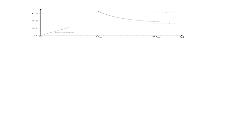
Figure 1: $(M,n)$ phase diagram for $d=5$ containing the uniform string branch and the non-uniform string branch of Wiseman. The black hole branch is sketched.

We thus see that all the known solutions corresponding to black holes or black strings can be mapped in our $(M,n)$ phase diagram, as done in the phase diagram of Figure 1.

4 Thermodynamics in the $(M,n)$ phase diagram

In this section we first derive a new Smarr formula for static and neutral black holes/strings on cylinders. We then show how one can use this to study the thermodynamics of branches of solutions in the $(M,n)$ phase diagram.

To derive the new Smarr formula, we begin by considering the Komar integral

$$I_{S}=-\frac{1}{16\pi G_{N}}\int_{S}dS_{\mu\nu}D^{\mu}k^{\nu}\ ,$$ (4.1)

where $S$ is a $d-1$ dimensional hypersurface in the $d+1$ dimensional cylinder space-time and $k$ is a killing vector for the metric. We can also write this integral as

$$I_{S}=-\frac{1}{16\pi G_{N}}\int_{S}\sqrt{-g}\frac{1}{(d-1)!}\epsilon_{\mu\nu\kappa^{1}\cdots\kappa^{d-1}}D^{\mu}k^{\nu}\,dx^{\kappa_{1}}\wedge\cdots\wedge dx^{\kappa_{d-1}}\ .$$ (4.2)

Consider now a static neutral solution on the cylinder with an event horizon. Consider furthermore a certain time $t=t_{0}$. Define $S_{h}$ to be the null-surface of the event horizon at $t=t_{0}$. We also choose a $d-1$ dimensional surface at $r=\infty$ for $t=t_{0}$, which we call $S_{\infty}$, so that essentially $S_{\infty}=S^{d-2}\times S^{1}$. By Gauss theorem we have

$$I_{S_{h}}-I_{S_{\infty}}=\frac{1}{16\pi G_{N}}\left(\int_{S_{\infty}}dS_{\mu\nu}D^{\mu}k^{\nu}-\int_{S_{h}}dS_{\mu\nu}D^{\mu}k^{\nu}\right)=\frac{1}{8\pi G_{N}}\int_{V}dS_{\mu}D_{\nu}D^{\mu}k^{\nu}\ ,$$ (4.3)

where $V$ is the $d$ dimensional volume between $S_{h}$ and $S_{\infty}$ so that $\partial V=S_{h}\cup S_{\infty}$. Since for a killing vector we have $D_{\nu}D^{\mu}k^{\nu}=R^{\mu}_{\ \nu}k^{\nu}$ and since $R_{\mu\nu}=0$ everywhere in $V$, as we are away from the black hole/string, it follows that $D_{\nu}D^{\mu}k^{\nu}=0$. Thus, we find that $I_{S_{h}}=I_{S_{\infty}}$.

Since we have a static solution we can choose $k$ to be the time-translation killing vector field, i.e. $k=\partial/\partial t$. On the event horizon $S_{h}$ we can choose a normal $n$ such that $k_{\mu}n^{\mu}=-1$. Then one can show that $dS_{\mu\nu}=(k_{\mu}n_{\nu}-k_{\nu}n_{\mu})dA$ where $dA$ is the area element on the event horizon (see [29]). Using this, we have [29]

$$I_{S_{h}}=-\frac{1}{8\pi G_{N}}\int_{S_{h}}dAk^{\nu}(D_{\nu}k^{\mu})n_{\mu}=-\frac{\kappa}{8\pi G_{N}}\int_{S_{h}}dAk^{\mu}n_{\mu}=\frac{\kappa A}{8\pi G_{N}}=TS\ ,$$ (4.4)

where we used that $k^{\nu}D_{\nu}k^{\mu}=\kappa\,k^{\mu}$. Here $\kappa$ is the surface gravity, $k_{\mu}n^{\mu}=-1$ and we used the thermodynamic identifications $\kappa=2\pi T$ and $A=4G_{N}S$. On the other hand, we have asymptotically

$$I_{S_{\infty}}=-\frac{1}{16\pi G_{N}}\int_{S_{\infty}}dS_{0r}\partial_{r}g_{00}=\frac{\Omega_{d-2}2\pi R_{T}}{16\pi G_{N}}(d-3)c_{t}=\frac{d-2-n}{d-1}M\ ,$$ (4.5)

where we first used that the non-zero components of $D^{\mu}k^{\nu}$ are $D^{0}k^{r}=-D^{r}k^{0}=\frac{1}{2}\partial_{r}g_{00}$ to leading order, and (2.18) in the last step.

In conclusion, we get from (4.4) and (4.5) that

$$TS=\frac{d-2-n}{d-1}M\ .$$ (4.6)

This is a new Smarr formula which holds for any static and neutral black hole/string on a cylinder. Indeed the Smarr formula (4.6) can be checked for all three known branches in the phase diagram. For uniform black strings ($n=1/(d-2)$) as well as for small black holes on the cylinder ($n=0$) it reduces to known Smarr relations. In Appendix C we show that the formula also holds to very high precision for the non-uniform black string branch using the numerical data of Wiseman.

Define now a branch to be a series of solutions corresponding to a curve in the $(M,n)$ diagram for which the first law of thermodynamics $\delta M=T\delta S$ is obeyed when moving between the solutions. Then if we consider a branch for which we know the precise curve in the $(M,n)$ phase diagram, we can find the thermodynamics on the branch. For simplicity we consider here the case where the curve is given by a function $n=n(M)$. Using now $\delta M=T\delta S$ and the Smarr formula (4.6) we get

$$\frac{\delta\log S}{\delta M}=\frac{1}{M}\frac{d-1}{d-2-n(M)}\ .$$ (4.7)

Thus, we see we only need to know the entropy in one point of the branch to find the complete function $S(M)$ for the branch. A similar statement applies to the temperature. In conclusion, knowing the exact curve of a branch in the $(M,n)$ phase diagram enables one to obtain the entire thermodynamics of that branch.

Another useful feature of depicting a branch in the $(M,n)$ phase diagram is that when two branches intersect we have the following Intersection Rule stating which branch has the highest entropy. The proof of the Intersection Rule is at the end of this section.

• Intersection Rule
  Consider two branches $\gamma_{1,2}$ in the $(M,n)$ phase diagram, parameterized by the functions $n_{1}(M)$ and $n_{2}(M)$. Let the range of masses be from $M^{\prime}$ to $M^{\prime\prime}$ ($M^{\prime}<M^{\prime\prime}$) and assume that $n_{1}(M)>n_{2}(M)$ for $M^{\prime}<M<M^{\prime\prime}$. Then

  $$\gamma_{1}\mbox{ intersect }\gamma_{2}\mbox{ at }M=M^{\prime}\ \Rightarrow\ S_{1}(M)>S_{2}(M)\mbox{ for }M>M^{\prime}\ ,$$ (4.8)

  and

  $$\gamma_{1}\mbox{ intersect }\gamma_{2}\mbox{ at }M=M^{\prime\prime}\ \Rightarrow\ S_{1}(M)<S_{2}(M)\mbox{ for }M<M^{\prime\prime}\ .$$ (4.9)

Thus, we see that for two intersecting branches we have the property that for masses below an intersection point the branch with the lower relative binding energy has the highest entropy, whereas for masses above an intersection point it is the branch with the higher relative binding energy that has the highest entropy. We have illustrated this in Figure 2.

Figure 2: Illustration of the Intersection Rule.

As a consequence of the Intersection Rule, we find that it is impossible for two branches which are described by well-defined functions $n=n(M)$ to intersect twice. If we write the two functions corresponding to the two branches as $n_{1}(M)$ and $n_{2}(M)$ and the two intersections as $M^{\prime}$ and $M^{\prime\prime}$, then the Intersection Rule gives a clear contradiction since we get from (4.8) that $S_{1}(M^{\prime\prime})>S_{2}(M^{\prime\prime})$ and from (4.9) that $S_{1}(M^{\prime})<S_{2}(M^{\prime})$ both of which contradict the fact that the two branches intersect in $M^{\prime}$ and $M^{\prime\prime}$.

We remind the reader of the physical reason why we are comparing the entropy of two branches at a given value of $M$, i.e. in the micro canonical ensemble. This is because, in order to address the stability of a particular branch, one would like to examine whether it is entropically favorable for the solution to move to another branch, characterized by a different value of the relative binding energy, by redistributing its mass.

The proof of above stated Intersection Rule goes as follows. Let $S_{i}(M)\equiv S(M,n_{i}(M))$, $i=1,2$ be the entropy on the two branches $\gamma_{1,2}$. If the two branches meet at $M=M_{\star}$ we can write the relation

$$\frac{S_{1}(M)}{S_{2}(M)}=1+\int_{M_{\star}}^{M}\delta\tilde{M}\frac{\delta}{\delta\tilde{M}}\left(\frac{S_{1}(\tilde{M})}{S_{2}(\tilde{M})}\right)\ .$$ (4.10)

Obviously $M_{\star}$ is either $M^{\prime}$ or $M^{\prime\prime}$. Consider now the differential

$$\frac{\delta}{\delta M}\left(\frac{S_{1}(M)}{S_{2}(M)}\right)=\frac{T_{2}S_{2}-T_{1}S_{1}}{T_{1}T_{2}S_{2}^{2}}=(n_{1}-n_{2})\frac{M}{(d-1)T_{1}T_{2}S_{2}^{2}}\ ,$$ (4.11)

where we used the first law of thermodynamics $\delta M_{i}=T_{i}\delta S_{i}$ for each of the branches in the first step and the Smarr formula (4.6) in the second step. Since we assume that $n_{1}(M)>n_{2}(M)$ for $M^{\prime}<M<M^{\prime\prime}$ we have

$$\frac{\delta}{\delta M}\left(\frac{S_{1}(M)}{S_{2}(M)}\right)>0\mbox{ for }M^{\prime}<M<M^{\prime\prime}\ .$$ (4.12)

Using (4.12) along with (4.10), we see that putting $M_{\star}=M^{\prime}$ gives (4.8) and putting $M_{\star}=M^{\prime\prime}$ gives (4.9), completing the proof.

5 Virtues of the $(M,n)$ diagram and comparison to the $(\lambda,M)$ diagram

So far in the literature, the phase diagram used to display the various phases of strings and black holes on cylinders has been what we call the $(\lambda,M)$ diagram. It is defined using the so-called non-uniformity parameter of [4]

$$\lambda=\frac{1}{2}\left(\frac{R_{\rm max}}{R_{\rm min}}-1\right)\ ,$$ (5.1)

where $R_{\rm max}$ and $R_{\rm min}$ are defined respectively as the maximal and the minimal radius of the $S^{d-2}$ sphere on the horizon. Note that $\lambda$ is invariant under coordinate transformations. In the following we discuss some important differences between the $(\lambda,M)$ and the $(M,n)$ phase diagrams.

An immediate physical point to notice is that $M$ and $n$ completely characterize the leading correction to the space-time at infinity. Thus, if an observer at infinity should draw diagrams of his/her findings, it would be natural to draw these in an $(M,n)$ phase diagram. In contrast, $\lambda$ can not be measured at infinity, since to know $\lambda$ one has to know the space-time all the way to the horizon.

Note also that the parameter $n$ always stays finite contrary to $\lambda$ which is infinite for the black hole branch since $R_{\rm min}=0$ on this branch. Moreover, we have already noted in Section 2 that $0\leq n\leq d-2$. However, we do not expect $n>1/(d-2)$ since it seems reasonable to assume that the uniform string branch, which has $n=1/(d-2)$, has the maximal possible relative binding energy. We therefore have the bound $0\leq n\leq\frac{1}{d-2}$. That $n$ is bounded makes it useful as a measure for “how far away” a given string solution is from a given black hole solution.

However, we should note that the $(\lambda,M)$ diagram has information that the $(M,n)$ diagram does not: The value of $\lambda$ explicitly states whether a solution is a uniform string, a non-uniform string or a black hole. On the other hand, as we described in Section 4, the $(M,n)$ phase diagram has several useful features. For example we have explained how one can read off the thermodynamics of a branch of solutions using the $(M,n)$ diagram. Moreover, it was explained that there are certain rules in the $(M,n)$ diagram restricting which branches are possible.

6 Discussion and conclusions

We have discussed in this paper a novel type of phase diagram for black holes and black strings on cylinders. The phase diagram involves, beyond the mass $M$, a new asymptotic quantity $n$, which is the relative binding energy in the circle direction. So far, three branches of solutions are known in the phase diagram: the uniform black string, the non-uniform string solutions numerically obtained by Wiseman [5] (see also [4]) and the small black hole branch. We have plotted these known branches in the new phase diagram.

We have derived a new Smarr formula, valid for black holes and strings on the cylinder, which involves the quantity $n$. This Smarr formula provides a powerful instrument as it enables one to obtain the entire thermodynamics, once the solution $n(M)$ in the phase diagram is known. Moreover, when combined with the first law of thermodynamics, the Smarr formula also implies an Intersection Rule, which easily determines the branch of highest entropy for intersecting branches in the phase diagram. Although we have focussed in this paper on neutral black holes/strings, this part of the development is easily generalized to the non-extremal and near-extremal case as well as the inclusion of angular momenta. For example, in the non-extremal case, the Smarr formula is simply obtained by $M\rightarrow M-\mu Q$ in (4.6).

We also remark that the formalism introduced in this paper seems well-suited for the important study of the phase structure of black $p$-branes in spaces with more than one compact direction. The simplest generalization one can think of would be to study black holes, strings and membranes on the torus $\mathbb{R}^{d-2}\times T^{2}$. Following our development, one would need in that case, beyond the mass $M$, three additional asymptotic quantities corresponding to the stress in the torus direction.

We have pointed out some of the virtues of the $(M,n)$ phase diagram and compared to the $(\lambda,M)$ diagram, so far used in the literature. In a forthcoming work [30] we will use the formalism introduced in this paper to obtain various new insights into the phase structure for black holes and strings on cylinders.

Finally, we comment on the issue of uniqueness of black hole/string solutions on a cylinder. We obtained in Section 2 the gauge invariant quantities that determine the leading order metric in the presence of a static and neutral (spherical symmetric) mass distribution on the cylinder. Beyond the mass $M$ and the relative binding energy $n$, these were shown to also involve the higher Fourier modes $\varrho_{k\geq 1}$ of the mass distribution. For black holes/strings on cylinders this implies the possibility of having several solutions for a given point in the $(M,n)$ phase diagram, distinguished by the $\varrho_{k}$.

For neutral black holes in four space time dimensions it is well-known that the solution is uniquely characterized given the mass. It would naturally be very interesting to examine whether similar uniqueness theorems hold for black holes/strings on cylinders. For example, it may be that the Fourier modes $\varrho_{k}$ are determined in terms of $M$ and $n$. It is thus conceivable that the following uniqueness hypothesis is valid:

• Consider solutions of the Einstein equations on a cylinder $\mathbb{R}^{d-1}\times S^{1}$. For a given mass $M$ and relative binding energy $n$ there exists at most one neutral and static solution of the Einstein equations with an event horizon.

A less strong version of the above hypothesis would be that also the choice of horizon topology ($S^{d-2}\times S^{1}$ or $S^{d-1}$) needs to be specified in order to obtain a unique solution.

Appendix A Green function on a cylinder

We consider the cylinder $\mathbb{R}^{d-1}\times S^{1}$ with metric

$$ds^{2}=dz^{2}+dr^{2}+r^{2}d\Omega_{d-2}^{2}\ .$$ (A.1)

where $z$ is periodic with period $2\pi R_{T}$. Here the $S^{d-2}$ sphere is parameterized by the angles $\theta_{1},...,\theta_{d-2}$ and it has the metric

$$d\Omega_{d-2}^{2}=\sum_{a,b=1}^{d-2}\gamma_{ab}\,d\theta_{a}d\theta_{b}\ .$$ (A.2)

Define $\gamma=\sqrt{\det(\gamma_{ab})}$. Define furthermore the notation $\Theta=(\theta_{1},...\theta_{d-2})$.

We define then the Green function on $\mathbb{R}^{d-1}\times S^{1}$ as

$$\nabla_{z,r,\Theta}^{2}G(z-z^{\prime},r-r^{\prime},\Theta-\Theta^{\prime})=-\frac{\Omega_{d-2}}{r^{d-2}\gamma}\delta(z-z^{\prime})\delta(r-r^{\prime})\delta(\Theta-\Theta^{\prime})\ .$$ (A.3)

In the following we derive a useful expansion of the Green function on the cylinder which is used in Section 2.

We first introduce the spherical harmonics $Y_{l}(\Theta)$ which are eigenfunctions

$$\frac{1}{\gamma}\sum_{a=1}^{d-2}\partial_{\theta_{a}}\left[\gamma\gamma^{ab}\partial_{\theta_{b}}Y_{l}(\theta_{1},...,\theta_{d-2})\right]=-h_{l}Y_{l}(\theta_{1},...,\theta_{d-2})\ ,$$ (A.4)

that satisfy the completeness relation

$$\sum_{l}Y^{*}_{l}(\Theta^{\prime})Y_{l}(\Theta)=\frac{1}{\gamma}\delta(\Theta-\Theta^{\prime})\ .$$ (A.5)

We can now expand any function on $S^{d-2}$ as $f(\Theta)=\sum_{l}a_{l}Y_{l}(\Theta)$. We can furthermore expand the delta function for $z$ as

$$\delta(z-z^{\prime})=\frac{1}{2\pi R_{T}}\sum_{k\in\mathbb{Z}}e^{ik(z-z^{\prime})/R_{T}}=\frac{1}{2\pi R_{T}}\left[1+2\sum_{k=1}^{\infty}\cos\!\left(\frac{k(z-z^{\prime})}{R_{T}}\right)\right]\ .$$ (A.6)

The Green function can then be expanded as

$$G(z-z^{\prime},r-r^{\prime},\Theta-\Theta^{\prime})=\frac{1}{2\pi R_{T}}\sum_{l}Y^{*}_{l}(\Theta^{\prime})Y_{l}(\Theta)\sum_{k\in\mathbb{Z}}M^{(k)}_{l}(r,r^{\prime})e^{ik(z-z^{\prime})/R_{T}}\ .$$ (A.7)

Using this the Green function equation (A.3) then becomes equivalent to

$$\left(\partial_{r}^{2}+\frac{d-2}{r}\partial_{r}\right)M^{(k)}_{l}(r,r^{\prime})-\left(\frac{k^{2}}{R_{T}^{2}}+\frac{h_{l}}{r^{2}}\right)M^{(k)}_{l}(r,r^{\prime})=-\frac{\Omega_{d-2}}{r^{d-2}}\delta(r-r^{\prime})\ .$$ (A.8)

In order to solve this equation, we notice that the modified Bessel functions of the second kind $K_{\nu}(x)$ and $I_{\nu}(x)$ are solutions to the equation

$$f^{\prime\prime}+\frac{1}{x}f^{\prime}-\left(1+\frac{\nu^{2}}{x^{2}}\right)f=0\ .$$ (A.9)

Notice then that if we define $g$ as

$$g(x)=x^{-\frac{d-3}{2}}f(kx)\ ,$$ (A.10)

then $g$ is a solution to the equation

$$g^{\prime\prime}+\frac{d-2}{x}g^{\prime}-\left[k^{2}+\left(\nu^{2}-\frac{1}{4}(d-3)^{2}\right)\right]g=0\ .$$ (A.11)

So, using

$$\nu_{l}=\sqrt{\frac{1}{4}(d-3)^{2}+h_{l}}\ ,$$ (A.12)

we see that $g(r/R_{T})$ is a solution of (A.8) when $r\neq r^{\prime}$. Define now the two independent solutions of the differential equation (A.11) by

$$\psi_{1}^{(k)}(\nu,x)=k^{-\nu}x^{-\frac{d-3}{2}}I_{\nu}(kx)\ ,\ \ \psi_{2}^{(k)}(\nu,x)=k^{\nu}x^{-\frac{d-3}{2}}K_{\nu}(kx)\ ,$$ (A.13)

satisfying

$$\psi_{1}^{(k)}(\nu,x)\simeq\frac{1}{2^{\nu}\Gamma(\nu+1)}x^{\nu-\frac{d-3}{2}}\ ,\ \ \psi_{2}^{(k)}(\nu,x)\simeq 2^{\nu-1}\Gamma(\nu)x^{-\nu-\frac{d-3}{2}}\ ,\ \ x\ll 1$$ (A.14)

$$\psi_{1}^{(k)}\frac{d}{dx}\psi_{2}^{(k)}-\psi_{2}^{(k)}\frac{d}{dx}\psi_{1}^{(k)}=-\frac{1}{x^{d-2}}\ .$$ (A.15)

Then we can write the solution of (A.8) as

$$M^{(k)}_{l}(r,r^{\prime})=\frac{\Omega_{d-2}}{R_{T}^{d-3}}\,\psi_{1}^{(k)}\!\left(\nu_{l},\frac{r_{<}}{R_{T}}\right)\psi_{2}^{(k)}\!\left(\nu_{l},\frac{r_{>}}{R_{T}}\right)\ ,$$ (A.16)

with

$$r_{<}=\left\{\begin{array}[]{ll}r\ ,&\ r<r^{\prime}\\ r^{\prime}\ ,&\ r>r^{\prime}\end{array}\right.\ ,\ \ r_{>}=\left\{\begin{array}[]{ll}r^{\prime}\ ,&\ r<r^{\prime}\\ r\ ,&\ r>r^{\prime}\end{array}\right.\ \ .$$ (A.17)

Appendix B Critical masses for the Gregory-Laflamme instability

For completeness we list in this appendix the Gregory-Laflamme masses for uniform black strings on a cylinder $\mathbb{R}^{d-1}\times S^{1}$ with $d=4,...,9$. The data has been taken from [1] (the published version) by reading off $\mu$ from their Fig. 1. The values of $\mu$ that we read off are $0.44,0.62,0.80,0.93,1.04,1.15$ for $d=4,...,9$. One can then see in [1, 2] that the critical horizon radius is given by $r_{0}/R_{T}=2\mu$, where $r_{0}$ is the horizon radius of the uniform black string solution (3.1) and $R_{T}$ is the radius of the cylinder. Using that

$$M=\frac{\Omega_{d-2}2\pi R_{T}}{16\pi G_{N}}(d-2)r_{0}^{d-3}\ ,$$ (B.1)

we can compute the critical masses. In Table 1 we have listed the horizon radii and the masses for $d=4,...,9$. We have used the notation that the circumference of the cylinder is $L=2\pi R_{T}$.

$d$	$4$	$5$	$6$	$7$	$8$	$9$
$r_{0}/L$	$0.14$	$0.20$	$0.25$	$0.30$	$0.33$	$0.37$
$16\pi G_{N}M_{\rm GL}/L^{d-2}$	$3.52$	$2.31$	$1.74$	$1.19$	$0.79$	$0.55$

Table 1: Critical horizon radii and masses for the Gregory-Laflamme instability.

Appendix C Details on Wiseman’s non-uniform black string data

In this appendix we provide the reader with details of how the plot of Wiseman’s non-uniform black string branch in Figure 1 was made. Wiseman’s non-uniform black string solutions (with $d=5$) were obtained in [5] by numerically solving Einstein’s equations for the conformal ansatz

$$ds_{6}^{2}=-\frac{r^{2}}{m+r^{2}}e^{2A}dt^{2}+e^{2B}(dr^{2}+dz^{2})+e^{2C}(m+r^{2})d\Omega_{3}^{2}\ .$$ (C.1)

Here, $A,B,C$ are functions of $(r,z)$, with asymptotic forms

$$A\simeq\frac{a_{2}}{r^{2}}\ ,\ \ B\simeq\frac{b_{2}}{r^{2}}\ ,\ \ C\simeq\frac{c_{1}}{r}+\frac{c_{2}}{r^{2}}\ .$$ (C.2)

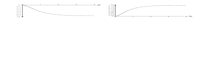
Figure 3: Plot of $a_{2}$ and $b_{2}$ versus $\lambda$ using the data of [5].

The data found in [5] consist of 25 points, each corresponding to a non-uniform black string solution. Each of the 25 points is then specified by six numbers: $\lambda$, $a_{2}$, $b_{2}$, $T_{\rm w}$, $S_{\rm w}$, and $M_{\rm w}$. $\lambda$ is defined in (5.1), $T_{\rm w}$, $S_{\rm w}$ and $M_{\rm w}$ are the temperature, entropy and mass that was computed in [5], and $a_{2}$ and $b_{2}$ are defined in (C.2). These data was generously made available to us by Toby Wiseman.

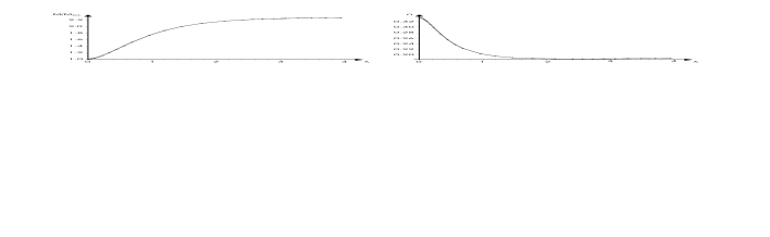
Figure 4: Plot of $M$ and $n$ versus $\lambda$. $M$ and $n$ are computed from the $a_{2}$ and $b_{2}$ data. The crosses mark the actual data-points.

Figure 5: Plot of $M$ versus $n$ as computed from the $a_{2}$ and $b_{2}$ data. The crosses mark the actual data-points.

The only data necessary to make the phase diagram in Figure 1 are $a_{2}$ and $b_{2}$ for the 25 points. We have plotted $a_{2}$ and $b_{2}$ versus $\lambda$ in Figure 3. We refer the reader to [5] for plots of $T_{\rm w}$, $S_{\rm w}$ and $M_{\rm w}$ versus lambda. By comparing (2.17) and (C.1)-(C.2) we see that $a_{2}$ and $b_{2}$ are related to $c_{t}$ and $c_{z}$ as

$$c_{t}=1-2a_{2}\ ,\ \ c_{z}=2b_{2}\ ,$$ (C.3)

where we note that $m=1$ in (C.1). We can then use this in (2.18) (with $d=5$) to determine the mass $M$ and relative binding energy $n$ for each data point according to

$$\frac{M}{M_{\rm GL}}=c_{t}-\frac{c_{z}}{3}\ ,\ \ n=\frac{c_{t}-3c_{z}}{3c_{t}-c_{z}}\ .$$ (C.4)

In Figure 4 we have plotted $M$ and $n$ versus $\lambda$. Moreover, in Figure 5 we have plotted $M$ versus $n$.

We now check that the first law of thermodynamics $\delta M=T\delta S$ is obeyed for the above computed $M$. In left graph of Figure 6 we have depicted $\delta M/\delta\lambda$ and $T\delta S/\delta\lambda$ versus $\lambda$. We note that they agree to a high precision. The third curve in Figure 6 is $\delta M_{w}/\delta\lambda$ where $M_{w}$ is the mass that Wiseman computed in the original version of [5]. We see that the systematic error that Wiseman noted in the original version of [5] in fact is due to an erroneous computation of the mass, and not an inaccuracy of the solutions that were found (see also comment in new version of [5]).

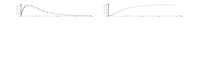
Figure 6: On the left plot we have checked the first law of thermodynamics for Wiseman’s branch of solutions. Here the solid curve shows $T\frac{\delta S}{\delta\lambda}$, the crosses show $\frac{\delta M}{\delta\lambda}$ and the diamonds show $\frac{\delta M_{w}}{\delta\lambda}$, all in units of $M_{GL}$. On the right plot we have checked Smarr’s formula (4.6). Here the solid curve show $TS$ while the crosses show $\frac{3-n}{4}M$, both in units of $T_{\rm GL}S_{\rm GL}=\frac{2}{3}M_{\rm GL}$.

In the right graph of Figure 6 we have instead plotted $TS$ (computed from $T_{w}$ and $S_{w}$) and $\frac{3-n}{4}M$ versus $\lambda$. This is a check of Smarr’s formula (4.6). We see that Smarr’s formula is correct to a very high precision.

References

- [1] R. Gregory and R. Laflamme, “Black strings and p-branes are unstable,” Phys. Rev. Lett. 70 (1993) 2837–2840, hep-th/9301052.
- [2] R. Gregory and R. Laflamme, “The instability of charged black strings and p-branes,” Nucl. Phys. B428 (1994) 399–434, hep-th/9404071.
- [3] G. T. Horowitz and K. Maeda, “Fate of the black string instability,” Phys. Rev. Lett. 87 (2001) 131301, hep-th/0105111.
- [4] S. S. Gubser, “On non-uniform black branes,” Class. Quant. Grav. 19 (2002) 4825–4844, hep-th/0110193.
- [5] T. Wiseman, “Static axisymmetric vacuum solutions and non-uniform black strings,” Class. Quant. Grav. 20 (2003) 1137–1176, hep-th/0209051.
- [6] R. Gregory and R. Laflamme, “Hypercylindrical black holes,” Phys. Rev. D37 (1988) 305.
- [7] M. W. Choptuik et al., “Towards the final fate of an unstable black string,” Phys. Rev. D68 (2003) 044001, gr-qc/0304085.
- [8] T. Harmark and N. A. Obers, “Black holes on cylinders,” JHEP 05 (2002) 032, hep-th/0204047.
- [9] G. T. Horowitz, “Playing with black strings,” hep-th/0205069.
- [10] B. Kol, “Topology change in general relativity and the black-hole black-string transition,” hep-th/0206220.
- [11] T. Wiseman, “From black strings to black holes,” Class. Quant. Grav. 20 (2003) 1177–1186, hep-th/0211028.
- [12] T. Harmark and N. A. Obers, “Black holes and black strings on cylinders,” Fortsch. Phys. 51 (2003) 793–798, hep-th/0301020.
- [13] B. Kol and T. Wiseman, “Evidence that highly non-uniform black strings have a conical waist,” Class. Quant. Grav. 20 (2003) 3493–3504, hep-th/0304070.
- [14] R. Casadio and B. Harms, “Black hole evaporation and large extra dimensions,” Phys. Lett. B487 (2000) 209–214, hep-th/0004004.
- [15] R. Casadio and B. Harms, “Black hole evaporation and compact extra dimensions,” Phys. Rev. D64 (2001) 024016, hep-th/0101154.
- [16] G. T. Horowitz and K. Maeda, “Inhomogeneous near-extremal black branes,” Phys. Rev. D65 (2002) 104028, hep-th/0201241.
- [17] P.-J. De Smet, “Black holes on cylinders are not algebraically special,” Class. Quant. Grav. 19 (2002) 4877–4896, hep-th/0206106.
- [18] B. Kol, “Speculative generalization of black hole uniqueness to higher dimensions,” hep-th/0208056.
- [19] E. Sorkin and T. Piran, “Initial data for black holes and black strings in 5d,” Phys. Rev. Lett. 90 (2003) 171301, hep-th/0211210.
- [20] A. V. Frolov and V. P. Frolov, “Black holes in a compactified spacetime,” Phys. Rev. D67 (2003) 124025, hep-th/0302085.
- [21] R. Emparan and R. C. Myers, “Instability of ultra-spinning black holes,” JHEP 09 (2003) 025, hep-th/0308056.
- [22] B. Kol, E. Sorkin, and T. Piran, “Caged black holes: Black holes in compactified spacetimes I – theory,” hep-th/0309190.
- [23] J. Traschen and D. Fox, “Tension perturbations of black brane spacetimes,” gr-qc/0103106.
- [24] P. K. Townsend and M. Zamaklar, “The first law of black brane mechanics,” Class. Quant. Grav. 18 (2001) 5269–5286, hep-th/0107228.
- [25] J. Traschen, “A positivity theorem for gravitational tension in brane spacetimes,” hep-th/0308173.
- [26] T. Shiromizu, D. Ida, and S. Tomizawa, “Kinematical bound in asymptotically translationally invariant spacetimes,” gr-qc/0309061.
- [27] E. Witten, “A simple proof of the positive energy theorem,” Commun. Math. Phys. 80 (1981) 381.
- [28] G. W. Gibbons, S. W. Hawking, G. T. Horowitz, and M. J. Perry, “Positive mass theorems for black holes,” Commun. Math. Phys. 88 (1983) 295.
- [29] P. K. Townsend, “Black holes,” gr-qc/9707012.
- [30] T. Harmark and N. A. Obers, “Phase structure of black holes and strings on cylinders,” hep-th/0309230.
- [31] R. Emparan and H. S. Reall, “A rotating black ring in five dimensions,” Phys. Rev. Lett. 88 (2002) 101101, hep-th/0110260.