Extended $QCD_{2}$ from dimensional projection of $QCD_{4}$

Abstract:

We study an extended QCD model in $(1+1)$ dimensions obtained from QCD in $4D$ by compactifying two spatial dimensions and projecting onto the zero-mode subspace. We work out this model in the large $N_{c}$ limit and using light cone gauge but keeping the equal-time quantization. This system is found to induce a dynamical mass for transverse gluons – adjoint scalars in $QCD_{2}$, and to undergo a chiral symmetry breaking with the full quark propagators yielding non-tachyonic, dynamical quark masses, even in the chiral limit. We study quark-antiquark bound states which can be classified in this model by their properties under Lorentz transformations inherited from $4D$. The scalar and pseudoscalar sectors of the theory are examined and in the chiral limit a massless ground state for pseudoscalars is revealed with a wave function generalizing the so called ’t Hooft pion solution.

1 Introduction

It is fairly well accepted that Quantum Chromodynamics (QCD) is a correct theory of strong interactions giving a good description of the high energy scattering of hadrons. However our ability to develop its predictions at low energies, the non-perturbative regime of QCD, is not as good. The latter problem can be handled more easily if we consider a lower dimensional space. In this way, QCD in two dimensions, $QCD_{2}$, first studied by ’t Hooft in the large $N_{c}$ limit [1, 2], has proved to be a very interesting laboratory for checking non-perturbative aspects of QCD.

This model has been a subject of extensive investigation, covering the study of quark confinement, hadron form factors, deep-inelastic [3, 4] and hadron-hadron scattering [5], the role of instantons and solitons [6, 7], multi-flavor states [8], quark condensation [9] and heavy quark physics [10]. The bosonization of $QCD_{2}$ was used as a tool for the description of meson and baryon spectra [11, 12, 13] and of chiral symmetry breaking [12, 14].

The remarkable feature of this model is that it exhibits quark confinement with an approximately linear Regge trajectory for the masses of $q{\bar{q}}$ bound states [2]. As well $QCD_{2}$ in the large $N_{c}$ limit has an interpretation in terms of string variables [15] sharing thereby important properties that we expect to find for real QCD in four dimensions.

However $QCD_{2}$ is too simple to describe certain realistic aspect of the higher dimensional theory. For instance, there are no physical gluons in two dimensions and both angular momentum and spin are absent in a $2D$ theory. Moreover in $QCD_{2}$ there is a problem of tachyonic properties of ’t Hooft quarks [2] and a realistic chiral symmetry breaking is absent which manifests itself in the decoupling of massless pions [16]. Thus one needs more information from extra dimensions in order to have a more realistic picture of QCD by using a $2D$ model. For instance, the inclusion of boson matter in the adjoint gauge group representation [17, 18] may provide an information of transverse degrees of freedom, characteristic of a gauge theory in higher dimensions, and give a more adequate picture of strong interaction.

In this paper we study a QCD reduced model in $(1+1)$ dimensions which can be formally obtained from QCD in $4D$ by means of a classical dimensional reduction from $4D$ to $2D$ and neglecting heavy K-K (Kaluza-Klein) states. Thus only zero-modes in the harmonic expansion in compactified dimensions are retained. As a consequence, we obtain a two dimensional model with some resemblances of the real theory in higher dimension, that is, in a natural way adding boson matter in the adjoint representation to $QCD_{2}$. The latter fields being scalars in $2D$ reproduce transverse gluon effects. Furthermore this model has a richer spinor structure than just $QCD_{2}$ giving a better resolution of scalar and vector states which can be classified by their properties inherited from $4D$ Lorentz transformations. The model is analyzed in the light cone gauge and using large $N_{c}$ limit. The contributions of the extra dimensions are controlled by the radiatively induced masses of the scalar gluons as they carry a piece of information of transverse degrees of freedom. We consider their masses as large parameters in our approximations yet being much less than the first massive K-K excitation. However this model is treated on its own ground without any further comparison with possible contributions of heavier K-K boson states. As well we do not pay any attention to the mass generation via Hosotani mechanism [19] as it has no significance in the planar limit of two-dimensional QCD models under consideration, just being saturated by fermion loops sub-leading in the $1/N_{c}$ expansion.

This model might give more insights into the chiral symmetry breaking regime of $QCD_{4}$. Namely, we are going to show that the inclusion of solely lightest K-K boson modes catalyze the generation of quark dynamical mass and allows us to overcome the problem of tachyonic quarks present in $QCD_{2}$.

The paper is written as follows, in Sect. 2 we make a formal design of the $2D$ reduced model from QCD in $4D$ by using Kaluza-Klein compactification and further projection onto zero-mode subspace. First we work with the gluon part of $QCD_{4}$ which is mapped into a $2D$ $SU\!(N)$ gauge field and two scalar fields in the adjoint representation of the reduced gauge model. In principle, these scalars are massless but we recover an infrared generation of masses for these scalar gluons. Next we examine the fermion part of $QCD_{4}$ and after compactifying and projecting we obtain two spinors minimally coupled to the $2D$ gauge field and interacting with the scalar gluons. The full propagator for these fermions is calculated in the large $N_{c}$ limit by using the Schwinger-Dyson equation and a non-perturbative solution for the self-energy is found that gives a real net quark mass, even in the chiral limit [20]. In Sect. 3 we study bound states of quark and antiquark by using the Bethe-Salpeter equation in the large $N_{c}$ and the ladder approximations. $q{\bar{q}}$ states of the model are identified in terms of their custodial symmetries from $4D$ Lorentz group. We focus our attention on the scalar and pseudoscalar sectors of the theory and in Sect. 4 the low mass spectrum of the scalar and pseudoscalar sector is examined. In the chiral limit, a massless ground state is revealed which is interpreted as the pion of the model, a projection of the real Goldstone boson in $4D$ to $2D$ treated in the large-$N_{c}$ limit. We summarize our points and give conclusions in Sect. 5.

2 Compactification of $QCD_{4}$ to the Reduced Model

2.1 The Gluon Part

We start with the $QCD_{4}$ action for gluons in $(3+1)$ dimensions:

$$S_{QCD}=-\int d^{4}x\frac{1}{2{\tilde{g}}^{2}}tr(G_{\mu\nu}^{2})\,,$$ (1)

where:

$$G_{\mu\,\nu}=\partial_{\mu}G_{\nu}-\partial_{\nu}G_{\mu}-i\left[G_{\mu},G_{\nu}\right],$$ (2)

with $G_{\mu}=G^{a}_{\mu}\,\lambda_{a}$. Generators $\lambda_{a}$ and structure constants $f_{abc}$ satisfy:

$$tr(\lambda_{a}\lambda_{b})=\frac{1}{2}\delta_{ab}\,, \left[\lambda_{a},\lambda_{b}\right]=if_{abc}\lambda_{c}\,.$$ (3)

Now we proceed to make a dimensional reduction of QCD, at the classical level, from $4D$ to $2D$. For this we consider the coordinates $x_{2,3}$ being compactified in a 2-Torus, respectively the fields being periodic on the intervals ($0\leq x_{2,3}\leq L=2\pi R$). Next we assume $L$ to be small enough in order to get an effective model in $1+1$ dimensions.

Following this scheme we expand the fields in Fourier modes on the compactified dimensions:

$$G_{\mu}(x_{0},x_{1},x_{2},x_{3})=\sum_{n,m=-\infty}^{\infty}exp\left\{\frac{2\pi i}{L}[nx_{2}+mx_{3}]\right\}G^{n,m}_{\mu}(x_{0},x_{1}).$$ (4)

By integrating heavy K-K modes Eq. (4) with $n,m\not=0$ in the QCD generating functional we obtain the low-energy effective action for zero-modes which can be efficiently prepared along the Wilson construction with the help of a cutoff $\Lambda$. Accordingly, let us adopt the low-energy limit $|p_{0,1}|\ll m_{KK}^{n,m}=\frac{2\pi}{L}\sqrt{n^{2}+m^{2}};\quad n,m\not=0$. Hence if we choose a $2D$ cutoff $\Lambda\simeq\frac{1}{R}=\frac{2\pi}{L}$ larger than the typical momenta $p_{0,1}$, we are led to analyze the zero Fourier modes only. Thus all relevant fields on the uncompactified $1+1$ space-time consist of zero modes.

To make contact with ’t Hooft solution, we introduce light-cone coordinates in the uncompactified space-time $x_{\pm}=\frac{1}{\sqrt{2}}(x_{0}\pm x_{1})$, then we obtain $A_{\pm}=\frac{1}{\sqrt{2}}(G_{0}\pm G_{1})$ and two scalar fields defined as $\phi_{1,2}=G_{2,3}$.

By keeping only the zero K-K modes , we get the following effective action:

$$S=\int d^{2}x\frac{L^{2}}{{\tilde{g}}^{2}}\,tr\!\left[(\partial_{-}A_{+}-\partial_{+}A_{-}-i[A_{-},A_{+}])^{2}+2(\partial_{-}\phi_{1}-i[A_{-},\phi_{1}])(\partial_{+}\phi_{1}-i[A_{+},\phi_{1}])+\right.$$

$$\left.2(\partial_{-}\phi_{2}-i[A_{-},\phi_{2}])(\partial_{+}\phi_{2}-i[A_{+},\phi_{2}])+[\phi_{1},\phi_{2}]^{2}\right].$$ (5)

Following the t’Hooft scheme we choose the light-cone gauge $A_{-}=0$. Then the action is transformed to:

$$S=\int d^{2}x\frac{L^{2}}{{\tilde{g}}^{2}}\,tr\!\left[(\partial_{-}A_{+})^{2}-2iA_{+}\left([\phi_{1},\partial_{-}\phi_{1}]+[\phi_{2},\partial_{-}\phi_{2}]\right)\right.$$

$$\left.+2(\partial_{-}\phi_{1}\partial_{+}\phi_{1}+\partial_{-}\phi_{2}\partial_{+}\phi_{2})+[\phi_{1},\phi_{2}]^{2}\right].$$ (6)

This action is quadratic in $A_{+}$. To analyze the mass spectra for fields $\phi_{1,2}$, we integrate over $A_{+}$:

$$S_{\phi}=\int d^{2}x\,\,\frac{L^{2}}{{\tilde{g}}^{2}}tr\{2\partial_{-}\phi_{k}\partial_{+}\phi_{k}+[\phi_{1},\phi_{2}]^{2}$$

$$-\int d^{2}y\left([\phi_{1},\partial_{-}\phi_{1}]+[\phi_{2},\partial_{-}\phi_{2}]\right)\langle x|P.V.\frac{1}{\partial_{-}^{2}}|y\rangle(\phi_{k}\partial_{-}\phi_{k})\}.$$ (7)

We expect the infrared mass generation for the two-dimensional scalar gluons $\phi_{1,2}$ [21]. Let us calculate it to the leading order of perturbation theory. Applying the Background Field Method we split $\phi=\frac{{\tilde{g}}}{L}(\phi_{c}+\eta)$, with $\phi_{c}$ being a constant background. Then the one-loop contribution is given by:

$$S^{(2)}=\int d^{2}x\,\mbox{\rm tr}\Bigl{\{}2\partial_{-}\eta_{k}\partial_{+}\eta_{k}+\frac{{\tilde{g}}^{2}}{L^{2}}([\phi_{2c},\eta_{1}]^{2}+[\phi_{1c},\eta_{2}]^{2})$$ (8)

$$-\frac{{\tilde{g}}^{2}}{L^{2}}\int d^{2}y\,\partial_{-}([\phi_{kc},\eta_{k}(x)])\langle x|\frac{1}{\partial_{-}^{2}}|y\rangle\partial_{-}([\phi_{kc},\eta_{k}(y)])$$

$$+2\frac{{\tilde{g}}^{2}}{L^{2}}([\eta_{1},\eta_{2}][\phi_{1c},\phi_{2c}]+[\phi_{1c},\eta_{2}][\eta_{1},\phi_{2c}])\Bigl{\}}.$$

The masses can be calculated from the quadratic part of the effective potential, after integration by parts:

$$S^{(2)}=\int d^{2}x\,\mbox{\rm tr}\Bigl{\{}2\partial_{-}\eta_{1}\partial_{+}\eta_{1}+2\partial_{-}\eta_{2}\partial_{+}\eta_{2}$$

$$+\frac{{\tilde{g}}^{2}}{L^{2}}([\phi_{1c},\eta_{1}]^{2}+[\phi_{2c},\eta_{1}]^{2}+[\phi_{1c},\eta_{2}]^{2}+[\phi_{2c},\eta_{2}]^{2})\Bigr{\}},$$ (9)

They receive equal pieces from the two-dimensional gluon exchange and the tadpole.

To estimate the masses of scalar gluons $\phi$ we use the Schwinger-Dyson equations as self-consistency conditions:

$$M^{2}=\frac{2N_{c}{\tilde{g}}^{2}}{L^{2}}\int^{\Lambda}\!\!\frac{d^{2}p}{(2\pi)^{2}}\,\frac{1}{p^{2}+M^{2}}\,=\frac{N_{c}{\tilde{g}}^{2}\,\Lambda^{2}}{8\pi^{3}}\,\,\log\frac{\Lambda^{2}+M^{2}}{M^{2}}\,,$$ (10)

thus $M^{2}$ brings an infrared cutoff as expected. We notice that the gluon mass remains finite in the large-$N_{c}$ limit if the QCD coupling constant decreases as $1/N_{c}$ in line with the perturbative law of $4D$ QCD. Respectively such a mass would dominate over the mass induced by the Hosotani mechanism as the latter one is sub-leading in $1/N_{c}$ if being provided by fermions in the fundamental representation [19].

We adopt the approximation $M\ll\Lambda\simeq 1/R$ to protect the low-energy sector of the model and consider the momenta $|p_{0,1}|\sim M$. Thereby we retain only leading terms in the expansion in $\frac{p^{2}}{\Lambda^{2}}$ and $\frac{M^{2}}{\Lambda^{2}}$, and also neglect the effects of the heavy K-K modes in the low-energy Wilson action.

Now we proceed to the evaluation of the model (5) as a generalization of the ’t Hooft $QCD_{2}$ and take a bounded value of $M$. Then the low-energy approximation corresponds to the small coupling constant:

$${\tilde{g}}^{2}\sim\frac{M^{2}}{N_{c}\Lambda^{2}}\frac{1}{\log\frac{\Lambda^{2}}{M^{2}}}\leq 1,$$ (11)

in accordance to Eq. (10). Thus the relevant coupling constant for the model (5) is:

$$g^{2}=\frac{N_{c}\,{\tilde{g}}^{2}}{L^{2}}=\frac{N_{c}\,{\tilde{g}}^{2}\,\Lambda^{2}}{4\pi^{2}}\sim\frac{M^{2}}{log\frac{\Lambda^{2}}{M^{2}}}.$$ (12)

This dimensional constant governs the meson mass spectrum of the ’t Hooft $QCD_{2}$ [1] and can be associated to a particular meson mass, i.e. be fixed. Then the gluon mass is slowly growing with the increasing cutoff $\Lambda$ and and the ”heavy-scalar” expansion parameter is:

$$A=\frac{g^{2}}{2\pi\,M^{2}}=\frac{1}{log\frac{\Lambda^{2}}{M^{2}}}.$$ (13)

We observe that the limit $M\ll\Lambda$ supports consistently both the fast decoupling of the heavy K-K modes and moderate decoupling of scalar gluons, the latter giving an effective four-fermion interaction different from [23]. Nevertheless we prefer to keep first the gluon mass finite and further on derive the expansion in parameter $A$ gradually from the Bethe-Salpeter equation because for small $A$ one recovers non-analytical infra-red effects for the ground state wave function.

2.2 Introducing fermions

Now let us make the K-K reduction of the quark part of $QCD_{4}$ at the classical level. The original Lagrangian reads,

$$S=\int\!d^{4}x{\bar{\Psi}}\,(i\gamma^{\mu}\,D_{\mu}-m)\,\Psi\,,$$ (14)

where the covariant derivative is defined conventionally: $D_{\mu}=\partial_{\mu}-i\,G_{\mu}$. The following representation of $\gamma$ matrices is employed:

$$\gamma_{0}=\left(\begin{array}[]{cc}\sigma_{1}&0\\ 0&\sigma_{1}\end{array}\right)\!,\gamma_{1}=\left(\begin{array}[]{cc}i\sigma_{2}&0\\ 0&i\sigma_{2}\end{array}\right)\!,\gamma_{2}=\left(\begin{array}[]{cc}0&i\sigma_{3}\\ i\sigma_{3}&0\end{array}\right)\!,\gamma_{3}=\left(\begin{array}[]{cc}i\sigma_{3}&0\\ 0&-i\sigma_{3}\end{array}\right)\!,\gamma_{5}=\left(\begin{array}[]{cc}0&-i\sigma_{3}\\ i\sigma_{3}&0\end{array}\right)\!,$$ (25)

suitable for the purposes of K-K reduction. Then the bispinor is decomposed into two-dimensional ones, $\Psi=\left(\begin{array}[]{c}\psi_{a}\\ \psi_{b}\end{array}\right)$ with the help of the projectors, $P_{a,b}=\frac{1}{2}(1\pm\gamma_{2}\,\gamma_{5})$.

Now we compactify on the torus and expand the fermion fields in Fourier modes of the compactified dimensions $x_{2,3}$:

$$\Psi(x_{0},x_{1},x_{2},x_{3})=\sum_{n,m=-\infty}^{+\infty}\exp\left\{\frac{2i\pi}{L}(n\,x_{2}+m\,x_{3})\right\}\Psi^{n,m}(x_{0},x_{1})\,\,.$$ (26)

As well as for gluon fields, we retain only the zero modes, obtaining two spinors $\psi_{a}$ and $\psi_{b}$ of two components each for the model in $(1+1)$ dimensions.

By keeping the zero K-K modes only, one arrives to the following effective Lagrangian for the quark part of the model in $(1+1)$ dimensions, after a suitable rescaling of fermion fields:

$${\cal L}=i{\bar{\psi}}_{a}\left(\gamma^{\mu}\partial_{\mu}-i\frac{g}{\sqrt{N}}\,\gamma^{\mu}\,A_{\mu}\right)\psi_{a}-m\,{\bar{\psi}}_{a}\,\psi_{a}+(a\rightarrow b)+$$

$$\frac{g}{\sqrt{N}}\,\phi_{1}\left({\bar{\psi}}_{a}\,(i\sigma_{3})\,\psi_{b}+{\bar{\psi}}_{b}\,(i\sigma_{3})\,\psi_{a}\right)+\frac{g}{\sqrt{N}}\,\phi_{2}\left({\bar{\psi}}_{a}\,(i\sigma_{3})\,\psi_{a}-{\bar{\psi}}_{b}\,(i\sigma_{3})\,\psi_{b}\right)\,,$$ (27)

where we have used the definition for the $\gamma$ matrices in two dimension: $\gamma^{\mu}=\left(\gamma^{0},\gamma^{1}\right)$, $\gamma^{0}=\sigma_{1}$, $\gamma^{1}=i\sigma_{2}$, inherited from (25).

The $\gamma$ matrices in the light cone basis are: $\gamma^{\pm}=\frac{1}{\sqrt{2}}\left(\gamma^{0}\pm\gamma^{1}\right)$ and satisfy $\left\{\gamma^{+},\gamma^{-}\right\}=2$ and $\left(\gamma^{+}\right)^{2}=\left(\gamma^{-}\right)^{2}=0$.

We consider the dressed quark propagator, which can be expressed in term of one-particle irreducible self-energy $\chi$ as follows (see fig.1):

$$S(p)=\frac{i}{\left[\gamma_{-}\,p_{+}+\gamma_{+}\,p_{-}-m-i\chi(p)\right]}\,.$$ (28)

The equation for $\chi$ is given graphically in fig.2, in the large $N_{c}$ limit and in the one-boson exchange approximation. To solve the equation we decompose the matrix $\chi$:

$$\chi=\chi_{+}\,\gamma_{-}+\chi_{-}\,\gamma_{+}+\chi_{0}\,1\!\textrm{l}\,,$$ (29)

where $\chi_{+},\chi_{-}$, and $\chi_{0}$ are functions of $p$. The equations for the components (29) of $\chi$ read:

Figure 1: The quark propagator in terms of the one-particle irreducible self-energy where it is defined $\Sigma=i\chi$.

$$\chi_{+}=2g^{2}\!\int\!\frac{d^{2}q}{(2\pi)^{2}}\;\frac{\left[q-i\chi\right]_{-}}{2\left[q-i\chi\right]_{+}\left[q-i\chi\right]_{-}-\left(m+i\chi_{0}\right)^{2}+i\epsilon}\;\,\frac{{\bf P}}{(p-q)^{2}_{-}}$$ (30)

$$+\,2g^{2}\!\int\!\frac{d^{2}q}{(2\pi)^{2}}\,\frac{1}{\left[2(p-q)_{+}(p-q)_{-}-M^{2}+i\epsilon\right]}\,\frac{\left[q-i\chi\right]_{+}}{2\left[q-i\chi\right]_{+}\left[q-i\chi\right]_{-}-\left(m+i\chi_{0}\right)^{2}+i\epsilon}\,.$$

$$\chi_{-}=2g^{2}\!\int\!\frac{d^{2}q}{(2\pi)^{2}}\,\frac{1}{\left[2(p-q)_{+}(p-q)_{-}-M^{2}+i\epsilon\right]}\,\frac{\left[q-i\chi\right]_{-}}{2\left[q-i\chi\right]_{+}\left[q-i\chi\right]_{-}-\left(m+i\chi_{0}\right)^{2}+i\epsilon}\,.$$ (31)

$$\chi_{0}=2g^{2}\!\int\!\frac{d^{2}q}{(2\pi)^{2}}\,\frac{-1}{\left[2(p-q)_{+}(p-q)_{-}-M^{2}+i\epsilon\right]}\,\frac{\left[m+i\chi_{0}\right]}{2\left[q-i\chi\right]_{+}\left[q-i\chi\right]_{-}-\left(m+i\chi_{0}\right)^{2}+i\epsilon}\,.$$ (32)

We intent to solve these equation for $|p|\ll M$ and at first sight one finds $\chi_{+}=\frac{i}{2\pi}\,\frac{g^{2}}{p_{-}}$, $\chi_{-}=0$, and $\chi_{0}=0$ as solutions, that is, a ’t Hooft solution for $\chi_{+}$ and vanishing new terms. However it happens that this solution entails imaginary masses for some meson states if one takes into account the scalar field exchange, see appendix A.

On the other hand there exists another possibility, namely, if one looks at Eq.(32) one could grasp that when the current quark mass $m=0$, still a non-zero real solution for $\Sigma_{0}=i\chi_{0}$ exists, even in the case when $M^{2}\rightarrow\infty$. To explore this possibility, we start with $\chi_{-}=0$ and a constant $\chi_{0}\not=0$, then in the zero approximation in $\frac{1}{M^{2}}$ expansion one arrives at the ’t Hooft solution for $\chi_{+}$:

$$\chi_{+}=-i\pi{g}^{2}\!\int\!\frac{dq_{-}}{(2\pi)^{2}}\;\,sgn(q_{-})\frac{{\bf P}}{(p-q)^{2}_{-}}=\frac{i}{2\pi}\,\frac{g^{2}}{p_{-}}\,.$$ (33)

To obtain $\chi_{0}$ in the chiral limit we treat Eq.(32) in the low-momentum limit ($M^{2}\gg p^{2}$), then the following equation determines $\chi_{0}$:

$$1=2g^{2}\!\int\!\frac{d^{2}q}{(2\pi)^{2}}\,\frac{-i}{\left[q^{2}-M^{2}+i\epsilon\right]}\,\frac{1}{\left[q^{2}-m^{2}_{d}+i\epsilon\right]}=\frac{g^{2}}{2\pi}\,\,\frac{1}{M^{2}-m^{2}_{d}}\,\,\ln\!\left(\frac{M^{2}}{m^{2}_{d}}\right)\,,$$ (34)

where we have defined $m^{2}_{d}=\Sigma_{0}-\frac{g^{2}}{\pi}$. If one assumes $M^{2}\gg m^{2}_{d}$ one can solve the equation analytically to find $\Sigma_{0}$:

$$\left.\Sigma^{2}_{0}\simeq\frac{g^{2}}{\pi}+M^{2}\,\exp(-\frac{2\pi}{g^{2}}M^{2})\simeq\frac{g^{2}}{\pi}+\frac{M^{4}}{\Lambda^{2}}\right|_{\Lambda\rightarrow\infty}\longrightarrow\frac{g^{2}}{\pi}\,.$$ (35)

Let us notice that in virtue of Eq.(12) in this limit $\Sigma_{0}$ does not tend to zero but becomes a constant $\frac{g^{2}}{\pi}$ which fully compensates the tachyonic quark mass of the t’Hooft solution. We see also that the solution Eq.(35) fully justifies the assumption $M^{2}\gg m^{2}_{d}$. Thus in our approximation $m^{2}_{d}=0$ in the chiral limit.

The quark propagator on this solution takes the following structure:

$$S(p)=\frac{i\left(\gamma_{-}\left[p-i\chi\right]_{+}+\gamma_{+}\left[p-i\chi\right]_{-}+m+i\chi_{0}\right)}{2(p-i\chi)_{+}(p-i\chi)_{-}-(m+i\chi_{0})^{2}+i\epsilon}\simeq i\frac{\gamma_{-}\left[{p}_{+}+\frac{g^{2}}{2\pi{p}_{-}}\right]+\gamma_{+}\,{p}_{-}+\Sigma_{0}}{{p}^{2}-m^{2}_{d}+i\epsilon}\,.$$ (36)

Notice that the dynamical mass in the propagator is real and we don’t have tachyonic quarks as in [2]. The existence of tachyonic quarks had been interpreted as a signal of confinement, but this is incorrect as it was first understood in [3, 4, 22].

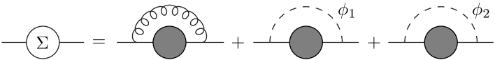
Figure 2: The equation for $\Sigma$.

3 Mesons

3.1 The Bethe-Salpeter equation

Now we want to study $q\,{\bar{q}}$ bound states. In our reduction we have four possible combinations of quark bilinears to describe these states with valence quarks: $(\psi_{a}\,{\bar{\psi}}_{a}),(\psi_{a}\,{\bar{\psi}}_{b}),$ $(\psi_{b}\,{\bar{\psi}}_{a}),(\psi_{b}\,{\bar{\psi}}_{b})$. Each of these bilinears can be, of course, supplemented with a number of gluons and adjoint scalars. Moreover, unlike the t’Hooft model, the interaction in our dimensionally reduced model mixes all sectors of the Fock space with quark, antiquark and any number of scalars, even in the planar limit, as it has been realized before in the light-cone quantization approach [18]. However in the low-energy region for $M^{2}\gg m^{2}_{d}$ one can successfully analyze the deviation from the t’Hooft bound state wave function just retaining the ladder exchange both by gluon and by scalars for calculation of the valence quark wave function and neglecting vertex and self-energy corrections as well as the mixing with hybrid states which are (superficially) estimated to be of higher order in the $1/M^{2}$ expansion. In this approach the $q\bar{q}$ wave functions satisfy the Bethe-Salpeter equation, for example $\psi_{a}\,{\bar{\psi}}_{a}$ satisfies an equation given graphically in fig.3. The Bethe-Salpeter equations for these four states mix them (see fig.3) but if we define the following combinations the equations decouple:

$$\Lambda(p,q)=\frac{1}{2}\left(\Psi_{ab}-\Psi_{ba}\right)\,, \Delta(p,q)=\frac{1}{2}\left(\Psi_{aa}+\Psi_{bb}\right)\,,$$ (37)

$$\Theta(p,q)=\frac{1}{2}\left(\Psi_{ab}+\Psi_{ba}\right)\,, \Omega(p,q)=\frac{1}{2}\left(\Psi_{aa}-\Psi_{bb}\right)\,.$$ (38)

These combinations have a direct interpretation in term of Dirac bilinears of the theory in $(3+1)$ dimensions. In particular, the scalar and pseudoscalar densities, which are within our scope in this paper, can be represented by,

$$S={\bar{\Psi}}\,\Psi=2\,Tr(\Delta)\,,$$ (39)

$$P={\bar{\Psi}}\,\gamma^{5}\,\Psi=-2i\,Tr(\Lambda\,\sigma_{3})\,,$$ (40)

were $\Psi$ is a four dimensional bispinor.

Respectively the manifest form of the Bethe-Salpeter equations on wave functions (37) is:

$$\Lambda(p,q)=iS(p-q)\left(ig\gamma_{-}\right)\!\int\!\frac{d^{2}k}{(2\pi)^{2}}\;\left[\frac{{\bf P}}{(k-q)_{-}^{2}}\,\,\Lambda(p,k)\right]\left(ig\gamma_{-}\right)S(-q)$$

$$-\,2iS(p-q)\left(g\sigma_{3}\right)\!\int\!\frac{d^{2}k}{(2\pi)^{2}}\;\left[\frac{1}{\left[2(p-q)_{+}(p-q)_{-}-M^{2}+i\epsilon\right]}\,\,\Lambda(p,k)\right]\left(g\sigma_{3}\right)S(-q)\,.$$ (41)

$$\Delta(p,q)=iS(p-q)\left(ig\gamma_{-}\right)\!\int\!\frac{d^{2}k}{(2\pi)^{2}}\;\left[\frac{{\bf P}}{(k-q)_{-}^{2}}\,\,\Delta(p,k)\right]\left(ig\gamma_{-}\right)S(-q)$$

$$+\,2iS(p-q)\left(g\sigma_{3}\right)\!\int\!\frac{d^{2}k}{(2\pi)^{2}}\;\left[\frac{1}{\left[2(p-q)_{+}(p-q)_{-}-M^{2}+i\epsilon\right]}\,\,\Delta(p,k)\right]\left(g\sigma_{3}\right)S(-q)\,.$$ (42)

Further on we are going to focus our analysis on these equations to describe scalar and pseudoscalar meson states.

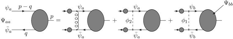
Figure 3: Bethe-Salpeter equation for the state $\Psi_{aa}$. Notice that in this equation the state $\Psi_{bb}$ appears.

3.2 Integral Equation for $\Lambda$ and Pseudoscalar Mesons

Let us explore solutions of the matrix integral equation (41). To do that we decompose the matrix $\Lambda$ as follows:

$$\Lambda(p,q)=\Lambda_{+}\,\gamma_{+}+\Lambda_{-}\,\gamma_{-}+\Lambda_{+-}\,\gamma_{+}\,\gamma_{-}+\Lambda_{-+}\,\gamma_{-}\,\gamma_{+}\,,$$ (43)

then in components Eq.(41) yields four integral equations:

$$\Lambda_{+}(p,q)=\frac{-4i{g}^{2}(p-q)_{-}q_{-}}{D[p-q]\,D[q]}\int\!\frac{d^{2}k}{(2\pi)^{2}}\left[\frac{{\bf P}}{(k-q)_{-}^{2}}\,\,\Lambda_{+}(p,k)\right]$$ (44)

$$+\,\frac{2i{g}^{2}}{D[p-q]\,D[q]}\!\int\!\frac{d^{2}k}{(2\pi)^{2}}\left[\frac{2(p-q)_{-}q_{-}\Lambda_{-}-2q_{-}\,\Sigma_{0}\,\Lambda_{+-}+2\,\Sigma_{0}(p-q)_{-}\Lambda_{-+}-{\Sigma_{0}}^{2}\Lambda_{+}}{\left[(k-q)^{2}-M^{2}+i\epsilon\right]}\right]\,.$$

$$\Lambda_{-}(p,q)=\frac{2i{g}^{2}\,{\Sigma}^{2}_{0}}{D[p-q]\,D[q]}\int\!\frac{d^{2}k}{(2\pi)^{2}}\left[\frac{{\bf P}}{(k-q)_{-}^{2}}\,\,\Lambda_{+}(p,k)\right]$$ (45)

$$+\,\frac{2i{g}^{2}}{D[p-q]\,D[q]}\!\int\!\frac{d^{2}k}{(2\pi)^{2}}\left[\frac{2[p-q][q]\Lambda_{+}-2[q]\,\Sigma_{0}\,\Lambda_{-+}+2\,\Sigma_{0}\,[p-q]\Lambda_{+-}-{\Sigma_{0}}^{2}\Lambda_{-}}{\left[(k-q)^{2}-M^{2}+i\epsilon\right]}\right]\,.$$

$$\Lambda_{+-}(p,q)=\frac{2i{g}^{2}\,{\Sigma}_{0}\,(p-q)_{-}}{D[p-q]\,D[q]}\int\!\frac{d^{2}k}{(2\pi)^{2}}\left[\frac{{\bf P}}{(k-q)_{-}^{2}}\,\,\Lambda_{+}(p,k)\right]$$ (46)

$$+\,\frac{2i{g}^{2}}{D[p-q]\,D[q]}\!\int\!\frac{d^{2}k}{(2\pi)^{2}}\left[\frac{2(p-q)_{-}[-q]\Lambda_{-+}+[q]\,\Sigma_{0}\,\Lambda_{+}-\Sigma_{0}\,(p-q)_{-}\Lambda_{-}+{\Sigma_{0}}^{2}\Lambda_{+-}}{\left[(k-q)^{2}-M^{2}+i\epsilon\right]}\right]\,.$$

$$\Lambda_{-+}(p,q)=-\frac{2i{g}^{2}\,{\Sigma}_{0}\,\,q_{-}}{D[p-q]\,D[q]}\int\!\frac{d^{2}k}{(2\pi)^{2}}\left[\frac{{\bf P}}{(k-q)_{-}^{2}}\,\,\Lambda_{+}(p,k)\right]$$ (47)

$$+\,\frac{2i{g}^{2}}{D[p-q]\,D[q]}\!\int\!\frac{d^{2}k}{(2\pi)^{2}}\left[\frac{-2[p-q]q_{-}\Lambda_{+-}+q_{-}\,\Sigma_{0}\,\Lambda_{-}-\Sigma_{0}\,[p-q]\Lambda_{+}+{\Sigma_{0}}^{2}\Lambda_{-+}}{\left[(k-q)^{2}-M^{2}+i\epsilon\right]}\right]\,,$$

where we have defined $D[q]=q^{2}-m^{2}_{d}+i\epsilon$, and $[q]=q_{+}+\frac{g^{2}}{2\pi}\left(\frac{{\bf P}}{q_{-}}\right)$.

In order to have control over the expansion in $\frac{1}{M^{2}}$ let us introduce the following variables:

$${\bar{\Lambda}}_{-}(p,q)=-2\frac{(p-q)_{-}\,q_{-}}{\Sigma^{2}_{0}}\,\Lambda_{-}(p,q)+\Lambda_{+}(p,q)\,, {\bar{\Lambda}}_{+-}(p,q)=-2\frac{q_{-}}{\Sigma^{2}_{0}}\,\Lambda_{+-}(p,q)+\Lambda_{+}(p,q)\,,$$

$${\bar{\Lambda}}_{-+}(p,q)=2\frac{(p-q)_{-}}{\Sigma^{2}_{0}}\,\Lambda_{-+}(p,q)+\Lambda_{+}(p,q)\,.$$ (48)

One can see that in the large $M^{2}$ limit the equations for these new variables contain only terms, superficially proportional to $\frac{1}{M^{2}}$. Meantime the equation for $\Lambda_{+}$ contains ’t Hooft operator (which is of zero order in $\frac{1}{M^{2}}$) as well as the terms of order $\frac{1}{M^{2}}$ in which both the new variables and also $\Lambda_{+}$ appear. Since the corrections to the ’t Hooft equation for $\Lambda_{+}$ are examined here at the leading order in $\frac{1}{M^{2}}$ expansion, we retain in this equation only the terms including $\Lambda_{+}$:

$$\Lambda_{+}(p,q)=2ig^{2}\,\frac{(p-q)_{-}\,q_{-}}{D[p-q]\,D[q]}\left[-2\int\!\frac{d^{2}k}{(2\pi)^{2}}\frac{{\bf P}}{(k-q)_{-}^{2}}\,\,\Lambda_{+}(p,k)\right.$$ (49)

$$-\Sigma_{0}^{2}\int\!\frac{d^{2}k}{(2\pi)^{2}}\frac{1}{(p-k)_{-}\,k_{-}}\,\frac{\Lambda_{+}(k)}{\left[(k-q)^{2}-M^{2}+i\epsilon\right]}-\frac{\Sigma_{0}^{2}}{(p-q)_{-}\,q_{-}}\int\!\frac{d^{2}k}{(2\pi)^{2}}\,\frac{\Lambda_{+}(k)}{\left[(k-q)^{2}-M^{2}+i\epsilon\right]}$$

$$\left.+\,\frac{\Sigma^{2}_{0}}{(p-q)_{-}}\int\!\frac{d^{2}k}{(2\pi)^{2}}\frac{1}{k_{-}}\,\frac{\Lambda_{+}(k)}{\left[(k-q)^{2}-M^{2}+i\epsilon\right]}+\,\frac{\Sigma^{2}_{0}}{q_{-}}\int\!\frac{d^{2}k}{(2\pi)^{2}}\frac{1}{(p-k)_{-}}\,\frac{\Lambda_{+}(k)}{\left[(k-q)^{2}-M^{2}+i\epsilon\right]}\right].$$

In the region $(k-q)^{2}\ll M^{2}$ one can integrate over $q_{+}$ on both sides of equation (49), obtaining the following integral equation for the eigenvalues $p^{2}$:

$$\left[p^{2}-\frac{m^{2}_{d}}{x}-\frac{m^{2}_{d}}{(1-x)}\right]\phi(x)=\,-\frac{g^{2}}{\pi}\,\int^{1}_{0}\!dy\,\frac{{\bf P}}{(x-y)^{2}}\,\,\phi(y)-\,A\,\frac{\Sigma^{2}_{0}}{x^{1-\beta}}\int^{1}_{0}\!dy\,\frac{\phi(y)}{(1-y)^{1-\beta}}$$

$$-\,A\,\frac{\Sigma^{2}_{0}}{(1-x)^{1-\beta}}\int^{1}_{0}\!dy\,\frac{\phi(y)}{y^{1-\beta}}+\,A\,\frac{\Sigma^{2}_{0}}{[(1-x)\,x]^{1-\beta}}\int^{1}_{0}\!dy\,\phi(y)+\,A\,\Sigma^{2}_{0}\,\int^{1}_{0}\!dy\,\frac{\phi(y)}{[(1-y)\,y]^{1-\beta}}\,.$$ (50)

Where we have conventionally introduced $\phi(q_{-})=\int dq_{+}\,\Lambda_{+}$ and dimensionless variables $q_{-}=xp_{-}$, $k_{-}=yp_{-}$ as well as the expansion parameter $A$, previously defined in Eq.(13). The integral equation (50) has a symmetric kernel that guarantees that the eigenvalues $p^{2}$ are real. It is also symmetric under the transformation $x\rightarrow(1-x)$ found by ’t Hooft in [2].

To the first order in $A$ the straightforward calculation from Eq.(49) gives $\beta=0$, but such a kernel makes this equation too singular to have any reasonable solutions. This singularity must be softened by re-summation of a series of similar singularities of higher order in $A$. Just in order to simulate this re-summation we have introduced $\beta$ which effectively regularize the integral equation. The coefficient $\beta$ governs the behavior of the solution of Eq.(50) near the end points. We fix it by imposing self consistency of solutions near the boundaries. Although the parameter $\beta$ is small and vanishing with $A\rightarrow 0$, its presence guarantees the positivity of the spectrum (see appendix B).

4 Integral Equation and Approximate Spectrum

To explore solutions to Eq.(50) we examine small $A$, which allows us to put $m^{2}_{d}=0$. Working in this limit we select out consistently the wave functions that behave as $x^{\beta}$ or $(1-x)^{\beta}$ on the boundaries, then $\beta$ is fixed to $\frac{A}{2}$ in order to cancel the principal divergences, $x^{\beta-1}$ and $(1-x)^{\beta-1}$, that appear when $x$ is near the end points.

Evidently Eq.(50) does not mix even and odd functions with respect to the symmetry $x\Longleftrightarrow 1-x$. On the other hand the ground state should be an even function. When inspecting the wave function end-point asymptotics from the integral equation (50) one derives the following even function as a ground state solution for $A\rightarrow 0$ limit:

$$\phi_{0}(x)=(4x[1-x])^{\frac{A}{2}}-\frac{1}{\pi}\,(4x[1-x])^{\frac{1}{2}}\,.$$ (51)

This is basically a non-perturbative result that differs from ’t Hooft solution in the $A\rightarrow 0$ limit, giving $p^{2}=0$, as we would expect from spontaneous chiral symmetry breaking in $4D$. Notice that the second term in Eq.(51) is a leading contribution to the ground state solution for ’t Hooft equation with $m^{2}=\frac{g^{2}}{\pi}$ [2], and the first term compensates powers of $A$ when we insert $\phi_{0}(x)$ in Eq.(50) and take the $A\rightarrow 0$ limit. The entire result is a shift of the “unperturbed” ground state $p^{2}=7.25\frac{g^{2}}{\pi}$ (just the ’t Hooft solution with $m^{2}=\frac{g^{2}}{\pi}$) to the non-perturbative solution with $p^{2}=0$ in the $A\rightarrow 0$ limit. For the other massive states we are unable to find analytic solutions, as happens with ’t Hooft equation, but we could estimate them working with the Hamiltonian matrix elements $p^{2}(\phi,\phi)=(\phi,H\phi)$ and using the regular perturbation theory, starting from ’t Hooft solutions ($A=0$) [2]. Formally the set of solutions to Eq.(50) is composed of even and odd functions with respect to the reflection $x\Longleftrightarrow 1-x$, but only the even functions have physical meaning as describing pseudoscalar states. It occurs because the $4D$ pseudoscalar density could be written as a combination of $2D$ pseudoscalar densities for which it is possible to use the arguments given in [3]. Thus for the pseudoscalar sector only the set of even solutions of Eq.(50) is selected out. Similarly for scalar states the equation differs from Eq.(50) by signs of perturbation terms, i.e. $A\longrightarrow-A$ and the appropriate set of solutions consists of odd functions, then only perturbative massive solutions are possible for these states. As we have significantly departed from $QCD_{4}$ neglecting heavy K-K states and taking the limit $A\rightarrow 0$ we don’t make any numerical fits to some observable mesons with quantum numbers of scalar and pseudoscalar radial excitations just postponing this work till a more systematic estimations of neglected terms.

5 Conclusions

We summarize our points. Quantum Chromodynamics at low energies has been decomposed by means of dimensional reduction from $(3+1)$ to $(1+1)$ dimensions and a low energy effective model in $2D$ has been derived. It is presumably more realistic than just taking QCD in $2D$ because the model includes, in a nontrivial way, physical (transverse) gluon degrees of freedom. We treat this model in the equal-time quantization approach using Schwinger-Dyson equations instead of Hamiltonian quantization, and we argued that the adjoint scalar fields dynamically gain masses. We did an explicit analysis of the meson bound states by using Bethe-Salpeter equation in the limit of large scalar masses.

We found that the model has two regimes classified by the solutions of quark self-energy. In one case, the perturbative one, we have tachyonic quarks in the chiral limit as in [2] and our model could be interpreted as a perturbation from the result of chiral QCD in $2D$. But we are not allowed to consider that possibility because the spectrum for the lowest $q{\bar{q}}$ bound states becomes imaginary once we consider small but nonzero $A$, see appendix A. This means that the ’t Hooft chiral solution is not a stable background to start a perturbation to $QCD_{2}$ that includes transverse degrees of freedom. Also in this regime the equations that describe the mass spectrum for scalars and pseudoscalars are equal, certainly we have oversimplified something. On the other hand the non-perturbative solution to quark self-energy supports non-tachyonic quarks with masses going to zero, in the chiral limit.

We focused our attention on bound states of quark-antiquark in the valence quark approximation which is right for low energies. It was shown that $q{\bar{q}}$ states constructed in our reduced model have a direct interpretation in terms of their properties under Lorentz transformations inherited from $(3+1)$ dimensions. Respectively, we have different equations that govern the scalar and pseudoscalar mass spectrum and in both cases the spectrum is positive definite with a massive ground state for scalars and a massless ground state for pseudoscalars.

The pseudoscalar and scalar sectors of the theory have been analyzed and a massless solution for the pseudoscalar ground state has been found. We interpreted this solution as a “pion” of our model although it is a quantum mechanical state only existing in the large-$N_{c}$ limit. The appearance of massless boson in a two dimensional theory in a particular limit is not a new feature and has been studied in [25, 9, 13] and more recently justified in [26]. In particular in the planar $QCD_{2}$ the ’t Hooft pion solution is a massless boson bound state, related with a non-anomalous $U(1)$ symmetry. We expect that our pion solution Eq.(51) has more physical properties from the $4D$ theory, as compared to the massless solution of QCD $2D$. For the latter one, it has been proved that the ’t Hooft pion state is decoupled from the rest of the states [16]. On the contrary, the argument of non-anomalous $U(1)$ symmetry that produced the decoupling of the massless scalar field in $QCD_{2}$ does not hold in our model.

Indeed in $QCD_{2}$ the $U(1)$ vector current $J^{\mu}={\bar{\psi}}^{a}\gamma^{\mu}\psi^{a}+{\bar{\psi}}^{b}\gamma^{\mu}\psi^{b}$ is conserved then $J^{\mu}=\epsilon^{\mu\,\nu}\partial_{\nu}\phi(x)$. Due to $\gamma_{\mu}\,\gamma_{5}=\epsilon_{\mu\,\nu}\gamma^{\nu}$ we can write the $U(1)$ axial current as follows $J^{5}_{\mu}=\partial_{\mu}\phi(x)$, then if the axial current is also conserved we have $\partial^{\mu}\partial_{\mu}\phi=0$, a massless decoupled scalar field. This scalar field is identified with the $\phi_{0}=1$ ’t Hooft state.

In our model the situation is different because the $U(1)$ axial symmetry is explicitly broken by the interaction term in Eq.(2.2), but our model has another symmetry due to the breakdown of the $4D$ Lorentz symmetry $SO(1,3)$ to $SO(1,1)\times O(2)$, where $O(2)$ now becomes an internal symmetry. The vector and axial currents associated with this symmetry are conserved and the axial symmetry corresponds precisely to the projection of the $U(1)$ axial symmetry in $4D$ to our model in $2D$. Our massless pseudoscalar meson is related with these currents, then we cannot expect the same behavior for our massless pseudoscalar as in $QCD_{2}$ because we are talking about different symmetries. For instance, the vector and axial $O(2)$ currents do not satisfy the same relation as $J_{\mu}$ and $J_{\mu}^{5}$ in $QCD_{2}$. On the other hand the possibility to have a coupled massless scalar in the large-$N_{c}$ does not contradict the Coleman theorem as it has been first pointed out in [25], and particular in our case because it is not a quantum Goldstone field but a quantum-mechanical state. We stress that this composite massless state can be related to the real pion, to some extent, at the tree level as the chiral $2D$ perturbation theory being renormalizable is drastically different from the $QCD$ $4D$ Ch.P.T. [27].

Appendix A Quark-Self Energy, First Solution

Let us consider the t’Hooft solution for the quark self energy $\chi_{+}=\frac{i}{2\pi}\frac{g^{2}}{p_{-}}$, $\chi_{0}=0$ and $\chi_{-}=0$ and explore what this solution implies for the bound state spectrum of quarks and antiquarks. We proceed in the same way as before obtaining a similar Bethe-Salpeter (BS) equation for $\Lambda(p,q)$ Eq.(41), but now the dynamic mass is the one found in [2] ($m^{2}_{d}=m^{2}-\frac{g^{2}}{\pi}$) and $\Sigma_{0}$ is zero. In the chiral limit ($m=0$), we write the BS equation in terms of the decomposition given in Eq.(43) and obtain two decoupled sets of equations: one for $\Lambda_{+}(p,q)$ and $\Lambda_{-}(p,q)$ and the other one for $\Lambda_{+-}(p,q)$ and $\Lambda_{-+}(p,q)$. To calculate corrections to the ’t Hooft equation for $\Lambda_{+}$ we retain just the first set of equations:

$$\Lambda_{+}(p,q)=\frac{-4i{g}^{2}(p-q)_{-}q_{-}}{D[p-q]\,D[q]}\Bigg{[}$$ (52)

$$\int\!\frac{d^{2}k}{(2\pi)^{2}}\frac{{\bf P}}{(k-q)_{-}^{2}}\,\,\Lambda_{+}(p,k)-\!\int\!\frac{d^{2}k}{(2\pi)^{2}}\frac{\Lambda_{-}(p,k)}{\left[(k-q)^{2}-M^{2}+i\epsilon\right]}\Bigg{]},$$

$$\Lambda_{-}(p,q)=\frac{4i{g}^{2}\,[p-q][q]}{D[p-q]\,D[q]}\!\int\!\frac{d^{2}k}{(2\pi)^{2}}\frac{\Lambda_{+}(p,k)}{\left[(k-q)^{2}-M^{2}+i\epsilon\right]},$$ (53)

where we can write $[q]=\frac{1}{2}(q^{2}-m^{2}_{d})\left(\frac{{\bf P}}{q_{-}}\right)$. Then the equation for $\Lambda_{-}(p,q)$ becomes:

$$\Lambda_{-}(p,k)=i{g}^{2}\,\left(\frac{{\bf P}}{k_{-}}\right)\left(\frac{{\bf P}}{(p-k)_{-}}\right)\!\int\!\frac{d^{2}k^{\prime}}{(2\pi)^{2}}\frac{\Lambda_{+}(p,k^{\prime})}{\left[(k-k^{\prime})^{2}-M^{2}+i\epsilon\right]},$$ (54)

now we replace this equation into Eq.(52) and integrate over $k$ in the second term retaining only the first $\frac{g^{2}}{M^{2}}$ order. Further on, it is possible to integrate over $q_{+}$ at both sides of the equation obtaining the following integral equation for $\phi(x)$:

$$\left[{\bar{p}}^{2}+\frac{1}{x(1-x)}\right]\phi(x)=-\int^{1}_{0}\!dy\,\frac{{\bf P}}{(x-y)^{2}}\,\,\phi(y)$$

$$+\,A\int^{1}_{0}\!dy\frac{{\bf P}}{(x-y)}\,\ln\left(\frac{(1-x)\,y}{(1-y)\,x}\right)\phi(y),$$ (55)

where we have defined ${\bar{p}}^{2}=\frac{\pi}{g^{2}}p^{2}$. One might solve this equation by using perturbation theory near ’t Hooft solution ($A=0$). We know from [2] that the ground state of ’t Hooft equation is $\phi_{0}(x)=1$ with ${\bar{p}}^{2}=0$, but the perturbation term in Eq.(55) generates a negative correction to ${\bar{p}}^{2}$. Thereby for non-zero values of $A$ we obtain for the ground state an imaginary mass.

Appendix B Positivity of the Spectrum

Here we show that the spectrum of integral equation (50) is indeed positive as stated above. We know that the lowest state should be an even function. For any function that goes to zero faster than $x^{\frac{A}{2}}$ or $(1-x)^{\frac{A}{2}}$ when $x$ goes to zero or one, respectively, we can consider the terms proportional to $A$ as perturbations to ’t Hooft term which is positive definite. Then the only possible trial functions that could generate negative $p^{2}$ are nearly constant functions. Let us explore this possibility and consider a function $f(x)=[x(1-x)]^{\gamma}$, with $\gamma$ small but arbitrary, then we multiply both sides of Eq.(50) by $f(x)$ and integrate over $x$ obtaining (see appendix of reference [24]):

$${\bar{p}}^{2}\langle f(x)|f(x)\rangle=2^{4\gamma-2}\,\gamma\,\frac{\Gamma[\gamma]^{4}}{\Gamma[2\gamma]^{2}}-2A\pi\,\frac{\Gamma[\gamma+\beta]^{2}}{\Gamma[\frac{1}{2}+\gamma+\beta]^{2}}+2A\pi\,\frac{\Gamma[\gamma+\beta]\,\Gamma[1+\gamma]}{\Gamma[\frac{1}{2}+\gamma+\beta]\,\Gamma[\frac{3}{2}+\gamma]}\,.$$ (56)

If we assume $A$ and $\gamma\equiv\alpha A$ to be small, only the first two terms of the right hand side of Eq.(56) are relevant. The divergent part of Eq.(56) is:

$${\bar{p}}^{2}\langle f(x)|f(x)\rangle\sim\frac{1}{\gamma}\left[1-\frac{2A\gamma}{(\gamma+\beta)^{2}}\right]=\frac{1}{\gamma}\left[1-\frac{2\alpha}{(\alpha+\frac{1}{2})^{2}}\right].$$ (57)

Then for any value of $\alpha$ the expression between brackets is evidently positive.

Notice that the existence of a non-zero $\beta$ guarantees the positivity of the spectrum, when $\gamma$ goes to zero and $A$ is small but different from zero.

References

• [1] G. ’t Hooft, Nucl. Phys. B72 (1974) 461.
• [2] G. ’t Hooft, Nucl. Phys. B75 (1974) 461.
• [3] C. Callan, Jr., N. Coote and D. Gross, Phys. Rev. D13 (1976) 1649.
• [4] M. Einhorn, Phys. Rev. D14 (1976) 3451; M. Einhorn, S. Nussinov and E. Rabinovici, Phys. Rev. D15 (1977) 2282; M. Bishary, Ann. Phys. (N.Y.) 129 (1980) 435.
• [5] R. Brower, J. Ellis, M. Schmidt and J. Weis, Nucl. Phys. B128 (1977) 131.
• [6] C. Callan, R. Dashen, D. Gross, Phys. Rev. D16 (1977) 2526; J. Ellis, Y. Frishman, A. Hanany and M. Karliner, Nucl. Phys. B382 (1992) 189.
• [7] A. Bassetto, L. Griguolo and F. Vian, Nucl. Phys. B559 (1999) 563.
• [8] D. Gepner, Nucl. Phys. B252 (1985) (481); G. Date, Y. Frishman and J. Sonnenschein, Nucl. Phys. B283 (1987) 365.
• [9] A. Zhitnitsky, Phys. Lett. B165 (1985) 405; B. Chibisov and A. Zhitnitsky, Phys. Lett. b362 (1995) 105; A. Zhitnitsky, Phys. Rev. D53 (1996) 5821.
• [10] I. Bigi, M. Shifman, N. Uraltsev and A. Vainshtein, Phys. Rev. D59 (1999) 054011.
• [11] P. Steinhardt, Nucl. Phys. B176 (1980) 100.
• [12] I. Affleck, Nucl. Phys. B265 (1985) 448.
• [13] A. Ferrando and V. Vento, Phys. Lett. B256 (1991) 503; A. Ferrando and V. Vento, Phys. Lett. B265 (1991) 153.
• [14] A. Ferrando and V. Vento, Z. Phys. C58 (1993) 133.
• [15] D. Gross, Nucl. Phys. D400 (1993) 161; D. Gross and W. Taylor, Nucl. Phys. D400 (1993) 181; M.R. Douglas and V.A. Kazakov, Phys. Lett. B319 (1993) 219.
• [16] W. Krauth and M. Staudacher, Phys. Lett. B388 (1996) 808.
• [17] S. Dalley and I.R. Klebanov, Rhys. Rev. D47 (1993) 2517; S. Dalley and I.R. Klebanov, Phys. Lett. B298 (1993) 79.
• [18] H.-C. Pauli and S.J. Brodsky, Rhys. Rev. D32 (1985) 1993 and 2001; F. Antonuccio and S. Dalley, Phys. Lett. B376 (1996) 154.
• [19] Y. Hosotani, Phys. Lett. B126 (1983) 309; Y. Hosotani, Ann. Phys. 190 (1989) 233.
• [20] A similar particle content in $2D$ was set in the extended $QCD_{2}$ model treated under the light-cone quantization [18]. However this quantization leads to the trivial QCD vacuum and has difficulties to describe such crucial nonperturbative phenomena as infrared mass generation for transverse gluons and the spontaneous chiral symmetry breaking.
• [21] S. Coleman, Comm. Math. Phys. 31 (1973) 461.
• [22] S. Coleman, $\frac{1}{N}$, in Aspect of Symmetry, Cambridge University Press, Cambridge, 1985.
• [23] M. Burkardt, Phys. Rev. D56 (1997) 7105.
• [24] K. Harada, T. Sugihara, M. Taniguchi and M. Yahiro, Phys. Rev. D49 (1994) 4226.
• [25] E. Witten, Nucl. Phys. B145 (1978) 110.
• [26] M. Faber and A. Ivanov, Eur. Phys. J. C24 (2002) 653.
• [27] J. Gasser and H. Leutwyler, Annals Phys. 142 (1984) 142;