Aspects of Stability and Phenomenology in Type IIA Orientifolds with Intersecting D6-branes

Tassilo Ott

Humboldt–Universität zu Berlin, Institut für Physik
Newtonstraße 15, D-12489 Berlin, Germany
e-mail: ott@physik.hu-berlin.de

Abstract

Intersecting branes have been the subject of an elaborate string model building for several years. After a general introduction into string theory, this work introduces in detail the toroidal and $\mathbb{Z}_{N}$-orientifolds. The picture involving D9-branes with B-fluxes is shortly reviewed, but the main discussion employs the T-dual picture of intersecting D6-branes. The derivation of the R-R and NS-NS tadpole cancellation conditions in the conformal field theory is shown in great detail. Various aspects of the open and closed chiral and non-chiral massless spectrum are discussed, involving spacetime anomalies and the generalized Green-Schwarz mechanism. An introduction into possible gauge breaking mechanisms is given, too. Afterwards, both $\mathcal{N}$=1 supersymmetric and non-supersymmetric approaches to low energy model building are treated. Firstly, the problem of complex structure instabilities in toroidal $\Omega R$-orientifolds is approached by a $\mathbb{Z}_{3}$-orbifolded model. In particular, a stable non-supersymmetric standard-like model with three fermion generations is discussed. This model features the standard model gauge groups at the same time as having a massless hypercharge, but possessing an additional global $B$-$L$ symmetry. The electroweak Higgs mechanism and the Yukawa couplings are not realized in the usual way. It is shown that this model descends naturally from a flipped $SU(5)$ GUT model, where the string scale has to be at least of the order of the GUT scale. Secondly, supersymmetric models on the $\mathbb{Z}_{4}$-orbifold are discussed, involving exceptional 3-cycles and the explicit construction of fractional D-branes. A three generation Pati-Salam model is constructed as a particular example, where several brane recombination mechanisms are used, yielding non-flat and non-factorizable branes. This model even can be broken down to a MSSM-like model with a massless hypercharge. Finally, the possibility that unstable closed and open string moduli could have played the role of the inflaton in the evolution of the universe is being explored. In the closed string sector, the important slow-rolling requirement can only be fulfilled for very specific cases, where some moduli are frozen and a special choice of coordinates is taken. In the open string sector, inflation does not seem to be possible at all.

Chapter 1 Introduction

At the turn of the new century, the physical community suffers from a similar crisis in spirit as it already did 100 years ago. At that time, an older professor advised Planck against studying physics, because the foundation of physics would be complete. There would be not much to discover anymore as all observations would have been explained already [1]. Nevertheless, it was a great fortune that Planck still decided to study physics. Indeed, some years after this unedifying statement, the most exciting developments in physics so far, general relativity and quantum mechanics, have taken place. Today, the situation is quite similar: there are two phenomenological models that seem to describe all empirical observations.

On the first hand, there is the standard model of particle physics, which describes the microscopic structure of our world very well, i.e. the observations that are done in particle colliders up to the current limit of approximately 200 GeV. This model is based on quantum field theory with gauge groups $SU(3)\times SU(2)\times U(1)$. It has been discovered directly from experiment and in its complex structure not just from fundamental principles. There are 18 or more free parameters (depending on the way of counting) [2] in this model, just to mention the masses of the fermions and bosons, the coupling constants of the interactions and the coefficients of the CKM-matrix. These parameters have to be measured, they cannot be determined within the model. But there are even more open questions: for instance, why are there exactly three families of fermions? What is the reason for CP-violation?

On the other hand, there is the standard model of cosmology which describes the macroscopic structure of the universe today successfully, the galaxy formations and the global evolution of the universe by the Hubble parameter. It is built on general relativity combined with simple Hydrodynamics. But this model has its problems, too. There are the Horizon and Flatness problems and the small value of the Cosmological Constant, the last two problems requiring an incredible finetuning of the parameters within the model. These problems in the past have been addressed by theories like inflation or quintessence which slightly alter the phenomenological model but do not touch the underlying theory of general relativity. But there are even more fundamental shortcomings: one cannot determine the values for the Hubble parameter from the model itself, it again is an input parameter. Furthermore, if we interpolate the evolution of the universe back in time, we reach a point at which the thermal energy of typical particles is such that their de Broglie wavelength is equal or smaller than their Schwarzschild radius. This energy is the Planck mass $M_{P}=1.22\times 10^{19}$ GeV. It means nothing else than the breakdown of general relativity at least at this scale, because it relies on a smooth spacetime which would be destroyed by quantum black holes.

This fact can be seen as a hint that neither quantum mechanics (quantum field theory) nor general relativity on their own can describe what has happened at the beginning of our universe. From the philosophical point of view this maybe is the deepest question physics might ever be able to answer. This inability within the physical community motivated the idea that all physics might be described by just one fundamental theory that unifies general relativity and quantum field theory as its effective low energy approximations.

1.1 A unification of all fundamental forces

Albert Einstein has started the program of searching for a unified field theory more than 60 years ago [3]. Learning from Maxwells ideas that the electric and magnetic forces are just two different appearances of one unified force, he concluded that this might be also true for all other fundamental forces. At his time, only the gravitational force was known in addition to the electro-magnetic one. He extended the idea of Kaluza [4] from 1921 and Klein [5] from 1926 that within a 5-dimensional classical field theory with one compact direction, gravity could be understood as given by the 4-dimensional part of the metric tensor $g_{\mu\nu}$ with $\mu,\nu=0..3$ and the compact subspace contributing the massless photon as $g_{\mu 4}$. This theory later was discarded, mainly because it predicted a new and unseen massless particle, given by $g_{44}$. At the latest, when the weak and strong forces were discovered, it has become apparent that this imaginative idea has failed in its original formulation.

Unification can generally be understood in two different ways that have to be distinguished carefully. Firstly, one could mean a description of nature within the same theoretical framework. This has indeed been achieved for the three forces excluding gravity by the standard model of particle physics within the framework of quantum field theory. The story is different considering gravitation which is not quantizable, i.e. renormalizable, within four-dimensional quantum field theory.

Secondly, by the term unification in a strong sense one could mean that above a certain energy scale, the different forces dissolve into just one fundamental one. For the electro-magnetic and weak forces this was first achieved in the Salam-Weinberg model which already is included within the standard model. It predicts an electroweak phase transition which should have occurred at an energy of approximately 300 GeV [6] and has helped to understand how our present matter has formed during the cosmological evolution. But a direct evidence for the Higgs particle, triggering this phase transition within the standard model, still is missing. For the three forces without gravity, unification in this sense is achieved in grand unification models. Gauge coupling unification happens at a high energy, the so-called GUT-scale of around $10^{16}$ GeV in typical models. The three standard model gauge groups are getting replaced by one larger simple group. The initial non-supersymmetric $SU(5)$ model has been ruled out. This is due to the predicted proton decay that does not happen, as Super Kamiokande has observed up to a limit $\tau=4.4\times 10^{33}$ years [7, 8]. But there are other models like $SO(10)$ with a larger gauge group that still might give the right description of a electroweak-strong unification, although there are many open questions regarding the Higgs sector or the weak mixing angle that cannot be answered correctly by these models so far.

Another important idea related to unification has entered particle physics within the last thirty years: supersymmetry. It assumes a fundamental symmetry between fermions and bosons, one can be transferred into the other by an operator $Q$ that is called supercharge. This idea has its origin in string theory but was transferred by Wess and Zumino even to 4-dimensional field theory [9, 10]. Supersymmetry predicts a superpartner for every particle. But such superpartners of the standard model particles have not yet been observed in accelerator experiments. This means that at least below 200 GeV, supersymmetry has to be broken, leading to a mass split between the bosonic and fermionic partners that roughly is of the order of the SUSY breaking scale. The additional light particles above this scale in a specific and phenomenologically most favored supersymmetric model, called the MSSM (Minimal Supersymmetric Standard Model), imply (in analogy to GUT models) a unification of the three couplings at a scale that might be around $10^{16}$ GeV, see for instance [11]. Therefore, one of the main challenges of the LHC (Large Hadron Collider), which is being built at CERN right now and is going to achieve center of mass energies of up to 14 TeV, will be the search for supersymmetry. It is even possible to build supersymmetric algebras with more than one superpartner for every particle, this is generally called extended supersymmetry. But it is phenologically disfavored because it does not allow chiral gauge couplings like in the standard model.

Due to its non-renormizability in four dimensions, the unification with gravity in both senses still seems to be a much more difficult problem. Indeed, there is just one prominent candidate for a unifying theory: string theory. It unifies gravity with the other forces within the same theoretical framework, not as one unified force as in the second meaning of the word.

1.2 String theory

String theory [12, 13, 14, 15, 16] manages to undergo the strong divergences of graviton scattering amplitudes in field theory by replacing the concept of point particles by strings. These strings are mathematical one-dimensional curves that spread out a two-dimensional worldsheet $\Sigma$ (which usually is parameterized by the two variables $\sigma$ and $\tau$) when propagating in a higher dimensional spacetime. The string has a characteristic length scale of $\sqrt{\alpha^{\prime}}$, where $\alpha^{\prime}$ is the Regge slope which is generally believed to be the only fundamental constant of string theory. With this new concept, interaction does not take place at a single point, but is smeared out into a region and is already encoded in the topology of the worldsheet. In order to include interaction, a first quantization is sufficient, which can be performed quite easily. The difference between interaction vertices in field theory and string theory is schematically shown in figure 1.1 for a point particle (or a closed string) that splits into two point particles (or closed strings).

Refer to caption
Figure 1.1: Splitting Interaction of a string compared to the corresponding field theory vertex, a coupling $g_{\mathrm{closed}}$ is assigned to this process.

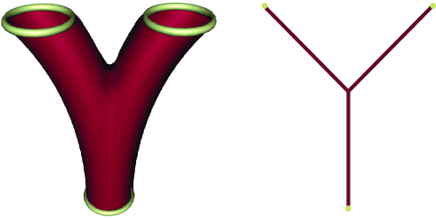
The characteristic energy scale of the string (the string scale) is given by $1/\alpha^{\prime}$. It constitutes the energy at which pure stringy effects should be visible. Surely, this energy must be very high, and for a long time, it was believed to be of the order of the Planck scale [14], but in more recent scenarios sometimes even energies of 1 TeV are favored [17]. At energies much below the string scale (corresponding to the limit $\alpha^{\prime}\rightarrow 0$), the string diagrams (like the left one of figure 1.1) reduce to the usual field theoretic ones (the right one of the same figure).

1.2.1 The bosonic string

On the worldsheet of the bosonic string, there exists a conformal field theory. It is described by the bosonic fields $X^{\mu}(\tau,\sigma)$ with $\mu=0,...,D-1$ and has the action of a non-linear sigma model

(1.1) $$\emph{S}_{\mathrm{Polyakov}}=\frac{1}{4\pi\alpha^{\prime}}\int_{\Sigma}d\tau d\sigma\sqrt{-\gamma}\gamma^{ab}\partial_{a}X^{\mu}\partial_{b}X^{\nu}g_{\mu\nu}\ ,$$

which is called the Polyakov action. Every one of the $D$ massless scalar bosonic fields $X^{\mu}$ has the interpretation of an embedding in a spacetime dimension, in analogy to the point particle which moves in a curved space (with the usual metric tensor $g_{\mu\nu})$. However $\gamma_{ab}$ is the worldsheet metric (where a,b=0,1) that is introduced as an additional field similarly to the tetrad of general relativity. $\gamma_{ab}$ can be eliminated from the action using its algebraic and therefore non-dynamical equation of motion. On the classical level, the Polyakov action has the following three symmetries:

  1. 1.

    $D$-dimensional Poincaré invariance

  2. 2.

    2-dimensional Diffeomorphism invariance

  3. 3.

    2-dimensional Weyl invariance

The Poincaré invariance is similar to that of usual special relativity, in this case extended to all $D$ spacetime dimensions. Diffeomorphism invariance is expected from the tetrad formalism of general relativity. The Weyl invariance can be understood as a local rescaling invariance of the worldsheet. It is crucial for the fact that the 2-dimensional field theory on the worldsheet is conformal.

Strings generally can be open or closed, corresponding to different boundary conditions. In particular, for closed strings the boundary conditions for the $X^{\mu}$ are periodic and so the string forms a closed loop of length $l$:

(1.2) $$X^{\mu}(\tau,l)=X^{\mu}(\tau,0)\ ,\qquad\partial^{\sigma}X^{\mu}(\tau,l)=\partial^{\sigma}X^{\mu}(\tau,0)\ ,\qquad\gamma_{ab}(\tau,l)=\gamma_{ab}(\tau,0)\ .$$

By way of contrast, for open stings the endpoints of the string are not being identified. Consequently, there are boundaries in the conformal field theory:

(1.3) $$\partial^{\sigma}X^{\mu}(\tau,0)=\partial^{\sigma}X^{\mu}(\tau,l)=0\ .$$

These are Neumann boundary conditions and they are the only possibility if we insist on $D$-dimensional Poincaré invariance. Elsewhere an unwanted surface term would be introduced in the variation of the action.

By using the simplest method of quantization for the theory, the light cone quantization, one spatial degree of freedom and the time are getting eliminated in the gauge fixed theory. This is because the string is extended in one spatial direction. As a consequence, not all spacial dimensions in spacetime can be independent, just the transversal ones can oscillate.

In the process of quantization, another restriction arises by the demand of a vanishing Weyl quantum anomaly: the total number of dimensions must be $D=26$, the so-called critical dimension. If one tries to define a meaningful quantum theory using strings, this is the most severe break with usual quantum field theory.111There is a close relation between a non-vanishing Weyl anomaly on the worldsheet and a loss of Lorentz invariance in spacetime which surely is unacceptable, see for instance [14].. Hence one has to think about the question, why the world that we observe is at least effectively 4-dimensional. We will soon return to this question.

The transversal oscillation modes on the string describe particles in the usual sense. We want to describe them now in some more detail:

One obtains a tachyon in both the closed and open string at the lowest mass level, a particle with negative mass-squared. This indicates in field theories that the vacuum, around which one perturbs, is unstable. The same conclusion has been drawn for the bosonic string: it is not a viable theory as it stands.

At the next mass level, one gets the zero-modes of $X^{\mu}$ which correspond to massless bosonic fields in spacetime. In the closed string, there are $(D-2)^{2}$ massless states forming a traceless symmetric tensor, an antisymmetric tensor and a scalar. The traceless symmetric tensor has been interpreted as the graviton by Scherk and Schwarz in 1974 [18, 19]. This lead to the big boom of string theory, because it was the first quantum theory that seemed to naturally incorporate a massless spin-2 particle. In the open string, one obtains a (D-2) massless vector particle.

Furthermore, there is an infinite tower of massive states that are organized in units of the string scale $\alpha^{\prime-1/2}$. Even the lowest one of these modes are so heavy that they do not play any important role if the string scale is really of the order of the Planck scale. Therefore, in the rest of this work and generally within phenomenological models, mainly the zero-modes are being regarded as they highly dominate at energies much below the string scale.

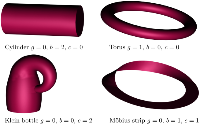
In analogy to quantum field theory, one would like to define a path integral for string theory in order to describe interaction. This then would allow to calculate scattering amplitudes for certain incoming and outgoing string configurations. So far, we have just spoken about one worldsheet with a certain metric $\gamma_{ab}$ and a certain topology. To build up the path integral, one would have to sum over all possible histories that interpolate between the initial and final state. To do so, one first has to classify all the different possible topologies of 2-dimensional Riemann surfaces. This can be done by determining the genus $g$, corresponding to the number of handles and the number of boundaries $b$, corresponding to holes within the surface, and finally the number of crosscaps $c$, corresponding to insertions of projective planes. From these three numbers, the Euler number can be calculated by the simple equation

(1.4) $$\chi=2-2g-b-c\ .$$

In the simplest case of pure closed string theory, there are neither boundaries nor crosscaps, so the perturbative expansion can be directly understood just by the number of handles.

Refer to caption
Figure 1.2: Perturbative expansion for the closed string partition function without insertion.

One assigns a coupling $g_{\mathrm{closed}}=e^{\lambda}$ to the diagram that couples three closed strings (the left figure of 1.1) and then builds up the torus and topologies with more handles by joining two or more of these. Every diagram is then weighed with a factor $e^{-\lambda\chi}$ as can be seen in figure 1.2. This procedure also works for topologies with boundaries or unoriented worldsheets. The Polyakov path integral partition function schematically can be defined in the following way:

(1.5) $$\mathcal{Z}=\sum\limits_{\textrm{all compact topologies}}\int\frac{[dX\ d\gamma]}{V_{\textrm{diff}\times\textrm{Weyl}}}e^{-\mathcal{S(X,\gamma)}-\lambda\chi}\ ,$$

$\mathcal{S(X,\gamma)}$ is the Polyakov action (1.1) and $V_{\textrm{diff}\times\textrm{Weyl}}$ stands for the volume of the string worldsheet symmetry groups that carefully have to be divided out. It is now possible to add asymptotic string states (for instance for calculating the scattering amplitude between one ingoing and two outgoing external closed string states, like in figure 1.1). This is done by adding so-called vertex operators at a certain worldsheet position, one for each external open or closed string state. One carefully has to fix the gauge on every worldsheet topology, because the vertex operators break some of the manifest symmetries. Just to mention, many involved tools from conformal field theory, like operator product expansion, are needed to perform these calculations.

1.2.2 The superstring

Besides the existence of the Tachyon, there is another problem: the theory does not contain any spacetime fermions so far. This can be cured if one adds fermionic degrees of freedom $\psi^{\mu}(\tau,\sigma)$ and enlarges the symmetry algebra by supersymmetry on the worldsheet at the same time. Instead of (1.1), one starts with the Ramond-Neveu-Schwarz action in superconformal gauge:

(1.6) $$\emph{S}_{\mathrm{RNS}}=\frac{1}{4\pi\alpha^{\prime}}\int_{\Sigma}d\tau d\sigma\left(\partial_{\alpha}X^{\mu}\partial^{\alpha}X^{\nu}g_{\mu\nu}+i\bar{\psi}^{\mu}\rho^{\alpha}\partial_{\alpha}\psi_{\mu}\right)\ .$$

The fields $\psi^{\mu}$ are Majorana spinors on the worldsheet, but vectors in spacetime; $\rho^{\alpha}$ are the two-dimensional spin matrices where the worldsheet spinor indices are suppressed. The demand for a vanishing Weyl anomaly leads to a different restriction on the total spacetime dimension as in the bosonic string, and this is $D=10$. The $\psi^{\mu}$ of the open string can have two different periodicities:

(1.7) $\displaystyle\mathrm{Ramond(R)}$ $\displaystyle:\psi^{\mu}(\tau,\sigma+l)=+\psi^{\mu}(\tau,\sigma)$
$\displaystyle\mathrm{Neveu-Schwarz(NS)}$ $\displaystyle:\psi^{\mu}(\tau,\sigma+l)=-\psi^{\mu}(\tau,\sigma)$

The sign must be similar for all $\mu$. If one quantizes the superstring in the same way as the bosonic string, one realizes that the closed string always has two independent left and right moving oscillation degrees of freedom, whereas the open string has just one independent one. For the closed string, it is possible to choose between Ramond and Neveu-Schwarz initial conditions independently for the left and right moving spinors $\psi^{\mu}$ and $\tilde{\psi}^{\mu}$. By doing so, one gets 4 different theories for the closed string (NS-NS, R-R, NS-R and R-NS) and 2 different ones for the open string (NS, R). The theories of NS-NS, R-R and NS yield spacetime bosons, whereas NS-R, R-NS and R account for the spacetime fermions. As explained further down, none of these theories on their own are viable quantum theories, this is mainly due to the demand of modular invariance of the one-loop amplitude and possible non-vanishing tadpoles. Furthermore, some sectors contain a tachyon as the ground state. Gliozzi, Scherk and Olive have shown that it is possible to construct modular invariant, tachyon-free theories from all these sectors. This is done by a certain projection, which today is called GSO-projection [20]. It projects onto states of definite world-sheet fermion number. There are five different string theories known that can be constructed in this way. These are summarized with several properties in table 1.1.

Type Strings Gauge group Chir. SUSY
(10D)
Massless bosonic
spectrum
IIA closed
oriented
U(1)𝑈1U(1) non-
chiral
𝒩𝒩\mathcal{N}=2 NS-NS: gμνsubscript𝑔𝜇𝜈g_{\mu\nu}, ΦΦ\Phi, Bμνsubscript𝐵𝜇𝜈B_{\mu\nu}
R-R:$A_{\mu\nu\rho}$, $A_{\mu}$ in $U(1)$
IIB closed
oriented
none chiral 𝒩𝒩\mathcal{N}=2 NS-NS: gμνsubscript𝑔𝜇𝜈g_{\mu\nu}, ΦΦ\Phi, Bμνsubscript𝐵𝜇𝜈B_{\mu\nu}
R-R:$A$, $A_{\mu\nu}$, $A_{\mu\nu\rho\kappa}$
I open&closed
unoriented
SO(32)𝑆𝑂32SO(32) chiral 𝒩𝒩\mathcal{N}=1 gμνsubscript𝑔𝜇𝜈g_{\mu\nu}, ΦΦ\Phi, Aμνsubscript𝐴𝜇𝜈A_{\mu\nu},
$A_{\mu}$ in Ad[$SO(32)$]
heterotic
SO(32)𝑆𝑂32SO(32)
closed
oriented
SO(32)𝑆𝑂32SO(32) chiral 𝒩𝒩\mathcal{N}=1 gμνsubscript𝑔𝜇𝜈g_{\mu\nu}, ΦΦ\Phi, Bμνsubscript𝐵𝜇𝜈B_{\mu\nu}
$A_{\mu}$ in Ad[$SO(32)$]
heterotic
E8×E8subscript𝐸8subscript𝐸8E_{8}\times E_{8}
closed
oriented
E8×E8subscript𝐸8subscript𝐸8E_{8}\times E_{8} chiral 𝒩𝒩\mathcal{N}=1 gμνsubscript𝑔𝜇𝜈g_{\mu\nu}, ΦΦ\Phi, Bμνsubscript𝐵𝜇𝜈B_{\mu\nu}
$A_{\mu}$ in Ad[$E_{8}\times E_{8}$]
Table 1.1: The five known consistent string theories in $D=10$.

It is possible to build a consistent theory either from just closed strings (type II or heterotic) or from closed plus open strings (type I). In contrast to this, it is not possible to build an interacting theory just from open strings.222A heuristic argument for this fact is that the joining interaction of two open strings locally cannot be distinguished from the joining of the two sides of just one open string, but this produces a closed string. To get a phenomenologically interesting theory, one furthermore has to include non-abelian gauge groups into the theory. This is not possible for the type II closed string theories. However, for the open string one can attach non-dynamical degrees of freedom to both ends of the string, the so-called Chan-Paton-factors. The gauge groups are $U(n)$ in the case of a oriented theory and $SO(n)$ or $Sp(n)$ in the unoriented case, but only the case of $SO(32)$ is anomaly free, as a detailed analysis shows. Therefore, one is also forced to include unoriented worldsheets and the resulting theory is called type I. Another possibility to include non-abelian gauge groups is the heterotic string, where a different constraint algebra acts on the left and right movers, spacetime supersymmetry acts only on the right-movers; From the beginning of the 90s, a lot of research effort has been put in these theories, but they seem to have a serious problem: the gravitational and Yang-Mills-couplings are directly related for the heterotic string and this produces a 4-dimensional Planck mass which is about a factor twenty too high. In this work, the heterotic string will not be treated. The superstring theories do not just have worldsheet supersymmetry, but also extended spacetime supersymmetry. In 10 dimension, the number of supercharges for the different theories varies in between 32 for the type II theories and 16 for the other theories, meaning $\mathcal{N}$=2 or $\mathcal{N}$=1 respectively in 10 dimensions.

1.3 Compactification and spacetime supersymmetry

It has to be explained within string theory why there are just four so far observable dimensions. One hint has been given already by Kaluza-Klein theories which assume a fifth compact and indeed very small dimension. The total dimension for the supersymmetric string theories of the last section has been determined to be $D=10$, meaning that if one expands the Kaluza-Klein idea to this case, the compact subspace should have a dimension $D=6$. One furthermore assumes that the spacetime has a product structure of the following type:

(1.8) $$g_{\mu\nu}=\left(\begin{array}[]{cc}g_{ij}^{(4)}&0\\ 0&g_{ab}^{(6)}\\ \end{array}\right)\ ,$$

where $g_{ij}^{(4)}$ is the 4-dimensional metric, ensuring 4-dimensional Poincaré invariance, and $g_{ab}^{(6)}$ the internal metric of the compact subspace. $g_{ab}^{(6)}$ is unknown. One could only hope to conclude some properties from indirect considerations. In general, any kind of compactification conserves a certain amount of spacetime supersymmetries and breaks the others. Phenomenologically, extended supersymmetry in four dimensions is disfavored, as mentioned already. Therefore, one should end up with a theory having $\mathcal{N}$=1 in four dimensions, meaning four conserved supercharges or even with completely broken supersymmetry $\mathcal{N}$=0.

A first and simple try for such a compact space is given by the six-dimensional torus. It can simply be parameterized by six radii $R_{a}$ that are allowed to depend just on the $x_{i}$ of the non-compact subspace. The metric is given explicitly by $g_{ab}^{(6)}=\delta_{ab}{R_{a}}^{2}(x_{i})$. The radii that indeed label different string vacua are a first example of moduli that we will encounter very often in the course of this work. Similarly to Kaluza-Klein compactification, they can be understood as additional spacetime fields. The case of toroidal compactification already shows several important features of more general compactifications: strings can move around the toroidal dimensions, leaving a quantized center-of-mass momentum. The induced spectrum is called the Kaluza-Klein-spectrum and an effect that can be seen in field theory already. But strings can even wind around the compact dimensions several times, they are then described as topological solitons. The major problem of toroidal compactification is that it conserves all supersymmetries and so does not lead to $\mathcal{N}$=1 in the Minkowski-spacetime.

One simple resolution of this problem has been given in [21, 22] by orbifolding the space. Orbifolding is a classical geometrical method that divides out a certain subspace $S$ of the original space $X$ and then makes the transition to the quotient space $X/S$. For instance, $S$ can be a discrete subgroup like $Z_{n}$. A complete classification has been given in [22] for toroidal orbifolds $T^{6}/Z_{n}$. The procedure of orbifolding induces singularities on the original space, which are unwanted. Still one can understand orbifolds as limits of certain smooth manifolds that are called Calabi-Yau manifolds, where the singularities have been resolved by blowing up the fixed points.

Another last but very important phenomenon that generally occurs in toroidal type compactifications shall be mentioned: T-duality. This is a duality that leaves the coupling constants (and therefore the physics) invariant, but exchanges the radius of the compactified dimension with its inverse, or more precisely with

(1.9) $$R\rightarrow R^{\prime}=\frac{\alpha^{\prime}}{R}.$$

Common sense, claiming that a large or small compactified dimension should be related to very different physics, fails within string theory. T-duality also exchanges Kaluza-Klein and winding states. This fact will become very important in the following chapters. T-duality also has an extension to Calabi-Yau manifolds that are of major interest in string theory, this is called mirror symmetry.

A general Calabi-Yau manifold [23] can be obtained by demanding that its compact subspace has to be a manifold of $SU(3)$-holonomy because this leaves a covariantly constant spinor unbroken. This condition in mathematical language can also be expressed as the requirement to have a Ricci-flat and Kähler manifold. The surviving supercharges are the ones that are invariant under the holonomy group, for $SU(3)$ (not a subgroup) this leads to a minimal $\mathcal{N}$=1 supersymmetry for the heterotic and type I string, but to $\mathcal{N}$=2 for the type II theories in four dimensions.

1.4 D-branes

Dp𝐷𝑝Dp-
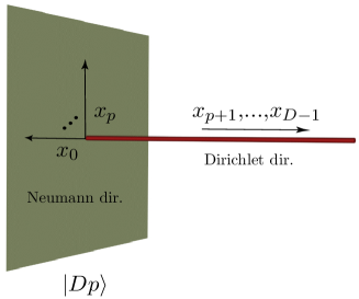
branes fulfill Dirichlet boundary conditions in (Dp1)𝐷𝑝1(D-p-1) directions:

(1.10) $$X^{\mu}(\tau,0)=x^{\mu}_{1}\ ,\qquad X^{\mu}(\tau,l)=x^{\mu}_{2}\qquad\text{for}\ \mu=(p+1),...,(D-1)$$

and Neumann boundary conditions in the remaining $(p+1)$ directions:

(1.11) $$\partial^{\sigma}X^{\mu}(\tau,0)=\partial^{\sigma}X^{\mu}(\tau,l)=0\qquad\text{for}\ \mu=0,...,p\ .$$

Here, $x^{\mu}_{1}$ and $x^{\mu}_{2}$ are fixed coordinates and $D$ is the total dimension of spacetime. For the superstring it is $D=10$. Both string endpoints are fixed transversally on a hyperplane with a $(p+1)$ dimensional world-volume, a $Dp$-brane, but still can move freely in the Neumann directions longitudinal to this world-volume. This is schematically shown in figure 1.3.

Refer to caption
Figure 1.3: A $Dp$-brane.

It is also possible as a direct extension of (1.10) and (1.11), that different boundary conditions apply to both sides of the open string. This describes a string ending on two different D-branes.

One first observation is the fact that the boundary conditions of D-branes explicitly break Poincaré invariance along the Dirichlet directions. But this is not a problem if the world volume of the D-brane contains the observable 4-dimensional Minkowski spacetime. This usually is assumed. D-branes first have been discovered by Polchinski [24, 25] in 1995 by methods of T-duality, but nevertheless they can be understood as non-perturbative objects. The reason is mainly that they can carry certain conserved charges, the Ramond-Ramond (R-R) charges. In other words, this means that they are sources for $(p+1)$-form R-R gauge fields.

D-branes also can be found in supergravity theories (which will be described in the following section), where they are solitonic BPS states of the theory. They also have a mass, or tension, determining their gravitational coupling.

To summarize, it can be said that they are dynamical objets that can move, intersect or even decay into different configurations. All of these properties will be described and extensively used in the following chapters.

1.5 Low energy supergravity

The formulation of string theory by the RNS action (1.6) is intrinsically two-dimensional, it is the formulation on the worldsheet. But the worldsheet spreads out into the 10-dimensional spacetime. Therefore, it should be possible to find a complete formulation of the theory in spacetime, too. Sadly, the full spacetime field theory action, describing all massless and massive modes of string theory correctly, is unknown. Still, there is a very important link: one of the earlier efforts to generalize gravity from field theory was to simply generalize the Einstein-Hilbert action in the obvious way to $D$ dimensions,

(1.12) $$S_{\text{gravity}}=\frac{1}{2\kappa^{2}}\int d^{D}x\sqrt{g}R\ ,$$

where $\kappa=(8\pi)^{1/2}/M_{P}$ is the gravitational coupling and $g_{\mu\nu}$ and $R$ are the D-dimensional metric and curvature scalar. Then one can expand the metric tensor around Minkowski space

(1.13) $$g_{\mu\nu}=\eta_{\mu\nu}+\kappa h_{\mu\nu}\ ,$$

and understand $h_{\mu\nu}$ as the $D$-dimensional graviton field. As mentioned earlier, such a theory is non-renormalizable and thus no meaningful quantum theory. On the other hand, for tree level vertices, it should give a correct description. From the perspective of string theory, this means that one takes the limit of an infinitely high string scale, or equivalently $\alpha^{\prime}\rightarrow 0$, giving the massless states. Indeed in this limit, the tree level amplitudes (like the three-graviton scattering amplitude) which one calculates from the string worldsheet (1.1) yields the effective action (1.12), see for instance [14]. But this result is not valid anymore if one takes into account the massive string modes. This is well understandable as string theory is the correct quantum theory, (1.12) is it not.

Nevertheless, it is possible to construct a meaningful spacetime action order by order in $\alpha^{\prime}$. The most direct approach for this construction is given by the matching of field and string theory amplitudes. This method can be simplified by using the symmetries to constrain the possible terms within the spacetime action.

Another technique to determine the spacetime action is given by looking at the Polyakov (1.1) or RNS action (1.6) in a curved background spacetime by replacing $\eta_{\mu\nu}$ by a general $g_{\mu\nu}$ in these equations and also generalizing the other possible background fields, like the antisymmetric B-field $B_{\mu\nu}$ or the dilaton $\Phi$ in a similar way. For the supersymmetric theories, one has to proceed in this fashion for all fields listed in table 1.1. If one now insists on Weyl-invariance at a certain string loop order, one obtains $\beta$-functions for every field which have to vanish. For instance, the $\beta$-function for the metric is given by

(1.14) $$\beta_{\mu\nu}^{g}=\alpha^{\prime}R_{\mu\nu}+2\alpha^{\prime}\nabla_{\mu}\nabla_{\nu}\Phi-\frac{\alpha^{\prime}}{4}H_{\mu\lambda\omega}H_{\nu}^{\ \lambda\omega}+O({\alpha^{\prime}}^{2})\ .$$

The terms in this $\beta$-function reproduce exactly the possible ones for a certain order in $\alpha^{\prime}$ in the effective spacetime action of interest.

To end this section, the type IIA lowest order effective action is being listed, as it will be very useful in the following chapters:

(1.15) $\displaystyle\mathcal{S}_{\text{IIA}}=\mathcal{S}_{\text{NS}}+\mathcal{S}_{\text{R}}+\mathcal{S}_{\text{CS}}\ ,$
$\displaystyle\mathcal{S}_{\text{NS}}=\frac{1}{2{\kappa_{10}}^{2}}\int d^{10}x\sqrt{g}e^{-2\Phi}\left(R+4\,\partial_{\mu}\Phi\,\partial^{\mu}\Phi-\frac{1}{2}|H_{3}|^{2}\right)\ ,$
$\displaystyle\mathcal{S}_{\text{R}}=-\frac{1}{4{\kappa_{10}}^{2}}\int d^{10}x\sqrt{g}\left(|F_{2}|^{2}+|\tilde{F}_{4}|^{2}\right)\ ,$
$\displaystyle\mathcal{S}_{\text{CS}}=-\frac{1}{4{\kappa_{10}}^{2}}\int B_{2}\wedge F_{4}\wedge F_{4}\ ,$

This action by itself is called type IIA supergravity, and is the most useful one if one wants to understand the low energy limit of type IIA string theory. Note, that this action corresponds to a different choice of coordinate system as compared to the Einstein-Hilbert action (1.12), differing by the exponential dilaton factor. This is called the string frame, but can be easily transformed into the so-called Einstein frame. This is explained in much detail in chapter 5 and appendix F.

1.6 How to understand low energy physics from string theory

So far, we have discussed some of the major features of string theory. On the other hand, we have not discussed yet in detail the connection between these features and tools with low energy physics, which is that kind of physics, one might observe in future particle colliders (like LHC). As one can observe from table 1.1, there are several concurrent perturbative string theories. From fundamental principles, it is not possible to figure out which of these theories is the right one to describe our world. In this context, it should also be mentioned that Witten in 1995 realized that all these five different string theories might stem from a 11-dimensional theory called M-theory [26] which has 11-dimensional supergravity as its low energy approximation. The different string theories then are approximations in different corners of the moduli space of M-theory. This result tells us that all string theories are connected by dualities, unfortunately, it does not help for the concrete construction of a phenomenological model.

Even worse, every one of these five theories has a very large moduli space. These moduli parameters distinguish between physically different background spaces in which the string propagates. At this point, we approach the biggest problem of perturbative string theory: it does not determine the background space itself, this merely is an input parameter. This situation slightly recalls the problem of the undetermined parameters (like the masses) of the standard model and is somehow unsatisfactory. There might be several ways out: some attempts are done to rebuild the foundations of string theory in order to obtain a unique theory [27], but so far, the result seems rather obscure.

This problem can be rephrased in such a way that the non-perturbative formulation of string theory is unknown. String field theory plays an important role in this context: perturbative string theory is a first quantized theory. In contrast to this, string field theory is a second quantized approach, incorporating off-shell potentials for the contained fields. Here, the problem arises that the field modes do not decouple and therefore, an analytic solution often cannot be found.

The perspective which is taken in this work will be more pragmatic. We will assume that perturbative string theory already leads to a correct understanding of physics in this universe if one makes some reasonable assumptions about the background space and tries to verify these assumptions in a bottom-up approach, which could be called a model building approach.

In the 1980’s, the most efforts in this direction were made in weakly coupled heterotic string theory [28]. At that time, also the idea was formulated that one should have a background allowing for $\mathcal{N}$=1 supersymmetry, see for instance [29]. This has been achieved for both Calabi-Yau [30, 31] and orbifold spaces [21, 22].

Beside heterotic theory, the type I string also includes a gauge group $SO(32)$. Some progress was made in [32] where it was proven that the gauge group of open strings must be a classical group. Later also orientifold planes were discovered by Sagnotti et al. (see for instance [33, 34]). Polchinski in 1995 reinterpreted some of these results by D-branes [25] and this started off an enormous amount of new model building approaches. It was realized that the most important consistency condition for meaningful quantum models in type II string theory is given by the R-R tadpole cancellation equations [35].

1.7 Intersecting brane worlds and phenomenological features

In recent times, mainly two distinct paths have been treated, the construction of spacetime supersymmetric and non-supersymmetric models. These two possibilities originate from two different philosophies of how to solve the hierarchy problem. One feature common to both approaches is the existence of small gauge groups.

Non-extended $\mathcal{N}$=1 supersymmetry solves the hierarchy problem by definition with its equality of bosons and fermions. As this symmetry is not observed at present energies, it has to be broken. Soft-breaking terms achieve this in an elegant way by introducing logarithmic divergencies into the theory without destroying the merits for solving the hierarchy problem [36]. The string scale can be very high in supersymmetric scenarios, either close to the Planck scale or in an intermediate regime [37]. In [38, 39, 40] some examples of $\mathbb{Z}_{n}$-orientifolds in six and four dimensions were treated, but they did not give rise to chiral fermions, the tadpoles were always cancelled locally. So far, the only semi-realistic supersymmetric orientifolds with chiral fermions have been constructed in a background $T^{6}/(\mathbb{Z}_{2}\times\mathbb{Z}_{2})$ in [41, 42, 43, 44, 45, 46], for a background $T^{6}/(\mathbb{Z}_{2}\times\mathbb{Z}_{4})$ [47] and for $T^{6}/\mathbb{Z}_{4}$ in [48]. The result that a realistic gauge coupling unification is possible for this class of models has been obtained in [49]. Nevertheless, the issue of supersymmetry breaking is not treated satisfactory in this context, although it certainly needs an understanding within string theory. At least some progress has been made in [50].

On the other hand, it is also possible to construct non-supersymmetric intersecting D-brane models right from the start. These models then are along the lines of an extra large dimension scenario [51, 52]. In these papers, it was shown that the hierarchy problem also can be solved by the assumption of additional dimensions (as compared to the four of Minkowski space) if these are at the millimeter scale. Such dimensions are not in contradiction with experiment. Then spacetime supersymmetry is not required anymore. Some D-brane model building examples being motivated by this idea have been constructed using various types of branes [53, 54, 55], or general Calabi-Yau spaces [56].

In orientifold models, supersymmetry can be broken by either turning on magnetic background fluxes in the picture of D9-branes, or equivalently, by putting the D6-branes at angles in the T-dual picture [57], following the older ideas of [58]. For such models, it was even possible to construct three-generation models [59] and later, models with standard model-like gauge groups have been obtained [60, 61, 62, 63].

These first models were unstable due to some complex structure moduli, this problem has been solved in [64] for the $\mathbb{Z}_{3}$-orbifold background, although the dilaton instability still remains in this class of models. Furthermore, issues like gauge breaking, Yukawa-couplings and gauge couplings have been treated with some success. In [65] the stability problems have been reinterpreted in the context of cosmology.

Some other, recently discussed models just preserve supersymmetry at some local D6-brane intersections, but not globally [66, 67]. Unfortunately, there still remains a modest hierarchy problem in this type of models [67].

1.8 Outline

This work combines several results in the context of $\mathbb{Z}_{N}$ orientifold models of type IIA with intersecting D-branes under the two main subjects stability and phenomenology. The organization is as follows.

Chapter 2 gives a very detailed introduction to orientifold type II models containing D-branes. Both, the approach using D9-branes with B-fluxes and the approach containing D6-branes at general angles are described. Much attention is paid to the most important consistency requirement in string theory, the R-R tadpole. The NS-NS tadpole is also discussed in detail, as it delivers the scalar potential for the dilaton and the complex structure moduli, being important to understand several issues of stability. Then, the enhancement towards orbifold models is discussed. The massless open and closed string spectra, being important for low energy physics, are treated besides anomaly cancellation and the possible gauge breaking mechanisms of these models.

In chapter 3, the specific $\mathbb{Z}_{3}$ orientifold, being especially suitable for the construction of a non-supersymmetric standard-like model, is discussed in great detail. The main attention is paid to the issues of model building, but in the end, a detailed phenomenological model, having the standard model gauge groups and the right chiral fermions, is presented. Some phenomenological aspects are discussed as well. This chapter is based on [64].

Chapter 4 deals with the construction of a spacetime $\mathcal{N}$=1 supersymmetric orientifold, being stable because of supersymmetry. The $\mathbb{Z}_{4}$ orbifold model is discussed in this context, where the main interest is paid to the construction of fractional D-branes, being a new ingredient to this type of models. These fractional branes allow for the construction of a very interesting 3-generation Pati-Salam model which even can be broken down to a MSSM-like model. Several phenomenological aspects are treated. This chapter is based on [48].

In chapter 5, the problem of unstable closed string moduli, is discussed from a very different point of view. It is entered into the question if it is possible that these unstable moduli in the beginning of our universe could have been responsible for inflation. Inflation itself is a very successful attempt for explaining the horizon and flatness problems, but the key ingredient, a scalar field triggering off the very short inflationary period, still has no fundamental explanation. Both, the phenomenological aspects and the possible realization from string theory, are discussed in much detail based on [65].

Finally, chapter 6 presents the conclusions and gives a short outlook.

Chapter 2 Intersecting D-branes on type II orientifolds

This chapter provides a detailed introduction into intersection D-branes on type II orientifolds, including both toroidal and $\mathbb{Z}_{N}$-orbifolded models. The main concern is the conformal field theory calculation. On the other hand, model building aspects like the issue of gauge breaking mechanisms, are treated as well, as they are especially important for the concrete realizations in the following chapters.

2.1 Intersecting D-branes on toroidal orientifolds

The starting point for our considerations is a general type I model that has an amount of 16 supersymmetries. According to table 1.1, this string theory involves non-oriented Riemann surfaces and is a theory of open plus closed strings. Following Polchinskis picture, the endpoints of open strings in general can be located on D-branes of a certain dimensionality. This also leads to a new understanding of the type I string with gauge group $SO(32)$: it is just the case of $N$=32 parallel D9-branes filling out the whole spacetime.

The closed string sector of type I string theory can be represented by type IIB string theory having 32 supersymmetries ($\mathcal{N}$=2 in 10 dimensions), if the worldsheet parity $\Omega$ is being gauged. This reduces the supersymmetry by half of its amount, so afterwards one has $\mathcal{N}$=1 in 10 dimensions. Thus, one obtains the unoriented closed string surfaces of type I. This procedure is not possible for the type IIA string theory which does not have this particular worldsheet symmetry, or in other words, the same chiralities for left and right movers. Therefore, we will first consider

(2.1) $${{\rm Type\ IIB}\ {\rm on}\ T^{6}\over{\Omega}}\ ,$$

being a first example of a so-called orientifold.

It is possible to describe the projection of the theory formally by the introduction of a so-called orientifold $O9$-plane. In the language of topology this object is a cross-cap, because it reverses the orientation, but in contrast to D-branes, the O-plane is non-dynamical. But similarly to a D-brane, the orientifold plane is localized and does not affect the physics far away from the O-plane which still is described by the oriented string theory.111Here, this argument does not apply because the O-plane is spacetime-filling, but O-planes in general can have a lower dimensionality as well, as we will see.

In the following, we will consider a factorization of spacetime $\mathcal{X}$ into a six-dimensional compact $\mathcal{M}$ and the usual four-dimensional Minkowski space $\mathbb{R}^{1,3}$, so

(2.2) $$\mathcal{X}=\mathbb{R}^{1,3}\times\mathcal{M}\ .$$

The simplest example for such a compact space is given by a 6-torus $T^{6}$ which we well consider in most of this work. To allow for simple crystallographic actions, we will assume that it can be factorized in three 2-tori222This is of course a special choice of complex structure., so

(2.3) $$\mathcal{M}=T^{6}=T^{2}\times T^{2}\times T^{2}\ .$$

It will useful to describe every 2-torus on a complex plane, so one introduces complex coordinates

(2.4) $$Z_{I}=X_{I}+iY_{I},$$

where every torus has the two radii $R^{(I)}_{x}$ and $R^{(I)}_{Y}$ along its fundamental cycles.

In the open string sector of type I theory, there are also 16 unbroken supersymmetries. For a smaller dimensionality of the D-branes, they locally break half of the original supersymmetry.

As a reminder, one can use the following formula for the relation between dimensionality, number of unbroken supercharges and supersymmetry:

(2.5) $$\#\ \text{supercharges}=\mathcal{N}\cdot\#\ \text{real comp. of min. representation in}\ D\ \text{dimensions}$$

The minimal representations for several spacetime dimensions are indicated in table 2.1 together with their specific properties.

$D$ Minimal rep. Majorana Weyl Majorana-Weyl
2 1 yes self-conjugate yes
3 2 yes $-$ $-$
4 4 yes complex $-$
5 8 $-$ $-$ $-$
6 8 $-$ self-conjugate $-$
7 16 $-$ $-$ $-$
8 16 yes complex $-$
9 16 yes $-$ $-$
10 16 yes self-conjugate yes
11 32 yes $-$ $-$
Table 2.1: Number of real components in the minimal representations of $SO(D-1,1)$ spinors and the possible representations.

Compactifying on the 6-torus, all supersymmetries are being conserved. Therefore, this leads to $\mathcal{N}$=8 supersymmetries in four dimensions if one starts with type II theory, or to $\mathcal{N}$=4 supersymmetry if one takes into account the $\Omega$ projection. For phenomenological model building this certainly is unacceptable.

2.1.1 D9-branes with fluxes

One possibility to solve the problem of too much supersymmetry is to alter the theory by introducing various constant magnetic $U(1)$ $F$-fluxes on the D9-branes. Turning on $F^{I}_{XY}=F^{I}$ on a certain 2-torus changes the Neumann conditions of the D9-brane into mixed Neumann-Dirichlet boundary conditions as

(2.6) $\displaystyle\partial_{\sigma}X_{I}+F^{I}\partial_{\tau}Y_{I}=0\ ,$
$\displaystyle\partial_{\sigma}Y_{I}-F^{I}\partial_{\tau}X_{I}=0\ .$

It is possible that different D9-branes also have different magnetic fluxes on at least one 2-torus. Using this property, one can break supersymmetry further down. But the resulting 2-tori are noncommutative rendering calculations difficult do do [57, 68, 69].

Beside the introduction of $F$-fluxes, it is possible to switch on an additional constant NS-NS 2-form flux $b$ [68, 69, 70, 71]. It has to be discrete [59] with a value of either 0 or $1/2\mod 1$ due to the restrictions that arise from the orientifold $\Omega$-projection. This 2-form flux later will be very important for phenomenological model building as it allows for odd numbers of fermion generations in the effective theory [59].

2.1.2 Intersecting D6-branes

Because of non-commutativity in the flux-picture, a T-dual description has been proven to be very useful [38, 39]. One applies a T-duality (1.9) to all three $Y_{I}$ directions of the D9-branes and obtains D6 branes. These D6-branes fill out the whole 4-dimensional Minkowski space and wrap a special Lagrangian 1-cycle on each torus, as a whole a special Lagrangian 3-cycle.

The T-duality maps the worldsheet parity $\Omega$ into $\Omega R$, where $R$ acts as a complex conjugation on the coordinates of all 2-tori

(2.7) $$R:\qquad Z_{I}\rightarrow\bar{Z}_{I}\ .$$

Note, that after having performed three T-duality transformations subsequently, we are now considering a type IIA string theory, as every single T-duality maps type IIA into type IIB and vice versa. Accordingly, the initial orientifold model (2.1) has been mapped to

(2.8) $${{\rm Type\ IIA}\ {\rm on}\ T^{6}\over{\Omega R}}\ .$$

The most important difference to the case before T-duality has been performed is that the internal coordinates now are completely commutative and in contrary to the existence of fluxes, the picture of intersecting branes is purely geometric.

Concretely, the T-duality transforms the F-flux into a certain non-vanishing angle by which a stack of D6-branes now is arranged relatively to the $X_{I}$-axis. This angle is given by

(2.9) $$\tan\varphi^{I}=F^{I}.$$

If we have two different stacks of D-branes $D6_{a}$ and $D6_{b}$, then they are intersecting at a relative angle

(2.10) $$\varphi^{I}_{ab}={\rm\arctan}(F^{I}_{a})-{\rm\arctan}(F^{I}_{b})\ .$$

This is schematically shown for one 2-torus in figure 2.1, where the fundamental region of the torus has been hatched.

Refer to caption
Figure 2.1: Two exemplary branes $a$ and $b$ intersecting at angels on one $A$-torus with a topological intersection number $I_{ab}=3$.

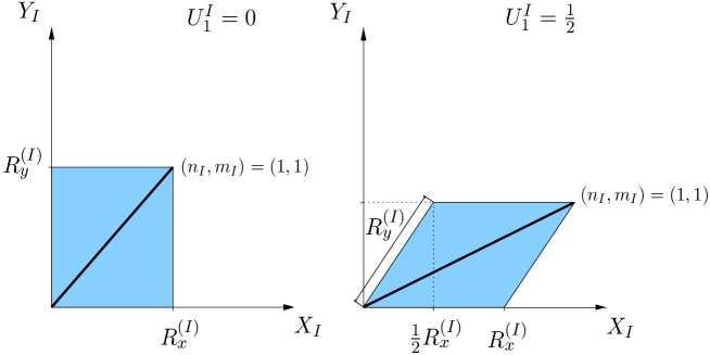
The action of the T-duality on the discrete $b$-flux is that the torus is either transformed into a rectangular one for $b_{I}=0$, or a tilted one for $b_{I}=1/2$. Commonly, the first possibility is called A-torus, the second possibility $B$-torus, both are shown in figure 2.2. As this choice can be taken differently for every 2-torus, in general this leads to eight distinct models.

The model is gauged under $\Omega R$, so under the worldsheet parity symmetry together with a spacetime and hence geometrical symmetry. To also hold within the presence of D-branes, this symmetry requires the introduction of an $\Omega R$-mirror brane for every D-brane.

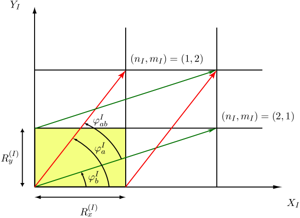
Furthermore, we make the assumption that the branes do not densely cover any one of the 2-tori. As a consequence, a set of two integers $(n_{I},m_{I})$ is sufficient to describe the position of any brane on the $I$-th 2-torus. $n_{I}$ and $m_{I}$ count the numbers by which the 1-cycle is wrapping the two fundamental cycles $\sqrt{1/2}R^{(I)}_{x}\mathbf{e}_{1}$, $m_{I}$ and $\sqrt{1/2}R^{(I)}_{y}\mathbf{e}_{2}$ of the torus, respectively. For uniqueness, one always has to choose the shortest length of any such brane representation, or more concretely, $n_{I}$ and $m_{I}$ always have to be coprime. Note, that by this definition, every brane has an orientation on the torus. The intersection angle (2.10) between two branes $D6_{a}$ and $D6_{b}$ then is given by

(2.11) $$\varphi^{I,\text{A}}_{ba}=\varphi^{I}_{b}-\varphi^{I}_{a}={\rm arctan}\left[\frac{\left(n_{I}^{a}m_{I}^{b}-m_{I}^{a}n_{I}^{b}\right)R^{(I)}_{x}R^{(I)}_{y}}{n_{I}^{a}n_{I}^{b}{R^{(I)}_{x}}^{2}+m_{I}^{a}m_{I}^{b}{R^{(I)}_{y}}^{2}}\right]$$

for the $A$-torus, or by

(2.12) $$\varphi^{I,\text{B}}_{ba}={\rm arctan}\left[{\frac{{R_{x}^{(I)}}\sqrt{4{{R_{y}^{(I)}}}^{2}-{{R_{x}^{(I)}}}^{2}}\left({n_{I}^{a}}{m_{I}^{b}}-{m_{I}^{a}}{n_{I}^{b}}\right)}{{{R_{x}^{(I)}}}^{2}{n_{I}^{a}}{m_{I}^{b}}+{{R_{x}^{(I)}}}^{2}{m_{I}^{a}}{n_{I}^{b}}+2{n_{I}^{a}}{{R_{x}^{(I)}}}^{2}{n_{I}^{b}}+2{m_{I}^{a}}{{R_{y}^{(I)}}}^{2}{m_{I}^{b}}}}\right]$$

for the B-torus. Both can be parameterized in one equation by

(2.13) $$\varphi^{I}_{ba}={\rm arctan}\left[{\frac{\frac{1}{2}{R_{x}^{(I)}}\sqrt{4{{R_{y}^{(I)}}}^{2}-2{b_{I}}{{R_{x}^{(I)}}}^{2}}\left({n_{I}^{a}}{m_{I}^{b}}-{m_{I}^{a}}{n_{I}^{b}}\right)}{{n_{I}^{a}}{n_{I}^{b}}{{R_{x}^{(I)}}}^{2}+{m_{I}^{a}}{m_{I}^{b}}{{R_{y}^{(I)}}}^{2}+{b_{I}}{{R_{x}^{(I)}}}^{2}\left({n_{I}^{a}}{m_{I}^{b}}+{m_{I}^{a}}{n_{I}^{b}}\right)}}\right]\ ,$$

for either $b_{I}=0$ or $b_{I}=1/2$ on a certain torus.

Another important observation is that one can define a topological intersection number $I_{ab}$ between two branes $a$ and $b$ by

(2.14) $$I_{ab}=\prod\limits_{I=1}^{3}\left(n_{I}^{a}m^{b}_{I}-m^{a}_{I}n^{b}_{I}\right)\ .$$

This number is topologically invariant and also has a very intuitive meaning. It gives the number of orientated intersections in between two branes, after all possible identified torus shifts of both branes along the two fundamental cycles of the torus have been regarded up to torus symmetries. A simple example is shown in figure 2.1, where the four differently orientated intersection numbers totally add up to three. Interestingly, this intersection number also can be derived just from the consistency requirement of the boundary state formalism with the CFT-loop channel calculations, as it is shown in appendix C.3.

2.1.3 Complex structure and Kähler moduli

The torus moduli $R^{(I)}_{x}$, $R^{(I)}_{y}$ and the angle $\theta$ between them can be mapped to different ones, the complex structure moduli $U^{I}$ and the Kähler structure moduli $T^{I}$. Loosely speaking, the imaginary part of $T^{I}$ is related to the volume of the torus and $U^{I}$ is related to the particular choice of the second lattice vector of the torus. For the case of D9-branes with $F$-fluxes, they can be defined in the following way:

(2.15) $\displaystyle U^{I}=U_{1}^{I}+iU_{2}^{I}=\frac{{R^{(I)}_{y}}}{{R^{(I)}_{x}}}\frac{\mathbf{e}_{2}}{\mathbf{e}_{1}}=\frac{R^{(I)}_{y}}{R^{(I)}_{x}}\ e^{i\theta}\ ,$
(2.16) $\displaystyle T^{I}=T^{I}_{1}+iT^{I}_{2}=b^{I}+iR^{(I)}_{x}R^{(I)}_{y}\sin\left(\theta\right)\ ,$

Note that in this equation, the discrete b-flux enters as well. The real part of $U^{I}$ can be chosen to be zero, corresponding to a rectangular torus with $\theta=\pi/2$. This actually is not a restriction on the model because $U_{1}^{I}$ is a continuous modulus of the theory.

Switching over to the T-dual description with $R^{\prime(I)}_{y}=1/R^{(I)}_{y}$, $T^{I}$ and $U^{I}$ are getting mapped into

(2.17) $\displaystyle T^{\prime I}=-\frac{1}{U^{I}}=-\frac{R^{(I)}_{x}}{R^{\prime(I)}_{y}}e^{-i\theta}\ ,$
$\displaystyle U^{\prime I}=-\frac{1}{T^{I}}=-\frac{b+i{R^{(I)}_{x}}{R^{\prime(I)}_{y}}\sin\left(\theta\right)}{b^{2}+{R^{(I)}_{x}}^{2}{R^{\prime(I)}_{y}}^{2}\sin^{2}\left(\theta\right)}\ .$

The torus now is tilted for the case $b=1/2\mod 1$, but there is no $B$-flux anymore. The significance of the tilt is that the projection of the second torus basis vector with a length ${R^{\prime(I)}_{y}}\sqrt{2}$ onto the $X_{I}$-axis is exactly $1/2$ of the length ${R^{\prime(I)}_{x}}\sqrt{2}$. Consequently, the angle $\theta$ between the torus vectors is fixed.

From now on, we will change the conventions on the branes at angles side. These are denoted in appendix D.1, together the two sets of basis vectors $\mathbf{e}_{i}^{\text{A}/\text{B}}$ for the two inequivalent torus possibilities, being depicted in figure 2.2. In common practice, these 2-tori are called A- and B-torus [39], here they are distinguished by the two values $b_{I}=0$ and $b_{I}=1/2$ from the flux picture. This notation will be kept, although there is no flux on the branes at angles side anymore.

Then, the complex structure and Kähler moduli take the following form

(2.18) $$U^{I}=b_{I}+i\sqrt{\frac{{R^{(I)}_{y}}^{2}}{{R^{(I)}_{x}}^{2}}-{b_{I}}^{2}}\ ,\qquad\qquad T^{I}=T_{1}^{I}+iR^{(I)}_{x}R^{(I)}_{y}\sqrt{1-{b_{I}}^{2}\frac{{R^{(I)}_{x}}^{2}}{{R^{(I)}_{y}}^{2}}}\ ,$$

where $b_{I}=0$ or $b_{I}=1/2$.

Refer to caption
Figure 2.2: The two inequivalent $A$- and $B$-tori, corresponding to $b=0$ and $b=1/2$ in the flux picture.

2.1.4 One-loop consistency

The partition function for the bosonic string (1.5) just contains the torus as a world-sheet at the one loop level, corresponding to an Euler number $\chi=0$. For our model, there are three additional worldsheets shown in figure 2.3 that all have this Euler number and so contribute at the same level.

Refer to caption
Figure 2.3: All four Riemann surfaces with $\chi=0$.

Two of them are unoriented, the Klein bottle and the Möbius strip, and two have boundaries, the cylinder (being conformally equivalent to an annulus) and again the Möbius strip. The two worldsheets with boundaries naturally are assigned to open strings ending on these boundaries, whereas the torus and the Klein bottle naturally are assigned to closed strings. The one-loop vacuum amplitude $\mathcal{Z_{\text{one-loop}}}$is the sum of all 4 contributions coming from the different $\chi=0$ worldsheets:

(2.19) $$\mathcal{Z_{\text{one-loop}}}=\mathcal{T}+\mathcal{K}+\mathcal{A}+\mathcal{M}\ .$$

Instead of the path integral representation of equation (1.5), it is also possible to work with the usual Hamiltonian formalism, where every worldsheet integral can be written as a trace, this is for instance for the cylinder amplitude up to normalization:

(2.20) $$\mathcal{A}\thicksim\int\limits_{0}^{\infty}\frac{dt}{t}\text{Tr}_{\text{open}}\left(\frac{1+(-1)^{F}}{2}e^{-2\pi t\mathcal{H}_{\text{open}}}\right)\ .$$

In this equation, $\mathcal{H}_{\text{open}}$ is the Hamilton operator for the open string and the projector within the trace is the usual GSO-projection, as discussed in the introductory chapter. The trace is taken over both Neveu-Schwarz and Ramond sectors and also includes the momentum integration $V_{10}/(2\pi)^{10}\int d^{10}p$, where $V_{10}$ is the regularized volume of a 10-torus. It is taken to be very large in order to obtain the theory in the flat 10-dimensional spacetime. $t$ is the modular parameter of the cylinder.

Taking a different point of view, the cylinder as a one-loop diagram for open strings can also be understood as a tree level propagation of a closed string. This is called open-closed string duality and schematically shown in figure 2.4.

Refer to caption
Figure 2.4: The open-closed string duality for the cylinder.

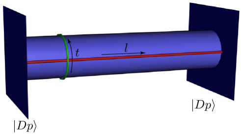
This duality can be understood via a modular transformation of the worldsheet’s modulus parameter $t$, schematically $t\rightarrow l\sim 1/t$. Usually the first point of view (2.19) is called loop channel, the second one tree-channel. The transformed amplitudes will be denoted by a tilde and can be written with boundary states:

(2.21) $$\widetilde{\mathcal{A}}\thicksim\int\limits_{0}^{\infty}dl\ \langle Dp|e^{-2\pi l\mathcal{H}_{\text{closed}}}|Dp\rangle\ .$$

The boundary states are coherent states in a generalized closed string Hilbert space, fulfilling the transformed boundary conditions which in the first place are being imposed on the open strings. In this picture, two specific boundary state objects have to be defined, $Dp$-branes and Orientifold $Op$-planes. Indeed, the loop channel amplitudes together with the boundary conditions are sufficient to completely specify the boundary states [72, 73]. We do not need their explicit form at this point.

For the torus and the Klein bottle, the modular transformation always transforms closed strings into closed strings, so the modular transformation then is not strictly an open-closed string duality for these worldsheets, but of course still possible to apply. In order to obtain the correct string lengths for the different amplitudes after the modular transformation, one has to take different normalizing factors into the definition of the tree channel modulus parameter $l$, this is summarized in table 2.2.

Topology Modular transformation
Cylinder(Annulus) $l=1/(2t)$
Klein bottle $l=1/(4t)$
Möbius strip $l=1/(8t)$
Table 2.2: The modular transformation parameters for the different topologies.

The torus amplitude $\mathcal{T}$ is modular invariant in type II string theory, and by this reason finite. This statement remains true for both our orientifold models, (2.1) and (2.8), because the torus amplitude stays unaltered. If the theory is supersymmetric in spacetime, then $\mathcal{T}$ by itself vanishes. This for instance is the case for type II string theory.

The three remaining worldsheets do not have the property of modular invariance, so for them it is not guaranteed that they do not contain any divergencies which generally can spoil the whole theory at the quantum level [74, 75]. These divergencies are called tadpoles in analogy to the field theory picture, where a single particle is generated from the vacuum by quantum effects. In string theory, a non-vanishing tadpole signals that the equations of motion of some massless fields in the effective theory are not satisfied. Regarding the different sectors of the superstring theory, both the R-R and the NS-NS sector of the closed superstring theory in the tree channel contribute to the overall tree channel tadpole. The two contributions, coming from these two sectors are usually called R-R and NS-NS tadpoles by themselves. One carefully has to distinguish the notion of R-R and NS-NS sectors for loop and tree channel, because the modular transformation maps one into the other, depending also on the spin structure. These maps are summarized for the different amplitudes without phase factors in table 2.3.

Amplitude Loop channel Tree channel
(NS-NS,$+$) (NS-NS,$+$)
Klein bottle (NS-NS,$-$) (R-R,$+$)
(R-R,$+$) (NS-NS,$-$)
(NS,$+$) (NS,$+$)
Cylinder (NS,$-$) (R,$+$)
(R,$+$) (NS,$-$)
(NS,$+$) (NS-NS,$-$)
Möbius strip (NS,$-$) (NS-NS,$+$)
(R,$+$) (R-R,$+$)
Table 2.3: Correspondence between different sectors in loop and tree channel.

Although the two tadpoles do appear on the same grounds in the partition function, their interpretation is quite different: $Dp$-branes as well as an orientifold $Op$-planes are p-dimensional hyperplanes of spacetime and therefore couple to R-R $(p+1)$-forms $A_{p+1}$, as was first pointed out in [25]. The orientifold plane by itself acts as a background charge (what we will see soon in the Klein bottle R-R contribution) which is a source term in the equations of motion for the field $A_{p+1}$:

(2.22) $$dH_{p+2}=\ast J_{7-p}\ ,\qquad d\ast{H_{p+2}}=\ast J_{p+1}\ .$$

Here, $J_{p+1}$ and $J_{7-p}$ are the electric and magnetic sources, respectively, and $H_{p+2}$ is the field strength of $A_{p+1}$. If the field equations shall be consistent, then the integral over the dual sources

(2.23) $$\int\limits_{\Sigma(\chi)}\ast J_{9-\chi}$$

for all surfaces $\Sigma(\chi)$ without boundaries has to vanish. This is nothing but the analogue to the simple Gauss law of electrodynamics. Using this picture, the field lines that are originated from one charge must either go to infinity or lead to another opposite charge. On a compact space, they cannot go to infinity and so must end on an opposite charge. If there is no such charge, the theory is inconsistent. This means for us that the orientifold $Op$-plane R-R charge has to be cancelled. There is just one possibility to do so, namely the introduction of open sting sectors and therefore $Dp$-branes that do exactly cancel the charge.333The argument first has been introduced for D9-branes in type IIB that are spacetime-filling. Here the restriction is even more severe: the 10-form potential does not have a field strength in a 10-dimensional spacetime. This fact implies that the R-R charges have to be neutralized locally, or in other words, the orientifold planes and D-branes have to lie on top of each other.

This indeed is possible in many cases and imposes severe restrictions on model building within orientifolds. Furthermore, non-vanishing R-R tadpoles are related to non-vanishing gauge anomalies in the effective field theory of the massless modes. These are certainly unacceptable.

On the other hand, the NS-NS tadpole seems to be not as bad as the R-R tadpole. The NS-NS sector contains the supergravity fields, in particular the dilaton and the graviton, and the dilaton-graviton interaction $\sqrt{-g}e^{-\Phi}$ is responsible for the tadpole that is often even called dilaton tadpole. The term appears as an overall factor in the effective action and having also a kinetic term which is absent for the R-R tadpole. The theory consequently is unstable (but not inconsistent). There are two different possibilities to treat this problem: In the first place, one can employ the Fischler-Susskind mechanism that already has been invented in the context of the bosonic string [76, 77]. The quantum corrections coming from the NS-NS tadpole induce a source term that gets incorporated into the equations of motion in this mechanism, leading to a space-dependent background value for the dilaton.

Secondly, there is the less ambitious approach: one might try to solve the string equations of motions including the dilaton tadpole in the effective field theory next to leading order. It has been demonstrated in [78, 79] that this generally leads to warped geometries and non-trivial profiles of the dilaton and other scalar fields. In the non-supersymmetric type I string theory discussed in these papers, the phenomenon of a spontaneous compactification has occurred due to the NS-NS tadpoles. This perhaps can be understood as a dynamical justification for a compactified spacetime. Sadly, the non-linear sigma model on the worldsheet then cannot be solved exactly in such a highly curved background and furthermore, the procedure does not lead to a vanishing tadpole at the next order of the perturbation theory. It merely is a hope that the non-supersymmetric string theory self-adjusts its background perturbatively order by order until eventually the true quantum vacuum with a vanishing tadpole to all orders is reached [80].

By way of contrast, if the string theory is supersymmetric in spacetime, then the sum of the two tadpoles vanishes for each world sheet topology separately because the corresponding trace is zero by supersymmetry and the NS-NS and R-R tadpoles are linked. On the other hand, this is not sufficient to guarantee the absence of divergencies, because it is just valid as long as no vertex operators have been inserted near one end of each worldsheet surface. Therefore, one demands that the two tadpoles are vanishing separately (or strictly speaking the one independent one has to be zero).

We will make these general remarks now more precise for the case of the $\Omega R$-orientifold containing D6-branes at angles. The R-R tadpoles first have been calculated for the $A$-torus in [81] and for the $B$-torus in the subsequent paper [59], the NS-NS tadpoles first have been treated in [64].

The orientifold plane is located at the fixed locus of the geometric action of $\Omega R$, so on the $X$-axis in figure 2.2. In the tree channel, the total amplitude $\widetilde{\mathcal{Z}}$ for one certain stack of $N$ D6-branes is given by the following equation:

(2.24) $$\widetilde{\mathcal{Z}}=\widetilde{\mathcal{K}}+\widetilde{\mathcal{A}}+\widetilde{\mathcal{M}}=\int\limits_{0}^{\infty}dl\ \Big{(}\langle D6|N+\langle O6|\Big{)}e^{-2\pi l\mathcal{H}_{\text{closed}}}\Big{(}|O6\rangle+N|D6\rangle\Big{)}\ ,$$

where $|D6\rangle$ and $|O6\rangle$ are the correctly normalized boundary states of the $N$ D6-branes and the one orientifold O6-plane. This sum of boundary states implies in the loop channel that the contributions of the different amplitudes factorize into a perfect square, what is schematically shown in figure 2.5, where a cross symbolically stands for a topological crosscap.

Refer to caption
Figure 2.5: Factorization of R-R and NS-NS tadpoles in the loop channel.

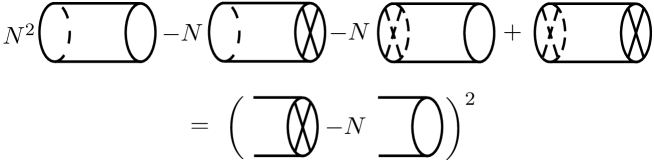
This factorization is very useful for actual computations, because it implies that it is sufficient to calculate for instance the Cylinder and Klein bottle amplitudes, and then use them to normalize the boundary states, after a transformation in the tree channel. By doing so, the Möbius strip amplitude is fixed unambiguously, without the need of an explicit calculation.

2.1.5 R-R tadpoles

Klein bottle

In order to find the correct normalization for the orientifold plane $|O6\rangle$, we will first calculate the R-R part of the Klein bottle tree channel amplitude which is given by

(2.25) $$\mathcal{K}^{\text{(NS-NS,$-$)}}=4c\int\limits_{0}^{\infty}\frac{dt}{t^{3}}\text{Tr}_{\text{(NS-NS,$-$)}}\left(\frac{\Omega R}{2}\ \frac{1+(-1)^{F}}{2}e^{-2\pi t\mathcal{H}_{\text{closed}}}\right),$$

in the loop channel, being reminded that (R-R,$+$) in the tree channel corresponds to (NS-NS,$-$) in the loop channel. The constant $c$ is given by $c=V_{4}/(8\pi^{2}\alpha^{\prime})^{2}$, where $V_{4}$ is the regularized volume of the 4-dimensional Minkowski spacetime. In order to evaluate the trace, one has to determine the Hamilton operator $\mathcal{H}_{\text{closed}}$, which in the loop channel NS-NS sector using (A.6) is just given by

(2.26) $${\mathcal{H}}^{\text{NS-NS}}_{\text{closed}}=({p^{\mu}})^{2}+\sum_{\mu}{\left(\sum_{n=1}^{\infty}{\left(\alpha_{-n}^{\mu}\alpha_{n}^{\mu}+\tilde{\alpha}_{-n}^{\mu}\tilde{\alpha}_{n}^{\mu}\right)}\right.}\\ \left.+\sum_{r\in\mathbb{Z}+1/2,\ r>0}{\left(r\psi^{\mu}_{-r}\psi^{\mu}_{r}+r\tilde{\psi}^{\mu}_{-r}\tilde{\psi}^{\mu}_{r}\right)}\right)+E_{0}^{\text{NS-NS}}+\mathcal{H}_{\text{lattice, cl.}}\ .$$

In order to obtain the zero point energy, we just have to correctly count the number of complex fermions and bosons in the sector and then use equation (A.9), from which we get:

(2.27) $$E_{0}^{\text{NS-NS}}=E_{0}^{\text{NS},L}+E_{0}^{\text{NS},R}=2\cdot 4\left(-\frac{1}{12}-\frac{1}{24}\right)=-1\ .$$

The lattice contribution can be found in appendix D.1. The trace over the oscillators and the zero-point energy can be treated separately from the lattice contribution, it just gives the standard NS-NS sector $\vartheta$-functions, so altogether

(2.28) $$\mathcal{K}^{\text{(NS-NS,$-$)}}=c\int\limits_{0}^{\infty}\frac{dt}{t^{3}}\frac{-\vartheta\bigg{[}{\begin{array}[]{*{20}c}0\\ 1/2\\ \end{array}}\bigg{]}^{4}}{\eta^{12}}\prod_{I=1}^{3}\left[\sum_{r_{I},s_{I}}e^{-\pi t\left(\frac{\alpha^{\prime}{s_{I}}^{2}}{{R_{x}^{(I)}}^{2}}\left(1+6b_{I}\right)+\frac{r_{I}^{2}}{\alpha^{\prime}}\left[\left(1+6b_{I}\right){R_{y}^{(I)}}^{2}-2b_{I}{R_{x}^{(I)}}^{2}\right]\right)}\right],$$

where $b_{I}$ can be chosen separately for every torus to be 00 or $1/2$, meaning an $A$- or $B$-torus, respectively. The argument of the $\vartheta$ and $\eta$-functions in this equation is $q=e^{-4\pi t}$. The amplitude can be transformed to the tree channel using $t=1/(4l)$, where equations (B.1), (B.2) and (B.4) have to be utilized. The result is given by:

(2.29) $$\widetilde{\mathcal{K}}^{\text{(R-R,$+$)}}=64c\int\limits_{0}^{\infty}{dl}\frac{\vartheta\bigg{[}{\begin{array}[]{*{20}c}1/2\\ 0\\ \end{array}}\bigg{]}^{4}}{\eta^{12}}\\ \prod_{I=1}^{3}\left[\frac{R_{x}^{(I)}}{\sqrt{1+6b_{I}}\sqrt{\left(1+6b_{I}\right){R_{y}^{(I)}}^{2}-2b_{I}{R_{x}^{(I)}}^{2}}}\sum_{r_{I},s_{I}}e^{-4\pi l\left(\frac{{s_{I}}^{2}{R_{x}^{(I)}}^{2}}{\alpha^{\prime}\left(1+6b_{I}\right)}+\frac{r_{I}^{2}\alpha^{\prime}}{\left(1+6b_{I}\right){R_{y}^{(I)}}^{2}-2b_{I}{R_{x}^{(I)}}^{2}}\right)}\right]\ .$$

Here, the $\vartheta$ and $\eta$-functions have the argument $q=e^{-4\pi l}$. The equation directly allows to determine the contribution of the Klein bottle to the tadpole, which will be denoted by $T$. It is just given by the zeroth order term in the $q$-expansion of the integrand in (2.29). Here, one has to use the explicit series or product expansions of the $\vartheta$ and $\eta$-functions (B.5) or (B.6) and (B.19). The result is given by

(2.30) $$T^{\text{R-R}}_{\widetilde{\mathcal{K}}}=1024c\prod_{I=1}^{3}\left[\frac{R_{x}^{(I)}}{\sqrt{1+6b_{I}}\sqrt{\left(1+6b_{I}\right){R_{y}^{(I)}}^{2}-2b_{I}{R_{x}^{(I)}}^{2}}}\right]\ .$$

and also allows to fix the normalization of the corresponding orientifold plane

(2.31) $$|O6\rangle=\mathcal{N}_{\text{O6}}\Big{(}|O6_{\text{NS}}\rangle+|O6_{\text{R}}\rangle\Big{)}\ ,$$

which is simply

(2.32) $$\mathcal{N}_{\text{O6}}=\frac{1}{2}\sqrt{{{T}^{\text{R-R}}_{\widetilde{\mathcal{K}}}}/16}\ .$$
Cylinder

Now we have to calculate the cylinder amplitude in the Ramond tree channel, where just (R,$+$) contributes, corresponding to the (NS,$-$) sector in the loop channel. For one stack of branes, the Cylinder amplitude contains 4 different contributions:

(2.33) $$\mathcal{A}=\mathcal{A}_{ii}+\mathcal{A}_{i^{\prime}i^{\prime}}+\mathcal{A}_{ii^{\prime}}+\mathcal{A}_{i^{\prime}i}\ .$$

The first term stands for the sector of open strings that stretch from a brane onto itself, the second one for the sector of strings that stretch from the $\Omega R$-mirror brane onto itself and the 3rd and 4th term for strings that stretch from the brane to its mirror brane and vice versa. The first two terms are easy to obtain, because there is no angle in between the two involved branes. The first one for the (NS,$-$) sector is given by

(2.34) $$\mathcal{A}_{ii}^{\text{(NS,$-$)}}=c\int\limits_{0}^{\infty}\frac{dt}{t^{3}}\text{Tr}_{\text{D6i-D6i}}^{\text{(NS,$-$)}}\left(\frac{1}{2}\frac{1+(-1)^{F}}{2}e^{-2\pi t\mathcal{H}_{\text{open}}}\right)\ .$$

The different normalization factor in front of the integral in comparison to (2.25) comes from the already performed momentum integration in the compact directions that is different for open and closed stings. The open string Hamiltonian is given by equation (A.8). Taking the trace over the oscillator modes and the zero mode, again leads to the standard NS-sector $\vartheta$- and $\eta$-functions, whereas the Kaluza-Klein and winding contributions can be determined using equation (D.18). This yields altogether for one stack of $N$ D-branes:

(2.35) $$\mathcal{A}_{ii}^{\text{(NS,$-$)}}=\frac{c}{4}N^{2}\int\limits_{0}^{\infty}\frac{dt}{t^{3}}\frac{-\vartheta\bigg{[}{\begin{array}[]{*{20}c}0\\ 1/2\\ \end{array}}\bigg{]}^{4}}{\eta^{12}}\prod_{I=1}^{3}\left[\sum_{r_{I},s_{I}}e^{-2\pi t\frac{r_{I}^{2}\left(1-b_{I}\right)+s_{I}^{2}\left[\left(1+2b_{I}\right){R_{x}^{(I)}}^{2}{R_{y}^{(I)}}^{2}-b_{I}{R_{x}^{(I)}}^{4}\right]}{\left(n_{I}^{2}+2b_{I}n_{I}m_{I}\right){R_{x}^{(I)}}^{2}+m_{I}^{2}{R_{y}^{(I)}}^{2}}}\right].$$

The argument of the $\vartheta$- and $\eta$-functions here is given by $q=e^{-2\pi t}$. The transformation to the tree channel by using $t=1/(2l)$ leads to the amplitude

(2.36) $$\widetilde{\mathcal{A}}_{ii}^{\text{(R,$+$)}}=\frac{c}{16}N^{2}\int\limits_{0}^{\infty}{dl}\frac{-\vartheta\bigg{[}{\begin{array}[]{*{20}c}1/2\\ 0\\ \end{array}}\bigg{]}^{4}}{\eta^{12}}\\ \prod_{I=1}^{3}\left[\frac{{\left(n_{I}^{2}+2b_{I}n_{I}m_{I}\right)\frac{R_{x}^{(I)}}{R_{y}^{(I)}}+m_{I}^{2}\frac{R_{y}^{(I)}}{R_{x}^{(I)}}}}{\sqrt{1-b_{I}}\sqrt{\left(1+2b_{I}\right)-b_{I}\frac{{R_{x}^{(I)}}^{2}}{{R_{y}^{(I)}}^{2}}}}\sum_{r_{I},s_{I}}e^{-\pi l\frac{\left(n_{I}^{2}+2b_{I}n_{I}m_{I}\right){R_{x}^{(I)}}^{2}+m_{I}^{2}{R_{y}^{(I)}}^{2}}{r_{I}^{2}\left(1-b_{I}\right)+s_{I}^{2}\left[\left(1+2b_{I}\right){R_{x}^{(I)}}^{2}{R_{y}^{(I)}}^{2}-b_{I}{R_{x}^{(I)}}^{4}\right]}}\right],$$

with an argument $q=e^{-4\pi l}$ of the $\vartheta$ and $\eta$-functions. The expansion in $q$ again leads to the tadpole:

(2.37) $$T^{\text{R}}_{\widetilde{\mathcal{A}}_{ii}}=-cN^{2}\prod_{I=1}^{3}\left[\frac{{\left(n_{I}^{2}+2b_{I}n_{I}m_{I}\right)\frac{R_{x}^{(I)}}{R_{y}^{(I)}}+m_{I}^{2}\frac{R_{y}^{(I)}}{R_{x}^{(I)}}}}{\sqrt{1-b_{I}}\sqrt{\left(1+2b_{I}\right)-b_{I}\frac{{R_{x}^{(I)}}^{2}}{{R_{y}^{(I)}}^{2}}}}\right]\ .$$

This is sufficient in order to determine the normalization of a general D6-brane as

(2.38) $$|D6\rangle=\mathcal{N}_{\text{D6}}\Big{(}|D6_{\text{i, NS}}\rangle+|D6_{\text{i, R}}\rangle\Big{)}\ ,$$

which is given by

(2.39) $$\mathcal{N}_{\text{D6}}=\frac{1}{2}\sqrt{{T^{\text{R}}_{\widetilde{\mathcal{A}}_{ii}}}/(16N^{2})}\ .$$

In general, there are two different possibilities how to further proceed. Either, one can determine the other sectors of the cylinder amplitude, which in general might get quite tedious, or one can calculate the Möbius amplitude, which is fixed by the two normalization factors, and then, by using the property of the perfect square, directly obtain the tadpole equations. This procedure indeed is sufficient, if all tadpoles receive contributions from the orientifold planes444This usuallly is the case for orbifold spaces that will be treated in the rest of the work., in the present case of the $\Omega R$-orientifold, some tadpoles are getting missed, and these are the ones that just come from the cylinder amplitude.

The mirror brane in terms of $n^{\prime}$ and $m^{\prime}$ is related to the original brane with wrapping numbers $n$ and $m$ by the map

(2.40) $\displaystyle n_{I}^{\prime}=n_{I}+2b_{I}m_{I}\ ,$
$\displaystyle m_{I}^{\prime}=-m_{I}\ .$

This simply means that to obtain the amplitude $\mathcal{A}_{i^{\prime}i^{\prime}}$, one just has to replace the $n_{I}$ and $m_{I}$ in the Kaluza-Klein and winding sum of (2.36) by $n_{I}^{\prime}$ and $m_{I}^{\prime}$, because the $\vartheta$-functions of the oscillator part, according to equation (A.8) just depend on the relative angle between the brane which is zero, as it was for $\mathcal{A}_{ii}$. On the other hand, the Kaluza-Klein and winding terms also remain unchanged after the map (2.40) has been applied, therefore $\mathcal{A}_{i^{\prime}i^{\prime}}=\mathcal{A}_{ii}$. The next amplitude which has to be calculated is $\mathcal{A}_{ii^{\prime}}$. This in general is much more difficult, because the two stacks of D-branes intersect at a non-vanishing angle. The general amplitude $\mathcal{A}_{ab}$ for any such angle is calculated in appendix C.3. For our present purpose, we have to insert the general winding numbers for the $a$-brane into the tree channel tadpole contribution (C.33) and for the $b$-brane the corresponding $\Omega R$-mirror wrapping numbers (2.40). Adding up all contributions (2.33), the overall cylinder tadpole is given by

(2.41) $$T^{\text{R}}_{\widetilde{\mathcal{A}}}=-16cN^{2}\left[\prod_{I=1}^{3}\left({\frac{\left({{n_{I}}}^{2}+2{b_{I}}{m_{I}}{n_{I}}\right){{R_{x}^{(I)}}}^{2}+{{m_{I}}}^{2}{{R_{y}^{(I)}}}^{2}}{\sqrt{4{{R_{y}^{(I)}}}^{2}-2{b_{I}}{{R_{x}^{(I)}}}^{2}}{R_{x}^{(I)}}}}\right)\right.\\ \left.+\prod_{I=1}^{3}\left({\frac{\left({{n_{I}}}^{2}+2{b_{I}}{m_{I}}{n_{I}}+2{{b_{I}}}^{2}{{m_{I}}}^{2}\right){{R_{x}^{(I)}}}^{2}-{{m_{I}}}^{2}{{R_{y}^{(I)}}}^{2}}{\sqrt{4{{R_{y}^{(I)}}}^{2}-2{b_{I}}{{R_{x}^{(I)}}}^{2}}{R_{x}^{(I)}}}}\right)\right]\ .$$

With the two contributions $T^{\text{R-R}}_{\widetilde{\mathcal{K}}}$ and $T^{\text{R}}_{\widetilde{\mathcal{A}}}$ at hand, we are able to write down the complete tadpole cancellation equation, which in our case is given by $T^{\text{R-R}}_{\widetilde{\mathcal{K}}}=T^{\text{R}}_{\widetilde{\mathcal{A}}}$, explicitly:

(2.42) $$-N^{2}\bigg{[}{{{m_{2}}}^{2}{{m_{1}}}^{2}\left({n_{3}}+{b_{3}}{m_{3}}\right)^{2}\frac{{R_{x}^{(3)}}{{R_{y}^{(1)}}}^{2}{{R_{y}^{(2)}}}^{2}}{{R_{x}^{(1)}}{R_{x}^{(2)}}}}\\ -{{}{{m_{1}}}^{2}{{m_{3}}}^{2}\left({n_{2}}+{b_{2}}{m_{2}}\right)^{2}\frac{R_{x}^{(2)}{{R_{y}^{(1)}}}^{2}{{R_{y}^{(3)}}}^{2}}{{R_{x}^{(1)}}{R_{x}^{(3)}}}}-{{{m_{2}}}^{2}{{m_{3}}}^{2}\left({n_{1}}+{b_{1}}{m_{1}}\right)^{2}\frac{{R_{x}^{(1)}}{{R_{y}^{(2)}}}^{2}{{R_{y}^{(3)}}}^{2}}{{R_{x}^{(2)}}{R_{x}^{(3)}}}}\\ +{{{m_{1}}}^{2}\big{(}{{b_{3}}}^{2}{{m_{3}}}^{2}\big{(}2{{b_{2}}}^{2}{{m_{2}}}^{2}+2{b_{2}}{m_{2}}{n_{2}}+{{n_{2}}}^{2}\big{)}+{{b_{2}}}^{2}{{m_{2}}}^{2}\big{(}2{b_{3}}{m_{3}}{n_{3}}+{{n_{3}}}^{2}\big{)}\big{)}\frac{{R_{x}^{(2)}}{R_{x}^{(3)}}{{R_{y}^{(1)}}}^{2}}{{R_{x}^{(1)}}}}\\ +{m_{2}}^{2}\big{(}{b_{1}}^{2}{m_{1}}^{2}\big{(}2{b_{3}}^{2}{m_{3}}^{2}+2{b_{3}}m_{3}n_{3}+{n_{3}}^{2}\big{)}+{b_{3}}^{2}{m_{3}}^{2}\big{(}2b_{1}m_{1}n_{1}+{n_{1}}^{2}\big{)}\big{)}\frac{{R_{x}^{(1)}}{R_{x}^{(3)}}{{R_{y}^{(2)}}}^{2}}{{R_{x}^{(2)}}}\\ +{{{m_{3}}}^{2}\big{(}{{b_{1}}}^{2}{{m_{1}}}^{2}\big{(}2{{b_{2}}}^{2}{{m_{2}}}^{2}+2{b_{2}}{m_{2}}{n_{2}}+{{n_{2}}}^{2}\big{)}+{{b_{2}}}^{2}{{m_{2}}}^{2}\big{(}2{b_{1}}{m_{1}}{n_{1}}+{{n_{1}}}^{2}\big{)}\big{)}\frac{{R_{x}^{(1)}}{R_{x}^{(2)}}{{R_{y}^{(3)}}}^{2}}{{R_{x}^{(3)}}}}\bigg{]}\\ -\bigg{[}\Big{(}{b_{1}}^{2}{m_{1}}^{2}\big{(}2{b_{2}}^{2}{m_{2}}^{2}+2b_{2}m_{2}n_{2}+{n_{2}}^{2}\big{)}\big{(}2{b_{3}}^{2}{m_{3}}^{2}+2b_{3}m_{3}n_{3}+{n_{3}}^{2}\big{)}+2n_{1}m_{1}b_{1}\\ \cdot\big{(}{n_{3}}^{2}\big{(}n_{2}+b_{2}m_{2}\big{)}^{2}+2n_{3}m_{3}b_{3}\big{(}n_{2}+b_{2}m_{2}\big{)}^{2}+{b_{3}}^{2}{m_{3}}^{2}\big{(}{n_{2}}^{2}+2{b_{2}}^{2}{m_{2}}^{2}+2b_{2}m_{2}n_{2}\big{)}\big{)}\\ +{n_{1}}^{2}\big{(}{n_{3}}^{2}\big{(}n_{2}+b_{2}m_{2}\big{)}^{2}+2m_{3}b_{3}n_{3}\big{(}n_{2}+b_{2}m_{2}\big{)}^{2}+{b_{3}}^{2}{m_{3}}^{2}\big{(}2{b_{2}}^{2}{m_{2}}^{2}+2b_{2}m_{2}n_{2}+{n_{2}}^{2}\big{)}\big{)}\Big{)}\\ -16\bigg{]}{R_{x}^{(1)}}{R_{x}^{(2)}}{R_{x}^{(3)}}=0\ .$$

In this equation, the products already have been evaluated and the resulting terms with different volume factors have been separated. Furthermore the substitution (C.35) has been applied. It is only possible to solve this tadpole cancellation equation in general, if all factors in front of the different volume factors vanish separately. This gives 7 different equations, but which are not all independent. Actually, the equations coming from the 4th, the 5th and the 6th term already are fulfilled if the first 3 equations are satisfied. By using these first 3 equations on equation 7, this equation can be drastically reduced and the final set of 4 tadpole equations is just given by

(2.43) $\displaystyle\sum_{i=1}^{k}{N_{i}}\prod_{I=1}^{3}\left({b_{I}^{i}}{m_{I}^{i}}+{n_{I}^{i}}\right)=16\ ,$
$\displaystyle\sum_{i=1}^{k}{N_{i}}{{m_{2}^{i}}}{{m_{3}^{i}}}\left({n_{1}^{i}}+{b_{1}^{i}}{m_{1}^{i}}\right)=0\ ,$
$\displaystyle\sum_{i=1}^{k}{N_{i}}{{m_{1}^{i}}}{{m_{3}^{i}}}\left({n_{2}^{i}}+{b_{2}^{i}}{m_{2}^{i}}\right)=0\ ,$
$\displaystyle\sum_{i=1}^{k}{N_{i}}{{m_{1}^{i}}}{{m_{2}^{i}}}\left({n_{3}^{i}}+{b_{3}^{i}}{m_{3}^{i}}\right)=0\ .$

This result here already has been generalized to the case of $k$ different stacks of D-branes, each consisting of $N_{i}$ parallel branes, and it is equivalent to the one in [57] for the A-torus and to the one in [59] for the B-torus. To see this, one has to transform the equations into the other chosen basis for the B-torus via $n^{\prime}_{I}\rightarrow n_{I}+b_{I}m_{I}$, $(m^{\prime}_{I}+b_{I}n^{\prime}_{I})\rightarrow m_{I}$ and also take into account the different definition for the second radius $R_{y}^{(I)\prime}\rightarrow\sqrt{{R_{y}^{(I)}}^{2}-{b_{I}}^{2}{R_{x}^{(I)}}^{2}}$, where the unprimed quantities are the ones of this work.

These tadpole equations also have a direct interpretation in the T-dual type I theory: the first equation in (2.43) demands the cancellation of the D9-brane and O9-plane charges against each other, the other three demanding a vanishing of the three possible types of D5-brane charges.

Connected to this, the R-R tadpole equations can even be understood by means of topology. They can be basis-independently written as

(2.44) $$\sum_{a=1}^{k}{N}_{a}\ \left(\pi_{a}+\pi^{\prime}_{a}\right)+Q_{q}\pi_{\rm Oq}=0\ ,$$

where $\pi_{a}$ denotes the homological cycle of the wrapped D$6_{a}$-branes and $\pi^{\prime}_{a}$ that of its $\Omega R$-mirrors. Furthermore, $\pi_{\rm Oq}$ denotes the cycle, the orientifold planes are wrapping on all three 2-tori. $Q_{q}$ is the charge of the orientifold plane that is fixed to be $Q_{6}=-4$ for four non-compact dimensions.

From this observation, it was possible to generalize intersecting brane model building to Calabi-Yau manifolds [82, 83]that do not have a simple description by conformal field theory, but still have known homology.

Möbius strip

In this chapter, we also write down the Möbius amplitude in the tree channel, which is far simpler to obtain than the cylinder amplitude. In particular, it will be needed for the $\mathbb{Z}_{N}$-orbifolds. The Möbius amplitude can be calculated directly from the overlap of a $|D6\rangle$ and a $|O6\rangle$ boundary state to be

(2.45) $$\widetilde{\mathcal{M}}_{[i]}^{\text{(R,$+$)}}=\pm N\int\limits_{0}^{\infty}{dl}\ 2\cdot 2\cdot 2\ \mathcal{N}_{\text{D6}}\ \mathcal{N}_{\text{O6}}\ \\ \cdot\gamma\ \frac{\vartheta\bigg{[}{\begin{array}[]{*{20}c}1/2\\ 0\\ \end{array}}\bigg{]}\vartheta\bigg{[}{\begin{array}[]{*{20}c}1/2\\ -\kappa_{1}\\ \end{array}}\bigg{]}\vartheta\bigg{[}{\begin{array}[]{*{20}c}1/2\\ -\kappa_{2}\\ \end{array}}\bigg{]}\vartheta\bigg{[}{\begin{array}[]{*{20}c}1/2\\ -\kappa_{3}\\ \end{array}}\bigg{]}}{\vartheta\bigg{[}{\begin{array}[]{*{20}c}1/2\\ 1/2-\kappa_{1}\\ \end{array}}\bigg{]}\vartheta\bigg{[}{\begin{array}[]{*{20}c}1/2\\ 1/2-\kappa_{2}\\ \end{array}}\bigg{]}\vartheta\bigg{[}{\begin{array}[]{*{20}c}1/2\\ 1/2-\kappa_{3}\\ \end{array}}\bigg{]}\eta^{3}}\ ,$$

where the argument of the modular functions is again given by $q=e^{-4\pi l}$. This amplitude needs some explanation: the three factors of 2 come from, firstly, the two possible spin structures, secondly, the two $\Omega R$-mirrors and finally, the interchangeability of the bra- and ket-vector. The bracket $[i]$ indicates that the Möbius amplitude is already taken over both branes contained in the equivalence class of the brane under consideration, the brane and its $\Omega R$-mirror.

Moreover, the product of the $\vartheta$-functions is formally equivalent to the one of the cylinder amplitude which has been derived in C.3, but the meaning of the moding is different, the angle $\varphi_{I}=\pi\kappa_{I}$ means the angle that the considered orientifold plane spans with the specific D-brane. Finally, the constant $\gamma$ has been introduced in order to cancel the contribution of the bosonic zero-modes by hand. After the expansion in $q$ and the use of the two simplifications (C.29), it turns out that $\gamma=2^{3}\prod_{I}\sin(\pi\kappa_{I})$ and the contribution from the modular functions in terms of the wrapping numbers together with $\gamma$ generally in lowest order is given by

(2.46) $$16\prod_{I=1}^{3}\cos(\pi\kappa_{I})=\\ 16\prod_{I=1}^{3}\frac{{R_{x}^{(I)}}^{2}\left(n_{I}^{\text{D}}n_{I}^{\text{O}}+b_{I}\left(n_{I}^{\text{D}}m_{I}^{\text{O}}+m_{I}^{\text{D}}n_{I}^{\text{O}}\right)\right)+{R_{y}^{(I)}}^{2}m_{I}^{\text{D}}m_{I}^{\text{O}}}{\sqrt{\left({n_{I}^{\text{D}}}^{2}+2b_{I}n_{I}^{\text{D}}m_{I}^{\text{D}}\right){R_{x}^{(I)}}^{2}+{m_{I}^{\text{D}}}^{2}{R_{y}^{(I)}}^{2}}\sqrt{\left({n_{I}^{\text{O}}}^{2}+2b_{I}n_{I}^{\text{O}}m_{I}^{\text{O}}\right){R_{x}^{(I)}}^{2}+{m_{I}^{\text{O}}}^{2}{R_{y}^{(I)}}^{2}}},$$

where the superscript D stands for the D-brane and O for the orientifold plane. This procedure assumes that the orientifold plane can be characterized by the 1-cycles it is wrapping on the torus, similarly to the D6-branes. In the present case, the wrapping numbers of the O6-plane are simply given by $n_{1}^{\text{O}}=n_{2}^{\text{O}}=n_{3}^{\text{O}}=1$ and $m_{1}^{\text{O}}=m_{2}^{\text{O}}=m_{3}^{\text{O}}=0$.

The resulting Möbius tadpole together with the Klein bottle tapole lead exacly to the same tadpole equation as the first one in (2.43), but does not reproduce the other three ones, as explained already.

2.1.6 NS-NS tadpoles

In the following, we are going to discuss the NS-NS tadpoles. These will be deduced in much less detail, because the methods are very similar. To keep the equations of manageable size, the case $b_{I}=0$ will be chosen during the computation, but the final result will be given for the general case.

Klein bottle

Starting again with the Klein bottle amplitude, we should first take a look at table 2.3. One observes that the two different spin structures of the tree channel NS-NS sector both contributing to the tadpole of interest, correspond to the two loop channels (NS-NS,$+$) and (R-R,$+$). Therefore, the only change as compared to (3.11) is that the theta function $-\vartheta[0,1/2]^{4}$ have to be replaced by the sum $\vartheta[0,0]^{4}-\vartheta[1/2,0]^{4}$, so

(2.47) $$\mathcal{K}^{\text{(NS-NS,$+$)}}+\mathcal{K}^{\text{(R-R,$+$)}}=c\int\limits_{0}^{\infty}\frac{dt}{t^{3}}\frac{\vartheta\bigg{[}{\begin{array}[]{*{20}c}0\\ 0\\ \end{array}}\bigg{]}^{4}-\vartheta\bigg{[}{\begin{array}[]{*{20}c}1/2\\ 0\\ \end{array}}\bigg{]}^{4}}{\eta^{12}}\prod_{I=1}^{3}\left[\sum_{r_{I},s_{I}}e^{-\pi t\left(\frac{\alpha^{\prime}{s_{I}}^{2}}{{R_{x}^{(I)}}^{2}}+\frac{r_{I}^{2}{R_{y}^{(I)}}^{2}}{\alpha^{\prime}}\right)}\right].$$

The straightforward computation leads to the tree channel tadpole:

(2.48) $$T^{\text{NS-NS}}_{\widetilde{\mathcal{K}}}=-1024{\frac{c{R_{x}^{(1)}}{R_{x}^{(2)}}{R_{x}^{(3)}}}{{R_{y}^{(1)}}{R_{y}^{(2)}}{R_{y}^{(3)}}}}\ .$$
Cylinder

Like for the R-R tadpole, the complete cylinder tree channel NS-tadpole for one stack of branes is a sum of the four contributions (2.33). The two contributions, where a string goes from one brane onto itself, $\widetilde{\mathcal{A}}_{ii}$ and $\widetilde{\mathcal{A}}_{i^{\prime}i^{\prime}}$, can be calculated like in section 2.1.5, if we again substitute the theta function coming from the fermions by the ones (NS,$+$) and (R,$+$), the Kaluza-Klein and winding sum remains unchanged. After the transformation into the tree channel and the expansion in $q$, the cylinder tadpole from $\widetilde{\mathcal{A}}_{ii}$ is given by

(2.49) $$T^{\text{NS}}_{\widetilde{\mathcal{A}}_{ii}}=T^{\text{NS}}_{\widetilde{\mathcal{A}}_{i^{\prime}i^{\prime}}}=-c{N}^{2}{\prod_{I=1}^{3}\frac{\left({{R_{x}^{(I)}}}^{2}{{n_{I}}}^{2}+{{R_{y}^{(I)}}}^{2}{{m_{I}}}^{2}\right)}{{R_{x}^{(I)}}{R_{y}^{(I)}}}}\ .$$

The general contribution with non-vanishing angle $\widetilde{A}_{ab}$ is more difficult to obtain, it is being calculated in appendix C.3.2. In our case, the two contributions $\widetilde{\mathcal{A}}_{ii^{\prime}}$ and $\widetilde{\mathcal{A}}_{i^{\prime}i}$ then directly can be written down from the general expression (C.44), if we proceed precisely as for the R-tadpole and in particular use the map (2.40) for the $\Omega R$-mirror brane. The final result for the cylinder NS-tadpole is given by:

(2.50) $$T^{\text{NS}}_{\widetilde{\mathcal{A}}}=-{\frac{c{N}^{2}}{\prod_{I=1}^{3}{R_{x}^{(I)}}{R_{y}^{(I)}}}}\left[{L_{1}}^{2}{L_{2}}^{2}{L_{3}}^{2}+\frac{{L_{2}}^{2}{L_{3}}^{2}}{{L_{1}}^{2}}\left({n_{1}}^{2}{R_{x}^{(1)}}^{2}-{m_{1}}^{2}{R_{y}^{(1)}}^{2}\right)\right.\\ \left.+\frac{{L_{1}}^{2}{L_{3}}^{2}}{{L_{2}}^{2}}\left({n_{2}}^{2}{R_{x}^{(2)}}^{2}-{m_{2}}^{2}{R_{y}^{(2)}}^{2}\right)+\frac{{L_{1}}^{2}{L_{2}}^{2}}{{L_{3}}^{2}}\left({n_{3}}^{2}{R_{x}^{(3)}}^{2}-{m_{3}}^{2}{R_{y}^{(3)}}^{2}\right)\right]\ ,$$

where

$$L_{I}=\sqrt{{n_{I}}^{2}{R_{x}^{(I)}}^{2}+{m_{I}}^{2}{R_{y}^{(I)}}^{2}}\ .$$

In this equation, $L_{I}$ is the length of the D-brane in consideration. Interestingly, the first term in the tadpole is different from the three others. We can understand this easily, if we are being reminded, of what are the massless fields in the NS-NS-sector in our model. In general, there is the four-dimensional dilaton and the 21 $\Omega{\cal R}$ invariant components of the internal metric and the internal NS-NS two form flux, but in our factorized ansatz with three 2-tori, only 9 moduli are evident. These are the six radions $R_{x}^{(I)}$ and $R_{y}^{(I)}$, which are related to the size of the internal dimensions and the two-form flux $b^{I}_{12}$ on each $T^{2}$. Consequently, we can already guess at this point that the first term in (2.50) is related to the dilaton, whereas the three other terms come from the radions.

From the cylinder tadpole together with the Klein bottle tadpole, we are now able to write down the full tadpole equations, using the property that the full tadpole is a sum of perfect squares. Naively, this seems to be problematic, because the volume factors in the Klein bottle tadpole seem to be different from the 4 contributions of the cylinder tadpole. On the other hand, thinking in terms of geometry, the location of the branes in the cylinder tadpole (2.50) comes up in terms of the winding numbers $n_{I}$ and $m_{I}$. The orientifold plane is located on the X-axis, so it has the winding numbers $n_{I}=1$ and $m_{I}=0$. If we insert this into the $L_{I}$ and the terms within the small brackets in the cylinder tadpole, we see that all terms indeed lead to the same volume factor. This also means, that we do have a second problem: we do not know, to which term the Klein bottle tadpole has to be assigned, such that the perfect square can be written down. The only way to answer this question is by calculating the Möbius amplitude, but the detailed calculation is being omitted at this point. The result is that the Klein bottle amplitude contributes equally to all four tadpoles. With this information, the tadpoles finally can be written down, starting with the dilaton tadpole and again allowing for both cases $b_{I}=0$ and $b_{I}=1/2$ and generalizing for $k$ stacks:

(2.51) $$\langle\phi\rangle_{D}={1\over\sqrt{{\rm Vol}(T^{6})}}\left(\sum_{a=1}^{k}N_{a}\,{\rm Vol}({\rm D}6_{a})-16\,{\rm Vol}({\rm O}6)\right)$$

with

(2.52) $${\rm Vol}({\rm D}6_{a})=\prod_{I=1}^{3}L_{I}({\rm D}6_{a})=\prod_{I=1}^{3}\sqrt{\left(\left(n_{I}^{a}\right)^{2}+2b_{I}n_{I}^{a}m_{I}^{a}\right){R_{x}^{(I)}}^{2}+\left(m_{I}^{a}{R_{y}^{(I)}}\right)^{2}}$$

and

(2.53) $${\rm Vol}({\rm O}6)=\prod_{I=1}^{3}L_{I}({\rm O}6)=\prod_{I=1}^{3}R_{x}^{(I)}\ .$$

The interpretation of this tadpole is simple, it just is a bookkeeping calculation of all volumes of both the D6-branes and the orientifold planes, the latter ones entering with a negative sign, as in the case of the R-tadpole. The dilaton tadpole is nothing else but the four-dimensional total tension in appropriate units. Interestingly, it is possible to express this tadpole entirely in terms of the imaginary part of the complex structure moduli $U_{2}^{I}$ of the three 2-tori:

(2.54) $$\langle\phi\rangle_{D}=\left(\sum_{a=1}^{k}N_{a}\,\prod_{I=1}^{3}\sqrt{\left(n_{I}^{a}+b_{I}m_{I}^{a}\right)^{2}\frac{1}{U_{2}^{I}}+\left(m_{I}^{a}\right)^{2}{U_{2}^{I}}}-16\,\prod_{I=1}^{3}\sqrt{\frac{1}{U_{2}^{I}}}\right).$$

We can understand this in realizing that the boundary and cross-cap states only couple to the left-right symmetric states of the closed string Hilbert space. The complex structure moduli are indeed left-right symmetric, whereas the Kähler moduli appear in the left-right asymmetric sector, i.e. D-branes and orientifold O6-planes only couple to the complex structure moduli. This is reversed in the T-dual type I picture, where the tadpole only depends on the Kähler moduli.

Now, we will discuss the remaining three radion tadpoles from (2.50), which in the language of complex structure and Kähler moduli correspond to tadpoles of the imaginary part of the tree complex structures:

(2.55) $$\langle U^{I}_{2}\rangle_{D}={1\over\sqrt{{\rm Vol}(T^{6})}}\left(\sum_{a=1}^{k}N_{a}\,v_{I}({\rm D}6_{a})\frac{L_{J}({\rm D}6_{a})\,L_{K}({\rm D}6_{a})}{L_{I}({\rm D}6_{a})}-16\,{\rm Vol}({\rm O}6)\right)\ ,$$

with $I\neq J\neq K\neq I$ and

(2.56) $$v_{I}({\rm D}6_{a})=\left(\left(n_{I}^{a}\right)^{2}+2b_{I}n_{I}^{a}m_{I}^{a}+2{\left(b_{I}m_{I}^{a}\right)}^{2}\right){R_{x}^{(I)}}^{2}-\left(m_{I}^{a}{R_{y}^{(I)}}\right)^{2}\ .$$

Also these tadpoles can be expressed entirely in terms of the imaginary part of the complex structure moduli, $U_{2}^{I}$. Concerning type II models which have been considered in similar constructions [84] , too, one needs to regard extra tadpoles for the real parts $U_{1}^{I}$, which cancel in type I. Looking more closely at the 4 NS-tadpoles, we realize that it is possible to express all of them as being derivatives from just one scalar potential in the string frame:

(2.57) $$V(\phi,U_{2}^{I})=e^{-\phi}\,\left(\sum_{a=1}^{k}N_{a}\,\prod_{I=1}^{3}\sqrt{\left(n_{I}^{a}+b_{I}m_{I}^{a}\right)^{2}\frac{1}{U_{2}^{I}}+\left(m_{I}^{a}\right)^{2}{U_{2}^{I}}}-16\,\prod_{I=1}^{3}\sqrt{\frac{1}{U_{2}^{I}}}\right)\ ,$$

meaning

(2.58) $$\langle\phi\rangle_{D}\sim{\partial V\over\partial\phi},\quad\quad\langle U^{I}_{2}\rangle_{D}\sim{\partial V\over\partial U^{I}_{2}}\ .$$

Comparing with the type II potential, the only change would be in erasing the term coming from the orientifold planes, and three more tadpoles would appear due to $\langle U_{1}^{I}\rangle_{D}\sim\partial V/\partial U_{1}^{I}$. As a side remark, although this potential is leading order in string perturbation theory, it already contains all higher orders in the complex structure moduli. So it is exact in these moduli, though we have only explicitly computed their one-point function, this fact needs a careful interpretation.

The term of the scalar potential coming from the D-branes also could have been anticipated from different considerations, as the source for the dilaton is just given by the tension of the branes, or to first order, by their volumes. The potential then arises by the Dirac-Born-Infeld action for a D9a-brane with a constant $U(1)$ and two-form flux

(2.59) $${\cal S}_{\rm DBI}=-\text{T}_{p}\int_{D9_{a}}{d^{10}x\ e^{-\phi}\sqrt{{\rm det}\left(G+(F_{a}+B)\right)}}\ ,$$

where $\text{T}_{p}$ stands for the Dp-brane tension

(2.60) $$\text{T}_{p}={\sqrt{\pi}\over 16\kappa_{0}}\left(4\pi^{2}\alpha^{\prime}\right)^{(11-p)/2}.$$

If we assume that all background fields are block-diagonal in terms of the two-dimensional tori, then they take the constant values [85]

(2.61) $\displaystyle G^{ij}=\delta^{ij},\quad\left(F_{a}^{I}\right)^{ij}={m_{a}^{I}\over n_{a}^{I}R_{x}^{I}\sqrt{{R_{y}^{(I)}}^{2}-{b_{I}}^{2}{R_{x}^{(I)}}^{2}}}\epsilon^{ij},$
$\displaystyle\left(B^{I}\right)^{ij}={b^{I}\over R_{x}^{I}\sqrt{{R_{y}^{(I)}}^{2}-{b_{I}}^{2}{R_{x}^{(I)}}^{2}}}\epsilon^{ij}\ .$

As a first step, one has to integrate out the internal six dimensions and take care of the fact that the brane wraps each torus $n_{I}^{a}$ times. Next, one only has to apply T-duality and then arrives at the same D-brane term of the derived potential.

We now come to the conclusions. As mentioned in the introduction already, a non-vanishing tadpole in perturbative field theory can be understood in such a way that the tree level value of the corresponding field has not been chosen at the minimum of the potential. Thus, even if higher loop corrections are formally computable, their meaning is very questionable, as fluctuations might be large, no matter how small the coupling constant actually is. As an resulting effect, the theory is driven away to a stable minimum, where now a meaningful perturbation theory is possible. Trying to apply this idea to our model, the only point where all four tadpoles vanish is at $U^{I}_{2}$=$\infty$. This is due to the R-R tadpole cancellation condition and the triangle inequality, and shows that a partial breaking of supersymmetry in ${\cal N}$=4 vacua by introducing relative angles between the D6-branes (or by the presence of magnetic fluxes on D9-branes) seems to be impossible, although such possibilities have been worked out in ${\cal N}$=2 type II and heterotic vacua [86, 87, 88, 89].

The potential displays a runaway behavior, which is quite typical for non-supersymmetric string models. The complex structure is dynamically pushed to its degenerate limit; all branes lie along the $X_{I}$ axes and the $Y_{I}$ directions shrink to zero,but still keeping the volume fixed. In other words, the positive tension of the branes pulls the tori towards the $X_{I}$-axes. The slope of the runaway behavior should be set by the tension proportional to the string scale, so we expect the system to decay quickly. The possibility that the potential shows a slow-roll behavior, as it is required by inflationary cosmological models will be discussed in chapter 5.

Furthermore, there is a second, related problem: if the $Y_{I}$ shrink to zero, and the angle between certain branes decreases, at some point open string tachyons, if not present already in the construction, dynamically appear and start to propagate at the open string tree level, this then indicates the decay of the brane configuration one has started with. Several aspects of this problem are discussed in some more detail in [90].

Our observation has strong consequences for all toroidal intersecting brane world models. These usually require a tuning of the parameters at tree-level and implicitly assume the global stability of the background geometry. But this geometry is determined by the closed string moduli, and if these display a runaway behavior, there is a contradiction. The instabilities translate back via T-duality into a dynamical decompactification towards the ten-dimensional supersymmetric vacuum.

To end this discussion, every non-supersymmetric toroidal model seems to be driven back to the degenerate supersymmetric vacuum. This also matches the observations of [91, 92, 93, 94] within the context of closed string tachyon condensation, where these problems are discussed using elaborate tools from quiver diagrams, RG-flows and the c-theorem.

2.2 Intersecting D6-branes on $\mathbb{Z}_{N}$-orientifolds

The models that we want to consider on the one hand shall be simple and completely solvable. On the other hand, they shall have the ingredients to break down supersymmetry in such a way that either $\mathcal{N}$=1 or even completely broken $\mathcal{N}$=0 supersymmetry in the effective 4-dimensional theory is possible.

To better understand this from string theory, one carefully has to distinguish in between the closed and open string sectors. In this section, we are interested in the closed string sector which does not notice the presence of D-branes. Therefore, the amount of conserved supersymmetry in this sector depends first on the specific model and a possible gauging (like $\Omega R$). Secondly, it has to be taken into account, how much of the remaining supercharges are conserved by the specific spacetime background.

Following [22], the classification of cyclic orbifold groups preserving $\mathcal{N}$=1 in 4 dimensions for the heterotic string is given in table 2.4. It is important to notice that this classification corresponds to a preservation of $\mathcal{N}$=2 in 4 dimensions in the case of type II models. For $\Omega R$-orientifolds, the number of supercharges of the closed string theory is reduced by half, so yielding $\mathcal{N}$=1 for the orbifolded models of the given table. Therefore, models of the type

(2.62) $${{\rm Type\ IIA}\ {\rm on}\ T^{6}\over\{G+\Omega RG\}}$$

will be discussed in the following chapters. The action for a discrete $G=\mathbb{Z}_{N}$ group can be explicitly given by

(2.63) $$Z^{L}_{I}\to e^{2\pi i{v_{I}}}\,Z^{L}_{I},\quad\quad Z^{R}_{I}\to e^{2\pi i{v_{I}}}\,Z^{R}_{I}\ .$$

These models are mapped under T-duality to asymmetric type I orbifolds where the Kähler moduli are frozen.

Orbifold group Action $(v_{1},v_{2},v_{3})$
$\mathbb{Z}_{3}$ $(1/3,\ \ 1/3,\ \ -2/3)$
$\mathbb{Z}_{4}$ $(1/4,\ \ 1/4,\ \ -1/2)$
$\mathbb{Z}_{6}$ $(1/6,\ \ 1/6,\ \ -1/3)$
$\mathbb{Z}_{6}^{\prime}$ $(1/6,\ \ 1/3,\ \ -1/2)$
$\mathbb{Z}_{7}$ $(1/7,\ \ 2/7,\ \ -3/7)$
$\mathbb{Z}_{8}$ $(1/8,\ \ 3/8,\ \ -1/2)$
$\mathbb{Z}_{8}^{\prime}$ $(1/8,\ \ 1/4,\ \ -3/8)$
$\mathbb{Z}_{12}$ $(1/12,\ 1/3,-5/12)$
$\mathbb{Z}_{12}^{\prime}$ $(1/12,\ 5/12,-1/2)$
Table 2.4: $\mathbb{Z}_{N}$-orbifold groups that preserve $\mathcal{N}$=2 in 4 dimensions for type II theory.

Looking at the classification table 2.4 in some more detail, it can be observed that the sum of the angles on the three 2-tori for all these orbifolds is zero. In the phenomenological model building of chapters 3 and 4, we will mainly concentrate on the first two entries of the table, the $\mathbb{Z}_{3}$ and $\mathbb{Z}_{4}$ groups, although an extension of the calculations to higher groups could resolve several emerging problems, but technically is even more difficult.

Orbifold constructions have not been first introduced in intersecting brane world scenarios with arbitrary angles. The orbifolding technique has already been used in some earlier papers, where D-branes have been introduced on top of the orientifold planes, see for instance [38, 39, 40, 95, 96, 97]. By doing so, the tadpoles have been cancelled locally. These models of course are generally supersymmetric.

2.2.1 R-R and NS-NS tadpoles

In order to determine the tadpoles of the model, one has to insert the additional projector

(2.64) $$\mathbf{P}=\frac{1+\Theta+\ldots+\Theta^{N-1}}{N}$$

into the trace of the four one-loop string amplitudes (2.19). This means for instance for the Klein-bottle amplitude [38, 40, 39]:

(2.65) $$\mathcal{K}=4c\int\limits_{0}^{\infty}\frac{dt}{t^{3}}\text{Tr}_{\text{U+T}}\left(\frac{\Omega R}{2}\ \frac{1+\Theta+\ldots+\Theta^{N-1}}{N}\ \frac{1+(-1)^{F}}{2}e^{-2\pi t\mathcal{H}_{\text{closed}}}\right),$$

where in general, both untwisted (U) and twisted (T) sectors have to be evaluated. In the tree channel, this can be understood in a simple manner: Generally, under both the $\mathbb{Z}_{N}$ and $\Omega R$ symmetry, the branes are organized in orbits of length $2N$. Such an orbit constitutes an equivalence class $[a]$ of D6a-branes and in the following will be denoted by $[(n_{I}^{a},m_{I}^{a})]$.

In order to determine the tadpoles in the untwisted sector, it is possible to proceed very close to the $\Omega R$ orientifold, with the important difference that we do not have to calculate the full cylinder amplitude (2.33), because all tadpoles receive a contribution from the orientifold plane and we can use the property of the perfect square and just need the normalization of the $\widetilde{A}_{ii}$ tree level amplitude. It would actually be very tedious to calculate the whole cylinder amplitude, as the orbit here has a length $2N$, not just a length two as for the $\Omega R$-orientifold.

Taking up the tree channel picture of orbits, it is very simple to generalize the calculation procedure of the two sections (2.1.5) and (2.1.6). Some important points have to be taken care of:

  1. 1.

    In general, there will not be only one orientifold plane anymore: in the discussed $\Omega R$-models, orientifold planes geometrically have been defined as being the fixed loci $\text{Fix}(R)|_{T^{6}}$ of the anti-holomorphic involution $R$ on the 6-torus. If the background space now is orbifolded, the whole orientifold group is generated by both $\Omega R$ and $\Theta$. Then the fixed locus on this quotient space also can be understood as being the orbit of the fixed locus on the torus in addition to the orbit of $\text{Fix}(\Theta R)|_{T^{6}}$, or more explicitly,

    (2.66) $$\text{Fix}(R)|_{\text{orbifold}}=\bigcup_{i=0}^{N-1}\Theta^{i}\left(\text{Fix}(R)|_{T^{6}}\right)\cup\Theta^{i}\left(\text{Fix}(\Theta R)|_{T^{6}}\right)\ .$$

    This is due to the relation

    (2.67) $$\Theta^{1/2}R\Theta^{-1/2}=\Theta R\ .$$

    There is an important subtlety that should be mentioned: only if $N\in 2\mathbb{Z}+1$, then $\Theta^{1/2}\in\mathbb{Z}$, and consequently, the two orbits in (2.66) are identical. Hence the $\mathbb{Z}_{3}$ and the $\mathbb{Z}_{4}$ models of the following chapters will include quite different features.

    Every one of the N terms $[\Theta^{i}\left(\text{Fix}(R)|_{T^{6}}\right)\cup\Theta^{i}\left(\text{Fix}(\Theta R)|_{T^{6}}\right)]$ can be treated as a separated orientifold plane and leads to a certain volume factor in the Klein bottle amplitude that in the end have to be summed up. Then, one can assign a normalization to every one of these $N$ orientifold planes, corresponding to a certain boundary state $|O6_{i}\rangle$. The Möbius amplitude in the tree channel can be obtained by the sum of $N$ distinct amplitudes of the form (3.23), where the normalization factor for the orientifold plane $\mathcal{N}_{\text{O6}_{i}}$ has to be substituted.

  2. 2.

    The Kaluza-Klein and winding contributions have to be calculated separately for every one of these $N$ orientifold planes, the reason lying in the fact that they have to respect different symmetries $\Omega R\Theta^{i}$ for $i=0,\ldots(N-1)$.

First, one has to calculate the tadpoles coming from the untwisted sector in the loop channel. If there are additionally contributions from the twisted sectors of the loop channel, a twist operator has to be inserted. This leads to theta functions with different characteristics $a$ in the loop channel, where $a$ simply is equivalent to the twist. The Kaluza-Klein and winding contributions might alter as well. Some other subtleties will be discussed for the specific example of the $\mathbb{Z}_{3}$- and $\mathbb{Z}_{4}$-orientifolds in the chapters 3.2, 3.3 and 4.4. The R-R tadpole often can be obtained more easily using the description in terms of homology, as can be seen for example for the $\mathbb{Z}_{4}$-orientifold in chapter 4.

2.3 Massless closed and open string spectra

In order to search for interesting phenomenological models, it is unavoidable to determine the low energy effective spectrum in four dimensions. The massive string excitations are organized in units of the string scale $\alpha^{\prime-1/2}$, so if we stick to the usual picture of a very high string scale, then the massive modes should be negligible at energies that today’s colliders might possibly achieve. From the string theoretical point of view, there are two different sectors that differ fundamentally, the open and closed string sectors. The closed string sector always includes the whole dimension of 10-dimensional spacetime, the so-called bulk, that in the picture of this work is factorized into a 4-dimensional flat Minkowski and a 6-dimensional compact space. It includes the supergravity multiplet and the dilaton, so it is fair to call it the gravitational sector. In contrast to this, the open string sector is determined by the specific D-brane content. In the modern understanding of string theory, they carry the gauge fields on their worldvolume (which in our case is 7-dimensional and always covers the whole Minkowski space) and just at the intersections on the compact space, there are chiral fermions [98], so the matter content of the standard model and its possible extensions. All these different sectors will be discussed now in more detail for the toroidal and orbifolded $\Omega R$-orientifolds.

2.3.1 Closed string spectrum

The closed string sector does not notice the presence of D-branes. Therefore, if one for now ignores the backreaction, the massless spectrum only depends on the chosen spacetime background and its moduli.

In order to find the massless states, one first has to compute the overall ground state energy in the sector of interest (that might be twisted as well) by the general formulae (A.9) for all bosons, NS- and R-sector fermions (with a general moding $\kappa$ corresponding to the twist).

In the untwisted sector, the left and right moving massless states that are $\Theta$-invariant have to be symmetrized and antisymmetrized under $\Omega R$ in both NS-NS and R-R sectors separately555This statement is valid for the purely toroidal $\Omega R$-orientifold as well, if one sets $\Theta=\text{Id}$.. Then the NS-NS sector always contributes the dilaton, the graviton and a certain number of neutral chiral multiplets.

In the twisted sector, the transformation properties of the fixed points, where the fields are localized, plays an important role: the fixed points that are separately invariant under $\Theta$ and $R$ are being treated as in the untwisted sector, they have to be symmetrized and antisymmetrized, too. The fixed points that are just invariant under a combination of $\Theta$ and $R$ require less symmetrization and the ones that are not invariant under $\Theta$ or $R$ no symmetrization at all. By this procedure, the total number of chiral plus vector multiplets turns out to be the sum of the two Hodge numbers $h_{1,1}+h_{2,1}$ , although the distribution between chiral and vector multiplets depends on the specific model, or in other words the choice of 2-tori. This is summed up for the models of interest in table 2.5.

Orbifold group Model Untwisted $\Theta+\Theta^{-1}$ twisted $\Theta^{2}\left(+\Theta^{-2}\right)$ twisted
$\mathbb{Z}_{3}$ AAA 9C+$g_{\mu\nu}$+$\Phi$ 14C+13V absent
$\mathbb{Z}_{3}$ AAB 9C+$g_{\mu\nu}$+$\Phi$ 15C+12V absent
$\mathbb{Z}_{3}$ ABB 9C+$g_{\mu\nu}$+$\Phi$ 18C+9V absent
$\mathbb{Z}_{3}$ BBB 9C+$g_{\mu\nu}$+$\Phi$ 27C absent
$\mathbb{Z}_{4}$ ABA 6C+$g_{\mu\nu}$+$\Phi$ 16C 15C+1V
$\mathbb{Z}_{4}$ ABB 6C+$g_{\mu\nu}$+$\Phi$ 12C+4V 15C+1V
Table 2.5: The d=4 closed string spectra for some $\mathbb{Z}_{N}$-orientifolds.

All of this is understandable in the context of general Calabi-Yau threefolds as well. There, the $\Omega R$-projection reduces the supersymmetry from $\mathcal{N}$=2 down to $\mathcal{N}$=1 and the bulk $\mathcal{N}$=2 superfields at the same time are truncated to $\mathcal{N}$=1 superfields. Before this truncation takes place there are $h_{1,1}$ abelian vector multiplets and $h_{2,1}$ hypermultiplets.

The $h_{1,1}$ vector multiplets consist of one scalar field coming from the dimensional reduction of the metric, the Kähler modulus $T$, and another scalar coming from the reduction of the NS-NS 2-form and a 4-dimensional vector from the reduction of the R-R 3-form along the 2-cycle on the specific torus. If the (1,1)-form is invariant under $\Omega R$, then a $\mathcal{N}$=1 chiral multiplet survives the projection. If instead it is anti-invariant, a $\mathcal{N}$=1 vector multiplet survives the projection.

The $h_{2,1}$ hypermultiplets consists of four scalar fields, where two are coming from the metric, the complex structure moduli $U$, and two arise from the dimensional reduction of the R-R 3-form along the two 3-cycles of $H^{2,1}(\mathcal{M})$ and $H^{1,2}(\mathcal{M})$. The $\Omega R$-projection now divides out one of two complex structure components and a linear combination of the R-R scalars survives this projection, such that the quaternionic complex structure moduli space is reduced to a complex moduli space of dimension $h_{2,1}$. It has to be like that because the $\mathbb{Z}_{N}$-orientifolds can be seen as singular limits of the corresponding Calabi-Yau space.

2.3.2 Open string chiral spectrum

The D6-branes carry the gauge fields via Chan-Paton factors at both ends of the open string. One has to distinguish in between branes that are not located along the fixed locus of the $\Omega R$-projection, so along the O6-planes, and the ones that are. One stack of the former ones supports a factor of $U(N_{a})$ to the total gauge group, a stack of the latter ones either an $SO(N_{a})$ or $Sp(N_{a})$ gauge factor [35]. Here, we will just be interested in the first more generic case, but still have to mention that in the T-dual case of D9 branes, the $U(N_{a})$ gauge group corresponds to a stack of D9 branes with non-vanishing flux, the $SO(N_{a})$ to a stack of D9 branes with vanishing flux, and the $Sp(N_{a})$ factor to stack of D5-branes that are allowed in the model as well [57].

For $k$ stacks of branes not on top of the O-planes, the total gauge group is given by

(2.68) $$\prod_{a=1}^{k}U(N_{a})\ ,$$

where these gauge groups are equipped with chiral matter in bifundamental, symmetric and antisymmetric representations that are located at the intersections on the compact space that break supersymmetry. It first has been clarified in [39] that the topological intersection number (2.14) on the torus or the orbifold space corresponds to the multiplicities of the certain representation, or in other words the number of fermion families. Thus this significant phenomenological model building property gets a completely geometric interpretation within the discussed orientifold models that arguably stays independent of continuous deformations of the moduli space.

Generally, there might be intersections between the two different types of branes, the branes and their $\Omega R$ mirror, each coming from the same stack or a different one. Furthermore, there are intersections with the orientifold plane. All these sectors give rise to different representations of the gauge group and it is important to mention that only the net intersection numbers on the torus or orbifold play a role for this chiral spectrum.

The sectors between two distinct stacks of branes generally lead to bifundamental representations. One has to distinguish between the intersection of a certain stack with another stack’s $\Omega R$ mirror, giving rise to chiral fermions in the bifundamental representation $(\overline{N}_{a},N_{b})$, and the sector between two distinct stacks where not both are $\Omega R$ mirrors within their stack. These sectors lead to $(N_{a},N_{b})$ representations. Formally negative intersection numbers, corresponding to flipped orientations on the torus or orbifold, simply enforce the conjugated representations.

However, there are also the intersections between branes within the same equivalence class. Open strings stretching between two $\Omega R$ mirrors, or for the case of the orbifold, between a brane and its $\Omega R\Theta^{k}$ mirror, lead to chiral fields in the antisymmetric and symmetric representation. Naively, there also could be intersections in between branes and their $\Theta$ mirrors that are no $\Omega R$ mirrors on the orbifold. These sectors would lead to matter in adjoint representations of the gauge group. However, in four flat dimensions they are absent, as the topological self-intersection numbers always vanish because of their antisymmetry for two 3-cycles. Still these sectors are part of the non-chiral spectrum.

This chiral spectrum can be expressed in terms of homological cycles too, and does not actually require a detailed CFT computation. It is shown for intersection numbers between these homological 3-cycles $\pi_{a}$ in table 2.6,

Representation Multiplicity
$[{\bf A_{a}}]_{L}$ ${1\over 2}\left(\pi^{\prime}_{a}\circ\pi_{a}+\pi_{{\rm O}6}\circ\pi_{a}\right)$
$[{\bf S_{a}}]_{L}$ ${1\over 2}\left(\pi^{\prime}_{a}\circ\pi_{a}-\pi_{{\rm O}6}\circ\pi_{a}\right)$
$[{\bf(\overline{N}_{a},N_{b})}]_{L}$ $\pi_{a}\circ\pi_{b}$
$[{\bf(N_{a},N_{b})}]_{L}$ $\pi^{\prime}_{a}\circ\pi_{b}$
Table 2.6: The massless chiral open string spectrum in 4 dimensions.

where the prime denotes $\Omega R$ mirror cycles,

(2.69) $$\pi_{a}^{\prime}\equiv\Omega R\pi_{a}\ ,$$

and $\pi_{{\rm O}6}$ the homological cycle of the O6-plane. Note, that for the case of the orbifold, one has to define the homological cycle on the orbifold space by

(2.70) $$\pi_{a}\equiv\sum_{i=0}^{N-1}\Theta^{i}\pi^{t}_{a}\ .$$

In this definition, the superscript $t$ denotes the toroidal ambient space. All intersection numbers have to be computed on the orbifold space, and the intersection between two 3-cycles then is given by [82]:

(2.71) $$\pi_{a}\circ\pi_{b}={1\over N}\left(\sum_{i=0}^{N-1}\Theta^{i}\pi^{t}_{a}\right)\circ\left(\sum_{j=0}^{N-1}\Theta^{j}\pi^{t}_{b}\right)\ .$$

In this language, it is immediately clear that there are no adjoint chiral representations in four dimensions, because $\pi_{a}\circ\pi_{a}=0$.

The spectrum of table 2.6 holds for more abstract general Calabi-Yau threefolds as well and in [82, 83] even a standard model on the Quintic has been constructed.

2.3.3 Open string non-chiral spectrum

The non-chiral open string spectrum can be obtained from the conformal field theory calculation at the orbifold limit of a more general Calabi-Yau space. In the language of boundary states, all the sectors between the stacks of branes, where the net topological intersection number is vanishing, give rise to non-chiral fields. It is possible but quite tedious to calculate this explicitly if one determines the open string partition function. To do so, the cylinder amplitude (3.18) has to be calculated (plus the Möbius amplitude) and the massless states directly can be read off.

First, for a certain stack of branes, there are the fields in the adjoint representation of the gauge group. They arise from the sectors in between a brane and its $\mathbb{Z}_{n}$ image, and are localized at this intersection point. In four compact dimensions these fields can be chiral, because the orbifold space intersection number $\pi_{a}\circ\pi_{a}$ can be non-vanishing. In six compact dimensions, the self-intersection $\pi_{a}\circ\pi_{a}$ due to its antisymmetry between two 3-cycles is always identically zero, therefore, the adjoint fermions are inevitably non-chiral.

Generally, there can be all fields from table 2.6 in the non-chiral spectrum if the net intersection number for a given representation is vanishing. For instance, for the bifundamental representations of the type $[{\bf(\overline{N}_{a},N_{b})}]_{L}$ in between two different stacks of branes, this definitely is the case if the branes are parallel on all tori.

The $U(1)$-factors have to be treated carefully in this respect. It is possible that they gain a mass through the Green-Schwarz-mechanism, as we will see in chapter 2.4.2, meaning that they drop out off the massless spectrum.

2.4 Anomalies

String theory claims to be a consistent theory of quantum gravity. Anomalies in simple terms indicate the breakdown of classical symmetries at the quantum level. One carefully has to distinguish in between anomalies in global and local symmetries. Anomalies in local symmetries lead to inconsistencies, and this is often linked to the breakdown of the renormalizability and unitarity of the theory. On the other hand, anomalies in global symmetries are unproblematic and just mean that the symmetry is no longer exact, this for instance is the case for the parity violation of the standard model.

Local gauge anomalies in four dimensions can be understood by one specific diagram, the famous Adler-Bell-Jackiw anomaly triangle,

Refer to caption
Figure 2.6: Non-abelian triangle anomaly diagram.

where a chiral fermion runs into a loop in between three external gauge bosons, see figure 2.6. No higher perturbative corrections occur. This statement has been proven by Adler and Bardeen and also has an extension to higher dimensional theories: in a $D$-dimensional theory, one just has to consider diagrams involving $D/2+1$ external gauge bosons. For 10-dimensional string theory, this means that one has to consider hexagon diagrams in spacetime. For intersecting brane models with six compact dimensions which are treated in this work, it is sufficient to use the effective massless spectrum in four dimensions and treat triangle diagrams, as this effective theory has to be consistent as well.

To understand spacetime anomalies from the viewpoint of string theory, one has to distinguish in between the closed and open string sectors of the theory.

The closed string sector basically is the sector of gravitational interactions. Before the emergence of string theory, there were consistent quantum field gauge theories, as for instance the most simple one, Quantumelectrodynamics, but it was not possible to construct a quantum field theory for gravity. So it was one of the most appreciated successes of string theory in its early days to show the absence of local gravitational anomalies [99], this indeed is the case for a total spacetime dimension $D=10$.

The open sector involves the specific content of D-branes and therefore, freedom from gauge anomalies has to be explicitly checked for any brane configuration. For the type I theory (or in other words, space-time filling D9-branes), anomaly freedom has been shown by Green and Schwarz in another ground-breaking work [74, 75]. For intersecting brane models, the freedom from gauge anomalies can be divided in two parts. First of all, there are the potential cubic anomalies, the non-abelian anomalies. Next, there are mixed anomalies involving the abelian symmetries. Finally, there are also mixed anomalies between the gravitational and the open string sectors.

As we already could have guessed, the freedom from gauge anomalies in the effective space-time theory is tightly connected to the consistence of the worlds-sheet formulation, or in other words to the R-R tadpole cancellation. If this tadpole is cancelled, the non-abelian anomalies automatically vanish, too. This result will be proven in the next section. In order to also see the cancellation of the mixed gauge anomalies and the mixed gravitational ones, one has to use the Green-Schwarz mechanism, this will be treated in section 2.4.2.

2.4.1 Non-abelian anomalies

The non-abelian gauge anomalies can be calculated in a simple manner. One has to convert all occurring trace contributions of the type that can be seen in figure 2.6 into traces over field strengths in the fundamental representation of the gauge group, $\text{Tr}_{\text{N}}F^{3}$. For the possible representations, this is shown in table 2.7.

$\text{Tr}_{\text{S}}F^{3}$ $\left(N+4\right)\text{Tr}_{\text{N}}F^{3}$
$\text{Tr}_{\text{A}}F^{3}$ $\left(N-4\right)\text{Tr}_{\text{N}}F^{3}$
$\text{Tr}_{\bar{\text{N}}}F^{3}$ $-\text{Tr}_{\text{N}}F^{3}$
Table 2.7: Conversion of cubic traces in different representations (left) into traces of the fundamental representation (right) of the gauge group $U(N)$, $N>1$.

With this information at hand, we can simply take the sum over all contributions of the chiral spectrum from table 2.6, this explicitly reads for $k$ stacks

(2.72) $\displaystyle A_{\text{non-abelian}}=$ $\displaystyle\sum_{a=1}^{k}\bigg{[}\left(\frac{N_{a}}{2}+2\right)\left(\pi^{\prime}_{a}\circ\pi_{a}-\pi_{{\rm O}6}\circ\pi_{a}\right)$
$\displaystyle+\left(\frac{N_{a}}{2}-2\right)\left(\pi^{\prime}_{a}\circ\pi_{a}+\pi_{{\rm O}6}\circ\pi_{a}\right)\bigg{]}$
$\displaystyle=$ $\displaystyle\sum_{a=1}^{k}\Big{[}N_{a}\left(\pi_{a}+\pi^{\prime}_{a}\right)-4\pi_{{\rm O}6}\Big{]}\circ\pi_{a}-\sum_{a=1}^{k}N_{a}\pi_{a}\circ\pi_{a}$
$\displaystyle=$ $\displaystyle-\sum_{a=1}^{k}N_{a}\pi_{a}\circ\pi_{a}=0\ ,$

where we have used the R-R tadpole cancellation condition (2.44) and the fact that $\pi_{a}\circ\pi_{a}=0$. Indeed, the non-abelian gauge anomaly ${SU(N_{a})}^{3}$ generally vanishes.

2.4.2 Generalized Green-Schwarz mechanism

In this section, we will discuss the mixed anomalies of the type $U(1)_{a}-SU(N_{b})^{2}$. These anomalies can be calculated again from the chiral spectrum in table 2.6 for the effective 4-dimensional theory, where we have to use different conversions for the traces, given in table 2.8.

$\text{Tr}_{\text{S}}F^{2}$ $\left(N+2\right)\text{Tr}_{\text{N}}F^{2}$
$\text{Tr}_{\text{A}}F^{2}$ $\left(N-2\right)\text{Tr}_{\text{N}}F^{2}$
$\text{Tr}_{\text{adj}}F^{2}$ $2\,N\,\text{Tr}_{\text{N}}F^{2}$
$\text{Tr}_{\bar{\text{N}}}F^{2}$ $\text{Tr}_{\text{N}}F^{2}$
Table 2.8: Conversion of quadratic traces in different representations (left) into traces of the fundamental representation (right) of the gauge group $U(N)$, $N>1$.

The result for $a\neq b$, where just the bifundamentals contribute, is given by

(2.73) $$A_{\text{mixed}}^{\text{$1^{\text{st}}$part}}=\frac{N_{a}}{2}\left(\pi^{\prime}_{a}-\pi_{a}\right)\circ\pi_{b}\ \qquad\text{for}\ {a\neq b}\ .$$

On the other hand for $a=b$, the anomaly is given by

(2.74) $\displaystyle A_{\text{mixed}}^{\text{$1^{\text{st}}$part}}=$ $\displaystyle-2\,\pi_{{\rm O}6}\circ\pi_{a}+N_{a}\,\left(\pi^{\prime}_{a}\circ\pi_{a}\right)$
$\displaystyle-\frac{1}{2}\sum_{b\neq a}N_{b}\pi_{a}\circ\left(\pi_{b}+\pi^{\prime}_{b}\right)\ \qquad\text{for}\ {a=b}\ .$

This equation can be reduced to the form (2.73) by the use of the tadpole equation (2.44). This anomaly at first sight seems to be existing. It was a very important result by Green and Schwarz, who were discussing the type I string, that by a careful study after all a term indeed can be identified cancelling this formal anomaly [74, 75]. The general idea is that besides the metric and the gauge fields, in string theory there are also Chern-Simons interactions, being invariant under gauge transformations of the vector potential because of their construction from the field strength.

Here, we implement a generalized Green-Schwarz mechanism analogously to [84] to chancel the anomaly (2.73). The Chern-Simons terms to be considered are of the form

(2.75) $$\int_{D6_{a}}C_{3}\wedge\text{Tr}\left(F_{a}\wedge F_{a}\right)\qquad\text{and}\qquad\int_{D6_{a}}C_{5}\wedge\text{Tr}\left(F_{a}\right)\ .$$

In this equation, $C_{3}$ is the antisymmetric 3-form and $C_{5}$ the 10-dimensional Hodge dual 5-form and $F_{a}$ denotes the gauge field strength on the $D6_{a}$-brane. To further proceed, we have to define a homological basis $e_{I}$, where $I=0,\ldots,h_{2,1}$ and its dual basis $e_{I}^{\ast}$, such that

(2.76) $$e_{I}\,e_{J}^{\ast}=\delta_{IJ}\ .$$

Any 3-cycle (also fractional 3-cycles) and its mirror $\pi^{\prime}_{a}$ now can be expanded in the basis $(e_{I},e_{I}^{\ast})$,

(2.77) $\displaystyle\pi_{a}=v_{a}^{I}\,e_{I}+v_{a}^{(I+h_{2,1}+1)}\,e_{I}^{\ast}\ ,$
$\displaystyle\pi^{\prime}_{a}=v_{a}^{I\prime}\,e_{I}+v_{a}^{(I+h_{2,1}+1)\prime}\,e_{I}^{\ast}\ .$

One furthermore has to define the 4-dimensional axions $\Phi_{I}$ and 2-forms $B_{I}$, such that

(2.78) $\displaystyle\Phi_{I}=\int_{e_{I}}C_{3}\ ,$ $\displaystyle\Phi_{I+h_{2,1}+1}=\int_{e_{I}^{\ast}}C_{3}\ ,$
$\displaystyle B_{I}=\int_{e_{I}^{\ast}}C_{5}\ ,$ $\displaystyle B_{I+h_{2,1}+1}=\int_{e_{I}}C_{5}\ .$

Then, the Chern-Simons couplings (2.75) can be rewritten as

(2.79) $\displaystyle\int_{D6_{a}}C_{3}\wedge\text{Tr}\left(F_{a}\wedge F_{a}\right)=\sum_{J=0}^{2h_{2,1}}\left(v_{a}^{J}+v_{a}^{J\prime}\right)\int_{\mathbb{R}^{1,3}}\Phi_{I}\wedge\text{Tr}\left(F_{a}\wedge F_{a}\right)\ ,$
$\displaystyle\int_{D6_{a}}C_{5}\wedge\text{Tr}\left(F_{a}\right)=N_{a}\sum_{I=0}^{h_{2,1}}\left(v_{a}^{(I+h_{2,1}+1)}-v_{a}^{(I+h_{2,1}+1)\prime}\right)\int_{\mathbb{R}^{1,3}}B_{I}\wedge F_{a}$
$\displaystyle\qquad\qquad\qquad\qquad+N_{a}\sum_{J=0}^{h_{2,1}}\left(v_{a}^{J}-v_{a}^{J\prime}\right)\int_{\mathbb{R}^{1,3}}B_{J+h_{2,1}+1}\wedge F_{a}\ ,$

where it has been used that the gauge field on the $\Omega R$-mirror brane is equivalent to $F_{a}^{\prime}=-F_{a}$. The prefactor $N_{a}$ arises from the normalization of the $U(1)$-generator.

From these two couplings, one gets a contribution to the discussed mixed anomaly between the $U(1)$ gauge factor from the first stack of branes and its coupling to $B$ and the two $SU(N)$ gauge factors and their coupling to $\Phi$. This is schematically shown in figure 2.7.
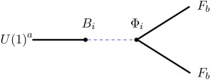
Refer to caption
Figure 2.7: The generalized Green-Schwarz mechanism.

This simply means that the $i$-th twisted field first couples to the $U(1)^{a}$, then propagates and finally couples to $F_{b}^{2}$. Therefore, the total anomaly contribution is given by

(2.80) $\displaystyle A_{\text{mixed}}^{\text{$2^{\text{nd}}$part}}$ $\displaystyle\sim N_{a}\sum_{I=0}^{h_{2,1}}\Bigg{[}\left(v_{a}^{I}+v_{a}^{I\prime}\right)\left(v_{b}^{(I+h_{2,1}+1)}-v_{b}^{(I+h_{2,1}+1)\prime}\right)$
$\displaystyle\qquad\qquad\qquad\qquad\qquad\qquad+\left(v_{a}^{(I+h_{2,1}+1)}+v_{a}^{(I+h_{2,1}+1)\prime}\right)\left(v_{a}^{I}-v_{a}^{I\prime}\right)\Bigg{]}$
$\displaystyle=2\,N_{a}\left(\pi_{a}-\pi^{\prime}_{a}\right)\circ\pi_{b}\ \qquad\text{for}\ {a\neq b}\ .$

This term has the right form to cancel the anomaly (2.73).

The kernel of the matrix $M_{aI}$, which can be defined by

(2.81) $$M_{aI}=N_{a}(v_{a}^{I}-v_{a}^{I\prime})\ ,$$

yields the non-anomalous $U(1)$ gauge groups of the specific model, which remain massless after the application of the Green-Schwarz mechanism.

2.5 Gauge breaking mechanisms

In this section several possible gauge breaking mechanisms will be discussed in the context of intersecting D-brane configurations. This is a very vivid topic, so we can just give a glimpse of the different possibilities. Some more information can be found in [59, 64, 48, 66, 67, 61, 100, 101, 102].

2.5.1 Adjoint higgsing

The simplest possibility for gauge symmetry breaking is to separate a stack of $N_{a}$ D-branes into two stacks, containing $N_{b}$ and $N_{c}$ D-branes, where $b+c=a$. This breaks the gauge groups from $U(N_{a})$ down to $U(N_{b})\times U(N_{c})$ and corresponds to giving a VEV to the respective fields in the adjoint representation of the gauge group $U(N_{a})$. The intersection numbers on the torus remain unchanged by this operation. Of course, the Green-Schwarz mechanism has to be performed again after this gauge symmetry breaking.

2.5.2 Brane recombination mechanisms

The mechanism of adjoint higgsing certainly leaves the branes flat and factorizable, so one still has a description by conformal field theory. On the other hand, string theory also allows for processes which are not of this type. A D-brane can be deformed but still homologically wrap the same 3-cycles on the underlying Calabi-Yau manifold. Unfortunately, the CFT description on the orbifold point then does not apply anymore. To understand this process, one has to distinguish in between sectors that preserve $\mathcal{N}$=2 and those that just preserve $\mathcal{N}$=1 supersymmetry.

Sectors preserving $\mathcal{N}$=2 supersymmetry

The mechanism being described in this first section can also be understood as a Higgs mechanism in low energy field theory, although its string theoretical realization is different to the one of the preceding section. Again, one gives VEV to some of the open string massless fields and leaves the closed string background unchanged.

This mechanism in our class of models is possible if two stacks of D-branes preserve a common ${\cal N}=2$ supersymmetry, meaning that they have to be parallel on one of the three 2-tori. In this case, there exists a massless hypermultiplet, $H$, being localized on the intersection of these two branes. $H$ then signals a possible deformation of the two stacks of D-branes into recombined D-branes, this can be seen for a specific example in figure 4.3. These still wrap complex cycles and have the same volume as the sum of volumes of the two D-branes before the recombination process occurs. There exists a flat direction $\langle h_{1}\rangle=\langle h_{2}\rangle$ in the D-term potential

(2.82) $$V_{D}={1\over 2g^{2}}\left(h_{1}\bar{h}_{1}-h_{2}\bar{h}_{2}\right)^{2}\ ,$$

along which the $U(N)\times U(N)$ gauge symmetry is broken to the diagonal subgroup $U(N)$, but supersymmetry remains unbroken.666This is not possible for the special case that on one of the two stacks there only sits a single D6-brane: then the F-term potential $\phi h_{1}h_{2}$ forbids the existence of a flat direction with $\langle h_{1}\rangle=\langle h_{2}\rangle$. In string theory, the explanation for this fact is that there do not exist large instantons in the $U(1)$ gauge group. In this equation, $h_{1}$ and $h_{2}$ denote the two complex bosons inside of one hypermultiplet. So there exists an open string massless field acting like a low energy Higgs field. In the T-dual picture, this process is nothing but the deformation of a small instanton into an instanton of finite size. In intersecting brane orientifold models, such ${\cal N}=2$ Higgs sectors are coupled at brane intersections to chiral ${\cal N}=1$ sectors. One still has to be careful, because the brane recombination in the effective gauge theory cannot simply be described by the renormalizable couplings. In order to get the correct light spectrum, one also has to take into account higher dimensional couplings from string theory, that might alter the qualitative picture.

This process is also possible if the two stacks of branes $U(N_{a})$ and $U(N_{b})$ have a different number of branes $N_{a}\neq N_{b}$. Then, a gauge breaking of the following kind might occur:

(2.83) $$U(N_{a})\times U(N_{b})\rightarrow U\left(\text{min}\{N_{a},N_{b}\}\right)\times U\left(\text{max}\{N_{a},N_{b}\}-\text{min}\{N_{a},N_{b}\}\right)\ ,$$

where equally many branes from the one and the other stack recombine and the rest stays unaltered.

Sectors preserving $\mathcal{N}$=1 supersymmetry

The situation is different for the case that two D-branes only preserve a common ${\cal N}=1$ supersymmetry and support a massless chiral supermultiplet $\Phi$ on the intersection [103, 104, 105]. In this case, the analogous D-term potential to (2.82) schematically is of the following form

(2.84) $$V_{D}={1\over 2g^{2}}\left(\phi\bar{\phi}\right)^{2}\ .$$

It is not possible to obtain a flat direction in this potential by just giving a VEV to the massless boson $\phi$, if there are no other chiral fields involved in the process.

Nevertheless, the massless fields still indicate for isolated brane intersections that the complex structure moduli are chosen on a line of marginal stability. If one moves away from this line in one direction, the intersecting branes will break supersymmetry without the appearance of a closed string tachyon, indicating that the intersecting brane configuration is stable. But if one moves away from the line in the other direction, the former massless chiral fields will become tachyonic.

The question now arises if it is possible to find another new supersymmetric ground state of the system on the line of marginal stability, where some of the original gauge symmetries are broken, in general involving non-flat D-branes that nevertheless wrap special Lagrangian 3-cycles.

On the compact 6-torus, bifundamental chiral multiplets do at least locally indicate the existence of a recombined brane, having the same volume but broken gauge groups. Gauge breaking now is possible if only certain bifundamental fields between different stacks of branes would become tachyonic under an enforced continuous complex structure deformation. If at the same time, one gives a VEV to these fields, this actually does not happen, but the system stays on the line of marginal stability. Nevertheless, the gauge groups of the potentially tachyonic fields are broken for the new system with the recombined branes.

We will make this discussion now more precise: from general arguments for open string models with ${\cal N}=1$ supersymmetry, it is known that the complex structure moduli only appear in the D-term potential, whereas the Kähler moduli only appear in the F-term potential [106, 107, 108, 109], the sum of which yielding the total scalar potential for the field $\phi$.

Therefore, one has to shown that the D-terms allow for a flat direction in the potential. A small variation of the complex structure on the field theory side corresponds to including a Fayet-Iliopoulos term $r$ into the D-term potential

(2.85) $$V_{D}={1\over 2g^{2}}\left(\phi\bar{\phi}+r\right)^{2}\ .$$

To see the precise form of $r$, we take another look at the Chern-Simons couplings of the D-brane effective action (2.79) which has the form of an $F$-term. The corresponding D-term involves a coupling of the auxiliary field $D_{a}$

(2.86) $$S_{\text{FI}}=\sum_{i=1}^{b_{3}}\sum_{a=1}^{k}\int d^{4}x\,M_{ai}\,{\partial{\cal K}\over\partial\phi_{i}}\,{1\over N_{a}}\,{\rm tr}(D_{a})\ .$$

where the $\phi_{i}$ are the superpartners of the Hodge duals of the RR 2-forms. ${\cal K}$ denotes the Kähler potential.

These couplings give rise to Fayet-Iliopoulos terms depending on the complex structure moduli which we simply parameterize by $A_{i}={\partial{\cal K}/\partial\phi_{i}}$. We do not need the precise form of the Kähler potential as long as the map from the complex structure moduli $\phi_{i}$ to the new parameters $A_{i}$ is one to one. This indeed is the case due to the positive definiteness of the metric on the complex structure moduli space. The D-term potential including only the chiral matter and the FI-terms in general reads

(2.87) $\displaystyle V_{\text{D}}$ $\displaystyle=\sum_{a=1}^{k}\sum_{r,s=1}^{N_{a}}{1\over 2g_{a}^{2}}(D^{rs}_{a})^{2}\ ,$

where the indices $(r,s)$ numerate the $N_{a}^{2}$ gauge fields in the adjoint representation of the gauge factor $U(N_{a})$. For a specific configuration, after inserting the $U(1)$ charges $q_{ai}$ and the Green-Schwarz couplings $M_{ai}$, one now has to find specific complex structure deformations $A_{i}$ which just alter some of the 3-cycles. The branes (and consequently the bifundamental fields) wrapping these specific cycles are getting deformed, the bifundamental fields would then become tachyonic and to prevent this, one gives a VEV to these fields. Consequently, they drop out of the massless spectrum and on the side of string theory, the involved branes have recombined into a new in general non-factorizable one, which still wraps a special Lagrangian 3-cycle of the underlying Calabi-Yau manifold. This new brane in homology is equivalent to the sum of the branes before the recombination process.

Chapter 3 The Standard Model on the $\mathbb{Z}_{3}$-orientifold

In this chapter, the main concern will be the construction of a non-supersymmetric orientifold model, which is stable with respect to the complex structure moduli. The $\mathbb{Z}_{3}$-orbifold turns out to be particularly useful for this purpose, therefore it will be discussed in great detail. The chapter ends with a discussion of two phenomenologically interesting three generation models, a standard-like model with gauge groups $SU(3)\times SU(2)\times U_{B-L}(1)\times U_{Y}(1)$ and another flipped $SU(5)\times U(1)$ model.

3.1 The $\mathbb{Z}_{3}$-orbifold

The left-right symmetric $\mathbb{Z}_{3}$ orbifold should act by

(3.1) $$\Theta:Z_{I}\to e^{2\pi i/3}\,Z_{I}$$

on all three complex coordinates. Comparing this action with table 2.4, one has to take into account that the action on the third torus $v_{3}=-2/3$ geometrically is equivalent to $v_{3}=1/3$. This action in the closed string sector preserves $\mathcal{N}$=2 in 4 dimensions without regarding the orientifold projection. Together with the orientifold projection, this yields a model

(3.2) $${{\text{Type\ IIA}}\ {\text{on}}\ T^{6}\over\{\mathbb{Z}_{3}+\Omega R\mathbb{Z}_{3}\}}.$$

All three complex structures are frozen, on a certain torus they are fixed to be

(3.3) $$U^{I}_{\text{A}}={1\over 2}+i{\sqrt{3}\over 2}\qquad\text{or}\qquad U^{I}_{\text{B}}={1\over 2}+i{1\over 2\sqrt{3}},$$

for the A- or B-torus, respectively. It should be stressed again that this is just the case for left-right symmetric $\Omega R$ orientifolds, as these models are mapped by T-duality to asymmetric type I orbifolds where the Kähler moduli are frozen.

For the A-torus, the angle between the two axes is fixed to be $\pi/2$ and for the B-torus, the angle is fixed as well for given radii $R^{(I)}_{x}$ and $R^{(I)}_{y}$. Together with the frozen complex structures (3.3), this means that the two radii have to be equal, $R^{(I)}_{x}=R^{(I)}_{y}\equiv R_{I}$. The Kähler modulus then is given by

(3.4) $$T^{I}_{\text{A}}=i{\sqrt{3}\over 2}{R_{I}}^{2}\qquad\text{or}\qquad T^{I}_{\text{B}}=i{1\over 2\sqrt{3}}{R_{I}}^{2}.$$

Turning onto the topological data, the $\mathbb{Z}_{3}$ Orbifold has Hodge numbers $h_{2,1}=0$ and $h_{11}=36$, where 9 Kähler deformations come from the untwisted sector and the remaining 27 are the blown-up modes of the fixed points. The model contains three distinct O6-planes that are identified under the geometric action (3.1), they are shown in figure 3.1.

Refer to caption
Figure 3.1: The tree distinct O6-planes in the $\mathbb{Z}_{3}$ orientifold, together with the three $\mathbb{Z}_{3}$ fixed points on the A-torus.

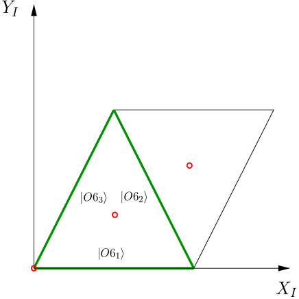
The two different fundamental cycles, around which the branes are wrapping $n_{I}$ and $m_{I}$ times, shall be defined as follows111The difference as compared to the toroidal $\Omega R$-orientifold is an unavoidable consequence of the crystallographic $\mathbb{Z}_{3}$-symmetry.:

(3.5) $$e_{1}^{\bf A}=e_{1}^{\bf B}=R,\quad e_{2}^{\bf A}={R\over 2}+i{\sqrt{3}R\over 2},\quad e_{2}^{\bf B}={R\over 2}+i{R\over 2\sqrt{3}},$$

for each $T^{2}$. The action of $\Omega R$ for both A- and B-torus on the wrapping numbers is given by the map

(3.6) $\displaystyle n_{I}^{\prime}=n_{I}+m_{I}\ ,$
$\displaystyle m_{I}^{\prime}=-m_{I}\ .$

Accordingly, the $\mathbb{Z}_{3}$-action is expressed by the map (differing by $b_{I}=0$ or $b_{I}=1/2$ for the A- and B-torus, respectively)

(3.7) $\displaystyle n_{I}^{\prime}=-\left(1+2b_{I}\right)n_{I}-m_{I}\ ,$
$\displaystyle m_{I}^{\prime}=\left(1+4b_{I}\right)n_{I}+2b_{I}m_{I}\ .$

The six branes contained in the equivalence class $[(n_{I},m_{I})]$ for either A- or B-torus are given by:

(3.8)
$\bigg{(}\begin{array}[]{c}n_{I}\\ m_{I}\end{array}\bigg{)}$ ${\buildrel\mathbb{Z}_{3}\over{\Rightarrow}}$ $\bigg{(}\begin{array}[]{c}-(1+2b_{I})n_{I}-m_{I}\\ (1+4b_{I})n_{I}+2b_{I}m_{I}\end{array}\bigg{)}$ ${\buildrel\mathbb{Z}_{3}\over{\Rightarrow}}$ $\bigg{(}\begin{array}[]{c}2b_{I}n_{I}+m_{I}\\ -(1+4b_{I})n_{I}-(1+2b_{I})m_{I}\end{array}\bigg{)}$
$\ \Omega R\Downarrow$ $\qquad\qquad\ \Omega R\Downarrow$ $\qquad\qquad\ \ \Omega R\Downarrow$
$\bigg{(}\begin{array}[]{c}n_{I}+m_{I}\\ -m_{I}\end{array}\bigg{)}$ ${\buildrel\mathbb{Z}_{3}\over{\Leftarrow}}$ $\bigg{(}\begin{array}[]{c}2b_{I}n_{I}+(2b_{I}-1)m_{I}\\ -(1+4b_{I})n_{I}-2b_{I}m_{I}\end{array}\bigg{)}$ ${\buildrel\mathbb{Z}_{3}\over{\Leftarrow}}$ $\bigg{(}\begin{array}[]{c}-(1+2b_{I})n_{I}-2b_{I}m_{I}\\ (1+4b_{I})n_{I}+(1+2b_{I})m_{I}\end{array}\bigg{)}\ .$


The equivalence class $[(2,1)]$ is shown for for the A-torus as an example in figure 3.2.

Refer to caption
Figure 3.2: The orbit of the exemplary brane $(2,1)$ on the A-torus.

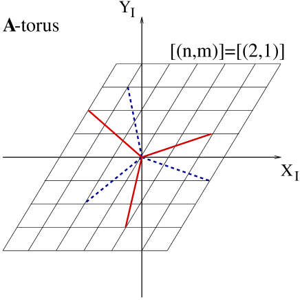
There is a very helpful simplification in the $\mathbb{Z}_{3}$-model, being that only untwisted sector fields couple to the orientifold planes. This is due to the relation

(3.9) $$\Theta\,(\Omega R)=(\Omega R)\,\Theta^{-1},$$

stating the non-commutativity of the two operators $\Omega R$ and $\Theta$ which appear in the trace. Another simple argument is that the orientifold planes are of codimension one on each $T^{2}$ and therefore can avoid a blown-up $\mathbb{P}^{1}$ from an orbifold fixed point. Similarly, the D6-branes can not wrap around the blown-up cycles222Such branes are called fractional branes and will become very important for the $\mathbb{Z}_{4}$-orientifold. and thus they are not charged under the twisted sector RR-fields. As a direct consequence, there will be only untwisted tadpoles in the $\mathbb{Z}_{3}$-orientifold (corresponding to untwisted sectors in the tree channel). Note, that this is a special feature of this model and will not be the case for the $\mathbb{Z}_{4}$-orientifold.

The R-R and NS-NS tadpoles can be calculated following the procedure from the two sections 2.1.5 and 2.1.6 with the alterations that are being described in section 2.2.1.

As the betti number divided by two is equal to one, $\text{b}_{3}/2=1+h_{2,1}=1$, there will be only one R-R and one NS-NS tadpole for the $\mathbb{Z}_{3}$-orientifold.

3.2 R-R tadpole

Klein bottle

Let us start with the Klein-bottle amplitude. The amplitude in the loop channel is given by

(3.10) $$\mathcal{K}^{\text{(NS-NS,$-$)}}=4c\int\limits_{0}^{\infty}\frac{dt}{t^{3}}\text{Tr}_{\text{U+T}}^{\text{(NS-NS,$-$)}}\left(\frac{\Omega R}{2}\ \frac{1+\Theta+\Theta^{2}}{3}\frac{1+(-1)^{F}}{2}\ e^{-2\pi t\mathcal{H}_{\text{closed}}}\right),$$

In the untwisted sector, all insertions $1$, $\Theta$ and $\Theta^{2}$ yield the same contribution, because the lattice Hamiltonian $\mathcal{H}_{\text{lattice}}$ is $\mathbb{Z}_{3}$-invariant. Using $\mathcal{H}_{\text{lattice}}$ (D.14), the untwisted contribution takes the form:

(3.11) $$\mathcal{K}^{\text{(NS-NS,$-$)}}_{\text{U}}=c\int\limits_{0}^{\infty}\frac{dt}{t^{3}}\frac{-\vartheta\bigg{[}{\begin{array}[]{*{20}c}0\\ 1/2\\ \end{array}}\bigg{]}^{4}}{\eta^{12}}\prod_{I=1}^{3}\left[\sum_{r_{I},s_{I}}e^{-\pi t\left(4\frac{{s_{I}}^{2}\alpha^{\prime}}{{R_{I}}^{2}}+\left(3-\frac{16}{3}\,b_{I}\right)\frac{{r_{I}}^{2}{R_{I}}^{2}}{\alpha^{\prime}}\right)}\right],$$

where $b_{I}$ can be again chosen separately for every torus to be 00 or $1/2$. The modular transformation to the tree channel leads to

(3.12) $$\widetilde{\mathcal{K}}^{\text{(R-R,$+$)}}_{\text{U, 1st part}}=-24\sqrt{3}c\int\limits_{0}^{\infty}{dl}\frac{\vartheta\bigg{[}{\begin{array}[]{*{20}c}1/2\\ 0\\ \end{array}}\bigg{]}^{4}}{\eta^{12}}\\ \cdot\left[\prod_{I=1}^{3}\frac{1}{\sqrt{9-16\,b_{I}}}\sum_{r_{I},s_{I}}e^{-4\pi l\left(\frac{{R_{I}}^{2}}{4\alpha^{\prime}}+\frac{3\alpha^{\prime}}{\left(9-16\,b_{I}\right){R_{I}}^{2}}\right)}\right]\ ,$$

where we have to keep in mind that this is just the first part of the untwisted tree channel R-R sector, as the twisted loop channel sectors contribute as well,

(3.13) $$\widetilde{\mathcal{K}}^{\text{(R-R,$+$)}}_{\text{U}}=\widetilde{\mathcal{K}}^{\text{(R-R,$+$)}}_{\text{U, 1st part}}+\widetilde{\mathcal{K}}^{\text{(R-R,$+$)}}_{\text{U, 2nd part}}\ .$$

The contribution of the twisted loop channel sectors transformed to the tree channel is given by

(3.14) $$\widetilde{\mathcal{K}}^{\text{(R-R,$+$)}}_{\text{U, 2nd part}}=-24\sqrt{3}c\int\limits_{0}^{\infty}{dl}\\ \left(\gamma_{1}e^{3\pi i}\,\frac{\vartheta\bigg{[}{\begin{array}[]{*{20}c}1/2\\ 0\\ \end{array}}\bigg{]}\vartheta\bigg{[}{\begin{array}[]{*{20}c}1/2\\ -1/3\\ \end{array}}\bigg{]}\vartheta\bigg{[}{\begin{array}[]{*{20}c}1/2\\ -1/3\\ \end{array}}\bigg{]}\vartheta\bigg{[}{\begin{array}[]{*{20}c}1/2\\ -1/3\\ \end{array}}\bigg{]}}{\eta^{3}\vartheta\bigg{[}{\begin{array}[]{*{20}c}1/2\\ 2/3-1/2\\ \end{array}}\bigg{]}\vartheta\bigg{[}{\begin{array}[]{*{20}c}1/2\\ 2/3-1/2\\ \end{array}}\bigg{]}\vartheta\bigg{[}{\begin{array}[]{*{20}c}1/2\\ 2/3-1/2\\ \end{array}}\bigg{]}}\right.\\ \left.+\gamma_{2}e^{3\pi i}\,\frac{\vartheta\bigg{[}{\begin{array}[]{*{20}c}1/2\\ 0\\ \end{array}}\bigg{]}\vartheta\bigg{[}{\begin{array}[]{*{20}c}1/2\\ 1/3\\ \end{array}}\bigg{]}\vartheta\bigg{[}{\begin{array}[]{*{20}c}1/2\\ 1/3\\ \end{array}}\bigg{]}\vartheta\bigg{[}{\begin{array}[]{*{20}c}1/2\\ 1/3\\ \end{array}}\bigg{]}}{\eta^{3}\vartheta\bigg{[}{\begin{array}[]{*{20}c}1/2\\ 4/3-1/2\\ \end{array}}\bigg{]}\vartheta\bigg{[}{\begin{array}[]{*{20}c}1/2\\ 4/3-1/2\\ \end{array}}\bigg{]}\vartheta\bigg{[}{\begin{array}[]{*{20}c}1/2\\ 4/3-1/2\\ \end{array}}\bigg{]}}\right)\ ,$$

where

(3.15) $$\gamma_{1}=2^{3}\sin(2\pi/3)=3\sqrt{3}\qquad\text{and}\qquad\gamma_{2}=2^{3}\sin(4\pi/3)=-3\sqrt{3}$$

has to be required in order to cancel the bosonic zero modes. The Klein bottle tadpole can be obtained by the zeroth order term in the series expansion of (3.13) using $q=e^{-4\pi l}$:

(3.16) $$T^{\text{R-R}}_{\widetilde{\mathcal{K}}}=-288{\frac{\sqrt{3}c}{\sqrt{9-16\,b_{1}}\sqrt{9-16\,b_{2}}\sqrt{9-16\,b_{3}}}}\ .$$

The normalization of a single orientifold plane (2.31) can be obtained from only $\widetilde{\mathcal{K}}^{\text{(R-R,$+$)}}_{\text{U, 1st part}}$. This term has to be divided by three, as it contains the sum of the three distinct O6-planes. It is given by

(3.17) $$\mathcal{N}_{\text{O6}}=2\,{\frac{\sqrt[4]{3}\sqrt{c}}{\sqrt[4]{9-16\,b_{1}}\sqrt[4]{9-16\,b_{2}}\sqrt[4]{9-16\,b_{3}}}}\ .$$
Cylinder

The cylinder amplitude for a single stack of $N$ $D6$-branes of the equivalence class $[i]$ contains 36 different contributions, six for each open string end which can end on any of the branes within the equivalence class of the model,

(3.18) $$\mathcal{A}=\sum_{j\in[i]}\sum_{k\in[i]}\mathcal{A}_{jk}\ .$$

In order to find the correct normalization factor for a single brane within an equivalence class, we have to calculate the cylinder amplitude only for the sector $\mathcal{A}_{ii}$, where an open string goes from this single brane onto itself. At this time, the brane location should not be specified, so the wrapping numbers $n_{I}$ and $m_{I}$ on each torus are kept arbitrarily and the amplitude of interest for a stack of $N$ branes is given by

(3.19) $$\mathcal{A}_{ii}^{\text{(NS,$-$)}}=c\int\limits_{0}^{\infty}\frac{dt}{t^{3}}\text{Tr}_{\text{D6i-D6i}}^{\text{(NS,$-$)}}\left(\frac{1}{2\cdot 3}\frac{1+(-1)^{F}}{2}e^{-2\pi t\mathcal{H}_{\text{open}}}\right)\ .$$

Using the open string lattice Hamiltonian (D.18), this easily can be calculated to be

(3.20) $$\mathcal{A}_{ii}^{\text{(NS,$-$)}}=\frac{c}{12}N^{2}\int\limits_{0}^{\infty}\frac{dt}{t^{3}}\frac{-\vartheta\bigg{[}{\begin{array}[]{*{20}c}0\\ 1/2\\ \end{array}}\bigg{]}^{4}}{\eta^{12}}\prod_{I=1}^{3}\left[\sum_{r_{I},s_{I}}e^{-\pi t\left(\frac{\frac{2{r_{I}}^{2}}{{R_{I}}^{2}}+\left(\frac{3}{2}-\frac{8}{3}\,b_{I}\right){s_{I}}^{2}{R_{I}}^{2}}{L_{I}^{i}}\right)}\right]\ ,$$

where $L_{I}^{i}$ is the length of the D6-brane on the $I$-th torus

(3.21) $\displaystyle L_{I}^{i}=\sqrt{{n_{I}^{i}}^{2}+n_{I}^{i}\,m_{I}^{i}+\left(1-\frac{4}{3}b_{I}\right){m_{I}^{i}}^{2}}\ .$

Transforming (3.20) into the tree channel R-sector leads to the following normalization of a single brane

(3.22) $$\mathcal{N}_{\text{D6}}=\frac{\sqrt[4]{3}}{2}\,\frac{\,N\sqrt{c}L_{1}^{i}\,L_{2}^{i}\,L_{3}^{i}}{\sqrt[4]{9-16\,b_{1}}\sqrt[4]{9-16\,b_{2}}\sqrt[4]{9-16\,b_{3}}}\ .$$

The sectors of a string between another D-brane of the equivalence class and itself can be obtained by mapping the wrapping numbers $n_{I}$ and $m_{I}$ on every torus according to (3.8), and the result is that all contributions are equal. The cylinder contributions between two D-branes at a non-vanishing do not have to be calculated explicitly in order to determine the tadpole.

Möbius strip

Next, we are going to determine the Möbius strip amplitude in the tree channel. For one stack of branes, the relevant sectors are in between one of the three O6-planes and one of the 6 branes contained within its equivalence class. Due to the $\mathbb{Z}_{3}$-symmetry, it is sufficient to calculate the sector between a certain O6-brane and the sum over the orbit of one arbitrary stack of branes,

(3.23) $$\widetilde{\mathcal{M}}_{[i]}^{\text{(R,$+$)}}=\pm N\int\limits_{0}^{\infty}{dl}\ 2\cdot 2\cdot 3\ \mathcal{N}_{\text{D6}}\ \mathcal{N}_{\text{O6}}\ \\ \cdot\sum_{j\in[i]}\gamma_{j}\ \frac{\vartheta\bigg{[}{\begin{array}[]{*{20}c}1/2\\ 0\\ \end{array}}\bigg{]}\vartheta\bigg{[}{\begin{array}[]{*{20}c}1/2\\ -\kappa_{1}^{j}\\ \end{array}}\bigg{]}\vartheta\bigg{[}{\begin{array}[]{*{20}c}1/2\\ -\kappa_{2}^{j}\\ \end{array}}\bigg{]}\vartheta\bigg{[}{\begin{array}[]{*{20}c}1/2\\ -\kappa_{3}^{j}\\ \end{array}}\bigg{]}}{\vartheta\bigg{[}{\begin{array}[]{*{20}c}1/2\\ 1/2-\kappa_{1}^{j}\\ \end{array}}\bigg{]}\vartheta\bigg{[}{\begin{array}[]{*{20}c}1/2\\ 1/2-\kappa_{2}^{j}\\ \end{array}}\bigg{]}\vartheta\bigg{[}{\begin{array}[]{*{20}c}1/2\\ 1/2-\kappa_{3}^{j}\\ \end{array}}\bigg{]}\eta^{3}}\ .$$

In this amplitude, the one factor of 2 cones from the two spin structures, one factor of 2 from the exchangeability of the bra- and cat-vectors and the factor 3 from the three O6-planes. The contribution of every summand in the sum over the orbit at lowest order is given by

(3.24) $$16\prod_{I=1}^{3}\cos(\pi\kappa_{I}^{j})=16\prod_{I=1}^{3}{\frac{n_{I}^{j}\,n_{I}^{\text{O}}+\left(1-\frac{4}{3}\,b_{I}\right)m_{I}^{j}\,m_{I}^{\text{O}}+\frac{1}{2}\,n_{I}^{j}\,m_{I}^{\text{O}}+\frac{1}{2}\,m_{I}^{j}\,n_{I}^{\text{O}}}{L_{I}^{j}\,L_{I}^{\text{O}}}}\ ,$$

Taking the sum over the orbit in (3.23) and using the property of the perfect square together with (3.16), (3.17) and (3.22), finally leads to the R-R tadpole cancellation equation

(3.25) $$\sum_{a=1}^{k}\,N_{a}\Big{[}{n_{1}^{a}}{n_{2}^{a}}{n_{3}^{a}}\\ +\frac{1}{2}{n_{1}^{a}}{n_{2}^{a}}{m_{3}^{a}}+\frac{1}{2}{n_{1}^{a}}{n_{3}^{a}}{m_{2}^{a}}+\frac{1}{2}{n_{2}^{a}}{n_{3}^{a}}{m_{1}^{a}}-\frac{1}{6}{n_{1}^{a}}{m_{2}^{a}}{m_{3}^{a}}\left(3-6{b_{2}}-6{b_{3}}+8{b_{2}}{b_{3}}\right)\\ -\frac{1}{6}{n_{2}^{a}}{m_{1}^{a}}{m_{3}^{a}}\left(3-6{b_{1}}-6{b_{3}}+8{b_{1}}{b_{3}}\right)-\frac{1}{6}{n_{3}^{a}}{m_{1}^{a}}{m_{2}^{a}}\left(3-6{b_{1}}-6{b_{2}}+8{b_{1}}{b_{2}}\right)\\ -\frac{1}{3}{m_{1}^{a}}{m_{2}^{a}}{m_{3}^{a}}\left(3-3{b_{1}}-3{b_{2}}-3{b_{3}}+2{b_{1}}{b_{3}}+2{b_{1}}{b_{2}}+2{b_{2}}{b_{3}}\right)\Big{]}=2\ .$$

Here, the tadpole cancellation condition already has been generalized for the case of $k$ different stacks, each containing $N_{a}$ branes. For the four tori AAA, AAB, ABB and BBB, this result matches exactly the explicit expressions given in [64]. Later it will turn out to be useful to define the following two quantities for any equivalence class $[(n^{I}_{a},m^{I}_{a})]$ of D6a-branes:

(3.26) $\displaystyle Z_{[a]}={2\over 3}\sum_{({n}_{I}^{b},{m}_{I}^{b})\in[a]}\prod_{I=1}^{3}\left({n}_{I}^{b}+{1\over 2}\,{m}_{I}^{b}\right)\ ,$
$\displaystyle Y_{[a]}=-{1\over 2}\sum_{({n}_{I}^{b},{m}_{I}^{b})\in[a]}(-1)^{M}\,\prod_{I=1}^{3}{m}_{I}^{b}\ ,$

where $M$ is defined to be odd for a mirror brane and otherwise even. The sums are taken over all the individual D6b-branes that are elements of the orbit $[a]$. Then the R-R tadpole equation can be written as

(3.27) $$\sum_{a=1}^{K}N_{a}\,Z_{[a]}=2\ ,$$

because $Z_{[a]}$ is nothing but the expression within the bracket $[\ldots]$ in (3.25). A simple interpretaion for this quantity is the projection of the entire orbit of D6a-branes onto the $X_{I}$ axes, i.e. the sum of their RR charges with respect to the dual D9-brane charge. The RR-charges of all D6-branes have to cancel the RR-charges of the orientifold O6-planes.

Comparing this result with the supersymmetric solutions of [38, 39], an important difference can be seen. Whereas in the supersymmetric case all $Z_{[a]}$ are positive (implying a very small rank of the gauge group), here the $Z_{[a]}$ may also be negative such that gauge groups of a higher rank (as for instance three) might be realized.

3.3 NS-NS tadpole

The NS-NS tadpole can be calculated in a similar manner, if one makes the changes compared to the R-R tadpole that are being described in much detail within section 2.1.6. The result is simply given by

(3.28) $$\langle\phi\rangle_{D}\sim{\partial V\over\partial\phi}$$

with a scalar potential

(3.29) $$V(\phi)=e^{-\phi}\left(\sum_{a}N_{a}\prod_{I=1}^{3}\sum_{j\in[a]}L_{I}^{j}-2\right)\ ,$$

and the length of a certain D6-brane given in (3.21). That there is just one NS-NS tadpole can directly be understood by the fact that all scalars related to the complex structure moduli are projected out under $\mathbb{Z}_{3}$. Consequently, only the dilaton itself can have a disc tadpole. Similar to the toroidal $\Omega R$-orientifold of chapter 2.1.6, whenever the D-branes do not lie on top of the orientifold planes the dilaton tadpole does not vanish. This means that the local cancellation of the R-R charge is in one to one correspondence with supersymmetric vacua and the cancellation of NS-NS tadpoles. The only exception to this rule appears to be a parallel displacement of orientifold planes and D-branes, or in other words a Higgs mechanism breaking $SO(2N_{a})$ to $U(N_{a})$.

3.4 Massless spectrum

The massless spectrum consists of a chiral part, localized at the brane intersections, and a non-chiral part. The chiral spectrum can be determined by methods of topology as described in section 2.3.2. Applying table 2.6 to the $\mathbb{Z}_{3}$-Orientifold leads to the spectrum shown in table 3.1.

Representation Multiplicity
$[{\bf A_{a}}]_{L}$ $Y_{[a]}$
$[{\bf A_{a}+S_{a}}]_{L}$ $Y_{[a]}\left(Z_{[a]}-{1\over 2}\right)$
$[{\bf(\overline{N}_{a},N_{b})}]_{L}$ $Z_{[a]}\,Y_{[b]}-Y_{[a]}\,Z_{[b]}$
$[{\bf(N_{a},N_{b})}]_{L}$ $Z_{[a]}\,Y_{[b]}+Y_{[a]}\,Z_{[b]}$
Table 3.1: The $d=4$ massless chiral spectrum for the $\mathbb{Z}_{3}$-Orientifold.

In addition to these chiral matter fields, the open strings stretching in between the a certain brane $D6_{a}$ and its two $\mathbb{Z}_{3}$ images yield massless fermions in the adjoint representation

(3.30) $$({\rm Adj})_{L}:\quad 3^{n_{\bf B}}\prod_{I=1}^{3}\left(L_{I}^{[a]}\right)^{2}\ ,$$

where $n_{\bf B}$ stands for the number of B-tori in $T^{6}$. This non-chiral sector is ${\cal N}=1$ supersymmetric, as the $\mathbb{Z}_{3}$ rotation on its own preserves supersymmetry. Nevertheless, it will be very important for our phenomenological discussions: for instance, let D6b1 and D6b2 be two different branes in the orbit $[b]$ and D6a another one in the orbit $[a]$. If there is a chiral fermion $\psi_{a,b1}$ in the $(\o{N}_{a},N_{b})$ representation within the D$6_{a}$-D$6_{b1}$ sector and a fermion $\psi_{a,b2}$ in the conjugate $({N}_{a},\o{N}_{b})$ representation within the D$6_{a}$-D$6_{b2}$ sector, then these might pair up to yield a Dirac mass term with a mass of the order of the string scale. The three-point coupling on the disc diagram as shown in figure 3.3 indeed does exist, because in the sector D$6_{b1}$-D$6_{b2}$ there is this massless scalar $H_{b1,b2}$ in the adjoint representation (3.30) of $U(N_{b})$.

Refer to caption
Figure 3.3: The appearance of a dirac mass term in the $\mathbb{Z}_{3}$ orientifold.

If one by hand gives a vacuum expectation value to the $SU(N_{b})$ singlet in the adjoint representation of $U(N_{b})$, then the gauge symmetry is left unbroken the fermions receive a mass. Such a deformation in string theory corresponds to the situation, where two intersecting branes of the orbit $[b]$ are deformed into a single brane wrapping a supersymmetric cycle [110].

3.4.1 Anomaly cancellation

The $SU(N_{a})$ gauge anomalies cancel in the same manner as shown in the general case by the R-R tadpole equation, being described in chapter 2.4.1. For the $U(1)_{a}-g_{\mu\nu}^{2}$, $U(1)_{a}-U(1)_{b}^{2}$ and $U(1)_{a}-SU(N)_{b}^{2}$ anomalies, the Green-Schwarz mechanism has to be employed. Its success in cancelling all these anomalies has been proven generally in chapter 2.4.2. Here, these cancelled $U(1)_{a}-g_{\mu\nu}^{2}$ anomalies are proportional to

(3.31) $$3\,N_{a}\,Y_{[a]}\ ,$$

and the mixed $U(1)_{a}-U(1)_{b}^{2}$ anomalies are given by

(3.32) $$2\,N_{a}\,N_{b}\,Y_{[a]}Z_{[b]}\ .$$

There is only one anomalous $U(1)$,

(3.33) $$F_{\rm mass}=\sum_{a}(N_{a}\,Y_{[a]})\,F_{a}\ ,$$

becoming massive due to the second Chern-Simons coupling in (2.79).

3.4.2 Stability

The complex structure moduli are getting projected out of the scalar potential (3.29), which consequently is flat for the remaining moduli, only the dilaton is not being stabilized, as for the toroidal $\Omega R$-orientifold. Still in higher loop diagrams, we expect that the Kähler moduli to contribute and correct the geometry.

Another stability issue concerns the existence of open string tachyons, which also may spoil stability at the open string loop-level. In general, the bosons of lowest energy in a non-supersymmetric open string sector can have negative mass squared. Here one has to distinguish two different cases. Either the two D-branes in question intersect under a non-trivial angle on all three two-dimensional tori or the D-branes are parallel on at least one of the 2-tori. In the latter case one can get rid of the tachyons at least classically by making the distance between the two D-branes on the $I$-th 2-torus large enough. In the former case, it depends on the three angles, $\varphi_{ab}^{I}$, between the branes D$6_{a}$ and D$6_{b}$ whether there appear tachyons or not.

Defining as usual $\kappa^{ab}_{I}=\varphi_{ab}^{I}/\pi$ and let $P_{ab}$ be the number of $\kappa^{ab}_{I}$ satisfying $\kappa^{ab}_{I}>1/2$, to compute the ground state energy in this twisted open string sector, one has to distinguish the following three cases:

(3.34) $$E^{0}_{ab}=\begin{cases}{1\over 2}\sum_{I}|\kappa^{ab}_{I}|-{\rm max}\left\{|\kappa^{ab}_{I}|\right\}&\text{for}\ P_{ab}=0,1\ ,\vspace{0.3cm}\\ 1+{1\over 2}\left(|\kappa^{ab}_{I}|-|\kappa^{ab}_{J}|-|\kappa^{ab}_{K}|\right)\\ -{\rm max}\left\{|\kappa^{ab}_{I}|,1-|\kappa^{ab}_{J}|,1-|\kappa^{ab}_{K}|\right\}&\text{for}\ P_{ab}=2\ \text{and}\ |\kappa^{ab}_{I}|\leq{1\over 2}\ ,\vspace{0.3cm}\\ 1-{1\over 2}\sum_{I}|\kappa^{ab}_{I}|&\text{for}\ P_{ab}=3\ .\end{cases}$$

In order for a brane model to be free of tachyons, for all open string sectors $E^{0}_{ab}\geq 0$ has to be satisfied. Since in the orbifold model each brane comes with a whole equivalence class of branes, and the angles between two branes do not depend on any moduli, freedom of tachyons is a very strong condition. We will come back to this point in the next section.

3.5 Phenomenological model building

Every potentially interesting model at first has to satisfy the R-R tadpole condition (3.27). Amazingly, even in this fairly constrained orbifold set-up it is not too difficult to get three generation models with $SU(3)\times SU(2)_{L}\times U(1)_{Y}\times U(1)_{B-L}$ or $SU(5)\times U(1)$ gauge groups and standard model matter fields enhanced by a right-handed neutrino. The open string tachyon, being present in many explicit examples, has been suggested to have the interpretation of a Higgs particle, although this seems problematic because this is surely an off-the-mass-shell process and better should be described by open string field theory. In the context of intersecting D-branes, not much is known about these processes.

There are several papers [84, 59, 60] where three generation intersecting brane worlds have been realized on four stacks of D6-branes with gauge group $U(3)\times U(2)\times U(1)\times U(1)$ and chiral matter only in the bifundamental representations of the gauge factors.

This realization is not possible for the $\mathbb{Z}_{3}$ orientifold: requiring that there does not exist any matter in the antisymmetric representation of $U(3)$ forces $Y_{1}=0$. This implies on the other hand using table 3.1 that there are the same number of chiral fermions in the $({\bf 3,2})$ and in the $({\bf\bar{3},2})$ representation of $U(3)\times U(2)$, leading to an even number of left-handed quarks. So we will have to find a different way.

3.5.1 Semi-realistic extended standard model

In order to find a standard-like model, we have to implement two important requirements:

  1. 1.

    The right-handed $(u,c,t)$-quarks have to be in the antisymmetric representation of $U(3)$. For the specific $\mathbb{Z}_{3}$-spectrum, it is similar to the anti-fundamental representation $\bf\bar{3}$.

  2. 2.

    There should not appear any chiral matter in the symmetric representation of $U(3)$ and $U(2)$. This requirement demands $Z_{3}=Z_{2}=1/2$.

From these two conditions, it seems to be possible to approach the standard model with only three initial stacks of D6-branes with gauge group $U(3)\times U(2)\times U(1)$ and the specific choices for the parameters $Y_{a}$ and $Z_{a}$ as given in table 3.2, which indeed fulfills the R-R tadpole cancellation condition.

Initial stack $D6_{a}$ $Y_{a}$ $Z_{a}$
$U(3)$ 3 $\frac{1}{2}$
$U(2)$ 3 $\frac{1}{2}$
$U(1)$ 3 $-\frac{1}{2}$
Table 3.2: The initial stacks for the extended standard model.

The chiral massless 3 generation spectrum can be found in table 3.3.

Matter Representation $SU(3)\times SU(2)\times U(1)^{3}$ $U(1)_{Y}$ $U(1)_{B-L}$
$\left(Q_{L}\right)_{i}$ bifundamental $({\bf 3},{\bf 2})_{(1,1,0)}$ ${1\over 3}$ ${1\over 3}$
$\left(u^{c}_{L}\right)_{i}$ $\bar{A}[U(3)]$ $(\bar{\bf 3},{\bf 1})_{(2,0,0)}$ $-{4\over 3}$ $-{1\over 3}$
$\left(d^{c}_{L}\right)_{i}$ anti-fundamental $(\bar{\bf 3},{\bf 1})_{(-1,0,1)}$ ${2\over 3}$ $-{1\over 3}$
$\left(l_{L}\right)_{i}$ bifundamental $({\bf 1},{\bf 2})_{(0,-1,1)}$ ${-1}$ ${-1}$
$\left(e^{+}_{L}\right)_{i}$ $A[U(2)]$ $({\bf 1},{\bf 1})_{(0,2,0)}$ ${2}$ ${1}$
$\left(\nu^{c}_{L}\right)_{i}$ $\bar{S}[U(1)]$ $({\bf 1},{\bf 1})_{(0,0,-2)}$ ${0}$ ${1}$
Table 3.3: Left-handed fermions of the 3 stack Standard-like model.

The non-chiral spectrum will not be treated in this section, as it is assumed that the non-chiral fermions have paired up and have decoupled. By the Green-Schwarz mechanism, the expected anomalous U(1) is given by

(3.35) $$U(1)_{\rm mass}=3\,U(1)_{1}+2\,U(1)_{2}+U(1)_{3}\ ,$$

and between the anomaly-free ones, one can choose the specific linear combination

(3.36) $\displaystyle U(1)_{Y}$ $\displaystyle=-{2\over 3}\,U(1)_{1}+U(1)_{2},$
$\displaystyle U(1)_{B-L}$ $\displaystyle=-{1\over 6}\left(U(1)_{1}-3\,U(1)_{2}+3\,U(1)_{3}\right)\ .$

to be also anomaly-free, which coincidentally are the hypercharge and another extended $B-L$ symmetry. The $B-L$ decouples, but still survives as a global symmetry. The possible Yukawa couplings by this fact are more constrained than in the standard model.

Since the one-loop consistency of the string model requires the formal cancellation of the $U(2)$ and $U(1)$ (non-abelian) gauge anomalies, the possible models are fairly constrained and require the introduction of right-handed neutrinos, being a strong prediction of these type of models. Because the lepton number is not a global symmetry of the model, there exists the possibility to obtain Majorana mass terms and invoke the see-saw mechanism for the neutrino mass hierarchy.

Of course, so far, we have not given any concrete realization of these models in terms of their winding numbers $n_{I}$ and $m_{I}$. In order to do so, a computer program has been set up, searching for winding numbers in between -10 and 10 that realize the given $Y_{a}$ and $Z_{a}$. The tachyon conditions, being described in chapter 3.4.2, have been checked for every model, and it has turned out that one could find 36 solutions for every single one of the 3 stacks, independently of the choice of torus. Another rather mysterious observation could be made: for all models all winding numbers just range in between -3 and 3, and only for the BBB torus from $-5$ and $5$. The actual number of inequivalent string models with the above mentioned standard-like model features then is $4\cdot 36^{3}$.

Gauge breaking

The discussed version of the standard model extended by a gauged $B-L$ symmetry together with right-handed neutrinos requires a two step gauge symmetry breaking in order to serve as a realistic model, see for instance [111]. In order to avoid conflicts with various experimental facts, one has to require a hierarchy of Higgs vacuum expectation values.

First of all, the $U(1)_{B-L}$ has to be broken at a scale at least $\sim 10^{4-6}$ above the electroweak scale. This requires a Higgs field charged under this group but a singlet otherwise. This could be met by a tachyon from a sector of strings stretching between two branes in the orbit that supports the $U(1)_{3}$. We will embark this strategy in the following section, although it has to be said that this process should better be described by string field theory, as it is an off-shell process and the endpoint of this tachyon condensation process so far cannot be determined on general grounds.

Secondly, the familiar electroweak symmetry breaking which needs a bifundamental Higgs doublet has to find an explanation within the discussed model.

Tachyons

It has to be distinguished between tachyons in different sectors of our model: when the two branes are in different equivalence classes $[a]$ and $[b]$, the tachyonic Higgs field is in the bifundamental representation of the $U(N_{a})\times U(N_{b})$ gauge group and the condensation resembles the Higgs mechanism of electroweak symmetry breaking. On the contrary, when the two branes are elements of the same orbit $[a]$, the Higgs field will be in the antisymmetric, symmetric or adjoint representation of the $U(N_{a})$ and thus affect only this factor.

A study among all the $4\cdot 36^{3}$ models looking for a suitable tachyon spectrum has been performed. In any sector of open strings stretching between two D6-branes $a$ and $b$ the lightest physical state has a mass given by (3.34). By expressing the angle variables in terms of winding numbers, a computer program has been set up to search for models with a Higgs scalar in the $({\bf 2,1})$ and/or another one in the ‘symmetric’ representation of $U(1)_{B-L}$. All other open string sectors need to be free of tachyons. The results of this search are listed in table 3.4.

Model $U(3)$ $[U(3),U(2)]$ $[U(3),U(1)]$ $U(2)$ $[U(2),U(1)]$ $U(1)$ $\#$
AAA $\times$ $\times$ $\times$ $\times$ $-$ $-$ 384
AAA $\times$ $\times$ $\times$ $\times$ $\times$ $-$ 384
AAA $\times$ $\times$ $\times$ $\times$ $\times$ $\times$ 0
AAB $\times$ $\times$ $\times$ $\times$ $-$ $-$ 16320
AAB $\times$ $\times$ $\times$ $\times$ $\times$ $-$ 10944
AAB $\times$ $\times$ $\times$ $\times$ $\times$ $\times$ 10944
ABB $\times$ $\times$ $\times$ $\times$ $-$ $-$ 17472
ABB $\times$ $\times$ $\times$ $\times$ $\times$ $-$ 9024
ABB $\times$ $\times$ $\times$ $\times$ $\times$ $\times$ 9024
BBB $\times$ $\times$ $\times$ $\times$ $-$ $-$ 768
BBB $\times$ $\times$ $\times$ $\times$ $\times$ $-$ 768
BBB $\times$ $\times$ $\times$ $\times$ $\times$ $\times$ 384
Table 3.4: Freedom from tachyons for all sectors between either branes of the same or different equivalence classes and the number $\#$ of complying models. $\times$ denotes freedom from tachyons in the specific sector, $-$ means that the tachyon condition is unchecked.

Some important observations can be made from this table:

  1. 1.

    For the AAA and the BBB type tori one can get D6-brane configurations that display only tachyons charged under $U(1)_{B-L}$, but none of these models does have a suitable tachyon in the $({\bf 2,1})$. Vice versa, the AAB and ABB models do have Higgs fields in the $({\bf 2,1})$ but no singlets charged under $U(1)_{B-L}$.

  2. 2.

    For all tori except the ${\bf AAA}$ type, one can even set up D6-brane configurations without tachyons at all.

  3. 3.

    There are several hundred models having either a tachyon in $({\bf 2,1})$ or a tachyon in the ‘symmetric’ representation of $U(1)_{B-L}$. On the other hand, none of the models contains both tachyons, what seems to be discouraging at first sight. Regarding the necessity to have a hierarchy of a high scale breaking of $U(1)_{B-L}$ and a low scale electroweak Higgs mechanism, we are forced to choose a model with a singlet tachyon condensing at the string scale but without any Higgs field in the $({\bf 2,1})$. This favors an alternative mechanism for electroweak symmetry breaking. An explicit realization is for example given by

    (3.37) $\displaystyle[(n_{1}^{I},m_{1}^{I})]$ $\displaystyle=[(-3,2),(0,1),(0,-1)],$
    $\displaystyle[(n_{2}^{I},m_{2}^{I})]$ $\displaystyle=[(-3,2),(0,1),(0,-1)],$
    $\displaystyle[(n_{3}^{I},m_{3}^{I})]$ $\displaystyle=[(-3,2),(1,-1),(-1,0)].$

    This model has precisely 3 Higgs singlets

    (3.38) $$h_{i}:\qquad({\bf 1,1})_{(0,0,-2)}\ ,$$

    carrying only $B-L$ charge but no hypercharge. They are former ‘superpartners’ of the right-handed neutrinos.

  4. 4.

    Another astonishing result turns out while examining the possible solutions to the tadpole equations: those models displaying the Higgs singlet charged under $U(1)_{B-L}$ and no tachyons otherwise, result from a model with a gauge group $SU(5)\times U(1)$, deformed by giving a vacuum expectation value to a scalar in the adjoint of $SU(5)$. Geometrically, this is evident in the fact that the stacks of branes that support the $SU(3)$ and $SU(2)_{L}$ are always parallel, thus their displacement is a marginal deformation at tree level. Of course, we have to expect that quantum corrections will generate a potential for the respective adjoint scalar.

Yukawa couplings

There is one important deviation of the discussed model from the standard model: due to the additional global symmetries, an appropriate Yukawa coupling giving a mass to the $(u,c,t)$-quarks is absent. This can be seen from the quantum numbers of the Higgs field $\tilde{H}$. It can be determined regarding the relevant Yukawa coupling

(3.39) $$\tilde{H}\,\bar{Q}_{L}\,u_{R}\ .$$

Gauge invariance forces $\tilde{H}$ to have the quantum numbers

(3.40) $$\tilde{H}:\qquad({\bf 1,2})_{(3,1,0)}\ .$$

Unfortunately, no microscopic open string state can transform in the singlet representation of $U(3)$ and at the same time have a $U(1)$ charge $q=3$. On the other hand, the relevant Yukawa coupling for the $(d,s,b)$ quarks and the leptons is given by

(3.41) $$H\,\bar{Q}_{L}\,d_{R},\qquad H\,\bar{l}_{L}\,e_{R},\qquad H^{*}\,\bar{l}_{L}\,\nu_{R},$$

leading to the quantum numbers $({\bf 1,2})_{(0,1,1)}$ for the Higgs fields $H$. This is not in contradiction to the open string origin of the model.

From this observation, one has to draw the conclusion that in open string models where the $(u,c,t)$-quarks arise from open strings in the antisymmetric representation of $U(3)$, the usual Higgs mechanism does not apply. The only solution to this problem appears to be replacing the fundamental Higgs scalar by an alternative composite operator, possessing the quantum numbers stated in (3.40).

In order to end this section, the generation of neutrino masses shall be discussed. A scalar $h$ in the ‘symmetric’ representation of the $U(1)_{3}$ can break the $U(1)_{B-L}$ symmetry via the Higgs mechanism. This does not directly lead to a Yukawa coupling of Majorana type for the right moving neutrinos. However, the dimension five coupling

(3.42) $${1\over M_{s}}\,\left(h^{*}\right)^{2}\,\left(\bar{\nu}^{c}\right)_{L}\,\nu_{R}$$

is invariant under all global symmetries and leads to a Majorana mass for the right moving neutrinos. Together with the predicted composite Higgs mechanism for the standard Higgs field this might allow the realization of the see-saw mechanism in order to generate small neutrino masses.

Weinberg angle

The $U(N_{a})$ gauge couplings can be obtained by simple dimensional reduction. This leads to

(3.43) $${4\pi^{2}\over g_{a}^{2}}={M_{s}\over g_{s}}\prod_{I=1}^{3}L_{a}^{I}\ ,$$

where $g_{s}$ is the string coupling. The gauge coupling for the hypercharge

(3.44) $$Q_{Y}=\sum_{a}c_{a}\,Q_{a}$$

generally is given by

(3.45) $${1\over g_{Y}^{2}}=\sum_{a}{1\over 4}{c_{a}\over g_{a}^{2}}\ ,$$

if the the normalization tr$(Q_{a}^{2})=1/2$ is used for the abelian subgroups $U(1)_{a}\subset U(N_{a})$. For our specific model, this yields a Weinberg angle

(3.46) $$\sin^{2}\vartheta_{W}={3\over 6+2{g_{2}\over g_{1}}}\ ,$$

where the hypercharge in terms of the correctly normalized $U(1)$s, denoted by a tilde, is given by

(3.47) $$Q_{Y}=-{2\over 3}U(1)_{1}+U(1)_{2}=-{2\over 3}\sqrt{6}\,\widetilde{U(1)}_{1}+2\,\widetilde{U(1)}_{2}\ .$$

Since in all interesting cases the $U(3)$ branes have the same internal volumes like the $U(2)$ branes, (3.46) reduces to the prediction $\sin^{2}\vartheta_{W}=3/8$, which is precisely the $SU(5)$ GUT result. This indeed gives a strong prediction for any $\mathbb{Z}_{3}$ orbifold model, different as compared to the examples on toroidal orbifolds [60], where the complex structure moduli also play an important role.

Proton decay

One of the most important obstacles any phenomenological standard-like model has to overcome is a possible proton decay. Indeed, in the discussed model only the combination $B-L$ appears as a symmetry, so that there are potential problems with the stability of the proton. Following [102], as long as the quark fields appear in bifundamental representations of the stringy gauge group, the proton is stable because effective couplings with three quarks are forbidden. This argument does not apply in the present case.

Refer to caption
Figure 3.4: Generation of a dimension six coupling.

In figure 3.4, it is shown that a disc diagram can generate a dimension six coupling

(3.48) $${\cal L}\sim{1\over M_{s}^{2}}\left(\bar{u}^{c}_{L}\,u_{L}\right)\,\left(\bar{e}^{+}_{L}\,d_{L}\right),$$

preserving $B-L$ but violating baryon and lepton numbers separately. The numbers at the boundary indicate the D6a-brane to which the boundary of the disc is attached.

The conclusion which can be drawn from this observation is that as long as the large extra dimension scenario is assumed yielding a string scale $M_{s}\ll 10^{16}$GeV, there is a serious problem with proton decay. This result certainly advocates a string scale at the GUT scale opposite to one at the TeV scale.

3.5.2 Flipped $SU(5)\times U(1)$ GUT model

This section gives a reinterpretation of the extended standard-like model of the last section as a GUT scenario. Similar models can be found in [112]. The unified model in our case can be obtained from the standard-like model by moving the two stacks for the $U(2)$ and $U(3)$ sector on top of each other, or in other words, by giving a vanishing VEV to the adjoint Higgs 24.

In this realization, the common GUT gauge group $SU(5)$ is extended by a single gauged $U(1)$ symmetry. On two stacks of branes with $N_{5}=5$ and $N_{1}=1$ the model is realized by picking again

(3.49) $$(Y_{5},Z_{5})=\left(3,{1\over 2}\right),\qquad(Y_{1},Z_{1})=\left(3,-{1\over 2}\right).$$

The task of expressing these effective winding numbers in terms of $[(n_{a}^{I},m_{a}^{I})]$ quantum numbers is identical to that for the previously discussed extended standard model. The number of solutions is again 36 for each stack, yielding a total set of $4\cdot 36^{2}$ inequivalent models. The chiral fermion spectrum is given in table 3.5.

Number $SU(5)\times U(1)^{2}$ $U(1)_{\text{free}}$
$3$ $(\bar{\bf 5},{\bf 1})_{(-1,1)}$ $-{6\over 5}$
$3$ $({\bf 10},{\bf 1})_{(2,0)}$ ${2\over 5}$
$3$ $({\bf 1},{\bf 1})_{(0,-2)}$ ${-2}$
Table 3.5: Left-handed fermions of the flipped $SU(5)\times U(1)$ model.

The Green-Schwarz mechanism yields an anomalous $U(1)$ which is given by

(3.50) $$U(1)_{\text{mass}}=5\,U(1)_{5}+U(1)_{1}\ ,$$

in accordance with (3.33), and the anomaly-free one is

(3.51) $$U(1)_{\text{free}}={1\over 5}\,U(1)_{5}-U(1)_{1}\ ,$$

This is the desired field content of a grand unified standard model with additional right-handed neutrinos. Consequently, the model fits into $SO(10)$ representations. The usual minimal Higgs sector consists of the adjoint 24 to break $SU(5)$ to $SU(3)\times SU(2)_{L}\times U(1)_{Y}$ and a $({\bf 5,1})$ which produces the electroweak breaking. In addition we now also need to have a singlet to break the extra $U(1)_{\rm free}$ gauge factor. The adjoint scalar is present as being a part of the vectormultiplet of the formerly ${\cal N}=4$ supersymmetric sector of strings starting and ending on identical branes within the stack $[5]$. Turning on a VEV in the supersymmetric theory means moving on the Coulomb branch of the moduli space, which geometrically translates into separating the five $D6_{5}$-branes into parallel stacks of two and three branes. The form of the potential generated for this modulus after supersymmetry breaking is not known, and the existence of a negative mass term, being required for the spontaneous condensation, remains speculative.

After having identified the $SU(5)$ GUT as a standard model where two stacks of branes are pushed upon each other, it can be referred to the former analysis of the scalar spectrum for the other two needed Higgs fields. The results of the search for Higgs singlets and bifundamentals done for the $SU(3)\times SU(2)_{L}\times U(1)_{Y}\times U(1)_{B-L}$ model within the previous chapter apply without modification, as the two stacks for $SU(3)\times SU(2)_{L}$ are parallel in all cases. In [113] it was realized that the discussed model actually is a flipped $SU(5)$ model.

Similarly to the standard-like model, here the $U(1)_{\text{mass}}$ does not allow Yukawa couplings of the type ${\bf 10\cdot 10\cdot 5}$. Again the standard mass generation mechanism does not work. Gauge symmetry breaking and mass generation have to be achieved proposing a composite Higgs fields with the right quantum numbers.

Chapter 4 The MSSM on the $\mathbb{Z}_{4}$-orientifold

In this chapter, we will concentrate on the construction of supersymmetric orientifold models. In recent times, it often has been stressed (see for instance [114]) that a concrete realization of a model from string theory, having exactly the matter content of the MSSM without any additional exotic matter and at the same time $\mathcal{N}$=1 supersymmetry, still is missing. On the other hand, such a model might be much more predictive than just effective supergravity. Therefore, maybe it could already be tested within the next generation of particle accelerators, or concretely, the LHC.

The $\mathbb{Z}_{4}$-orbifold, containing also fractional D-branes, is particularly useful for this purpose. In the end, a 3-generation Pati-Salam model will be discussed in detail. It is shown that it can be broken down to a MSSM-like model, involving several brane recombination mechanisms.

4.1 The $\mathbb{Z}_{4}$-orbifold

The following model will be discussed in this chapter:

(4.1) $${{\text{Type\ IIA}}\ {\text{on}}\ T^{6}\over\{\mathbb{Z}_{4}+\Omega R\mathbb{Z}_{4}\}}.$$

The left-right symmetric $\mathbb{Z}_{4}$ orbifold shall act as

(4.2) $\displaystyle\Theta_{1}:\qquad Z_{1}\to e^{\pi i/2}\,Z_{1}$
$\displaystyle\Theta_{2}:\qquad Z_{2}\to e^{\pi i/2}\,Z_{2}$
$\displaystyle\Theta_{3}:\qquad Z_{3}\to e^{-\pi i}\,Z_{3}$

on the three complex coordinates, assuming again a factorization of the 6-torus by $T^{6}=T^{2}\times T^{2}\times T^{2}$. Indeed, (4.2) corresponds to one case given in the cyclic orbifold classification in table 2.4, so this action in the closed string sector preserves $\mathcal{N}$=2 supersymmetry in four dimensions without and $\mathcal{N}$=1 together with the orientifold projection $\Omega R$. Consequently, the orbifold can be seen as a singular limit of a Calabi-Yau threefold.

An important observation from (4.2) is that the orbifold action on the first two tori is a $\mathbb{Z}_{4}$- rotation, whereas that on the last torus is a $\mathbb{Z}_{2}$-rotation. As a direct consequence, the first two tori have to be rectangular and therefore, the complex structure on these tori is fixed to $U_{2}=1$.

There are again two inequivalent choices for the each 2-torus, in the T-dual picture corresponding to a vanishing or non-vanishing constant NS-NS 2-form flux. Again, they shall be called A- and B-torus. In the preceding chapters, the orientifold projection always has been chosen for both tori in such a way that it was reflecting along the X-axis and besides, the B-torus was tilted. Instead, one can choose the B-torus to be rectangular, but at the same time take a different choice for the anti-holomorphic involution $R$:

(4.3) $\displaystyle{\bf A}:\ Z_{i}{\buildrel R\over{\longrightarrow}}\overline{Z}_{i}$
$\displaystyle{\bf B}:\ Z_{i}{\buildrel R\over{\longrightarrow}}e^{\frac{\pi i}{2}}\overline{Z}_{i}\ .$

For reasons of simplicity, we will choose this convention on the first two tori and on the third torus the usual one (meaning a tilted B-torus). This choice is shown together with the $\Omega R$ fixed point sets in figure 4.1.

Refer to caption
Figure 4.1: The anti-holomorphic involutions and conventions on the three 2-tori for the $\mathbb{Z}_{4}$ orientifold.

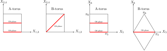
As a consequence, the complex structure on the 3rd torus is given by $U=iU_{2}$ for the A-torus with $U_{2}$ unconstrained and by $U=1/2+iU_{2}$ for the B-torus.

By combining all possible choices of complex conjugations, one obtains eight possible orientifold models. However, taking into account that the orientifold model on the $\mathbb{Z}_{4}$ orbifold does not only contain the orientifold planes related to $\Omega R$ but likewise the orientifold planes related to $\Omega R\Theta$, $\Omega R\Theta^{2}$ and $\Omega R\Theta^{3}$, only the four models AAA, ABA, AAB and ABB are different.

The hodge numbers of this threefold are given by $h_{2,1}=7$ and $h_{1,1}=31$, where the number $h_{2,1}=7$ corresponds to the number of complex structure and $h_{1,1}=31$ to the number of Kähler deformations. These moduli are coming from the following sectors:

  • untwisted sector: As two complex structures are fixed, another unconstrained one from the third torus remains in the untwisted sector. Furthermore, there are 5 Kähler moduli in this sector, where in each case two are coming from the first and second trorus, one from the last.

  • $\Theta$ and $\Theta^{3}$ twisted sectors: These two sectors together give rise to 16 Kähler moduli, because they do contain 16 $\mathbb{Z}_{4}$-fixed points.

  • $\Theta^{2}$ twisted sector: In this sector, there are 16 $\mathbb{Z}_{2}$-fixed points from which 4 are also $\mathbb{Z}_{4}$-fixed points. Just the $\mathbb{Z}_{4}$-fixed points give rise to one Kähler modulus each. The remaining twelve $\mathbb{Z}_{2}$-fixed points are organized in pairs under the $\mathbb{Z}_{4}$ action and so give rise to 6 complex structure and 6 Kähler moduli.

The $\mathbb{Z}_{2}$-twisted sector contributes $h^{tw}_{2,1}=6$ elements to the number of complex structure deformations and therefore contains twisted 3-cycles, which is the important new feature of this $\mathbb{Z}_{4}$ orbifold compared to the $\mathbb{Z}_{3}$ of the preceding chapter.

4.2 An integral basis for $H_{3}(M,\mathbb{Z})$

It would be very tedious to determine the tadpoles and the massless chiral spectrum of this model by a pure CFT calculation, as in the present case twisted sector tadpoles contribute as well. So we will take a different route and use the description in terms of homology that has been introduced in the two chapters 2.1.5 and 2.3.2. The R-R tadpole reads in terms of homology

(4.4) $$\sum_{a}N_{a}\,(\pi_{a}+\pi^{\prime}_{a})-4\,\pi_{O6}=0.$$

As a first step, we have to determine the independent 3-cycles on the $\mathbb{Z}_{4}$ orbifold space. The third betti number is given by $b_{3}=2+2h_{21}=16$, so one expects to get precisely this number of independent 3-cycles, if one does not consider the $\Omega R$ projection at this point.

The first set of these cycles can be obtained easily, as it descends from the ambient toroidal space $T^{6}$. The two fundamental cycles on the torus $T^{2}_{I}$ ($I=1,2,3$) shall be denoted as $\pi_{2I-1}$ and $\pi_{2I}$. Then the toroidal 3-cycles can be defined by

(4.5) $$\pi_{ijk}\equiv\pi_{i}\otimes\pi_{j}\otimes\pi_{k}\ .$$

If we take the orbits under the $\mathbb{Z}_{4}$ action, we can immediately deduce four $\mathbb{Z}_{4}$-invariant 3-cycles,

(4.6) $\displaystyle\rho_{1}$ $\displaystyle\equiv 2(\pi_{135}-\pi_{245}),\qquad\bar{\rho}_{1}\equiv 2(\pi_{136}-\pi_{246}),$
$\displaystyle\rho_{2}$ $\displaystyle\equiv 2(\pi_{145}+\pi_{235}),\qquad\bar{\rho}_{2}\equiv 2(\pi_{146}+\pi_{236})\ .$

The factor of two comes from the fact that $1$ and $\Theta^{2}$ as well as $\Theta$ and $\Theta^{3}$ act equivalently on the toroidal cycles. The intersection matrix on the orbifold space for these 3-cycles can be obtained from equation (2.71). It is given by

(4.7) $$I_{\rho}=\bigoplus_{i=1}^{2}\left(\begin{matrix}0&-2\\ 2&0\\ \end{matrix}\right)\ .$$

We are still missing twelve 3-cycles, these do arise in the $\mathbb{Z}_{2}$ twisted sector of the orbifold. Since $\Theta^{2}$ acts non-trivially only onto the first two 2-tori, the sixteen $\mathbb{Z}_{2}$-fixed points do appear in the $\mathbb{Z}_{2}$ twisted sector on these tori, this is shown in figure 4.2.
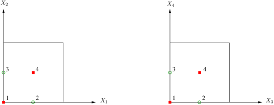
Refer to caption
Figure 4.2: The $\mathbb{Z}_{4}$ orbifold fixed points on the first two $T^{2}$.

The boxes in the figure indicate the $\mathbb{Z}_{2}$-fixed points which are also fixed under the $\mathbb{Z}_{4}$ symmetry, the circles indicate the ones that are just fixed under the $\mathbb{Z}_{2}$ and get exchanged under the $\mathbb{Z}_{4}$ action.

After blowing up the orbifold singularities, each of these fixed points gives rise to an exceptional 2-cycle $e_{ij}$ with the topology of $S^{2}$. These exceptional 2-cycles can be combined with the two fundamental 1-cycles on the third torus (indicated by $\pi_{5}$ and $\pi_{6}$ in figure 4.1) to form what might be called exceptional 3-cycles with the topology of $S^{2}\times S^{1}$. But the $\mathbb{Z}_{4}$ action leaves only four fixed points invariant and arranges the remaining twelve in six pairs. Since it acts by a reflection on the third torus, its action on the exceptional cycles $e_{ij}\otimes\pi_{5,6}$ is given by

(4.8) $$\Theta\left(e_{ij}\otimes\pi_{5,6}\right)=-e_{\theta(i)\theta(j)}\otimes\pi_{5,6}\ ,$$

where

(4.9) $$\theta(1)=1,\quad\theta(2)=3,\quad\theta(3)=2,\quad\theta(4)=4\ .$$

The $\mathbb{Z}_{4}$-invariant fixed points drop out because of the minus sign in (4.8) and exactly twelve 3-cycles remain, being

(4.10) $\displaystyle\varepsilon_{1}$ $\displaystyle\equiv(e_{12}-e_{13})\otimes\pi_{5}\ ,\qquad\bar{\varepsilon}_{1}\equiv(e_{12}-e_{13})\otimes\pi_{6}\ ,$
$\displaystyle\varepsilon_{2}$ $\displaystyle\equiv(e_{42}-e_{43})\otimes\pi_{5}\ ,\qquad\bar{\varepsilon}_{2}\equiv(e_{42}-e_{43})\otimes\pi_{6}\ ,$
$\displaystyle\varepsilon_{3}$ $\displaystyle\equiv(e_{21}-e_{31})\otimes\pi_{5}\ ,\qquad\bar{\varepsilon}_{3}\equiv(e_{21}-e_{31})\otimes\pi_{6}\ ,$
$\displaystyle\varepsilon_{4}$ $\displaystyle\equiv(e_{24}-e_{34})\otimes\pi_{5}\ ,\qquad\bar{\varepsilon}_{4}\equiv(e_{24}-e_{34})\otimes\pi_{6}\ ,$
$\displaystyle\varepsilon_{5}$ $\displaystyle\equiv(e_{22}-e_{33})\otimes\pi_{5}\ ,\qquad\bar{\varepsilon}_{5}\equiv(e_{22}-e_{33})\otimes\pi_{6}\ ,$
$\displaystyle\varepsilon_{6}$ $\displaystyle\equiv(e_{23}-e_{32})\otimes\pi_{5}\ ,\qquad\bar{\varepsilon}_{6}\equiv(e_{23}-e_{32})\otimes\pi_{6}\ .$

Using (2.71), the resulting intersection matrix for the exceptional cycles takes the simple form

(4.11) $$I_{\varepsilon}=\bigoplus_{i=1}^{6}\left(\begin{matrix}0&-2\\ 2&0\\ \end{matrix}\right)\ .$$

These cycles do not form an integral basis of the free module, although being part of the homology group $H_{3}(M,\mathbb{Z})$. The reason is that their intersection matrix is not unimodular.

On the other hand, it is possible to obtain an integral basis: Concerning the physical interpretation, what we are missing are the so-called fractional D-branes that first have been described in [115, 116]. Regarding our model, these are D-branes which only wrap one-half times around any toroidal cycle $\rho_{1}$, $\bar{\rho}_{1}$, $\rho_{2}$ or $\bar{\rho}_{2}$ and at the same time wrap around some of the exceptional cycles in the blown-up manifold. In the orbifold limit they are stuck at the fixed points and at least two such branes have to combine to form a normal D-brane that can move into the bulk.

At this point, we have to clarify which combinations of toroidal and exceptional cycles are possible for a fractional D-brane. This can be figured out as follows: if a D-brane wraps around a toroidal cycle, it passes through one or two of the $\mathbb{Z}_{2}$-fixed points. It seems reasonable that only these fixed points are able to contribute to the fractional brane. For instance, if a brane wraps the toroidal cycle $1/2\,\rho_{1}$, then only the exceptional cycles $\epsilon_{1}$, $\epsilon_{3}$ or $\epsilon_{5}$ should be allowed. The total homological cycle then could be for instance

(4.12) $$\pi_{a}={1\over 2}\rho_{1}+{1\over 2}(\varepsilon_{1}+\varepsilon_{3}+\varepsilon_{5})\ .$$

From these simple considerations, we cannot fix the relative signs of the different terms in (4.12). An interpretation for these signs is given by the correspondence to Wilson lines along an internal direction of the D-brane, which we are free to turn on. Indeed, this construction is completely analogous to the construction of boundary states for fractional D-branes carrying also a charge under some $\mathbb{Z}_{2}$ twisted sector states [73, 117, 118, 119].

Therefore, only unbarred respectively barred cycles can be combined into fractional cycles, as they wrap the same fundamental 1-cycle on the third 2-torus. Then the only non-vanishing intersection numbers are in between barred and unbarred cycles.

Any unbarred fractional D-brane can be expanded as

(4.13) $$\pi_{a}=v_{a,1}\rho_{1}+v_{a,2}\rho_{2}+\sum_{i=1}^{6}v_{a,i+2}\,\varepsilon_{i}\ ,$$

where the coefficients $v_{a,i}$ are half-integer valued. We can associate to it a barred brane by simply exchanging the two fundamental cycles on the third 2-torus

(4.14) $$\bar{\pi}_{a}=v_{a,1}\bar{\rho}_{1}+v_{a,2}\bar{\rho}_{2}+\sum_{i=1}^{6}v_{a,i+2}\,\bar{\varepsilon}_{i}\ ,$$

having the same coefficients $v_{a,i+8}=v_{a,i}$ for $i\in\{1,\ldots,8\}$.

Now, all linear combinations with an intersection number $\pi\circ\bar{\pi}=-2$ can be constructed if we respect the rules given above. This provides a basis for the homology lattice. The cycles respecting $\pi\circ\bar{\pi}=-2$ can be divided into three sets:

  1. 1.

    $\{(v_{1},v_{2};v_{3},v_{4};v_{5},v_{6};v_{7},v_{8})\\ \text{with}\ v_{1}+v_{2}=\pm\frac{1}{2},\,v_{3}+v_{4}=\pm\frac{1}{2},\,v_{5}+v_{6}=\pm\frac{1}{2},\,v_{7}+v_{8}=\pm\frac{1}{2},\\ \text{and}\ v_{1}+v_{3}+v_{5}+v_{7}=0\ {\rm mod}\ 1\}$

    These combinations correspond to flat branes being parallel to the fundamental cycles which intersect through certain fixed points. They define $8\cdot 16=128$ different fractional 3-cycles.

  2. 2.

    $\{(v_{1},v_{2};v_{3},v_{4};0,0;0,0),\,(v_{1},v_{2};0,0;v_{5},v_{6};0,0),\,(v_{1},v_{2};0,0;0,0;v_{7},v_{8}),\\ (0,0;v_{3},v_{4};v_{5},v_{6};0,0),\,(0,0;v_{3},v_{4};0,0;v_{7},v_{8}),\,(0,0;0,0;v_{5},v_{6};v_{7},v_{8})\\ \text{with}\ v_{i}={\pm 1/2}\}$

    The first three types of elements of this set stretch along one of the toroidal fundamental cycles on one 2-torus and diagonally on the other one. The remaining three types arise from integer linear combinations of the cycles introduced so far. In total this yields $6\cdot 16=96$ different 3-cycles.

  3. 3.

    $\{(v_{1},v_{2};v_{3},v_{4};v_{5},v_{6};v_{7},v_{8})\ \text{with exactly one}\ v_{i}=\pm 1\ \text{and the rest zero}\}$

    Only the vectors with $v_{1}=\pm 1$ or $v_{2}=\pm 1$ can be derived from untwisted branes. They are purely untwisted. The purely twisted ones again arise from linear combinations. This third set contains $2\cdot 8=16$ 3-cycles.

Adding up all possibilities, there are 240 distinct 3-cycles obeying $\pi\circ\bar{\pi}=-2$. Intriguingly, this just corresponds to the number of roots of the $E_{8}$ Lie algebra. Therefore, with the help of a computer program, it is possible to search for a basis among these 240 cycles such that the intersection matrix takes the following form

(4.15) $$I=\left(\begin{matrix}0&C_{E_{8}}\\ -C_{E_{8}}&0\\ \end{matrix}\right)\ ,$$

where $C_{E_{8}}$ denotes the Cartan matrix of $E_{8}$ which is given by

(4.16) $$C_{E_{8}}=\left[\begin{matrix}-2&1&0&0&0&0&0&0\\ 1&-2&1&0&0&0&0&0\\ 0&1&-2&1&0&0&0&0\\ 0&0&1&-2&1&0&0&0\\ 0&0&0&1&-2&1&0&1\\ 0&0&0&0&1&-2&1&0\\ 0&0&0&0&0&1&-2&0\\ 0&0&0&0&1&0&0&-2\\ \end{matrix}\right]\ .$$

A typical solution that has been found is given by

$\displaystyle\vec{v}_{1}$ $\displaystyle={1\over 2}(-1,\phantom{-}0,-1,\phantom{-}0,-1,\phantom{-}0,-1,\phantom{-}0)$
$\displaystyle\vec{v}_{2}$ $\displaystyle={1\over 2}(\phantom{-}1,\phantom{-}0,\phantom{-}1,\phantom{-}0,\phantom{-}1,\phantom{-}0,-1,\phantom{-}0)$
$\displaystyle\vec{v}_{3}$ $\displaystyle={1\over 2}(\phantom{-}1,\phantom{-}0,-1,\phantom{-}0,-1,\phantom{-}0,\phantom{-}1,\phantom{-}0)$
(4.17) $\displaystyle\vec{v}_{4}$ $\displaystyle={1\over 2}(-1,\phantom{-}0,\phantom{-}1,\phantom{-}0,\phantom{-}0,\phantom{-}1,\phantom{-}0,\phantom{-}1)$
$\displaystyle\vec{v}_{5}$ $\displaystyle={1\over 2}(\phantom{-}0,\phantom{-}1,-1,\phantom{-}0,\phantom{-}1,\phantom{-}0,\phantom{-}0,-1)$
$\displaystyle\vec{v}_{6}$ $\displaystyle={1\over 2}(\phantom{-}0,-1,\phantom{-}1,\phantom{-}0,-1,\phantom{-}0,\phantom{-}0,-1)$
$\displaystyle\vec{v}_{7}$ $\displaystyle={1\over 2}(\phantom{-}0,\phantom{-}1,\phantom{-}0,\phantom{-}1,\phantom{-}0,-1,\phantom{-}0,\phantom{-}1)$
$\displaystyle\vec{v}_{8}$ $\displaystyle={1\over 2}(\phantom{-}0,-1,\phantom{-}0,-1,\phantom{-}0,-1,\phantom{-}0,\phantom{-}1).$

Since the Cartan matrix is unimodular, we indeed have constructed by (4.2) an integral basis for the homology lattice $H_{3}(M,\mathbb{Z})$.

In the following, it nevertheless turns out to be more convenient to work with the non-integral orbifold basis which also allows for half-integer coefficients. But one has to be careful in doing so: not all such cycles are part of $H_{3}(M,\mathbb{Z})$, one has to ensure for every apparent fractional 3-cycle that it is indeed part of the unimodular lattice $H_{3}(M,\mathbb{Z})$. This can be achieved by checking if it can be expressed as an integer linear combination of the basis (4.2).

4.3 The $\mathbb{Z}_{4}$-orientifold

In the last section, we have determined an integer basis for the 3-cycles in the $\mathbb{Z}_{4}$ orbifold on the $T^{6}$, but have not treated the orientifold projection $\Omega R$ so far. A first step in doing so is to find the homological 3-cycles which the O6-planes are wrapping, or in other words, determine the fixed point sets of the four relevant orientifold projections $\Omega R$, $\Omega R\Theta$, $\Omega R\Theta^{2}$ and $\Omega R\Theta^{3}$. Here, the exemplary case of the ABB-model will be discussed in detail, as it will be particularly useful for model building. The results for the other cases are listed in the table E.1 of appendix E.1.

4.3.1 The O6-planes for the ABB-orientifold

The fixed points sets can be expressed in terms of the toroidal 3-cycles, as shown in table 4.1.

Projection Fixed point set
$\Omega R$ $2\,\pi_{135}+2\,\pi_{145}$
$\Omega R\Theta$ $2\,\pi_{145}+2\,\pi_{245}-4\,\pi_{146}-4\,\pi_{246}$
$\Omega R\Theta^{2}$ $2\,\pi_{235}-2\,\pi_{245}$
$\Omega R\Theta^{3}$ $-2\,\pi_{135}+2\,\pi_{235}+4\,\pi_{136}-4\,\pi_{236}$
Table 4.1: The O6-planes for the ABB-torus.

By adding up all contributions, one obtains

(4.18) $\displaystyle\pi_{O6}$ $\displaystyle=4\,\pi_{145}+4\,\pi_{235}+4\,\pi_{136}-4\,\pi_{246}-4\,\pi_{146}-4\,\pi_{236}$
$\displaystyle=2\,\rho_{2}+2\,\bar{\rho}_{1}-2\,\bar{\rho}_{2}\ .$

Strikingly, the total O-plane can be expressed in terms of bulk cycles only. This reflects the fact that in the conformal field theory the orientifold planes carry only charge under untwisted R-R fields, as mentioned in chapter 2.2 already.

Next, we are trying to determine the action of $\Omega R$ on the homological cycles. In terms of the orbifold basis, this is just given by

(4.19) $\displaystyle\rho_{1}\to\rho_{2},$ $\displaystyle\bar{\rho}_{1}\to\rho_{2}-\bar{\rho}_{2},$
$\displaystyle\rho_{2}\to\rho_{1},$ $\displaystyle\bar{\rho}_{2}\to\rho_{1}-\bar{\rho}_{1}.$

for the toroidal cycles and by

$\displaystyle\varepsilon_{1}\to-\varepsilon_{1},$ $\displaystyle\bar{\varepsilon}_{1}\to-\varepsilon_{1}+\bar{\varepsilon}_{1},$
$\displaystyle\varepsilon_{2}\to-\varepsilon_{2},$ $\displaystyle\bar{\varepsilon}_{2}\to-\varepsilon_{2}+\bar{\varepsilon}_{2},$
(4.20) $\displaystyle\varepsilon_{3}\to\varepsilon_{3},\phantom{-}$ $\displaystyle\bar{\varepsilon}_{3}\to\varepsilon_{3}-\bar{\varepsilon}_{3},$
$\displaystyle\varepsilon_{4}\to\varepsilon_{4},\phantom{-}$ $\displaystyle\bar{\varepsilon}_{4}\to\varepsilon_{4}-\bar{\varepsilon}_{4},$
$\displaystyle\varepsilon_{5}\to\varepsilon_{6},\phantom{-}$ $\displaystyle\bar{\varepsilon}_{5}\to\varepsilon_{6}-\bar{\varepsilon}_{6},$
$\displaystyle\varepsilon_{6}\to\varepsilon_{5},\phantom{-}$ $\displaystyle\bar{\varepsilon}_{6}\to\varepsilon_{5}-\bar{\varepsilon}_{5}.$

for the exceptional cycles.

4.3.2 Supersymmetric cycles

In this chapter, we are interested in supersymmetric models. Therefore, we do not only need to have control over the topological data of the D6-branes, but also over the nature of the special Lagrangian cycles.

The metric at the orbifold point is flat up to some isolated orbifold singularities. Therefore, flat D6-branes in a given homology class are definitely special Lagrangian. At this time, we restrict the D6-branes to be flat and factorizable in the sense that they can be described by the usual six wrapping numbers along the fundamental toroidal cycles, $n_{I}$ and $m_{I}$ with $I=1,2,3$, which have to be relatively coprime on every 2-torus. Given such a bulk brane, one can easily compute the homology class that it wraps in the orbifold basis

(4.21) $\displaystyle\pi^{\text{bulk}}_{a}=$ $\displaystyle\left[(n_{1}^{a}\,n_{2}^{a}-m_{1}^{a}\,m_{2}^{a})n_{3}^{a}\right]\,\rho_{1}+\left[(n_{1}^{a}\,m_{2}^{a}+m_{1}^{a}\,n_{2}^{a})n_{3}^{a}\right]\,\rho_{2}$
$\displaystyle+$ $\displaystyle\left[(n_{1}^{a}\,n_{2}^{a}-m_{1}^{a}\,m_{2}^{a})m_{3}^{a}\right]\,\bar{\rho}_{1}+\left[(n_{1}^{a}\,m_{2}^{a}+m_{1}^{a}\,n_{2}^{a})m_{3}^{a}\right]\,\bar{\rho}_{2}\ .$

The supersymmetry that the orientifold plane preserves is preserved by a specific D-brane as well if it fulfills the angle criterion: the angles on all tori have to add up to the total angle that the O-plane spans on the three 2-tori. This concretely reads for the ABB-orientifold

(4.22) $$\varphi_{1}^{a}+\varphi_{2}^{a}+\varphi_{3}^{a}={\pi\over 4}\ {\rm mod}\ 2\pi\ ,$$

and the three angles are given by

(4.23) $$\tan\varphi_{1}^{a}={m_{1}^{a}\over n_{1}^{a}}\ ,\qquad\tan\varphi_{2}^{a}={m_{2}^{a}\over n_{2}^{a}}\ ,\qquad\tan\varphi_{3}^{a}={U_{2}\,m_{3}^{a}\over n_{3}^{a}+{1\over 2}m_{3}^{a}}\ ,$$

where we have to keep in mind that only the complex structures on the first two 2-tori are fixed. It is possible to reformulate the criterion (4.22) in terms of wrapping numbers, if one simply takes the tangent on both sides of the equation. But we have to be careful in doing so, as this only yields a necessary condition: the tangent has a periodicity ${\rm mod}\ \pi$. Solving for $U_{2}$ leads to

(4.24) $$U_{2}={\left(n_{3}^{a}+{1\over 2}m_{3}^{a}\right)\over m_{3}^{a}}{\left(n_{1}^{a}\,n_{2}^{a}-m_{1}^{a}\,m_{2}^{a}-n_{1}^{a}\,m_{2}^{a}-m_{1}^{a}\,n_{2}^{a}\right)\over\left(n_{1}^{a}\,n_{2}^{a}-m_{1}^{a}\,m_{2}^{a}+n_{1}^{a}\,m_{2}^{a}+m_{1}^{a}\,n_{2}^{a}\right)}\ .$$

We can interpret this equation in such a way that already one supersymmetric stack of D-brane fixes the complex structure on the third torus. The introduction of additional D6-branes gives rise to non-trivial conditions on the wrapping numbers of these D-branes. For the other three orientifold models, these supersymmetry conditions are listed in appendix E.2.

Later we want to construct a supersymmetric model containing also fractional branes in order to enlarge the model building possibilities. The explicit expression in terms of wrapping numbers takes the following form

(4.25) $$\pi_{a}^{\text{frac}}={1\over 2}\pi_{a}^{\text{bulk}}+{n_{3}^{a}\over 2}\left[\sum_{j=1}^{6}w_{a,j}\varepsilon_{j}\right]+{m_{3}^{a}\over 2}\left[\sum_{j=1}^{6}w_{a,j}\bar{\varepsilon}_{j}\right]\qquad\text{with}\ w_{a,j}\in\{-1,0,1\}\ .$$

In terms of the formerly introduced coefficients $v_{a,j}$, this reads

(4.26) $$v_{a,j}={n_{3}^{a}\over 2}\,w_{a,j},\qquad\quad v_{a,j+8}={m_{3}^{a}\over 2}\,w_{a,j}\qquad\quad\text{for}\ j\in\{1,\ldots,8\}\ .$$

In 4.25 we have taken into account that all the $\mathbb{Z}_{2}$-fixed points are located on the first two 2-tori: on the third torus fractional D-branes do have winding numbers along the two fundamental 1-cycles. Moreover, the coefficients of $\varepsilon_{j}$ and $\bar{\varepsilon}_{j}$ in (4.25) must be equal, because they only differ by the cycle on the third torus.

Using the same determination principles for the normalization factors as for the toroidal $\Omega R$- and $\mathbb{Z}_{3}$ orientifolds111These are determined by the Cardy condition, stating that the result for the annulus partition function must coincide for the loop and the tree channel computation., these fractional D6-branes correspond to the following boundary states in the conformal field theory of the $T^{6}/\mathbb{Z}_{4}$ orbifold model

(4.27) $$|D^{f};(n_{I},m_{I}),\alpha_{ij}\rangle={1\over 2\sqrt{2}}\sqrt{n_{3}^{2}+n_{3}m_{3}+{\textstyle{m_{3}^{2}\over 2}}}\\ \cdot\left[\bigg{(}\frac{1}{2}\prod_{j=1}^{2}\sqrt{n_{j}^{2}+m_{j}^{2}}\bigg{)}\bigg{(}\bigl{|}D;(n_{I},m_{I})\bigr{\rangle}_{U}+\bigl{|}D;\Theta(n_{I},m_{I})\bigr{\rangle}_{U}\bigg{)}\right.\\ \left.+\bigg{(}\sum_{i,j=1}^{4}\alpha_{ij}\bigl{|}D;(n_{I},m_{I}),e_{ij}\bigr{\rangle}_{T}+\sum_{i,j=1}^{4}\alpha_{ij}\bigl{|}D;\Theta(n_{I},m_{I}),\Theta(e_{ij})\bigr{\rangle}_{T}\bigg{)}\right]\ .$$

In this boundary state, there are contributions from both the untwisted and the $\mathbb{Z}_{2}$-twisted sector and we have taken the orbit under the $\mathbb{Z}_{4}$ action, being for the winding numbers

(4.28) $\displaystyle\Theta\,n_{1,2}=-m_{1,2}\ ,$ $\displaystyle\Theta\,m_{1,2}=n_{1,2}\ ,$
$\displaystyle\Theta\,n_{3}=-n_{3}\ ,$ $\displaystyle\Theta\,m_{3}=-m_{3}\ .$

implying that $\Theta^{2}$ acts like the identity on the boundary states. This explains why only two and not four untwisted boundary states do appear in (4.27). In the sum over the $\mathbb{Z}_{2}$-fixed points, for each D6-brane precisely four coefficients take values $\alpha_{ij}=\pm 1$ and the remaining ones are vanishing, as these coefficients are directly related to the $w_{i}$ appearing in the description of the corresponding fractional 3-cycles. It has been mentioned already that changing the signs of an exceptional cycle does correspond to turning on a discrete $\mathbb{Z}_{2}$ Wilson line along one internal direction of the brane [119]. The action of $\Theta$ on the twisted sector ground states $e_{ij}$ has been given in (4.8). Furthermore, the elementary boundary states $|D;(n_{I},m_{I})\rangle_{U}$ are the usual ones for a flat $D6$-brane with wrapping numbers $(n_{I},m_{I})$ on a 6-torus factorizing in three 2-tori. They are given in appendix E.3.

$n_{1}$ odd, $m_{1}$ odd $n_{1}$ odd, $m_{1}$ even $n_{1}$ even, $m_{1}$ odd
$n_{2}$ odd $\varepsilon_{3}$, $\varepsilon_{4}$ $\varepsilon_{3}$, $\varepsilon_{4}$
$m_{2}$ odd $\varepsilon_{5}$, $\varepsilon_{6}$ $\varepsilon_{5}$, $\varepsilon_{6}$
$n_{2}$ odd $\varepsilon_{1}$, $\varepsilon_{2}$ $\varepsilon_{1}$, $\varepsilon_{3}$, $\varepsilon_{5}$ $\varepsilon_{1}$, $\varepsilon_{3}$, $\varepsilon_{6}$
$m_{2}$ even $\varepsilon_{5}$, $\varepsilon_{6}$ $\varepsilon_{1}$, $\varepsilon_{4}$, $\varepsilon_{6}$ $\varepsilon_{1}$, $\varepsilon_{4}$, $\varepsilon_{5}$
$\varepsilon_{2}$, $\varepsilon_{3}$, $\varepsilon_{6}$ $\varepsilon_{2}$, $\varepsilon_{3}$, $\varepsilon_{5}$
$\varepsilon_{2}$, $\varepsilon_{4}$, $\varepsilon_{5}$ $\varepsilon_{2}$, $\varepsilon_{4}$, $\varepsilon_{6}$
$n_{2}$ even $\varepsilon_{1}$, $\varepsilon_{2}$ $\varepsilon_{1}$, $\varepsilon_{3}$, $\varepsilon_{6}$ $\varepsilon_{1}$, $\varepsilon_{3}$, $\varepsilon_{5}$
$m_{2}$ odd $\varepsilon_{5}$, $\varepsilon_{6}$ $\varepsilon_{1}$, $\varepsilon_{4}$, $\varepsilon_{5}$ $\varepsilon_{1}$, $\varepsilon_{4}$, $\varepsilon_{6}$
$\varepsilon_{2}$, $\varepsilon_{3}$, $\varepsilon_{5}$ $\varepsilon_{2}$, $\varepsilon_{3}$, $\varepsilon_{6}$
$\varepsilon_{2}$, $\varepsilon_{4}$, $\varepsilon_{6}$ $\varepsilon_{2}$, $\varepsilon_{4}$, $\varepsilon_{5}$
Table 4.2: The allowed exceptional cycles for fractional branes on the torus.

At this point, we want to implement the constraint that only those fractional cycles are able to contribute to the fractional brane (4.25) where the bulk brane is passing through. This can be easily implemented by hand, the result is given in table 4.2. At first glance, there seems to be a mismatch between the number of parameters describing a 3-cycle and the corresponding boundary state: there are three non-vanishing parameters $w_{i}$ but four $\alpha_{ij}$ for every D-brane. But this is misleading, as a flat fractional brane and its $\mathbb{Z}_{4}$-image always intersect in precisely one $\mathbb{Z}_{4}$-fixed point times a circle on the third 2-torus. This twisted sector effectively drops out of the boundary state, because $\Theta$ acts on this fixed point with a minus sign.

This is not merely a coincidence but has a far-reaching physical interpretation: between a brane and its $\Theta$ mirror, there generally lives a hypermultiplet $\Phi_{\text{adj}}$ in the adjoint representation, see equation (3.30). But this sector is non-chiral in four dimensions and $\mathcal{N}$=2 supersymmetric, such that there exists a flat direction in the D-term potential. This implies that the two branes recombine into a single one which no longer passes through the $\mathbb{Z}_{4}$-fixed point, an illustration of this process is given in figure 4.3.

Refer to caption
Figure 4.3: The recombination process of two $\mathbb{Z}_{4}$ mirror branes into a sigle non-flat D-brane.

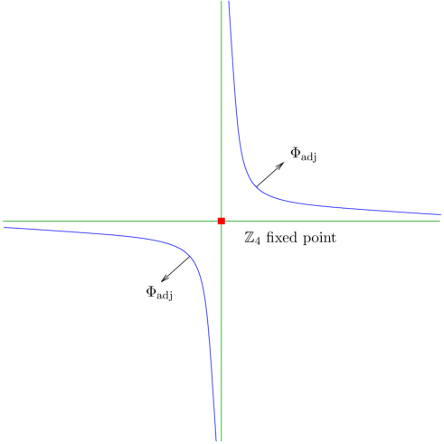
A non-trivial test for these considerations is given by the check if a fractional brane (4.25), transformed to the $E_{8}$-basis, yields integer coefficients. To see this, we write the $8\times 8$ matrix (4.16) and a second identical copy as the two diagonal blocks of a $16\times 16$ matrix, and then act with the inverse of the transposed matrix onto a general vector (4.25). Then we have to investigate the different cases according to table 4.2 separately. For instance for the case $n_{1}$ odd, $n_{2}$ odd, $m_{1}$ even, $m_{2}$ odd and fractional cycles $\varepsilon_{3}$, $\varepsilon_{4}$ with signs $w_{3}$, $w_{4}$ respectively, we substitute $m_{1}=2k_{1}$ and obtain the following vector in the $E_{8}$-basis:

(4.29) $$\bigg{[}\Big{(}{1\over 2}(n_{1}m_{2}-w_{3})+k_{1}n_{2}\Big{)}n_{3},\ \Big{(}{1\over 2}(n_{1}n_{2}-w_{3})-k_{1}m_{2}+n_{1}m_{2}+2k_{1}n_{2}\Big{)}n_{3},\ ...\bigg{]}.$$

Already for the first two components we can see what generally happens for all cases and all components: since $n_{1}$, $n_{2}$, $m_{2}$ and $w_{3}$ are non-vanishing and because products of odd numbers are odd as well, just sums and differences of two odd numbers occur. These are always even or zero and therefore can be divided by two and still lead to integer coefficients. This ends our considerations about supersymmetric fractional D6-branes, and we are ready to search for phenomenologically interesting supersymmetric models.

4.4 Phenomenological model building

In this section, we are interested in supersymmetric extensions of the standard model. The most obvious attempt in model building would be to directly search for a supersymmetric model that has the stacks and intersection numbers as given in chapter 3.5 or [60, 100]. This in general could be achieved for any one of the four models AAA, ABA, AAB and ABB and for a fixed complex structure on the third torus $U_{2}$. The choice of complex structure then by (4.24) restricts the choice for supersymmetric branes. At least fixing $U_{2}$ to a specific value is a legitimate action, because the scalar potential (2.57) for this modulus is vanishing. It corresponds to a stable minimum as we will see from the NS-NS tadpole condition.

In order to do so, a computer program has been set up to search for such a model with wrapping numbers up to ten. This model was required to satisfy both the R-R tadpole equation (4.4) and the supersymmetry condition (4.24) for a flexible number of stacks. Unfortunately, a model with the correct intersection numbers in all sectors in this way could not be found, although its existence cannot be excluded on general grounds. For this reason, in the following we will concentrate on a three generation Pati-Salam model. This can even be broken down by certain mechanisms to a supersymmetric standard-like model. In more detail, this process involves two important steps of first breaking a 7 stack Pati-Salam model down to a 3 stack model using a certain complex structure deformation and then breaking this further down to the supersymmetric standard-like model. This second breaking can be achieved in two different ways, either by an adjoint or by a bifundamental Pati-Salam breaking, both possibilities will be discussed.

Non-supersymmetric Pati-Salam models are discussed in [120, 121]. Another supersymmetric four generation Pati-Salam model has been constructed in [48], but due to its minor phenomenological relevance, it will not be treated in this work.

4.4.1 Seven stack Pati-Salam model

For the ${\bf ABB}$ model with a complex structure of the third torus fixed to be $U_{2}=1/2$, the only mutual intersection numbers that have been found by the computer program are $(\pi_{a}\circ\pi_{b},\pi^{\prime}_{a}\circ\pi_{b})=(0,0),(\pm 1,0),(0,\pm 1)$. This still allows for a construction of a four generation supersymmetric Pati-Salam model with initial gauge groups $U(4)\times U(2)^{3}\times U(2)^{3}$. One typical example is realized by the wrapping number as shown in table 4.3.

Stack $(n_{I},m_{I})$ Homology cycle
U(4) $(1,0;1,0;0,1)$ $\pi_{1}={1\over 2}\left(\bar{\rho}_{1}-\bar{\varepsilon}_{1}-\bar{\varepsilon}_{3}-\bar{\varepsilon}_{5}\right)$
$\pi^{\prime}_{1}={1\over 2}\left(\rho_{2}-\bar{\rho}_{2}+\varepsilon_{1}-\varepsilon_{3}-\varepsilon_{6}-\bar{\varepsilon}_{1}+\bar{\varepsilon}_{3}+\bar{\varepsilon}_{6}\right)$
U(2) $(1,0;1,0;0,1)$ $\pi_{2}={1\over 2}\left(\bar{\rho}_{1}-\bar{\varepsilon}_{1}+\bar{\varepsilon}_{3}+\bar{\varepsilon}_{5}\right)$
$\pi^{\prime}_{2}={1\over 2}\left(\rho_{2}-\bar{\rho}_{2}+\varepsilon_{1}+\varepsilon_{3}+\varepsilon_{6}-\bar{\varepsilon}_{1}-\bar{\varepsilon}_{3}-\bar{\varepsilon}_{6}\right)$
U(2) $(1,0;1,0;0,1)$ $\pi_{3}={1\over 2}\left(\bar{\rho}_{1}-\bar{\varepsilon}_{2}+\bar{\varepsilon}_{3}+\bar{\varepsilon}_{6}\right)$
$\pi^{\prime}_{3}={1\over 2}\left(\rho_{2}-\bar{\rho}_{2}+\varepsilon_{2}+\varepsilon_{3}+\varepsilon_{5}-\bar{\varepsilon}_{2}-\bar{\varepsilon}_{3}-\bar{\varepsilon}_{5}\right)$
U(2) $(1,0;1,0;0,1)$ $\pi_{4}={1\over 2}\left(\bar{\rho}_{1}+\bar{\varepsilon}_{2}+\bar{\varepsilon}_{3}+\bar{\varepsilon}_{6}\right)$
$\pi^{\prime}_{4}={1\over 2}\left(\rho_{2}-\bar{\rho}_{2}-\varepsilon_{2}+\varepsilon_{3}+\varepsilon_{5}+\bar{\varepsilon}_{2}-\bar{\varepsilon}_{3}-\bar{\varepsilon}_{5}\right)$
U(2) $(1,0;1,0;0,1)$ $\pi_{5}={1\over 2}\left(\bar{\rho}_{1}+\bar{\varepsilon}_{1}-\bar{\varepsilon}_{3}+\bar{\varepsilon}_{5}\right)$
$\pi^{\prime}_{5}={1\over 2}\left(\rho_{2}-\bar{\rho}_{2}-\varepsilon_{1}-\varepsilon_{3}+\varepsilon_{6}+\bar{\varepsilon}_{1}+\bar{\varepsilon}_{3}-\bar{\varepsilon}_{6}\right)$
U(2) $(1,0;1,0;0,1)$ $\pi_{6}={1\over 2}\left(\bar{\rho}_{1}+\bar{\varepsilon}_{1}+\bar{\varepsilon}_{4}-\bar{\varepsilon}_{6}\right)$
$\pi^{\prime}_{6}={1\over 2}\left(\rho_{2}-\bar{\rho}_{2}-\varepsilon_{1}+\varepsilon_{4}-\varepsilon_{5}+\bar{\varepsilon}_{1}-\bar{\varepsilon}_{3}+\bar{\varepsilon}_{5}\right)$
U(2) $(1,0;1,0;0,1)$ $\pi_{7}={1\over 2}\left(\bar{\rho}_{1}+\bar{\varepsilon}_{1}-\bar{\varepsilon}_{4}-\bar{\varepsilon}_{6}\right)$
$\pi^{\prime}_{7}={1\over 2}\left(\rho_{2}-\bar{\rho}_{2}-\varepsilon_{1}-\varepsilon_{4}-\varepsilon_{5}+\bar{\varepsilon}_{1}+\bar{\varepsilon}_{3}+\bar{\varepsilon}_{5}\right)$
Table 4.3: The wrapping numbers and homology cycles of the D6-branes in the 7 stack Pati-Salam-model.

The next step is to determine the scalar potential for the modulus $U_{2}$. This cannot be obtained from topological considerations, only from the NS-NS tadpole calculation. For the specific $\mathbb{Z}_{4}$-model in table 4.3, we get a contribution from the O6-plane tension which is given by

(4.30) $${V}_{O6}=-T_{6}\,e^{-\phi_{4}}16\sqrt{2}\left({1\over\sqrt{U_{2}}}+2\sqrt{U_{2}}\right)\ ,$$

and a contribution from the seven stacks of D6-branes:

(4.31) $\displaystyle{V}_{1}$ $\displaystyle=T_{6}\,e^{-\phi_{4}}16\sqrt{{1\over 4\,U_{2}}+U_{2}}\ ,$
$\displaystyle{V}_{2,\ldots,7}$ $\displaystyle=T_{6}\,e^{-\phi_{4}}8\sqrt{{1\over 4\,U_{2}}+U_{2}}\ .$

The sum over all terms,

(4.32) $${V}_{\text{scalar}}={V}_{O6}+\sum_{i=1}^{7}{V}_{i}\ ,$$

is plotted in figure 4.4.

Refer to caption
Figure 4.4: The total scalar potential for $U_{2}$ in the discussed model of table 4.3.

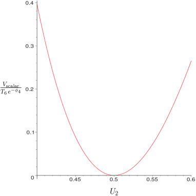
It can be seen in this plot that the scalar potential indeed has a minimum at the value $U_{2}=1/2$. This can be understood as a consistency check for our procedure: supersymmetry really fixes the complex structure on the third torus. This freezing of moduli for supersymmetric backgrounds is very similar to what happens for instance in compactifications with non-vanishing R-R fluxes [122, 123, 124].

Next, we have to determine the massless open string spectrum of the model. In terms of ${\cal N}=2$ supermultiplets, the model contains vector multiplets in the gauge group $U(4)\times U(2)^{3}\times U(2)^{3}$. Beside this, there are two hypermultiplets in the adjoint representation of each unitary gauge factor. The complex scalar in the vector multiplet corresponds to the unconstrained position of each stack of D6-branes on the third 2-torus.

The chiral spectrum can be determined using table 2.6, where the mutual intersection numbers of the cycles (4.3) have to be computed. The result is listed in table 4.4, and one can see that the non-abelian anomalies cancel for this spectrum (including formally also the $U(2)$ anomalies). Neither there are symmetric nor antisymmetric representations, and the bifundamental representations of the type ${\bf(\overline{N}_{a},N_{b})}$ also do not give any net contributions as the corresponding intersection numbers $\pi_{a}\circ\pi_{b}$ vanish.

Field Number $U(4)\times U(2)^{3}\times U(2)^{3}$
$\Phi_{1^{\prime}2}$ 1 $(4;2,1,1;1,1,1)$
$\Phi_{1^{\prime}3}$ 1 $(4;1,{2},1;1,1,1)$
$\Phi_{1^{\prime}4}$ 1 $(4;1,1,{2};1,1,1)$
$\Phi_{1^{\prime}5}$ 1 $(\bar{4};1,1,1;\bar{2},1,1)$
$\Phi_{1^{\prime}6}$ 1 $(\bar{4};1,1,1;1,\bar{2},1)$
$\Phi_{1^{\prime}7}$ 1 $(\bar{4};1,1,1;1,1,\bar{2})$
$\Phi_{2^{\prime}3}$ 1 $(1;\bar{2},\bar{2},1;1,1,1)$
$\Phi_{2^{\prime}4}$ 1 $(1;\bar{2},1,\bar{2};1,1,1)$
$\Phi_{3^{\prime}4}$ 1 $(1;1,\bar{2},\bar{2};1,1,1)$
$\Phi_{5^{\prime}6}$ 1 $(1;1,1,1;2,{2},1)$
$\Phi_{5^{\prime}7}$ 1 $(1;1,1,1;2,1,{2})$
$\Phi_{6^{\prime}7}$ 1 $(1;1,1,1;1,{2},{2})$
Table 4.4: Chiral spectrum of the 7 stack Pati-Salam-model.

This model of course at first glance is a one generation model, but a three generation model can be obtained if the two triplets $U(2)^{3}$ are broken down to their diagonal subgroups. Potential gauge symmetry breaking candidates in this way are the chiral fields $\{\Phi_{2^{\prime}3},\Phi_{2^{\prime}4},\Phi_{3^{\prime}4}\}$ and $\{\Phi_{5^{\prime}6},\Phi_{5^{\prime}7},\Phi_{6^{\prime}7}\}$ from table 4.4. However, one has to remember that these are chiral ${\cal N}=1$ supermultiplets living on the intersection of two D-branes in every case. In order to see which gauge breaking mechanisms are possible, it is necessary to determine the non-chiral spectrum. As explained in chapter 2.3.3, this spectrum cannot be calculated by homology, only by the conformal field theory calculation. This is unproblematic, as we just have to calculate the overlap of two boundary states of the type (4.27) and then transform the result to the loop channel to get the cylinder amplitude (3.18), where we can read off the massless states immediately. This also provides a check for the chiral spectrum.

The non-chiral spectrum first for one stack of $U(2)$ branes contains the usual hypermultiplet $\Phi_{\text{adj}}=(\phi_{adj},\tilde{\phi}_{adj})$ in the adjoint representation of $U(2)$, being localized at the intersection between a brane an its $\Theta$ image (see figure 4.3). Additionally, there are two chiral multiplets $\Psi_{A}$ and $\Psi_{\bar{A}}$, in the ${\bf A}$ respectively ${\bf\bar{A}}$ representation arising from the sector between a brane and its $\Omega R$-mirror. These two fields, carrying the conjugate representations of the gauge group, cannot be seen from the topological intersection number which actually vanishes, $\pi_{i}\circ\pi^{\prime}_{i}=0$. The quiver diagram for these three types of fields is given in figure 4.5.

Refer to caption
Figure 4.5: Adjoint higgsing for the 7 stack Pati-Salam model.

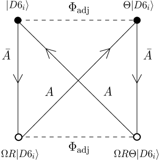
Every closed polygon that is contained in the diagram corresponds to a possible term in the superpotential, that is then made up of the product of the associated fields. In the present case, the following two terms can appear

(4.33) $$W=\phi_{\text{adj}}\Psi_{A}\Psi_{\bar{A}}+\tilde{\phi}_{\text{adj}}\Psi_{A}\Psi_{\bar{A}}\ ,$$

which will generate a mass for the anti-symmetric fields when the adjoint multiplet gets a VEV. But as discussed in chapter 4.3.2, after giving a VEV to the adjoint field, the brane recombines with its $\Theta$ mirror and consequently, this recombined brane does not pass any longer through the fixed point. So the only remaining fields are given by the bifundamentals which are listed in table 4.5.

Field Number $U(4)\times U(2)^{3}\times U(2)^{3}$
$H_{12}$ 1 $(4;\bar{2},1,1;1,1,1)+c.c.$
$H_{13}$ 1 $(4;1,\bar{2},1;1,1,1)+c.c.$
$H_{14}$ 1 $(4;1,1,\bar{2};1,1,1)+c.c.$
$H_{15}$ 1 $(\bar{4};1,1,1;{2},1,1)+c.c.$
$H_{16}$ 1 $(\bar{4};1,1,1;1,{2},1)+c.c.$
$H_{17}$ 1 $(\bar{4};1,1,1;1,1,{2})+c.c.$
$H_{25}$ 1 $(1;{2},1,1;\bar{2},1,1)+c.c.$
$H_{26}$ 1 $(1;{2},1,1;1,\bar{2},1)+c.c.$
$H_{27}$ 1 $(1;{2},1,1;1,1,\bar{2})+c.c.$
$H_{35}$ 1 $(1;1,{2},1;\bar{2},1,1)+c.c.$
$H_{36}$ 1 $(1;1,{2},1;1,\bar{2},1)+c.c.$
$H_{37}$ 1 $(1;1,{2},1;1,1,\bar{2})+c.c.$
$H_{45}$ 1 $(1;1,1,{2};\bar{2},1,1)+c.c.$
$H_{46}$ 1 $(1;1,1,{2};1,\bar{2},1)+c.c.$
$H_{47}$ 1 $(1;1,1,{2};1,1,\bar{2})+c.c.$
Table 4.5: Non-chiral spectrum of the 7 stack Pati-Salam-model.

4.4.2 Three stack Pati-Salam model

It is obvious from table 4.5 that although there are bifundamentals which generally could break down the gauge groups $SU(4)\times SU(2)\times SU(2)$ down to $SU(3)\times SU(2)\times U(1)$ by a Higgs mechanism, there are none to break the two pairs of $U(2)^{3}$ down to the diagonal subgroup. Therefore, another mechanism has to be involved.

However, there are the massless chiral bifundamental fields $\{\Phi_{2^{\prime}3},\ldots,\Phi_{6^{\prime}7}\}$ living on intersections and preserving ${\cal N}=1$ supersymmetry. If it is possible to find a continuous complex structure deformation on the line of marginal stability in the D-term potential where just the four fields $\{\Phi_{2^{\prime}3},\Phi_{2^{\prime}4},\Phi_{5^{\prime}6},\Phi_{5^{\prime}7}\}$ have to get a VEV in order not to become tachyonic. Then the system proceeds to a new supersymmetric ground state where the gauge symmetries $U(2)^{3}$ are broken down to the diagonal subgroups. This mechanism has been described in chapter 2.5.2 in some more detail.

We have to evaluate the general expression (2.87) for our specific case. As there are only chiral fields in bifundamental representations, we obtain

(4.34) $$V_{\text{D}}=\sum_{a=1}^{k}\sum_{r,s=1}^{N_{a}}{1\over 2g_{a}^{2}}\left(\sum_{j=1}^{k}\sum_{p=1}^{N_{j}}q_{aj}\,\Phi^{rp}_{aj}\,\bar{\Phi}^{sp}_{aj}+g_{a}^{2}\sum_{i=1}^{b_{3}}{M_{ai}\over N_{a}}\,A_{i}\ .\delta^{rs}\right)^{2}\ ,$$

$M_{ai}$ is given by the matrix

(4.35) $$M_{ai}=N_{a}(v_{a,i}-v^{\prime}_{a,i})\ ,$$

and the indices $(r,s)$ numerate the $N_{a}^{2}$ gauge fields in the adjoint representation of the gauge factor $U(N_{a})$. The sum $j$ is taken over all chiral fields which are charged under $U(N_{a})$. The gauge coupling constants depend on the complex structure moduli as well, but since we are only interested in the leading order effects, we can set them to the constant values on the line of marginal stability. Since all branes have the same volume, in the following we will simply set these volumes to one. The charges $q_{aj}$ are just the corresponding $U(1)$ charges and can be directly read off from table 4.4.

It is indeed possible to find a non-vanishing $\Omega R$-invariant complex structure deformation which is only related to the four 3-cycles $\{\varepsilon_{1},\varepsilon_{2},\varepsilon_{3}-2\bar{\varepsilon}_{3},\varepsilon_{4}-2\bar{\varepsilon}_{4}\}$. Explicitly, it is given by

(4.36) $\displaystyle A_{3}=-{\kappa}\ ,$ $\displaystyle A_{5}-2A_{13}=-{\kappa}\ ,$
$\displaystyle A_{4}={\kappa}-2\lambda\ ,$ $\displaystyle A_{6}-2A_{14}=2\mu-{\kappa}\ .$

A new supersymmetric ground state exists for the non-vanishing VEVs

(4.37) $\displaystyle|\Phi^{rr}_{2^{\prime}3}|^{2}={\lambda}\ ,$ $\displaystyle|\Phi^{rr}_{2^{\prime}4}|^{2}={\kappa-\lambda}\ ,$
$\displaystyle|\Phi^{rr}_{5^{\prime}6}|^{2}={\mu}\ ,$ $\displaystyle|\Phi^{rr}_{5^{\prime}7}|^{2}={\kappa-\mu}\ ,$

with $r=1,2$, $\kappa>\lambda>0$ and $\kappa>\mu>0$, but otherwise arbitrary. For these VEVs, both stacks of three $U(2)$ branes $\{\pi_{2},\pi^{\prime}_{3},\pi^{\prime}_{4}\}$ and $\{\pi_{5},\pi^{\prime}_{6},\pi^{\prime}_{7}\}$ recombine into a single stack of branes each within the same homology class, and the gauge group in both cases is broken to the diagonal $U(2)$. This configuration apparently is non-factorizable and maybe non-flat, because its intersection numbers with a similar spectrum to table 4.7 could not be found from the beginning.

After this recombination process we are left with only three stacks of D6-branes wrapping the homology cycles as they are shown in table 4.6.

Stack Homology cycle
U(4) $\pi_{a}=\pi_{1}$
U(2) $\pi_{b}=\pi_{2}+\pi^{\prime}_{3}+\pi^{\prime}_{4}$
U(2) $\pi_{c}=\pi_{5}+\pi^{\prime}_{6}+\pi^{\prime}_{7}$
Table 4.6: The homology cycles of the non-factorizable D6-branes in the 3 stack Pati-Salam-model.

The chiral spectrum of this model is listed in table 4.7, where the three $U(1)$ charges of the $U(4)$ and the two $U(2)$ groups are denoted with subscripts.

Field Number $SU(4)\times SU(2)\times SU(2)\times U(1)^{3}$
$\Phi_{ab}$ 2 $(4,2,1)_{(1,-1,0)}$
$\Phi_{a^{\prime}b}$ 1 $(4,2,1)_{(1,1,0)}$
$\Phi_{ac}$ 2 $(\bar{4},1,2)_{(-1,0,1)}$
$\Phi_{a^{\prime}c}$ 1 $(\bar{4},1,2)_{(-1,0,-1)}$
$\Phi_{b^{\prime}b}$ 1 $(1,S+A,1)_{(0,2,0)}$
$\Phi_{c^{\prime}c}$ 1 $(1,1,\bar{S}+\bar{A})_{(0,0,-2)}$
Table 4.7: Chiral spectrum of the 3 stack Pati-Salam-model.

Interestingly, for the non-factorizable branes, the intersection numbers $\pi^{\prime}_{b,c}\circ\pi_{b,c}$ do not vanish any longer. So they give rise to chiral multiplets in the symmetric and anti-symmetric representations of the $U(2)$ gauge factors. Certainly, these chiral fields are needed in order to cancel the formal non-abelian $U(2)$ anomalies. These anti-symmetric fields can be understood as the remnants of the chiral fields, $\Phi_{3^{\prime}4}$ and $\Phi_{6^{\prime}7}$, which did not gain any VEV during the brane recombination process. The mixed anomalies can be computed from the chiral spectrum for dividing into the anomalous and non-anomalous $U(1)$ gauge factors. As a result, the only anomaly free combination is given by

(4.38) $$U(1)=U(1)_{a}-3\,U(1)_{b}-3\,U(1)_{c}\ .$$

The quadratic axionic couplings reveal that the matrix $M_{ai}$ has a trivial kernel. Therefore, all three $U(1)$ gauge groups become massive and survive as global symmetries.

Finally, we have obtained a supersymmetric 3 generation Pati-Salam model with gauge group $SU(4)\times SU(2)_{L}\times SU(2)_{R}$ which accommodates the standard model matter in addition to some exotic matter in the (anti-)symmetric representation of the $SU(2)$ gauge groups.

The next step again is to compute the massless non-chiral matter after the brane recombination. As there is no CFT description for the non-factorizable branes any longer, we have to determine which Higgs fields receive a mass from couplings with the chiral bifundamental fields having gained a non-vanishing VEV. One has to admit that the applicability of the low energy effective field theory is limited, but indeed, it is the only information. We first consider the sector of the branes $\{\pi_{1},\ldots,\pi_{4}\}$ in the quiver diagram of figure 4.6.

Refer to caption
Figure 4.6: Quiver diagram for the branes $\pi_{1},\ldots,\pi_{4}$ in the 3 stack Pati-Salam model.

The chiral fields are indicated by an arrow and non-chiral fields by a dashed line. The fields which receive a VEV after the discussed small complex structure deformations are depicted by a fat line. The Higgs fields inside one hypermultiplet will be decomposed into its two chiral components $H_{1j}=(h^{(1)}_{1j},h^{(2)}_{1j})$ for $j=2,3,4$. We observe a couple of closed triangles in the quiver diagram in figure 4.6 that give rise to the following Yukawa couplings in the superpotential

(4.39) $\displaystyle\Phi_{2^{\prime}3}\,\Phi_{1^{\prime}2},h^{(2)}_{13}\ ,$ $\displaystyle\Phi_{2^{\prime}3}\,\Phi_{1^{\prime}3},h^{(2)}_{12}\ ,$
$\displaystyle\Phi_{2^{\prime}4}\,\Phi_{1^{\prime}2},h^{(2)}_{14}\ ,$ $\displaystyle\Phi_{2^{\prime}4}\,\Phi_{1^{\prime}4},h^{(2)}_{12}\ .$

The VEV of the chiral fields $\Phi_{2^{\prime}3}$ and $\Phi_{2^{\prime}4}$ leads to a mass matrix for the six fields $\{\Phi_{1^{\prime}2},\Phi_{1^{\prime}3},\Phi_{1^{\prime}4},h^{(2)}_{12},h^{(2)}_{13},h^{(2)}_{14}\}$ of rank four. Therefore, one combination of the three fields $\Phi$, one combination of the three fields $h^{(2)}$ and the three fields $h^{(1)}$ remain massless. These modes just fit into the three chiral fields of table 4.7 in addition to another hypermultiplet in the $(4,{2},1)$ representation of the Pati-Salam gauge group $U(4)\times U(2)\times U(2)$. The condensation for the second triplet of $U(2)$s is completely analogous and leads to a massless hypermultiplet in the $(4,1,{2})$ representation. The quiver diagram involving the six $U(2)$ gauge groups is shown in figure 4.7.

Refer to caption
Figure 4.7: Quiver diagram for the branes $\pi_{2},\ldots,\pi_{7}$ in the 3 stack Pati-Salam model.

In this diagram there are closed polygons like

(4.40) $$|D6_{2}\rangle\rightarrow\Omega R|D6_{4}\rangle\rightarrow\Omega R|D6_{7}\rangle\rightarrow|D6_{6}\rangle\ .$$

The corresponding terms in the superpotential after giving the VEVs generate a mass term for one chiral component from every of the the nine hypermultiplets $\{H_{25},H_{26},\ldots,H_{46},H_{47}\}$. Remember that a hypermultiplet consists of two chiral multiplets of opposite charge, $H=(h^{(1)},h^{(2)})$. The mass matrix for these nine chiral fields is of rank six, so that three combinations of the four chiral fields, $h^{(1)}$, in $\{H_{36},H_{37},H_{46},H_{47}\}$ remain massless. Since the intersection numbers in table 4.7 tell us that there are no chiral fields in the $(1,2,2)$ representation of the $U(4)\times U(2)\times U(2)$ gauge group, the other chiral components of the hypermultiplets, $h^{(2)}$, must also gain a mass during the brane recombination. This indicates that this process also might involve the condensation of massive string modes, allowing correct mass terms in the quiver diagram [66]. Nevertheless, the quiver diagram induces the non-chiral spectrum as listed in table 4.8.

Field Number $U(4)\times U(2)\times U(2)$
$H_{aa}$ 1 $({\rm Adj},1,1)+c.c.$
$H_{bb}$ 1 $(1,{\rm Adj},1)+c.c.$
$H_{cc}$ 1 $(1,1,{\rm Adj})+c.c.$
$H_{a^{\prime}b}$ 1 $(4,{2},1)+c.c.$
$H_{a^{\prime}c}$ 1 $(4,1,{2})+c.c.$
$H_{bc}$ 3 $(1,2,\bar{2})+c.c.$
Table 4.8: Non-chiral spectrum of the 3 stack Pati-Salam-model.

4.4.3 Supersymmetric standard-like model

In the following, there will not be any detailed discussion of the further phenomenological details of the 3-stack Pati-Salam model. Instead, two different ways will be discussed how to obtain a supersymmetric standard-like model by a further breaking of gauge symmetries. Of course, first one has to find a model with the right gauge groups. This will be possible in our approach. But such a model cannot be called MSSM unless the spectrum is exactly that of the standard model in its supersymmetric extension. Unfortunately, this is not the case for the two models which will be discussed in the following.

Adjoint Pati-Salam breaking

In the open string spectrum, there are also the moduli scalar fields in the adjoint representation characterizing the unconstrained positions of the branes on the third 2-torus. A simple gauge breaking mechanism lies in giving a VEV to the distance between two parallel stacks of branes. This mechanism is described in 2.5.1. In the present setting, we can simply move one of the four D6-branes away from the $U(4)$ stack, this breaks the gauge group down to $U(3)\times U(2)\times U(2)\times U(1)$. The resulting spectrum looks like that of a three generation left-right symmetric extension of the standard model. It is shown in table 4.9.

Number $SU(3)_{c}\times SU(2)_{L}\times SU(2)_{R}\times U(1)^{4}$ $U(1)_{B-L}$
1 $(3,2,1)_{(1,1,0,0)}$ ${1\over 3}$
2 $(3,2,1)_{(1,-1,0,0)}$ ${1\over 3}$
1 $(\bar{3},1,2)_{(-1,0,-1,0)}$ $-{1\over 3}$
2 $(\bar{3},1,2)_{(-1,0,1,0)}$ $-{1\over 3}$
1 $(1,2,1)_{(0,1,0,1)}$ ${-1}$
2 $(1,2,1)_{(0,-1,0,1)}$ ${-1}$
1 $(1,1,2)_{(0,0,-1,-1)}$ ${1}$
2 $(1,1,2)_{(0,0,1,-1)}$ ${1}$
1 $(1,S+A,1)_{(0,2,0,0)}$ 00
1 $(1,1,\bar{S}+\bar{A})_{(0,0,-2,0)}$ 00
Table 4.9: Chiral spectrum of the 4 stack left-right symmetric supersymmetric standard model.

Again calculating the mixed anomalies, one finds two anomaly free $U(1)$s, of which the combination ${1/3}(U(1)_{1}-3U(1)_{4})$ remains massless even after the Green-Schwarz mechanism. This linear combination in fact can be interpreted as the $U(1)_{B-L}$ symmetry, which is expected to be anomaly-free in a model with right-handed neutrinos.

We can apply this gauge breaking mechanism a second time and give a VEV to the distance between the two branes in the $U(2)_{R}$-stack, thus breaking this gauge groups down to $U(1)_{R}\times U(1)_{R}$. Therefore, we obtain the total gauge symmetry $SU(3)\times SU(2)_{L}\times U(1)_{R}\times U(1)_{R}\times U(1)$. In this case the following two $U(1)$ gauge factors remain massless after checking the Green-Schwarz couplings

(4.41) $\displaystyle U(1)_{B-L}={1\over 3}U(1)_{1}-U(1)_{5}\ ,$
$\displaystyle U(1)_{Y}={1\over 3}U(1)_{1}+U(1)_{3}-U(1)_{4}-U(1)_{5}\ .$

This means that in this model, we really obtain a massless hypercharge. The final supersymmetric chiral spectrum is listed in table 4.10 with respect to the unbroken gauge symmetries.

Number Field $SU(3)\times SU(2)\times U(1)^{3}$ $U(1)_{Y}\times U(1)_{B-L}$
1 $q_{L}$ $(3,2)_{(1,1,0,0,0)}$ $\left({1\over 3},{1\over 3}\right)$
2 $q_{L}$ $(3,2)_{(1,-1,0,0,0)}$ $\left({1\over 3},{1\over 3}\right)$
1 $u_{R}$ $(\bar{3},1)_{(-1,0,-1,0,0)}$ $\left(-{4\over 3},-{1\over 3}\right)$
2 $u_{R}$ $(\bar{3},1)_{(-1,0,0,1,0)}$ $\left(-{4\over 3},-{1\over 3}\right)$
2 $d_{R}$ $(\bar{3},1)_{(-1,0,1,0,0)}$ $\left({2\over 3},-{1\over 3}\right)$
1 $d_{R}$ $(\bar{3},1)_{(-1,0,0,-1,0)}$ $\left({2\over 3},-{1\over 3}\right)$
1 $l_{L}$ $(1,2)_{(0,1,0,0,1)}$ $\left(-{1},-{1}\right)$
2 $l_{L}$ $(1,2)_{(0,-1,0,0,1)}$ $\left(-{1},-{1}\right)$
2 $e_{R}$ $(1,1)_{(0,0,1,0,-1)}$ $\left({2},{1}\right)$
1 $e_{R}$ $(1,1)_{(0,0,0,-1,-1)}$ $\left({2},{1}\right)$
1 $\nu_{R}$ $(1,1)_{(0,0,-1,0,-1)}$ $\left({0},{1}\right)$
2 $\nu_{R}$ $(1,1)_{(0,0,0,1,-1)}$ $\left({0},{1}\right)$
1 $(1,S+A)_{(0,2,0,0,0)}$ $\left({0},{0}\right)$
1 $(1,1)_{(0,0,-2,0,0)}$ $\left(-{2},{0}\right)$
1 $(1,1)_{(0,0,0,-2,0)}$ $\left({2},{0}\right)$
2 $(1,1)_{(0,0,-1,-1,0)}$ $\left({0},{0}\right)$
Table 4.10: Chiral spectrum of the 5 stack supersymmetric standard model with some additional exotic matter.

The one anomalous $U(1)_{1}$ can be identified with the baryon number operator and survives the Green-Schwarz mechanism as a global symmetry. Therefore, in this model the baryon number is conserved and the proton is stable. Similarly, $U(1)_{5}$ can be identified with the lepton number and also survives as a global symmetry. To break the gauge symmetry $U(1)_{B-L}$, one can furthermore recombine the third and the fifth stack of D6 branes, which is expected to correspond to giving a VEV to the Higgs field $H_{3^{\prime}5}$, thus giving a mass to the right handed neutrinos.

Besides these $U(1)$ gauge factors, there is a deviation from the standard model matter: there are some additional symmetric and antisymmetric representations of the $SU(2)$ gauge factor. Nevertheless, this model is very interesting and deserves a further phenomenological analysis. Some additional issues, as the electroweak symmetry breaking and gauge coupling ratios, are discussed in [48]. In the following, we will switch to the other possible gauge breaking mechanism for the 3 stack Pati-Salam model.

Bifundamental Pati-Salam breaking

Instead of the fields in the adjoint representation, it is possible to break the gauge symmetry using the non-chiral Higgs fields of the type $H_{a^{\prime}c}$ from table 4.8. This mechanism corresponds to another brane recombination of the four branes wrapping $\pi_{a}$ with one of the branes wrapping $\pi^{\prime}_{c}$, so afterwards one obtains the homology cycles as shown in table 4.11.

Stack Homology cycle
U(3) $\pi_{A}=\pi_{a}$
U(2) $\pi_{B}=\pi_{b}$
U(1) $\pi_{C}=\pi_{a}+\pi^{\prime}_{c}$
U(1) $\pi_{D}=\pi_{c}$
Table 4.11: The homology cycles of the non-factorizable D6-branes in the 4 stack supersymmetric standard model.

For these cycles, the tadpole cancellation conditions are still satisfied. The chiral spectrum can be obtained by computing the homological intersection numbers, it is shown in table 4.12.

Number Field Sector $SU(3)_{c}\times SU(2)_{L}\times U(1)^{4}$ $U(1)_{Y}$
2 $q_{L}$ $(AB)$ $(3,2)_{(1,-1,0,0)}$ ${1/3}$
1 $q_{L}$ $(A^{\prime}B)$ $(3,2)_{(1,1,0,0)}$ ${1/3}$
1 $u_{R}$ $(AC)$ $(\bar{3},1)_{(-1,0,1,0)}$ $-{4/3}$
2 $d_{R}$ $(A^{\prime}C)$ $(\bar{3},1)_{(-1,0,-1,0)}$ ${2/3}$
2 $u_{R}$ $(AD)$ $(\bar{3},1)_{(-1,0,0,1)}$ $-{4/3}$
1 $d_{R}$ $(A^{\prime}D)$ $(\bar{3},1)_{(-1,0,0,-1)}$ ${2/3}$
2 $l_{L}$ $(BC)$ $(1,2)_{(0,-1,1,0)}$ $-{1}$
1 $l_{L}$ $(B^{\prime}C)$ $(1,2)_{(0,1,1,0)}$ $-{1}$
1 $e_{R}$ $(C^{\prime}D)$ $(1,1)_{(0,0,-1,-1)}$ ${2}$
1 $e_{R}$ $(C^{\prime}C)$ $(1,1)_{(0,0,-2,0)}$ $2$
1 $e_{R}$ $(D^{\prime}D)$ $(1,1)_{(0,0,0,-2)}$ $2$
1 $S$ $(B^{\prime}B)$ $(1,S+A)_{(0,2,0,0)}$ 00
Table 4.12: Chiral spectrum of the 4 stack supersymmetric standard model with some additional exotic matter.

Again, we have to compute the mixed anomalies. As a result, there are two anomalous $U(1)$ gauge factors and two anomaly free ones, explicitly given by

(4.42) $\displaystyle U(1)_{Y}$ $\displaystyle=\frac{1}{3}U(1)_{A}-U(1)_{C}-U(1)_{D}\ ,$
$\displaystyle U(1)_{K}$ $\displaystyle=U(1)_{A}-9\,U(1)_{B}+9\,U(1)_{C}-9\,U(1)_{D}\ .$

This model again yields a massless hypercharge. Finally, the gauge group is then given by $SU(3)_{C}\times SU(2)_{L}\times U(1)_{Y}$. In this model, only the baryon number generator can be identified with $U(1)_{1}$, whereas the lepton number is broken. Therefore, the proton is stable and lepton number violating couplings as Majorana mass terms are possible. There are no massless right-handed neutrinos in this model.

Actually, this model is related to the model discussed in the previous section by a further brane recombination process, affecting the mass of the right handed neutrinos. This additional brane recombination can be considered as a string-theoretical mechanism to generate GUT scale masses for the right handed neutrinos [66].

There are some deviations from the usual standard model: Only one of the right handed leptons is realized as a bifundamental field, the remaining two are given by symmetric representations of $U(1)$. This behavior surely has consequences for the allowed couplings, in particular for the Yukawa couplings and the electroweak Higgs mechanism. Furthermore, there are again additional symmetric and antisymmetric representations of the $U(2)_{L}$ gauge factor.

This ends our discussion of this second model, but further phenomenological aspects surely should be investigated for this model, too. Some of the most burning questions surely are the gauge coupling ratios and gauge coupling unification, some progress has been made in [49]. Furthermore, it might be instructive to calculate the gauge threshold corrections [125].

Chapter 5 Inflation in Intersecting Brane Models

In both the $\mathbb{Z}_{3}$-Orientifold intersecting brane models of chapter 3 and the $\Omega R$-orientifold of chapter 2.1, we have encountered several perturbative instabilities coming from non-vanishing NS-NS tadpoles. We have investigated the leading order perturbative potential for the closed string moduli fields of the simple $\Omega R$-orientifold in some detail and have found out that the consequence of the uncancelled tadpoles is a run-away behavior of some scalar fields, which are finally getting pushed to a degenerate limit. At least a partial freezing of some of the complex structure moduli has been achieved for instance by the orbifolding procedure in chapter 2.2. Another way of stabilizing the geometric moduli within type $0^{\prime}$-string theory has been proposed in [126], where the reader should be reminded that type $0^{\prime}$ string theory is a non-supersymmetric theory right from the outset.

Nevertheless, one unstable field always remains in these constructions: the dilaton. This surely is a crucial problem for string perturbation theory, mainly because the expectation value of the dilaton determines the perturbative string coupling constant. If this constant is very large, the whole perturbation expansion looses its significance. From the perspective of string theory, there seems to be a great problem.

Indeed, such instabilities generally occur in non-supersymmetric models, where the vanishing of the R-R tadpole does not automatically imply the vanishing of the NS-NS tadpoles, as it does in supersymmetric models like the $\mathbb{Z}_{4}$-models of chapter 4. On the other hand, from the point of view of the effective phenomenological theory, models with non-vanishing NS-NS, but cancelled R-R tadpoles still seem to be acceptable, as they do not suffer from gauge and gravitational anomalies and, like it is described in chapter 3, one has come even close to the standard model of elementary particle physics that of course is non-supersymmetric.

As already mentioned in the introductory chapter, the ultimate goal of string theory would be to provide a unified description of particle physics and cosmology. Standard cosmology has its shortcomings in many respects, too, and a very successful resolution of many of its problems has been given by inflation, that initially has been introduced by Guth [127, 128], Linde [129] and Albrecht et al. [130] in the beginning of the 80th. One cannot actually speak of a model, because too many formulations do exist differing in detail, one should better speak of ’the inflationary scenario’. The feature common to all these scenarios is the existence of a short inflationary phase within the evolution of the universe, which usually is described by an additional scalar field that couples to gravity and behaves like an effective cosmological constant, forcing spacetime to be of de Sitter type during the inflationary phase.

Although no inflaton to date has been directly detected in an accelerator experiment, it must be contained in a unified theory. Thus, it is natural to ask the question if the available unstable moduli of string theory could play the role of the inflaton $\psi$. The key criterion to decide this question is the slow rolling condition which a candidate inflaton scalar field has to fulfill. This requirement commonly is rephrased in terms of the potential which then must obey the two relations

(5.1) $$\epsilon={M_{\text{pl}}^{2}\over 2}\left({V^{\prime}(\psi)\over V(\psi)}\right)^{2}\ll 1\ ,\qquad\quad\eta=M_{\text{pl}}^{2}{V^{\prime\prime}(\psi)\over V(\psi)}\ll 1\ ,$$

where $V(\psi)$ is the effective potential of the field $\psi$ and a prime denotes the derivative with respect to $\psi$. We will investigate this possibility for the $\Omega R$-orientifold model containing $D6$-branes at general angles in this chapter. Thereby, we follow a different philosophy than in the preceding chapters. The apparent stability problems of the non-supersymmetric models will be transformed into an advantage, if possible.

There also have been various other attempts to realize inflation within string theory [131, 132, 133, 134, 135, 136, 137, 138, 139, 140, 141, 142, 143] mostly in a similar manner, useful reviews are given by [144, 145].

5.1 Inflation and the shortcomings of standard cosmology

In this section, a short summary about inflation will be given, where also the conditions will be stated, which a successful inflationary model has to fulfill.

All the discussed scenarios start with the assumption that a big bang has occurred in the beginning of the universe. Standard cosmology gives a description of the universe by the combination of general relativity with a simplistic hydrodynamical ansatz for the matter energy momentum tensor. According to this model, the universe is dominated by highly relativistic radiation until the redshift of approximately $1100\leq 1+z\leq 1200$. Radiation has an equation of state, where the pressure equals one third of the energy density, $p=\rho/3$. Afterwards, the universe is dominated by pressureless, non-relativistic matter. In standard cosmology, this transition actually happens at a time $\sim 10^{13}\text{s}$ after the big bang [146, 147, 6].

Two major shortcomings of standard cosmology are the so-called horizon and flatness problems: the particle horizon is time-dependent, and indeed has grown in time. Today, we measure a highly homogenous cosmic microwave background radiation (CMBR). But if one now carefully interpolates back the evolution equations for the horizon in time, according to standard cosmology, then one realizes that the regions, where the CMBR has been sent out, cannot have been in causal contact at the time of its radiation. So, the thermal equilibrium, which is a requirement for homogeneity, seems unexplainable.

The second problem is the flatness problem, as follows. The total energy density parameter $\Omega$ is defined by

(5.2) $$\Omega(t)\equiv\frac{\rho(t)}{\rho_{\text{c}}}\ ,$$

where the critical energy density corresponding to a flat universe is given by

(5.3) $$\rho_{\text{c}}=\frac{3H^{2}{M_{\text{pl}}^{2}}}{8\pi}\ .$$

In this equation, $H$ denotes the Hubble constant. Using the Friedmann-equation,

(5.4) $$H^{2}+\frac{k}{R^{2}}=\frac{8\pi}{3M_{\text{pl}}^{2}}\rho\ ,$$

$\Omega(t)$ can be expressed by

(5.5) $$\Omega(t)=\frac{1}{1-\frac{3kM_{\text{pl}}^{2}}{8\pi R^{2}(t)\rho(t)}}\ .$$

In this equation, $k$ is a dimensionless parameter which is connected to the 3-dimensional curvature scalar. In standard cosmology, a universe with a critical energy density $\Omega=1$ thus is unstable, because the energy density for radiation depends on the cosmic scale factor like $\rho\propto R^{-4}$ $R(t)$.

On the other hand, it is a fact that the total energy density today lies within the region $0.3\leq\Omega\leq 1.1$ [147]. Consequently, at the Planck time ($\sim 10^{-43}\text{s}$), the deviations must have been very much smaller,

(5.6) $$|\Omega(10^{-43}\text{s})-1|\leq\mathcal{O}(10^{-60})\ .$$

In order to satisfy this inequality, an enormous amount of finetuning is required, which seems very unnatural.

Solution to the flatness and horizon problems

Inflation mainly has been introduced to solve these two crucial problems. The basic idea is that within the very early universe, meaning at a time of about $10^{-34}\text{s}$, there was a short period $[t_{I},t_{R}]$, in which the expansion of the universe was ’faster than light’, or more precisely in terms of the the cosmic scale factor, $R(t)\propto t^{\alpha}$ with $\alpha>1$. In order not to destroy all the merits of standard cosmology, inflation must end at the so-called reheating time $t_{R}$, without leaving any trace. Inflation implies an equation of state of the type

(5.7) $$\rho+3p<0\ .$$

The only known kind of energy that fulfils this equation is vacuum energy, as coming from a fundamental cosmological constant $\Lambda$ or at least an effective cosmological constant. This energy has an equation of state

(5.8) $$\rho_{\Lambda}+p_{\Lambda}=0\ .$$

The cosmological constant energy rapidly becomes dominant, and both matter and radiation redshift away in comparison to this. This implies that the scale factor grows exponentially

(5.9) $$R(t)\sim e^{H(t)t}\qquad\text{with}\ t\in[t_{I},t_{R}]\ ,$$

where the Hubble parameter $H(t)$ quickly approaches the constant value $H=\sqrt{\Lambda/3}$. This exponential expansion is called ’de Sitter space’. Inflation solves the horizon problem in a rather elegant way: for an exponential expansion of the universe, the integral of the particle horizon diverges:

(5.10) $$d_{H}(t)=\int_{0}^{r_{H}(t)}\sqrt{g_{rr}dr}=R(t)\int_{0}^{t}\frac{dt^{\prime}}{R(t^{\prime})}\ ,$$

so the lightcone in the forward direction increases exponentially, whereas the one in the backward direction remains unchanged. This consequently means that if inflation has last for a long enough time, then a region that already has been in causal contact at a time $t_{I}$, today is our observable universe. Concretely, this requires that

(5.11) $$e^{\Delta tH}\geq\frac{T_{R}}{T_{0}}\ ,$$

or if we insert a typical reheating temperature $T_{R}\sim 10^{14}$ GeV and todays CMBR temperature $T_{0}\sim 10^{-13}$ GeV,

(5.12) $$\Delta t\gg 60H^{-1}.$$

Inflation therefore must have last at least for 60 e-foldings. This is a strong requirement for inflation.

The flatness problem is solved by inflation, too. In order to see this, we shall again take a look at the total energy density (5.5). $\rho(t)$ stays approximately constant in an inflationary universe, because of the dominating vacuum energy. Consequently, even if $k$ was non-vanishing before inflation and the universe highly curved, during inflation $\Omega(t)$ approaches 1, corresponding to a flat universe. This again requires $\Delta t\gg 60H^{-1}$, and one might already suspect that indeed both problems are always solved at the same time.

Realization of inflation with a scalar field $\psi$

In general, there are different possibilities how to achieve inflation. The simplest formulation is given in positing an additional scalar field $\psi$ with the standard field equations [146]

(5.13) $\displaystyle\ddot{\psi}+3H\dot{\psi}-\nabla^{2}\psi=-V^{\prime},$

which weakly couples to matter. At the time $t_{I}$, this field shall not sit exactly at the minimum of its shallow potential, but nearby roll down slowly. More precisely, this means that $|\ddot{\psi}|$ shall be negligible in comparison with $|3H\dot{\psi}|$ and $|\frac{\text{d}V}{\text{d}\psi}|$. Written as a restriction for the potential, this exactly corresponds to the slow roll conditions (5.1). This is the strongest condition for a candidate inflaton field.

Reheating

We are not living in an exponentially accelerating universe, so inflation must end at a certain cosmological time. Some mechanism to explain this fact is needed. One possibility to achieve this for a scalar field is given by an explicit coupling of this field to matter, effectively acting as a damping term in the field equations. At some time $t_{R}$, the slow-roll conditions are not fulfilled anymore and $\psi$ undergoes oscillations of declining amplitude, where the energy density of the scalar field is pumped int the matter fields. This is called reheating and corresponds to a cosmological phase transition.

Density perturbations and spectral index

Inflation leads to a scale invariant perturbation spectrum, the reason can easily be seen in the fact that de Sitter space is invariant under time translations. From COBE observations of the temperature fluctuations in the CMBR it is known that the magnitude of the perturbations (which stays constant for vacuum energy) should be of the order [148]

(5.14) $${\delta_{H}}^{2}=\frac{1}{75\pi^{2}M_{\text{Pl}}}\frac{V^{3}}{{V^{\prime}}^{2}}\approx\left(1.91\times 10^{-5}\right)^{2}\ .$$

This again demands a restriction on the potential $V$.

The spectral index is defined by

(5.15) $$n(k)-1\equiv\frac{\text{d}P_{k}}{\text{d}(\ln k)}=2\eta_{h}-6\epsilon_{h}\ ,$$

where the index $h$ refers to the horizon exit. The boomerang and maxima experiments give bounds [149]

(5.16) $$0.8\leq n\leq 1.2\ ,$$

inducing restrictions on $\epsilon$ and $\eta$, too.

Hybrid inflation

One well elaborated realization of inflation is the so-called hybrid inflation, which was first introduced by Linde [150] in 1993. In this model, there are two scalar fields, the inflaton field $\psi$ and the field $H$ which both play an important role. In the scalar potential of the gauge theory sector, there then is a term

(5.17) $$V^{\text{YM}}(\psi,H)\sim\left(M(\psi)^{2}-\frac{1}{4}H^{2}\right)^{2}\ .$$

This means that the slow rolling of the inflaton field $\psi$ affects the mass of $H$ such that a phase transition occurs as soon as $M^{2}(\psi)$ becomes negative and inflation ends. This is schematically shown in figure 5.1.

Refer to caption
Figure 5.1: The typical potential in hybrid inflation, $\psi$ rolls down on the line $H=0$ until it eventually reaches the critical value $\psi_{\text{crit}}$, then falls off to the true minimum at $H=\pm M$.

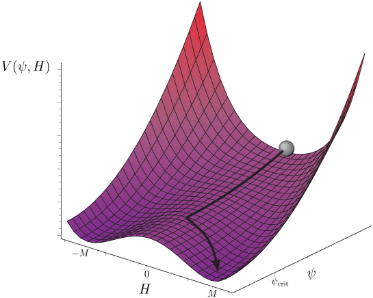
This is a smart way to achieve reheating and it is especially appropriate in the context of intersecting brane models. There, open string tachyons usually do appear after some evolution of the closed string moduli, as discussed in detail in chapter 2.1.6, and then could serve as the $H$ field. This also fits in the sense that the tachyons signal a phase transition in string theory [73, 151], namely, the condensation of higher dimensional D-branes into lower dimensional ones or the condensation of two intersecting D-branes into a single one wrapping a non-trivial supersymmetric 3-cycle [110]. These tachyonic scalars are even well suited to serve as Higgs fields and drive the gauge theory spontaneous symmetry breaking mechanisms [58, 57, 102, 60]. As a speculation, this could link the exit from inflation to a phase transition in the gauge sector of the theory, maybe even to the electroweak phase transition itself.

The possibility of a slowly rolling tachyon by itself also has been discussed in some recent work by Sen [152] that has attracted much attention in the context of cosmology [153, 154, 155, 136, 156].

5.2 Tree level scalar potential for the moduli

Generally speaking, there are two different possibilities of which geometric moduli fields could represent the inflaton, this being the closed and open string moduli.

The closed string moduli are related to the background geometry. If one assumes a factorization of the total space into the 4-dimensional Minkowski space and a compact 6-dimensional subspace, as in the intesecting brane model that we have discussed in all this work, the closed string moduli just come from this subspace. Concretely, these are the Kähler moduli $T^{I}$ (2.16), being related to the size of the tori, and the complex structure moduli $U^{I}$ (2.15) that is related to its shape. Furthermore, in the orbifold models there are the twisted moduli, being localized at the fixed point singularities of these orbifolds.

In contrast to this, the open string moduli are related to the concrete locations of the D-branes in the internal space, or in particular the distance of certain parallel D-branes and the Wilson lines of gauge fields along the branes. It has been discussed in several papers [135, 143, 142] if the open string moduli could satisfy the slow-rolling conditions and the result has been that this is possible if one makes the severe simplification to assume that the closed string moduli are frozen. Geometrically speaking, this means that if the background space is fixed and no backreaction on the presence of the branes takes place, then their motion along this space can be very slow for a certain time. After this time, they start approaching each other faster and at a critical distance a tachyon appears to signal their condensation. On the other hand, the dynamics of the entire setting is determined by the fastest rolling field. Therefore, this assumption implies that the closed string moduli have to roll slower than the open string moduli. Otherwise, the space could for instance shrink very quickly and bring the two branes within their critical distance much faster than originally estimated from the simplified analysis with frozen volume. Only in the simplified brane-anti-brane model the closed string moduli have not been ignored completely [143]. Of course, at first sight, an argument in favor of ignoring the closed string moduli can be found: in a brane-anti-brane setting, the tree level tadpoles are proportional to the inverse volume of the transversal space to the branes. These are driving the dynamics of the transverse geometry, so in a large extra dimension scenario [51, 52], the volume is large and consequently, the tadpoles are suppressed. On the other hand, the evolution of the transverse volume under consideration still can be fast on cosmological scales, so the argument is not solid.

Because of this reason, the main concern in the following will be given to the closed string moduli, their stability or slow-roll behavior being a requirement such that slow rolling in the open sting moduli might be possible as well. It has to be distinguished carefully for these considerations between the so-called string frame, being the usual frame in which perturbative string theory is being performed, and the Einstein-frame that usually is taken for general relativity and cosmology. In this second coordinate system, the dilaton has been transformed away via a spacetime Weyl transformation, which seems reasonable as no phenomenological observations of the dilaton have been made so far.

5.2.1 The potential in the string frame

The potential for the closed string moduli in the string frame has been computed already for the $\Omega R$ orientifold, containing D6-branes intersecting at general angles in equation (2.57), in which only the imaginary part of the three complex structure moduli and the dilaton play a role. Therefore, it already occurs at open string tree level, but still is exact in all orders of $\alpha^{\prime}$. Regarding the orbifold models of chapters 3 and 4, the potential for the untwisted moduli is similar, although one has to carefully consider if some of these moduli are fixed by the orbifold projection. If instead, one is interested in intersecting D-branes of type IIA or type 0 string theory, the contribution from the orientifold planes is absent. This implies in type IIA that any net R-R charge due to supersymmetry is absent, but not so in type 0. In this non-supersymmetric string theory the orientifold planes are rather exotic objects that carry charge but no tension.

The dilaton $\phi$ in the potential (2.57) actually is the 4-dimensional dilaton, that here will be denoted as $\phi_{4}$, because the difference to the 10-dimensional dilaton $\phi_{10}$ will be crucial,

(5.18) $$e^{-\phi_{4}}=M_{\text{s}}^{3}\,e^{-\phi_{10}}\prod_{I=1}^{3}\sqrt{R_{x}^{(I)}\,R_{y}^{(I)}},$$

where $M_{\text{s}}$ is the string mass that should be written down explicitly in this context. Only the $A$-torus with $b_{I}=0$ will be discussed here, as the equations then simplify and the qualitative behavior will be similar to the $B$-torus. Then the potential simplifies:

(5.19) $$V_{\text{s}}(\phi_{4},U^{I}_{2})=M_{\text{s}}^{4}\,e^{-\phi_{4}}\,\left(\sum_{a=1}^{k}N_{a}\,\prod_{I=1}^{3}\sqrt{\left(n_{a}^{I}\right)^{2}{1\over U^{I}_{2}}+\left(m_{a}^{I}\,\right)^{2}U^{I}_{2}}-16\,\prod_{I=1}^{3}\sqrt{\frac{1}{U^{I}_{2}}}\right).$$

and the NS-NS-tadpole cancellation conditions can then be expressed by the wrapping numbers

(5.20) $$\sum_{a=1}^{k}{N_{a}\,\prod_{I=1}^{3}{n_{I}^{a}}}-16=\sum_{a=1}^{k}{N_{a}\,n^{a}_{I}m^{a}_{J}m^{a}_{K}}=0\qquad\text{with}\qquad I\neq J\neq K\ .$$

At this point we recall that the potential for the imaginary part of the Kähler structures $T^{I}_{2}=M_{\text{s}}^{2}R_{x}^{(I)}R_{y}^{(I)}$ is flat at tree-level and thus can be neglected at this order. In the following, we will refer to the two quantities $\phi_{4}$ and $U^{I}_{2}$ by the name ’Planck coordinates’. From these considerations this appears to be the natural choice of variables for expressing the string frame leading order potential.

From 4-dimensional ${\cal N}=1$ supersymmetric effective field theories, it is known that only the particular combinations of scalars

(5.21) $\displaystyle s$ $\displaystyle=M_{\text{s}}^{3}\,e^{-\phi_{10}}\,\prod_{I}R_{x}^{(I)}=e^{-\phi_{4}}\prod_{I}\frac{1}{\sqrt{U^{I}_{2}}},$
$\displaystyle u^{I}$ $\displaystyle=M_{\text{s}}^{3}\,e^{-\phi_{10}}\,R_{x}^{(I)}\,R_{y}^{(J)}\,R_{y}^{(K)}=e^{-\phi_{4}}\sqrt{U^{J}_{2}\,U^{K}_{2}\over U^{I}_{2}}$

appear in chiral superfields such that the effective gauge couplings can be expressed as a linear function of these variables [67]. In terms of these ’gauge coordinates’ the string frame scalar potential can be simply expressed as

(5.22) $$V_{\text{s}}(s,u^{I})=M_{\text{s}}^{4}\,\sum_{a=1}^{k}N_{a}\,\Biggl{[}\left(n^{a}_{1}n^{a}_{2}n^{a}_{3}\right)^{2}\,s^{2}+\sum_{I=1}^{3}\left(n^{a}_{I}m^{a}_{J}m^{a}_{K}\right)^{2}\,\left(u^{I}\right)^{2}\\ +\left(m^{a}_{1}m^{a}_{2}m^{a}_{3}\right)^{2}\left({u^{1}u^{2}u^{3}\over s}\right)+\sum_{I=1}^{3}\left(m^{a}_{I}n^{a}_{J}n^{a}_{K}\right)^{2}\,\left({su^{J}u^{K}\over u^{I}}\right)\Biggr{]}^{\frac{1}{2}}-16\,M_{\text{s}}^{4}\,s\ ,$$

where the last term is the contribution from the O6-planes.

5.2.2 The potential in the Einstein frame

We now make the transition to the Einstein frame by performing the Weyl rescaling

(5.23) $$g^{(4),\text{s}}_{\mu\nu}\rightarrow g^{(4),\text{E}}_{\mu\nu}=e^{2\phi_{4}}g^{(4),\text{s}}_{\mu\nu}\ ,$$

which results in the following potential in the Einstein frame:

(5.24) $$V_{\text{E}}(\phi_{4},U^{I})={M^{4}_{\text{Pl}}\over M^{4}_{\text{s}}}\,e^{4\phi_{4}}\,V_{\text{s}}(\phi_{4},U^{I}),$$

or explicitly,

(5.25) $$V_{\text{E}}(s,u^{I})=M_{\text{Pl}}^{4}\,\sum_{a=1}^{k}N_{a}\,\biggl{[}\left(n^{a}_{1}n^{a}_{2}n^{a}_{3}\right)^{2}\,\left({1\over u^{1}u^{2}u^{3}}\right)^{2}\\ +\sum_{I=1}^{3}\left(n^{a}_{I}m^{a}_{J}m^{a}_{K}\right)^{2}\,\left({1\over s\,u^{J}\,u^{K}}\right)^{2}+\left(m^{a}_{1}m^{a}_{2}m^{a}_{3}\right)^{2}\left({1\over(s)^{3}\,u^{1}\,u^{2}\,u^{3}}\right)\\ +\sum_{I=1}^{3}\left(m^{a}_{I}n^{a}_{J}n^{a}_{K}\right)^{2}\,\left({1\over s\,(u^{I})^{3}\,u^{J}\,u^{K}}\right)\biggr{]}^{1\over 2}-16\,M_{\text{Pl}}^{4}\,\left({1\over u^{1}u^{2}u^{3}}\right).$$

The fact, that there is just one fundamental scale in string theory, implies the following relation between the string scale $M_{\text{s}}$ and the Planck scale $M_{\text{Pl}}$

(5.26) $${M_{\text{s}}\over M_{\text{Pl}}}=e^{\phi_{4}}=(s\,u^{1}\,u^{2}\,u^{3})^{-{1/4}}.$$

This means that a running of any single one of the four fields $s,u^{I}$ at fixed $M_{\text{Pl}}$ implies a dynamical evolution of the fundamental string scale $M_{\text{s}}$.

After a dimensional reduction down to four dimensions, rewriting in terms of the 4-dimensional dilaton and the appropriate Weyl rescaling, the kinetic terms for the scalar fields have the form

(5.27) $$S_{\text{kin}}=M_{\text{Pl}}^{2}\int d^{4}x\,\left[-(\partial^{\mu}\phi_{4})(\partial_{\mu}\phi_{4})-{1\over 4}\sum_{I=1}^{3}{(\partial^{\mu}\log U^{I})(\partial_{\mu}\log U^{I})}\right]\ ,$$

being explicitly calculated in appendix F. In terms of the ’gauge coordinates’ this reads as

(5.28) $$S_{\text{kin}}=M_{\text{Pl}}^{2}\int d^{4}x\,{1\over 4}\,\left[-(\partial^{\mu}\log s)(\partial_{\mu}\log s)-\sum_{I=1}^{3}{(\partial^{\mu}\log u^{I})(\partial_{\mu}\log u^{I})}\right].$$

Besides the transformation into the Einstein frame, these kinetic terms have to be canonically normalized to be comparable to standard cosmological results. The fields $s,u^{I}$ have a logarithmic derivative in (5.27) and (5.28). Therefore, the correctly normalized fields $\tilde{s},\tilde{u}^{I}$ are defined by

(5.29) $${s}=e^{\sqrt{2}{\tilde{s}/M_{\text{Pl}}}}\quad\text{and}\qquad{u}^{I}=e^{\sqrt{2}{\tilde{u}^{I}/M_{\text{Pl}}}}.$$

5.3 Inflation from dilaton and complex structure

A crucial assumption that has been adopted throughout the whole work is that it is possible to work within perturbative string theory. This implies that the 10-dimensional string coupling has to be small and, as it is nothing but the expectation value of the 10-dimensional dilaton, $e^{\phi_{10}}\ll 1$. Another assumption that has to be made for convenience is that numbers of stacks $N_{a}$, and the wrapping numbers $n_{I}^{a}$ and $m_{I}^{a}$ are not extremely large. This seems unproblematic, as very large numbers would result in an unacceptable particle spectrum anyway. But compared to the former work of Burgess et al.[143], we do not have to impose that the internal radii are small compared to the string scale, as our potential is exact to all orders of $\alpha^{\prime}$.

As mentioned in the introduction, the most important constraint are the slow-rolling conditions (5.1), which in the Einstein frame for the two fields $s$ and $u^{I}$ correspond to

(5.30) $$\epsilon={M_{\text{Pl}}^{2}\over 2}\left({V_{\text{E}}^{\prime}(s,u^{I})\over V_{\text{E}}(s,u^{I})}\right)^{2}\ll 1,\qquad\eta=M_{\text{Pl}}^{2}{V_{\text{E}}^{\prime\prime}(s,u^{I})\over V_{\text{E}}(s,u^{I})}\ll 1\ .$$

The derivatives of $V(s,u^{I})$ have to be taken with respect to the canonically normalized fields (5.29). Instead of this set of coordinates, one could as well try to satisfy the slow-rolling conditions using the two fields $\phi_{4}$ and $U^{I}$. At first sight, it seems to be irrelevant which set of coordinates is beeing used as the physical result should not depend on this. But here, the situation is different, as we shall see that inflation is not possible if none of the four moduli are assumed to be frozen. But this freezing then distinguishes among different physical situations: for the set $(s,u^{I})$, due to (5.26), the string scale is always forced to change during inflation if not all moduli are being frozen at the same time. In contrast to this, for the set $(\phi_{4},U^{I})$, the string scale can be made constant by just freezing $\phi_{4}$.

In the following, we will discuss inflation in both coordinate systems, as it is unclear which of these two physical situations is the right one.

5.3.1 Discussion for the coordinates $(s,u^{I})$

According to [143], the coordinates $(s,u^{I})$ are the natural coordinates if one assumes ${\cal N}=1$ supersymmetric dynamics at some higher energy scale. But one has to be careful, as this assumes that there occurs a spontaneous breaking of supersymmetry which can be achieved via a continuous deformation of the theory. Indeed, the vanishing of the supertrace Str$({\cal M}^{2})=0$ in the open string spectrum of toroidal type I intersecting brane world models suggests a spontaneous supersymmetry breaking [58]. On the other hand, the potential $V_{\text{E}}(s,u^{I})$ is not generally of the type which can occur as the scalar potential in a supersymmetric theory. But this means that the only possibility to make the transition would be a discontinuous phase transition, separating the supersymmetric vacuum from the non-supersymmetric theory. This theory then will be non-supersymmetric at all scales for a given set of winding numbers.

It has to be mentioned that under special circumstances, also a continuous phase transition is possible: in a supersymmetric theory, the scalar potential should have the form of a D-term potential. For certain choices of the complex structure moduli, this indeed can be achieved, as being described in [67]. The spontaneous supersymmetry breaking then in a ${\cal N}=1$ supersymmetric theory occurs by adding a Fayet-Iliopoulos term, that is supposed to be the low-energy manifestation of a small change of the complex structure as described in chapter 4.

In our case, such a continuous deformation cannot be guaranteed in general, such that it remains somehow doubtful why $(s,u^{I})$ should be the right variables.

It is a first, somehow disappointing observation from the potential (5.25) that slow rolling definitely is impossible, if not 3 of the parameters $s$ and $u^{I}$ are frozen at the same time. The reason is that the fast rolling scalars destabilize the background before slow-rolling in the other moduli can become relevant on a cosmological scale. This result is almost trivial from a mathematical point of view. Qualitatively, the potential looks like a four-dimensional generalization of a similar potential as shown in figure 5.3. At any point, there always does exist a direction in which the potential is constant, just simply the contour line $V=\text{const}$. On the other hand, it is a non-trivial question if these lines of constant $V$ do correspond or are at least close to certain specific variables like $s$ or $u_{I}$.

Therefore, we will now discuss in analogy to [143] what happens if three moduli are getting frozen ’by hand’. In doing this, we will only discuss the generic situation, neglecting very specific choices of the wrapping numbers or very special regions in parameter space where new features generally might appear.

Inflation in $s$, all $u_{I}$ frozen

For this case, the scalar potential for only the D-branes has the schematic form:

(5.31) $$V_{\text{E}}^{\rm D6}=M_{\text{Pl}}^{4}\sum_{a=1}^{k}N_{a}\,\sqrt{\alpha_{a}+{\beta_{a}\over s^{2}}+{\gamma_{a}\over s}+{\delta_{a}\over s^{3}}},$$

where the coefficients can be read off from (5.25) and involve the fixed scalars $u^{I}$ and some numbers of order one. Due to the appearing squares, $\alpha_{a}>0$. For large values of $s$, we have

(5.32) $$V_{\text{E}}^{\rm D6}=M_{Pl}^{4}\left[\left(\sum_{a}N_{a}\,\sqrt{\alpha_{a}}\right)+{1\over 2}\left(\sum_{a}N_{a}\,{\gamma_{a}\over\sqrt{\alpha_{a}}}\right){1\over s}+\ \cdots\right]\qquad\text{for}\ s\gg\ 1\ .$$

The orientifold planes contribute

(5.33) $$V_{\text{E}}^{\rm O6}=-M_{\text{Pl}}^{4}\,16\left[\prod_{I=1}^{3}u^{I}\right]^{-1}.$$

to the potential. We have to distinguish between two cases:

  1. 1.

    all $\prod_{I}n_{a}^{I}$ positive:
    If we choose all wrapping numbers $\prod_{I}n_{a}^{I}$ to be positive, then the constant term in the D-brane contribution cancels precisely against the O6-planes contribution due to the R-R tadpole cancellation conditions. In this case, one simply gets $V\sim 1/s$, which implies $V^{\prime}\sim V$, with a constant of proportionality of order one 111The derivative of course has to be taken with respect to the canonically normalized field $\tilde{s}$. and $s$ consequently does not show slow-rolling behavior.

  2. 2.

    some $\prod_{I}n_{a}^{I}$ negative:
    If instead some of the $\prod_{I}n_{a}^{I}$ are negative, then the potential takes the form

    (5.34) $$V_{\text{E}}=V_{\text{E}}^{\rm D6}+V_{\text{E}}^{\rm O6}=M_{\text{Pl}}^{4}\left(A+B\,e^{-\sqrt{2}{\tilde{s}/M_{\text{Pl}}}}+\ \cdots\right),$$

    The slow rolling parameters then read

    (5.35) $$\epsilon={B^{2}\over A^{2}}{1\over s^{2}},\quad\quad\eta={2B\over A}{1\over s}\ ,$$

    meaning that $\eta\ll 1$ directly implies $\epsilon\ll 1$. If one inserts the explicit expressions for $\alpha_{a}$ and $\gamma_{a}$, one gets

    (5.36) $$\eta=\sum_{I}\zeta_{I}{u^{J}\,u^{K}\over u^{I}\,s}=\sum_{I}{\zeta_{I}\over\left(U^{I}\right)^{2}}\ ,$$

    If all complex structure moduli satisfy $U^{I}\gg 1$ with their relative ratios fixed, then $s$ is slow rolling. This is self-consistent with the assumption $s\gg 1$, as it is evident from the definition (5.21). So for the given assumptions, $s$ is a reasonable inflaton candidate. One interesting observation for $B>0$ is that the length of the string in this scenario also inflates.

In type II or type 0 string theory, the distinction between the two cases does not apply as no negative orientifold contribution appears in the potential, the potential generally is of the second form (5.34).222Actually, this potential is identical to the one in [143]. The configuration of D$9$- and D$5$-branes in this paper is just a very specific choice of D9-branes with magnetic flux, or more precisely, infinite magnetic flux for a D5-brane. This is the T-dual situation of what is studied here.

Inflation in one $u_{i}$, $s$ and other $u_{I}$ frozen

If one freezes $s$ together with all but one $u_{I}$, one again gets a potential of the form (5.34) in a $1/u^{I}$ expansion. Here, the constant term $A$ never vanishes, not even in type I models, so that the slow-rolling parameter $\eta$ always can be written as

(5.37) $$\eta=\zeta_{1}{u^{J}\,u^{k}\over u^{I}\,s}+\zeta_{2}{u^{J}\,s\over u^{I}\,u^{K}}+\zeta_{3}{u^{K}\,s\over u^{I}\,u^{J}}={\zeta_{1}\over\left(U^{I}\right)^{2}}+\zeta_{2}\left(U^{J}\right)^{2}+\zeta_{3}\left(U^{K}\right)^{2},$$

with all $\zeta_{i}$ of order one. Slow rolling is possible if one requires $U^{I}\gg 1$ and $U^{J},U^{K}\ll 1$, again being self-consistent with the assumption $u^{I}\gg 1$. The constant $A$ is positive, but now the constant $B$ generally can become negative in type I theory, as the orientifold planes contribute as well. In case $B$ is negative, the evolution leads towards smaller values of $u^{I}$ until the slow-rolling condition is no longer satisfied or open string tachyons do appear.

Phenomenological Discussion

In this section, we are going to look at several phenomenological questions that follow the first step of fulfilling the slow-rolling conditions.

  1. 1.

    Inflationary exit scenario
    In the case of $s$-inflation, we had to require $A>0$ and $B>0$ for slow-rolling, so it follows that $\eta>0$ in (5.35) and one faces a positive cosmological constant. Hence $s$ rolls towards larger values, meaning deeper into the slow-rolling region. This means that the naive picture from reheating that at some point the slow-rolling conditions are not fulfilled anymore, does not apply. But there still is another possibility: depending on the angle in between the D-branes, the open string sector can have tachyons, localized at the intersection locus, see for instance equation (3.34). For fixed wrapping numbers $n_{I}$ and $m_{I}$ of the two branes $a$ and $b$, the angle only depends on the complex structure moduli:

    (5.38) $$\theta^{I}={1\over\pi}\,\arctan\left({\left({m_{I}^{b}\over n_{I}^{b}}+{m_{I}^{a}\over n_{I}^{a}}\right)U^{I}\over 1+\left({m_{I}^{a}\,m_{I}^{b}\over n_{I}^{a}\,n_{I}^{b}}\right)\,\left(U^{I}\right)^{2}}\right),$$

    The mass of the lowest bosonic mode is given by

    (5.39) $$M^{2}_{\text{scal}}={1\over 2}\sum_{I=1}^{3}\theta^{I}-{\rm max}\{\theta^{I}:I=1,2,3\},$$

    where one has to assume that $0<\theta^{I}<1/2$, such that this equation is correct. Tachyons do appear, if this squared mass becomes negative, and this triggers the decay of the intersecting brane configuration to different ones, finally to a stable one. So it might be possible that $s(U^{I},\phi_{4})$ first rolls slowly and then, depending on the behavior of the complex structure moduli $U^{I}$, suddenly tachyon condensation is triggered off, leading to a phase transition. If this phase transition is understood to be a cosmic phase transition, then this realizes the hybrid inflation scenario.

    The decay process itself can be understood via boundary string field theory, not by simple perturbative string theory [151, 157, 158, 159]. Nevertheless, the suggestion has been given (and treated in more detail within chapter 3) that the tachyon might act as a Higgs field in the effective gauge theory, based on the simple observation that the tachyon being localized at the brane intersection, carries a bifundamental representation of the unitary gauge groups of the two stacks. This would link the cosmic phase transition with a spontaneous breaking of gauge symmetry.

    In order to better understand the appearing of tachyons, we should take a look at figure 5.2.

    Refer to caption
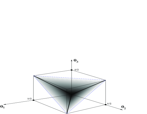
    Figure 5.2: The appearance of tachyons.

    .

    Within the interior of the shaded cone (with edges given by the bold diagonal lines), no tachyons do appear. The system preserves ${\cal N}=1$ supersymmetry on the shaded faces of the cone and ${\cal N}=2$ supersymmetry on the edges. The origin corresponds to parallel branes which preserve the maximal ${\cal N}=4$ supersymmetry. During $s$-inflation the background geometry is driven towards larger values of all three complex structures $U^{I}$ but with their ratios fixed. Using (5.38), we conclude that if none of the two D6-branes is parallel to the $X^{I}$-axis, i.e. $m_{a}^{I}\not=0$ for $a=1,2$, then the intersection angle $\theta^{I}$ is driven to 00. If in fact any one of the two is parallel to the $X^{I}$-axis, then $\theta^{I}$ goes to $1/2$. To summarize, up to permutations we have the following four possible endpoints of the flow

    (5.40) $\displaystyle(\theta^{1},\theta^{2},\theta^{3})$ $\displaystyle\to(0,0,0),$ $\displaystyle{\cal N}=4\ {\rm SUSY,\ no\ tachyons}$
    $\displaystyle(\theta^{1},\theta^{2},\theta^{3})$ $\displaystyle\to(0,1/2,1/2),$ $\displaystyle{\cal N}=2\ {\rm SUSY,\ no\ tachyons}$
    $\displaystyle(\theta^{1},\theta^{2},\theta^{3})$ $\displaystyle\to(0,0,1/2),$ $\displaystyle{\cal N}=0\ {\rm SUSY,\ tachyons}$
    $\displaystyle(\theta^{1},\theta^{2},\theta^{3})$ $\displaystyle\to(1/2,1/2,1/2),$ $\displaystyle{\cal N}=0\ {\rm SUSY,\ no\ tachyons}.$

    This classification actually leaves out the fact that the points that the parameters are driven to cannot be reached within a given set of winding numbers for any finite value of $U^{I}$. For instance in the first case, two branes may approach vanishing intersection angles very closely, but only if their $(n^{a}_{I},m^{a}_{I})$ were proportional, they could become parallel. Thus, there may occur a situation where a set of branes evolves towards an ${\cal N}=4$ supersymmetric setting dynamically, approaching it arbitrarily well, but never reaching it without tachyon condensation. In fact, tachyons can then no longer be excluded for such a brane setting of the first type, as with three very small relative angles, the mass of the NS ground state may still become negative. But one thing clearly can be deduced: Whenever the model contains two intersecting D-branes, where one of the D-branes is parallel to exactly one of the $X^{I}$-axes, the system evolves to a region where tachyons do appear. Unfortunately, it is difficult to determine in general the precise end-point of inflation, i.e. the point where the model crosses one of the faces in figure 5.2.

  2. 2.

    Number of e-foldings, density perturbations and spectral index
    As discussed in chapter 5.1 in detail, inflation must last for a long enough time, or more precisely, for 60 e-foldings, see (5.12). This number can be easily calculated if one makes the simplifying assumption that the potential $V_{\text{E}}$ stays approximately constant during inflation at a value $V_{\text{inf}}$ and one obtains the following criterion:

    (5.41) $$N=-\int_{\tilde{s}_{\text{I}}}^{\tilde{s}_{\text{R}}}d\tilde{s}{1\over M_{\text{Pl}}^{2}}\,{V_{\text{E}}\over V_{\text{E}}^{\prime}}\simeq{A\over 2B}\,(s_{\text{R}}-s_{\text{I}})\simeq 60-\log\left({10^{16}\ {\rm GeV}\over V_{\text{inf}}^{1/4}}\right)\ .$$

    In this equation, the index I refers to the start and the index R to the end of inflation. The magnitude of the primordial density fluctuations (5.14) also can be calculated:

    (5.42) $$\delta_{H}\sim{1\over 5\sqrt{3}\pi}\left({V_{\text{E}}^{3/2}\over M^{3}_{\text{Pl}}\,V_{\text{E}}^{\prime}}\right)\simeq{1\over 5\sqrt{6}\pi}\left({A^{3/2}s_{\text{I}}\over B}\right),$$

    As mentioned earlier, from COBE observations one knows that it should be of the size $\delta_{H}=1.91\times 10^{-5}$. The spectral index (5.15) is calculable as well, it is given by

    (5.43) $$n-1=-6\epsilon_{h}+2\eta_{h}\simeq 2\eta_{h}\simeq{4B\over As_{\text{I}}}\ ,$$

    which has to match the Maxima and Boomerang bounds (5.16).

    For $s$-inflation, one has $A,B>0$ such that $s_{e}\gg s_{h}$, which then implies $N=\eta_{e}^{-1}$. But is impossible to make any more detailed prediction, if $s_{e}$ and $s_{h}$ are unknown.

    For $u^{I}$-inflation, one instead assumes $u^{I}_{I}\gg u^{I}_{R}$ and using $u_{\text{I}}^{I}=-2\,B\,N/A$, it is possible to express the density fluctuations and the spectral index in terms of $N$ and $A$ only:

    (5.44) $$\delta_{H}\simeq{2\over 5\sqrt{6}\pi}{A^{1/2}N},\qquad n-1=-{2\over N}.$$

    As $n$ by Boomerang and Maxima is bounded in between $0.8\leq n\leq 1.2$, one gets a direct the prediction for $A\leq 0.45\times 10^{-10}$ in this case.

5.3.2 Discussion for the coordinates $(\phi_{4},U^{I})$

The potential in the string frame for the coordinates $(\phi_{4},U^{I})$ is given by (5.19). It can be immediately noticed that for $\phi_{4}$ slow-rolling is not possible. On the other hand, for $\phi_{4}$ and two complex structure moduli $U^{I}$ frozen, depending on the the specific winding numbers (and assuming non-trivial intersection angles), the potential is of the type

(5.45) $$V_{\text{E}}(U^{I})=M_{\text{Pl}}^{4}\,{A\,\sqrt{U^{I}}}\qquad\text{or}\qquad V_{\text{E}}(U^{I})=M_{\text{Pl}}^{4}\,{A\over\sqrt{U^{I}}}\ ,$$

for $U^{I}\gg 1$, which in both cases does not fulfil the slow-rolling conditions. It is schematically shown in figure 5.3.
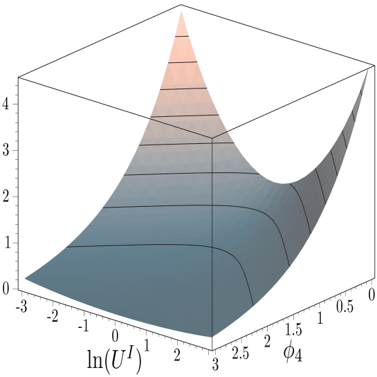
Refer to caption
Figure 5.3: The schematic scalar potential for the coordinates $(\phi_{4},U^{I})$.

The result for the case $U^{I}\ll 1$ is similar, so the only possibility would be near local minima of the potential, that have not been found so far: for all studied examples, $\epsilon\ll 1$ near an extremum, but then $\eta=\mathcal{O}(1)$, although no general proof does exist. Concluding this section, it can be stated that slow rolling seems to be impossible for the choice of coordinates $\phi_{4}$ and $U^{I}$.

5.4 Inflation from the Kähler structure

In the previous section, we have discussed the possibility to achieve slow-rolling for any one of the fields $\phi_{4}$ or $U^{I}$. We have seen that it does not seem to be possible; even more, the only chance to avoid fast rolling is to freeze the complex structures $U^{I}$, while the general stabilization of the dilaton remains an open problem. The complex structure can be frozen by orbifolding, as shown in chapter 3. The are also other possibilities: in type 0’ backgrounds, the complex structures are getting dynamically frozen at values of order one [126], the same is true in type I models with some negative wrapping numbers. A recent example for type IIA orientifold models on Calabi-Yau spaces is given in [160]. There, a three-form G-flux has been turned on, and the freezing of complex structures takes place by means of a F-term scalar potential[88]. Actually, a stabilization of the complex dilaton takes place as well, but one has to keep in mind that this statement is only valid in leading order in string perturbation theory, as $\alpha^{\prime}$ corrections to the Kähler potential may alter the F-term potential. Although it is assumed that this alteration still leaves the dilaton constant, the fact that the D-branes with G-flux and the orientifold planes do not chancel their R-R charges locally, or in other words, D-branes and orientifold planes do not lie on top of each other, invalidates the assumption.

In this section, the assumption will be made that all complex structure moduli $U^{I}$ will be frozen by any such mechanism and the leading order potential for the Kähler moduli will be studied. As the dilaton is not frozen, the tree level potential in the Einstein frame is then given by

(5.46) $$V_{\text{E}}^{\text{tree}}=M_{\text{Pl}}^{4}\,\ C\,\ e^{3\phi_{4}},$$

where $C$ is a constant of order one. A non-trivial dependence of the potential on the Kähler moduli at the earliest arises at one-loop level. If the closed string sector preserves supersymmetry, the torus and Klein-bottle amplitude vanish, because the R-R and NS-NS tadpoles are similar. The remaining cylinder and Möbius strip amplitudes for a non-vanishing angle on a certain 2-torus do depend on its Kähler modulus through the lattice contributions in non-supersymmetric open string sectors. These Kaluza-Klein and winding contributions can also depend on open string moduli, being the distance $x$ between the branes and their relative Wilson line $y$. The Hamiltonian for these modes on one 2-torus is given by

(5.47) $$\mathcal{H}_{\text{lattice, op.}}=\sum_{r,s}\frac{\left|(r+x_{I})+(s+y_{I})T^{I}\right|^{2}}{T^{I}_{2}}\frac{U^{I}_{2}}{|n_{I}+m_{I}U^{I}|^{2}}\ ,$$

which is a generalization of (D.16). More precisely, $0\leq y_{I}\leq 1$ denotes the relative transversal distance between the two D-branes and $0\leq x_{I}\leq 1$ the relative Wilson line along the longitudinal direction of the two D-branes on the specific 2-torus. The full potential can then be understood as a function on $T^{I}$, $x_{I}$ and $y_{I}$.

For simplicity, we will now restrict to the case of two stacks of branes that intersect on two tori but are parallel on the remaining one. Furthermore, we assume that the branes are not parallel to any one of the O6-planes in order to break supersymmetry. Then, the only relevant amplitude at the one-loop level is given by the cylinder diagram for open strings stretching between the two stacks. The potential up to one-loop order is given by

(5.48) $$V_{\text{E}}(T,x,y)=M_{\text{Pl}}\,M_{\text{s}}^{3}\,C_{0}-M_{\text{s}}^{4}\,C_{1}\,-{\cal A}_{ab}(T,x,y)+\ldots\ ,$$

where the first two terms stand for all constant contributions that are independent of $T$,$x$ and $y$. For our simple case, we have just a dependence of ${\cal A}_{ab}$ on one $T^{I}\equiv T$. The three variables are related to the canonical normalized open string moduli by

(5.49) $$Y^{2}={1\over M_{\text{s}}^{2}}\,\Delta\,T\,y^{2},\qquad X^{2}={1\over M_{\text{s}}^{2}}\,{\Delta\over T}\,x^{2}\ ,$$

where $\Delta$ is a constant of order one, depending on the specific wrapping numbers of the D-branes and the choice of model $b=0$ or $b=1/2$. From (C.25) and (C.36), we directly obtain the complete cylinder loop channel amplitude

(5.50) $${\cal A}_{ab}(T,x,y)={M_{\text{Pl}}^{4}\over(8\pi^{2})^{2}}\,e^{4\phi_{4}}\,N_{a}\,N_{b}\,I_{ab}\int_{0}^{\infty}{dt\over t^{3}}\,\left(\sum_{r,s\in\mathbb{Z}}e^{-2\pi t\,\Delta\,\left[{(r+x)^{2}/T}+T(s+y)^{2}\right]}\right)\\ \cdot\left(\frac{\vartheta\bigg{[}{\begin{array}[]{*{20}c}0\\ 0\\ \end{array}}\bigg{]}^{2}\vartheta\bigg{[}{\begin{array}[]{*{20}c}\kappa_{1}\\ 0\\ \end{array}}\bigg{]}\vartheta\bigg{[}{\begin{array}[]{*{20}c}\kappa_{2}\\ 0\\ \end{array}}\bigg{]}-e^{-\pi i(\kappa_{1}+\kappa_{2})}\,\vartheta\bigg{[}{\begin{array}[]{*{20}c}0\\ {1\over 2}\\ \end{array}}\bigg{]}^{2}\vartheta\bigg{[}{\begin{array}[]{*{20}c}\kappa_{1}\\ {1\over 2}\\ \end{array}}\bigg{]}\vartheta\bigg{[}{\begin{array}[]{*{20}c}\kappa_{2}\\ {1\over 2}\\ \end{array}}\bigg{]}}{\eta^{6}\,\vartheta\bigg{[}{\begin{array}[]{*{20}c}\kappa_{1}+{1\over 2}\\ {1\over 2}\\ \end{array}}\bigg{]}\vartheta\bigg{[}{\begin{array}[]{*{20}c}\kappa_{2}+{1\over 2}\\ {1\over 2}\\ \end{array}}\bigg{]}e^{-\pi i(\kappa_{1}+\kappa_{2}+1)}}\right.\\ \left.-\frac{\vartheta\bigg{[}{\begin{array}[]{*{20}c}{1\over 2}\\ 0\\ \end{array}}\bigg{]}^{2}\vartheta\bigg{[}{\begin{array}[]{*{20}c}\kappa_{1}+{1\over 2}\\ 0\\ \end{array}}\bigg{]}\vartheta\bigg{[}{\begin{array}[]{*{20}c}\kappa_{2}+{1\over 2}\\ 0\\ \end{array}}\bigg{]}}{\eta^{6}\,\vartheta\bigg{[}{\begin{array}[]{*{20}c}\kappa_{1}+{1\over 2}\\ {1\over 2}\\ \end{array}}\bigg{]}\vartheta\bigg{[}{\begin{array}[]{*{20}c}\kappa_{2}+{1\over 2}\\ {1\over 2}\\ \end{array}}\bigg{]}e^{-\pi i(\kappa_{1}+\kappa_{2}+1)}}\right).$$

The argument of the $\vartheta$-functions are given by $q=\exp(-2\pi t)$ and for the NS-sector ground state energy, one obtains

(5.51) $$M^{2}_{\text{scal}}=\left[\left(\Delta{x^{2}\over T}+\Delta\,T\,y^{2}\right)+{1\over 2}\left(\kappa_{1}+\kappa_{2}\right)-{\rm max}\{\kappa_{I}:I=1,2\}\right]\ \text{for}\ 0<\kappa_{I}<1/2\ .$$

The modular transformation to the tree channel via $l=1/(2t)$ leads to

(5.52) $$\widetilde{{\cal A}}_{ab}(T,x,y)={M_{\text{Pl}}^{4}\over(8\pi^{2})^{2}}\,e^{4\phi_{4}}\,N_{a}\,N_{b}\,I_{ab}\int_{0}^{\infty}{dl}\,\left({1\over\Delta}\sum_{r,s\in\mathbb{Z}}e^{-\frac{\pi l}{\Delta}\,\left[{T\,r^{2}}+\frac{s^{2}}{T}\right]}\,e^{-2\pi i(r\,x+s\,y)}\right)\\ \cdot\left(\frac{\vartheta\bigg{[}{\begin{array}[]{*{20}c}0\\ 0\\ \end{array}}\bigg{]}^{2}\vartheta\bigg{[}{\begin{array}[]{*{20}c}0\\ \kappa_{1}\\ \end{array}}\bigg{]}\vartheta\bigg{[}{\begin{array}[]{*{20}c}0\\ \kappa_{2}\\ \end{array}}\bigg{]}-\vartheta\bigg{[}{\begin{array}[]{*{20}c}0\\ {1\over 2}\\ \end{array}}\bigg{]}^{2}\vartheta\bigg{[}{\begin{array}[]{*{20}c}0\\ \kappa_{1}+{1\over 2}\\ \end{array}}\bigg{]}\vartheta\bigg{[}{\begin{array}[]{*{20}c}0\\ \kappa_{2}+{1\over 2}\\ \end{array}}\bigg{]}}{\eta^{6}\,\vartheta\bigg{[}{\begin{array}[]{*{20}c}{1\over 2}\\ \kappa_{1}+{1\over 2}\\ \end{array}}\bigg{]}\vartheta\bigg{[}{\begin{array}[]{*{20}c}{1\over 2}\\ \kappa_{2}+{1\over 2}\\ \end{array}}\bigg{]}}\right.\\ \left.-\frac{\vartheta\bigg{[}{\begin{array}[]{*{20}c}{1\over 2}\\ 0\\ \end{array}}\bigg{]}^{2}\vartheta\bigg{[}{\begin{array}[]{*{20}c}{1\over 2}\\ \kappa_{1}\\ \end{array}}\bigg{]}\vartheta\bigg{[}{\begin{array}[]{*{20}c}{1\over 2}\\ \kappa_{2}\\ \end{array}}\bigg{]}}{\eta^{6}\,\vartheta\bigg{[}{\begin{array}[]{*{20}c}{1\over 2}\\ \kappa_{1}+{1\over 2}\\ \end{array}}\bigg{]}\vartheta\bigg{[}{\begin{array}[]{*{20}c}{1\over 2}\\ \kappa_{2}+{1\over 2}\\ \end{array}}\bigg{]}}\right),$$

where the argument of the $\vartheta$-functions is $q=\exp(-4\pi l)$. This amplitude contains divergencies, coming from the uncancelled NS-tadpoles for the non-supersymmetric vacua, we are interested in. In order to make cosmological calculations, one has to regularize (5.52) by subtracting the divergencies

(5.53) $$\widetilde{{\cal A}}_{ab}^{\rm reg}(T,x,y)=\widetilde{{\cal A}}_{ab}(T,x,y)-\widetilde{K}_{ab},$$

which are just given by

(5.54) $$\widetilde{K}_{ab}={M_{\text{s}}^{4}\over(8\pi^{2})^{2}}\,N_{a}\,N_{b}\,I_{ab}\int_{0}^{\infty}{dl}\,{4\over\Delta}\,{\sin^{2}\left({\pi(\kappa_{1}+\kappa_{2})\over 2}\right)\,\sin^{2}\left({\pi(\kappa_{1}-\kappa_{2})\over 2}\right)\over\sin(\pi\kappa_{1})\,\sin(\pi\kappa_{2})}\ .$$

The first observation we can make is that the Kähler modulus gets stabilized dynamically, the argument being as follows: if $x=y$, then (5.47) is invariant under T-duality, exchanging $x$ and $y$. Therefore, there must be at least a local extremum around the self-dual point $T_{\text{sd}}=1$, fixing the internal radii at values of order of the string scale. In figure 5.4, a numerically calculated example of the potential (5.48) is shown.

Assuming $T$ is frozen, then still the open string moduli $x=y$ could show a slow-rolling behavior if $x=y$ is dynamically stable (what indeed is the case, see the left plot in figure 5.4). In a similar situation, such a result indeed has been found [135] for $T\gg 1$ in the neighborhood of the instable antipodal point. In this example, the second derivative $V^{\prime\prime}$ of the potential vanishes at the antipodal point, therefore both $\epsilon$ and $\eta$ become small, what is sufficient for slow-rolling.

It is an important question, if this statement stays true when T approaches its true minimum at $T=1$, where also massive contributions contribute to the force between the two D-branes. In order to clarify this point, we are going to expand the annulus amplitude (5.52) in $q$. Taking the zeroth order term $q^{0}$ in the $\vartheta$- and $\eta$-functions, but summing over all Kaluza-Klein and winding modes, means that one has to evaluate the integral

(5.55) $$\int_{0}^{\infty}dl\left[\left(1+2\sum_{r\geq 1}e^{-\frac{\pi l}{\Delta}\,{T\,r^{2}}}\cos(2\pi rx)\right)\left(1+2\sum_{s\geq 1}e^{-\frac{\pi l}{\Delta}\,{{s^{2}\over T}}}\cos(2\pi sy)\right)-1\right].$$

After expanding the result around the ’symmetric antipodal’ point, by using $x=1/2-\o x$, $y=1/2-\o y$, we find that the linear and quadratic terms in the fluctuations $\o x$ and $\o y$ precisely vanish, confirming the large distance result of [135]. On the other hand, we have found that out minimum in $T$ is at distances of the order of the string scale, $T=1$. If one now also takes higher order terms like $q^{1}$ into account, one finds that although the linear terms in $\o x,\ \o y$ still vanish, the quadratic terms do not. This destroys the slow-rolling property, because $\eta$ is not small any longer. The same result has been found in the numerical integration of the complete amplitude (5.53), where also numerically the first and second field derivative have been calculated. The potential is shown for a typical example in figure 5.4.

Refer to caption
Figure 5.4: The numerically integrated regularized cylinder amplitude for the typical example $\kappa_{1}=1/3$, $\kappa_{2}=-1/3$, $\Delta=\sqrt{3}/14$, where the off-set of the amplitude has been chosen arbitrarily. The left plot shows the dynamical stability of $x=y$ for $T=1$, where the grey area at the bottom indicates the appearance of tachyons when the numerical integration is diverging. The right plot shows the minimum at $T=1$ for $x=y$, slow-rolling is not possible as $V^{\prime\prime}$ is not small.

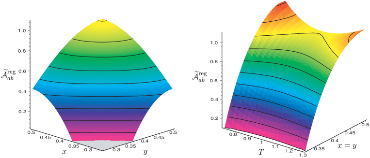
Concluding this section, it can be stated that no slow-rolling properties could be found for the open string moduli $x$ and $y$ near the minimum of the dynamically stabilized Kähler modulus. Consequently, inflation seems to be impossible using any of these moduli fields.

Chapter 6 Conclusions and Outlook

The main concern of this work has been to elaborate on possible phenomenological model building approaches within orientifolded type II string theory containing intersecting D6-branes. This has been done with respect to both particle accelerator physics and cosmology. A particularly important guiding principle has been the issue of stability.

Chapter 2 has provided a detailed survey of the construction principles for these particular models. The string theoretical conformal field theory construction has been discussed in great detail, using the toroidal $\Omega R$ orientifold as an example. The R-R tadpole cancellation condition, being the most important consistency requirement, has been derived for this model. The scalar moduli potential for the toroidal model has been obtained from the NS-NS tadpole for a first time, being of most significance for stability. Indeed, it has been shown that toroidal orientifold models generally suffer from complex structure and dilaton instabilities already at one-loop level.

Furthermore, it has been discussed how to obtain the open and closed string massless spectra, which are essential for low energy model building. The absence of quantum anomalies in spacetime has been addressed, mainly being a consequence from R-R tadpole cancellation for the non-abelian anomalies, and involving a generalized Green-Schwarz mechanism as a string theoretical tool in the case of mixed anomalies. Finally, different gauge breaking mechanisms have been discussed.

In chapter 3, it has been searched for a stable non-supersymmetric standard model. The $\mathbb{Z}_{3}$-orientifold has emerged to be particularly useful in this respect as all complex structures are fixed, therefore ensuring that the background geometry is not driven to the degenerate limit of collapsed 2-tori. Two particular examples containing 3 generations of chiral matter are discussed in detail, a standard-like model with gauge groups $SU(3)\times SU(2)_{L}\times U(1)_{Y}\times U(1)_{B-L}$ and a flipped $SU(5)\times U(1)$ model. The standard-like model shows some deviation from the usual standard model: first, there are right handed neutrinos, this is definitely a strong prediction. Secondly, there exists an additional $B-L$-symmetry which survives as a global symmetry after a discussed gauge breaking mechanism. The additional global symmetry prohibits the standard model Yukawa couplings of the $(u,c,t)$ quarks with electroweak Higgs doublets. As a consequence, the standard mass generation mechanism with fundamental Higgs scalars does not work and a composite Higgs particle has to be incorporated to cure this problem. On the other hand, this model yields a massless hypercharge, being a non-trivial result.

This model is related to the second flipped $SU(5)$ model by an adjoint breaking if the initial $U(3)$ and $U(2)$ stacks of branes are parallel. The flipped $SU(5)$-model yields the GUT result for Weinberg angle $\sin^{2}\theta_{W}=3/8$. Unfortunately, there is a problem with proton decay and gauge coupling unification if the string scale is of the same order as the GUT scale. Therefore, the natural scale for the discussed model appears to be the GUT scale instead of the TeV scale.

Chapter 4 approaches the hierarchy problem by directly constructing a $\mathcal{N}$=1 supersymmetric model. The $\mathbb{Z}_{4}$-orbifold has proved to be a well suited example to do so, intrinsically containing also exceptional cycles from the fixed points. Fractional D-branes, i.e. branes which also wrap around these twisted 3-cycles, are being constructed for the first time explicitly for this type of models. Finally, a three generation Pati-Salam model with gauge groups $SU(4)\times SU(2)\times SU(2)$ is being obtained, involving a brane recombination mechanism. As a consequence, some of the branes are non-flat and non-factorizable and one can only use a description by homology and some tools from effective field theory like quiver diagrams to discuss phenomenological aspects.

In Chapter 5 the question has been discussed if the unstable moduli, which are often unavoidable in non-supersymmetric intersecting brane scenarios, might play the role of the inflaton in cosmology. A candidate field would have to fulfill in particular the slow-rolling condition. Two different possibilities have been discussed, the unstable moduli coming from either the open or closed string sector.

For the closed string moduli, the result was negative if there is no assumed stabilization mechanism for some of the moduli. It has to be distinguished between two different physical situations. First of all, there has been a discussion for the introduced ’gauge coordinates’ which yielded the result that the potential fulfills slow-rolling conditions for both $s$- or $u^{I}$-Inflation if the three remaining moduli are frozen. Then, the scenario of the ’Planck coordinates’ has been discussed in detail. Here, slow-rolling was generally not possible.

For the open string leading order moduli scalar potential, it has been found out that the Kähler moduli are being stabilized dynamically in the discussed type of models, such that they cannot lead to inflation. Also at the antipodal points of the open string moduli, the slow-rolling properties are not fulfilled for small values of the internal radii at the minimum of the potential.

In order to conclude, one can say that intersecting D-branes in type IIA theory are very successful for phenomenological model building and a good alternative to the heterotic string. Nevertheless, some of the most important problems have not been generally solved so far. There is still no string-theoretical realization of the exact matter content of the MSSM. In order to obtain such a model, it might be interesting to extend the ideas of chapter 4 also to $\mathbb{Z}_{6}$ or $\mathbb{Z}_{N}\times\mathbb{Z}_{M}$ orbifolds. This already has been done for the case of $\mathbb{Z}_{4}\times\mathbb{Z}_{2}$ [47]. Furthermore, it would be very interesting to also address the question of gauge coupling unification in these supersymmetric models, a first attempt is given by [49].

Considering more fundamental problems, one has to understand the dynamical mechanism of supersymmetry breaking for these models. Some progress already has been made in [50]. Another great problem is the instability of the dilaton, where one has to think about possible stabilization mechanisms. Tachyon condensation also deserves a better understanding within intersecting D-branes.

As one can see already from these short outlook, there remains a lot to be done in future work.

Appendix A Superstring Coordinates and Hamiltonians

In this chapter, we will give definitions for the superstring coordinates and Hamilton operators that are used in the main text. These are given for light cone quantization, which is generally used in the field of intersecting branes.

In the closed string, the bosonic coordinates in terms of oscillators can be separated into a left and right moving part:

(A.1) $$X^{\mu}(\tau,\sigma)=X_{R}^{\mu}(\tau-\sigma)+X_{L}^{\mu}(\tau+\sigma)\ ,$$

which are given by:

(A.2) $\displaystyle X^{\mu}_{L}(\tau+\sigma)=\frac{x^{\mu}}{2}+\frac{p_{L}^{\mu}}{2}(\tau+\sigma)+\frac{i}{\sqrt{2}}\sum_{n\not=0}{\frac{\alpha^{\mu}_{n}}{n}e^{-in(\tau+\sigma)}}\ ,$
$\displaystyle X^{\mu}_{R}(\tau-\sigma)=\frac{x^{\mu}}{2}+\frac{p_{R}^{\mu}}{2}(\tau-\sigma)+\frac{i}{\sqrt{2}}\sum_{n\not=0}{\frac{\tilde{\alpha}^{\mu}_{n}}{n}e^{-in(\tau-\sigma)}}\ .$

In this equation, $x^{\mu}$ and $p^{\mu}=p_{L}^{\mu}+p_{R}^{\mu}$ are the center of mass position and momentum, respectively. They are given in units of $\alpha^{\prime}$. The same division into left and right movers can be done for the fermionic coordinates:

(A.3) $$\Psi^{\mu}(\tau,\sigma)=\Psi_{R}^{\mu}(\tau-\sigma)+\Psi_{L}^{\mu}(\tau+\sigma)\ ,$$

that are then given by:

(A.4) $\displaystyle\Psi^{\mu}_{L}(\tau+\sigma)=\sum_{r\in\mathbb{Z}+\nu}{\psi_{r}^{\mu}e^{-ir(\tau+\sigma)}}\ ,$
$\displaystyle\Psi^{\mu}_{R}(\tau-\sigma)=\sum_{r\in\mathbb{Z}+\tilde{\nu}}{\tilde{\psi}_{r}^{\mu}e^{-ir(\tau-\sigma)}}\ ,$

where the left and right moving $\nu$ and $\tilde{\nu}$ take the value 00 in the Ramond and $1/2$ in the Neveu-Schwarz sector. This leads to commutation relations of the kind:

$\displaystyle\left[\alpha^{\mu}_{n},\alpha^{\nu}_{m}\right]=\left[\tilde{\alpha}^{\mu}_{n},\tilde{\alpha}^{\nu}_{m}\right]=n\delta_{n+m,0}\,\delta^{\mu\nu}\ ,$
(A.5) $\displaystyle\{\psi_{r}^{\mu},\psi_{s}^{\nu}\}=\{\tilde{\psi}_{r}^{\mu},\tilde{\psi}_{s}^{\nu}\}=\delta_{r+s,0}\,\delta^{\mu\nu}\ ,$
$\displaystyle\left[\alpha^{\mu}_{n},\tilde{\alpha}^{\nu}_{m}\right]=\{\psi_{r}^{\mu},\tilde{\psi}_{s}^{\nu}\}=0\ .$

In the NS-sector, the ground state is unique, whereas in the R-sector, the groundstate is degenerate and carries a representation of the Clifford algebra.

The Hamilton operator of the closed string does not depend on the specific placements of the D-branes, it is a sum of the left and right moving parts and given by:

(A.6) $${\mathcal{H}}_{\text{closed}}=({p^{\mu}})^{2}+\sum_{\mu=1}^{10}{\left(\sum_{n=1}^{\infty}{\left(\alpha_{-n}^{\mu}\alpha_{n}^{\mu}+\tilde{\alpha}_{-n}^{\mu}\tilde{\alpha}_{n}^{\mu}\right)}\right.}\\ \left.+\sum_{r\in\mathbb{Z}+\nu,\ r>0}{\left(r\psi^{\mu}_{-r}\psi^{\mu}_{r}\right)}+\sum_{s\in\mathbb{Z}+\tilde{\nu},\ s>0}{\left(s\tilde{\psi}^{\mu}_{-s}\tilde{\psi}^{\mu}_{s}\right)}\right)+E_{0}^{L}+E_{0}^{R}\ .$$

By way of contrast, the Hamilton operator of the open string does depend on the placement of the D-branes. At this point, it is useful to define complex oscillators on the three compact 2-tori by

(A.7) $$\alpha^{I}=\frac{1}{\sqrt{2}}\left(\alpha^{X_{I}}+i\alpha^{Y_{I}}\right)\ ,\qquad\qquad\alpha^{\bar{I}}=\frac{1}{\sqrt{2}}\left(\alpha^{X_{I}}-i\alpha^{Y_{I}}\right)\ .$$

As an example the Hamiltonian is given for strings that stretch between two certain D6-branes that intersect at an angle of $\kappa={(\varphi_{2}-\varphi_{1})}/{\pi}$:

(A.8) $${\mathcal{H}}_{\text{open}}=\frac{({p^{\mu}})^{2}}{2}+\sum_{\mu=1}^{4}{\left(\sum_{n=1}^{\infty}{\left(\alpha_{-n}^{\mu}\alpha_{n}^{\mu}\right)}+\sum_{r\in\mathbb{Z}+\nu,\ r>0}{\left(r\psi^{\mu}_{-r}\psi^{\mu}_{r}\right)}\right)}\\ +\sum_{I=1}^{3}{\left[\sum_{m\in\mathbb{Z}+\kappa,m>0}{\left(\alpha_{-m}^{I}\alpha_{m}^{\bar{I}}+\alpha_{-m}^{\bar{I}}\alpha_{m}^{I}\right)}+\sum_{s\in\mathbb{Z}+\nu+\kappa,\ s>0}{s\left(\psi^{I}_{-s}\psi^{\bar{I}}_{s}+\psi^{\bar{I}}_{-s}\psi^{I}_{s}\right)}\right]}+E_{0}\ .$$

The zero point energies in light cone gauge can be determined by the following general formulae for in each case one complex particle:

(A.9) $\displaystyle E_{0}^{\text{boson}}=-\frac{1}{12}+\frac{1}{2}\kappa\left(1-\kappa\right)$ $\displaystyle\text{boson with moding }\mathbb{Z}+\kappa\ ,$
$\displaystyle E_{0}^{\text{fermion, R}}=-\frac{1}{24}+\frac{1}{2}\left(\frac{1}{2}-\kappa\right)^{2}$ $\displaystyle\text{R-sector fermion with moding }\mathbb{Z}+\kappa\ ,$
$\displaystyle E_{0}^{\text{fermion, NS}}=-\frac{1}{24}+\frac{1}{2}\kappa^{2}$ $\displaystyle\text{NS-sector fermion with moding }\mathbb{Z}+\kappa\ .$

Appendix B Modular functions

In order to apply the modular transformations, the following equations are important, they are valid for an argument $q=\exp(-2\pi t)$. Many more useful formulas can be found in [161].

(B.1) $$\vartheta\bigg{[}{\begin{array}[]{*{20}c}a\\ b\\ \end{array}}\bigg{]}\left(t\right)=e^{2\pi iab}\ t^{-1/2}\ \vartheta\bigg{[}{\begin{array}[]{*{20}c}b\\ -a\\ \end{array}}\bigg{]}\left(1/t\right)\ ,$$
(B.2) $$\eta(t)=t^{-1/2}\ \eta(1/t)\ .$$

Then there is the Poisson resummation formula

(B.3) $$\sum\limits_{n\in\mathbb{Z}}e^{-\frac{\pi(n-c)^{2}}{t}}=\sqrt{t}\sum\limits_{m\in\mathbb{Z}}e^{2\pi icm}\ e^{-\pi m^{2}t}\ ,$$

from which directly follows:

(B.4) $$\sum\limits_{m\in\mathbb{Z}}e^{-\pi m^{2}t}=t^{-1/2}\sum\limits_{n\in\mathbb{Z}}e^{-{\pi n^{2}}/{t}}\ .$$

For a general argument $q$, the theta functions with characteristics are defined as

(B.5) $$\vartheta\bigg{[}{\begin{array}[]{*{20}c}a\\ b\\ \end{array}}\bigg{]}\left(q\right)=\sum\limits_{n\in\mathbb{Z}}q^{(n+a)^{2}/2}e^{2\pi i(n+a)b}\ ,$$

or in product form:

(B.6) $$\vartheta\bigg{[}{\begin{array}[]{*{20}c}a\\ b\\ \end{array}}\bigg{]}\left(q\right)=e^{2\pi iab}q^{a^{2}/2}\prod\limits_{m=1}^{\infty}\left(1-q^{m}\right)\left(1+e^{2\pi ib}q^{m-1/2+a}\right)\left(1+e^{-2\pi ib}q^{m-1/2-a}\right)\ ,$$

where $a$ has to be chosen within the range $-1/2<a\leq 1/2$. The theta functions have the following important identities:

(B.11) $\displaystyle\vartheta\bigg{[}{\begin{array}[]{*{20}c}a\pm 1\\ b\\ \end{array}}\bigg{]}\left(q\right)=\vartheta\bigg{[}{\begin{array}[]{*{20}c}a\\ b\\ \end{array}}\bigg{]}\left(q\right)\ ,$
(B.16) $\displaystyle\vartheta\bigg{[}{\begin{array}[]{*{20}c}a\\ b\pm 1\\ \end{array}}\bigg{]}\left(q\right)=e^{\pm 2\pi ia}\ \vartheta\bigg{[}{\begin{array}[]{*{20}c}a\\ b\\ \end{array}}\bigg{]}\left(q\right)\ .$

Furthermore, the following product representation is useful:

(B.17) $$\frac{\vartheta\bigg{[}{\begin{array}[]{*{20}c}a\\ b\\ \end{array}}\bigg{]}}{\eta}=e^{2\pi iab}q^{\frac{a^{2}}{2}-\frac{1}{24}}\prod\limits_{m=1}^{\infty}\left(1+e^{2\pi ib}q^{m-1/2+a}\right)\left(1+e^{-2\pi ib}q^{m-1/2-a}\right)\ .$$

Also very important is Jacobi’s abstruse identity:

(B.18) $$\vartheta^{4}\bigg{[}{\begin{array}[]{*{20}c}0\\ 0\\ \end{array}}\bigg{]}\left(q\right)-\vartheta^{4}\bigg{[}{\begin{array}[]{*{20}c}0\\ 1/2\\ \end{array}}\bigg{]}\left(q\right)-\vartheta^{4}\bigg{[}{\begin{array}[]{*{20}c}1/2\\ 0\\ \end{array}}\bigg{]}\left(q\right)=0\ .$$

The Dedekind $\eta$ function in product form is defined as

(B.19) $$\eta(q)=q^{1/24}\prod\limits_{m=1}^{\infty}(1-q^{m})\ .$$

$\eta$ also can be written as a sum:

(B.20) $$\eta(q)=q^{1/24}\left(1+\sum_{n=1}^{\infty}(-1)^{n}\left[q^{n(3n-1)/2}+q^{n(3n+1)/2}\right]\right)\ .$$

Then, there is the useful relation:

(B.21) $$\lim_{\phi\rightarrow 0}\frac{2\sin(\pi\phi)}{\vartheta\bigg{[}{\begin{array}[]{*{20}c}1/2\\ 1/2+\phi\\ \end{array}}\bigg{]}\left(q\right)}=-\frac{1}{\eta^{3}(q)}\ .$$

Appendix C The cylinder amplitude for $\mathbb{Z}+\kappa$ moding

In this section, a simple but general prescription is given, of how to find the correct cylinder amplitude for any sector with a non-trivial moding, without having to quantize the string again from first principles. This can be applied to both branes at non-vanishing angles as to twisted sectors in orbifold theories.

C.1 One complex boson

For $\mathbb{Z}$-moding, the contribution of one complex boson to the trace of the loop channel one loop amplitude is simply given by

(C.1) $$f_{\text{boson, loop}}^{\text{$\mathbb{Z}$-moding}}=\frac{1}{{\eta(q)}^{2}}\ .$$

In a sector with $\mathbb{Z}+\kappa$ moding, two things have to be altered, the first one being the moding within the product representation of the $\eta$-function (B.19)and the second being the zero point energy.

The correct change of the moding within the $\eta$-function is given by

(C.2) $$\eta^{2}\rightarrow q^{\frac{1}{12}}\prod_{n=0}^{\infty}\left(1-q^{n+\kappa}\right)\prod_{m=1}^{\infty}\left(1-q^{m-\kappa}\right)\ .$$

This can be rewritten as

(C.3) $\displaystyle q^{\frac{1}{12}}\prod_{n=0}^{\infty}\left(1-q^{n+\kappa}\right)\prod_{m=1}^{\infty}\left(1-q^{m-\kappa}\right)$
$\displaystyle=q^{\frac{1}{12}}\left(1-q^{\kappa}\right)\prod_{n=1}^{\infty}\left(1+e^{2\pi i\frac{1}{2}}q^{n+\left(\kappa-\frac{1}{2}\right)+\frac{1}{2}}\right)\prod_{m=1}^{\infty}\left(1+e^{-2\pi i\frac{1}{2}}q^{m-\left(\kappa-\frac{1}{2}\right)-\frac{1}{2}}\right)$
(C.6) $\displaystyle=q^{\frac{1}{12}}e^{-\left(\kappa-\frac{1}{2}\right)\pi i}q^{\frac{1}{24}-\frac{\left(\kappa-\frac{1}{2}\right)^{2}}{2}}\frac{\vartheta\bigg{[}{\begin{array}[]{*{20}c}\kappa-1/2\\ 1/2\\ \end{array}}\bigg{]}\left(q\right)}{\eta(q)}$
(C.9) $\displaystyle=e^{-\left(\kappa-\frac{1}{2}\right)\pi i}q^{\frac{\kappa-\kappa^{2}}{2}}\frac{\vartheta\bigg{[}{\begin{array}[]{*{20}c}\kappa-1/2\\ 1/2\\ \end{array}}\bigg{]}\left(q\right)}{\eta(q)}\ .$

As the next step, the zero point energy has to be corrected according to equation (A.9). A check that such a procedure is justified is given by the series expansion of (C.3) that gives a zero point energy $E_{0}=1/12$ which is just the correct one in the case of $\mathbb{Z}$-moding. One has to include by hand the shift

(C.10) $$\Delta E_{0}=\frac{1}{2}\kappa\left(1-\kappa\right)\ ,$$

which finally leads to the following loop channel trace contribution:

(C.11) $$f_{\text{boson, loop}}^{\text{($\mathbb{Z}+\kappa$)-moding}}=e^{\left(\kappa-\frac{1}{2}\right)\pi i}\frac{\eta(q)}{\vartheta\bigg{[}{\begin{array}[]{*{20}c}\kappa-1/2\\ 1/2\\ \end{array}}\bigg{]}\left(q\right)}\ .$$

C.2 One complex fermion

For $\mathbb{Z}$-moding, the contribution of one complex fermion to the trace of the loop channel amplitude is simply given by

(C.12) $$f_{\text{fermion, loop}}^{\text{$\mathbb{Z}$-moding}}=\frac{\vartheta\bigg{[}{\begin{array}[]{*{20}c}a\\ b\\ \end{array}}\bigg{]}\left(q\right)}{\eta(q)},$$

where $a$ and $b$ take the usual values of the type I theory in the R or NS sectors. Changing the moding to $\mathbb{Z}+\kappa$ in the product representation (B.17) simply means

(C.13) $$\frac{\vartheta\bigg{[}{\begin{array}[]{*{20}c}a\\ b\\ \end{array}}\bigg{]}\left(q\right)}{\eta(q)}\rightarrow e^{2\pi iab}q^{\frac{a^{2}}{2}-\frac{1}{24}}\prod\limits_{m=1}^{\infty}\left(1+e^{2\pi ib}q^{m+\kappa-1/2+a}\right)\left(1+e^{-2\pi ib}q^{m-\kappa-1/2-a}\right)\ .$$

In order to rewrite this equation correctly, one has to distinguish between R- and NS-loop channels, which correspond to $a=1/2$ and $a=0$ respectively, the reason being that the product representation is just defined correctly for a first characteristic of the theta function within the range from $-1/2$ to $1/2$.

Starting with the NS-sector, one rewrites (C.13) in the following way:

(C.14) $\displaystyle e^{2\pi iab}q^{\frac{a^{2}}{2}-\frac{1}{24}}\prod\limits_{m=1}^{\infty}\left(1+e^{2\pi ib}q^{m+(a+\kappa)-1/2}\right)\left(1+e^{-2\pi ib}q^{m-(a+\kappa)-1/2}\right)$
(C.19) $\displaystyle=e^{-2\pi ib\kappa}q^{-a^{\prime}\kappa+\frac{\kappa^{2}}{2}}\frac{\vartheta\bigg{[}{\begin{array}[]{*{20}c}a^{\prime}\\ b\\ \end{array}}\bigg{]}\left(q\right)}{\eta(q)}=e^{-2\pi ib\kappa}q^{-\left(a\kappa+\frac{\kappa^{2}}{2}\right)}\frac{\vartheta\bigg{[}{\begin{array}[]{*{20}c}a+\kappa\\ b\\ \end{array}}\bigg{]}\left(q\right)}{\eta(q)}\ ,$

where $a^{\prime}=a+\kappa$. Next, the zero point energy has to be altered according to (A.9), this induces a shift

(C.20) $$\Delta E_{0}=\frac{1}{2}\kappa^{2}\ .$$

Finally, setting $a=0$ leads to the result

(C.21) $$f_{\text{fermion, NS-loop}}^{\text{($\mathbb{Z}+\kappa$)-moding}}=e^{-2\pi ib\kappa}\frac{\vartheta\bigg{[}{\begin{array}[]{*{20}c}\kappa\\ b\\ \end{array}}\bigg{]}\left(q\right)}{\eta(q)}\ .$$

Now switching to the R-sector, (C.13) one formally can use (C.14), but has to act with a transformation of the type $a\rightarrow a-1$ on the equation, which is equivalent to setting $a\rightarrow-a$ in this sector, this then leads to:

(C.22) $$\frac{\vartheta\bigg{[}{\begin{array}[]{*{20}c}a\\ b\\ \end{array}}\bigg{]}\left(q\right)}{\eta(q)}\rightarrow e^{-2\pi ib\kappa}q^{a\kappa-\frac{\kappa^{2}}{2}}\frac{\vartheta\bigg{[}{\begin{array}[]{*{20}c}-a+\kappa\\ b\\ \end{array}}\bigg{]}\left(q\right)}{\eta(q)}\ ,$$

Changing the zero point energy induces a shift

(C.23) $$\Delta E_{0}=\frac{1}{2}\kappa\left(\kappa-1\right)\ ,$$

and the final result therefore is given by:

(C.24) $$f_{\text{fermion, R-loop}}^{\text{($\mathbb{Z}+\kappa$)-moding}}=e^{-2\pi ib\kappa}\frac{\vartheta\bigg{[}{\begin{array}[]{*{20}c}-1/2+\kappa\\ b\\ \end{array}}\bigg{]}\left(q\right)}{\eta(q)}\ .$$

C.3 Application to the $\Omega R$-orientifold

In this section, we follow the notation of chapter 2.1.5 and allow for a general angle $\varphi_{ab}$ in between the two stacks of branes $a$ and $b$ with $N_{a}$ and $N_{b}$ parallel branes, within the $\Omega R$-orientifold model.

C.3.1 Tree channel R-sector

Starting with the tree channel R-sector, which corresponds to the loop channel sector (NS,$-$), we have to be reminded that there are 8 scalar bosons, or equivalently 4 complex bosons, of which 3 are coming from the 6-torus, or more exactly, one from each 2-torus. So one simply has to substitute the corresponding modular functions (C.1) for each of the 3 bosons from the 2-tori by the expressions (C.11), where the corresponding intersection angle that the two branes have on the specific torus has to be inserted, leading to a moding $\kappa_{I}=\varphi_{ab}^{I}/\pi$. The same procedure has to be applied to the 4 complex fermions, where (C.12) on the 2-tori has to be substituted by (C.24) and the resulting amplitude is given by:

(C.25) $$\mathcal{A}_{ab}^{\text{(NS,$-$)}}=-\frac{c}{4}N_{a}N_{b}I_{ab}\int\limits_{0}^{\infty}\frac{dt}{t^{3}}e^{-\frac{3}{2}\pi i}\frac{\vartheta\bigg{[}{\begin{array}[]{*{20}c}0\\ 1/2\\ \end{array}}\bigg{]}\vartheta\bigg{[}{\begin{array}[]{*{20}c}\kappa_{1}\\ 1/2\\ \end{array}}\bigg{]}\vartheta\bigg{[}{\begin{array}[]{*{20}c}\kappa_{2}\\ 1/2\\ \end{array}}\bigg{]}\vartheta\bigg{[}{\begin{array}[]{*{20}c}\kappa_{3}\\ 1/2\\ \end{array}}\bigg{]}}{\vartheta\bigg{[}{\begin{array}[]{*{20}c}\kappa_{1}-1/2\\ 1/2\\ \end{array}}\bigg{]}\vartheta\bigg{[}{\begin{array}[]{*{20}c}\kappa_{2}-1/2\\ 1/2\\ \end{array}}\bigg{]}\vartheta\bigg{[}{\begin{array}[]{*{20}c}\kappa_{3}-1/2\\ 1/2\\ \end{array}}\bigg{]}\eta^{3}}\ ,$$

where the argument of the $\vartheta$- and $\eta$-functions is given by $q=e^{-2\pi t}$. The additional factor $I_{ab}$ that corresponds to the intersection number on the torus will be derived in the tree channel by a comparison with the boundary states. In this equation, it has been assumed that the angle in between the two stacks of branes is non-vanishing 111Later, we will see that this assumption can be dropped.. The modular transformation to the tree channel by using $t=1/(2l)$ directly gives the amplitude

(C.26) $$\widetilde{\mathcal{A}}_{ab}^{\text{(R,$+$)}}=-\frac{c}{2}N_{a}N_{b}I_{ab}\int\limits_{0}^{\infty}{dl}\frac{\vartheta\bigg{[}{\begin{array}[]{*{20}c}1/2\\ 0\\ \end{array}}\bigg{]}\vartheta\bigg{[}{\begin{array}[]{*{20}c}1/2\\ -\kappa_{1}\\ \end{array}}\bigg{]}\vartheta\bigg{[}{\begin{array}[]{*{20}c}1/2\\ -\kappa_{2}\\ \end{array}}\bigg{]}\vartheta\bigg{[}{\begin{array}[]{*{20}c}1/2\\ -\kappa_{3}\\ \end{array}}\bigg{]}}{\vartheta\bigg{[}{\begin{array}[]{*{20}c}1/2\\ 1/2-\kappa_{1}\\ \end{array}}\bigg{]}\vartheta\bigg{[}{\begin{array}[]{*{20}c}1/2\\ 1/2-\kappa_{2}\\ \end{array}}\bigg{]}\vartheta\bigg{[}{\begin{array}[]{*{20}c}1/2\\ 1/2-\kappa_{3}\\ \end{array}}\bigg{]}\eta^{3}}$$

with an argument $q=e^{-4\pi l}$ of the $\vartheta$ and $\eta$-functions. Of course, if we now want to derive the expansion of the equation in $q$, the angles will already appear in the zero-order term which leads to the tadpole. It is reasonable to apply the following two simplifications:

(C.29) $\displaystyle\vartheta\bigg{[}{\begin{array}[]{*{20}c}1/2\\ 1/2-\kappa_{I}\\ \end{array}}\bigg{]}=i\left(e^{-\pi i\kappa_{I}}-e^{\pi i\kappa_{I}}\right){q}^{1/8}+O\left({q}^{{9/8}}\right)=2\sin\left(\pi{\kappa_{I}}\right){q}^{1/8}+O\left({q}^{9/8}\right)\ ,$
(C.32) $\displaystyle\vartheta\bigg{[}{\begin{array}[]{*{20}c}1/2\\ -\kappa_{I}\\ \end{array}}\bigg{]}=\left(e^{-\pi i\kappa_{I}}+e^{\pi i\kappa_{I}}\right){q}^{1/8}+O\left({q}^{{9/8}}\right)=2\cos\left(\pi{\kappa_{I}}\right){q}^{1/8}+O\left({q}^{9/8}\right)\ .$

Furthermore, the angles can be expressed by the wrapping numbers using equation 2.13 and finally, the tadpole is given by

(C.33) $$\text{tp}^{\text{R}}_{\tilde{\mathcal{A}}_{ab}}=8cN_{a}N_{b}{I_{ab}}\prod_{I=1}^{3}\left[{\frac{c{N}^{2}\left({n_{I}^{a}}{{R_{x}^{(I)}}}^{2}{n_{I}^{b}}+{m_{I}^{a}}{{R_{y}^{(I)}}}^{2}{m_{I}^{b}}+{b_{I}}{{R_{x}^{(I)}}}^{2}\left({m_{I}^{b}}{n_{I}^{a}}+{m_{I}^{a}}{n_{I}^{b}}\right)\right)}{{R_{x}^{(I)}}\sqrt{4{{R_{y}^{(I)}}}^{2}-2{b_{I}}{{R_{x}^{(I)}}}^{2}}\left({m_{I}^{a}}{n_{I}^{b}}-{m_{I}^{b}}{n_{I}^{a}}\right)}}\right]\ .$$

The only possibility to reproduce the correct normalization of the boundary states (2.39) is by assuming that

(C.34) $$I_{ab}=\prod_{I=1}^{3}I_{ab}^{(I)}=\prod_{I=1}^{3}\left(n_{I}^{a}m^{b}_{I}-m^{a}_{I}n^{b}_{I}\right)\ .$$

Interestingly, the case where $\kappa=0$ on a certain torus then formally can just be obtained by simply setting $n_{I}^{a}=n_{I}^{b}$ and $m_{I}^{a}=m_{I}^{b}$, although in this case there is a Kaluza-Klein and winding contribution which contributes to the tadpoles. Therefore, this is already encoded in the normalization of a single D-brane boundary state. It also should be added that in order to proof this equivalence, one has to make the substitution

(C.35) $$\frac{1}{\sqrt{1-b_{I}}\sqrt{\left(1+2b_{I}\right){R_{y}^{(I)}}^{2}-b_{I}{R_{x}^{(I)}}^{2}}}\rightarrow\frac{2}{\sqrt{4{{R_{y}^{(I)}}}^{2}-2{b_{I}}{{R_{x}^{(I)}}}^{2}}}\ ,$$

which is legitimate for the two only cases $b_{I}=0$ or $b_{I}=1/2$.

C.3.2 Tree channel NS-sector

The tree channel NS-sector correspond to a combination of the (NS,$+$) and (R,$+$) loop channels. In order to write down the correct loop channel ansatz, the (NS,$+$) fermionic contribution is given by (C.21)while the other is given by (C.24), so altogether

(C.36) $$\mathcal{A}_{ab}^{\text{(NS,$+$)}}+\mathcal{A}_{ab}^{\text{(R,$+$)}}=\frac{c}{4}N_{a}N_{b}I_{ab}\int\limits_{0}^{\infty}\frac{dt}{t^{3}}{e^{\pi i\left(\kappa_{1}+\kappa_{2}+\kappa_{3}-\frac{3}{2}\right)}}\\ \cdot\left(\frac{\vartheta\bigg{[}{\begin{array}[]{*{20}c}0\\ 0\\ \end{array}}\bigg{]}\vartheta\bigg{[}{\begin{array}[]{*{20}c}\kappa_{1}\\ 0\\ \end{array}}\bigg{]}\vartheta\bigg{[}{\begin{array}[]{*{20}c}\kappa_{2}\\ 0\\ \end{array}}\bigg{]}\vartheta\bigg{[}{\begin{array}[]{*{20}c}\kappa_{3}\\ 0\\ \end{array}}\bigg{]}}{\vartheta\bigg{[}{\begin{array}[]{*{20}c}\kappa_{1}-1/2\\ 1/2\\ \end{array}}\bigg{]}\vartheta\bigg{[}{\begin{array}[]{*{20}c}\kappa_{2}-1/2\\ 1/2\\ \end{array}}\bigg{]}\vartheta\bigg{[}{\begin{array}[]{*{20}c}\kappa_{3}-1/2\\ 1/2\\ \end{array}}\bigg{]}\eta^{3}}\right.\\ \left.-\frac{\vartheta\bigg{[}{\begin{array}[]{*{20}c}1/2\\ 0\\ \end{array}}\bigg{]}\vartheta\bigg{[}{\begin{array}[]{*{20}c}\kappa_{1}-1/2\\ 0\\ \end{array}}\bigg{]}\vartheta\bigg{[}{\begin{array}[]{*{20}c}\kappa_{2}-1/2\\ 0\\ \end{array}}\bigg{]}\vartheta\bigg{[}{\begin{array}[]{*{20}c}\kappa_{3}-1/2\\ 0\\ \end{array}}\bigg{]}}{\vartheta\bigg{[}{\begin{array}[]{*{20}c}\kappa_{1}-1/2\\ 1/2\\ \end{array}}\bigg{]}\vartheta\bigg{[}{\begin{array}[]{*{20}c}\kappa_{2}-1/2\\ 1/2\\ \end{array}}\bigg{]}\vartheta\bigg{[}{\begin{array}[]{*{20}c}\kappa_{3}-1/2\\ 1/2\\ \end{array}}\bigg{]}\eta^{3}}\right)\ .$$

In the tree channel, this leads to

(C.37) $$\widetilde{\mathcal{A}}_{ab}^{\text{NS}}=\frac{c}{2}N_{a}N_{b}I_{ab}\int\limits_{0}^{\infty}{dl}\left(\frac{\vartheta\bigg{[}{\begin{array}[]{*{20}c}0\\ 0\\ \end{array}}\bigg{]}\vartheta\bigg{[}{\begin{array}[]{*{20}c}0\\ -\kappa_{1}\\ \end{array}}\bigg{]}\vartheta\bigg{[}{\begin{array}[]{*{20}c}0\\ -\kappa_{2}\\ \end{array}}\bigg{]}\vartheta\bigg{[}{\begin{array}[]{*{20}c}0\\ -\kappa_{3}\\ \end{array}}\bigg{]}}{\vartheta\bigg{[}{\begin{array}[]{*{20}c}1/2\\ 1/2-\kappa_{1}\\ \end{array}}\bigg{]}\vartheta\bigg{[}{\begin{array}[]{*{20}c}1/2\\ 1/2-\kappa_{2}\\ \end{array}}\bigg{]}\vartheta\bigg{[}{\begin{array}[]{*{20}c}1/2\\ 1/2-\kappa_{3}\\ \end{array}}\bigg{]}\eta^{3}}\right.\\ \left.-\frac{\vartheta\bigg{[}{\begin{array}[]{*{20}c}0\\ -1/2\\ \end{array}}\bigg{]}\vartheta\bigg{[}{\begin{array}[]{*{20}c}0\\ 1/2-\kappa_{1}\\ \end{array}}\bigg{]}\vartheta\bigg{[}{\begin{array}[]{*{20}c}0\\ 1/2-\kappa_{2}\\ \end{array}}\bigg{]}\vartheta\bigg{[}{\begin{array}[]{*{20}c}0\\ 1/2-\kappa_{3}\\ \end{array}}\bigg{]}}{\vartheta\bigg{[}{\begin{array}[]{*{20}c}1/2\\ 1/2-\kappa_{1}\\ \end{array}}\bigg{]}\vartheta\bigg{[}{\begin{array}[]{*{20}c}1/2\\ 1/2-\kappa_{2}\\ \end{array}}\bigg{]}\vartheta\bigg{[}{\begin{array}[]{*{20}c}1/2\\ 1/2-\kappa_{3}\\ \end{array}}\bigg{]}\eta^{3}}\right).$$

In addition to (C.29), one needs the following two simplifications

(C.40) $\displaystyle\vartheta\bigg{[}{\begin{array}[]{*{20}c}0\\ -\kappa_{I}\\ \end{array}}\bigg{]}=1+2\cos\left(2\pi{\kappa_{I}}\right){q}^{1/2}+O\left({q}^{3/2}\right)\ ,$
(C.43) $\displaystyle\vartheta\bigg{[}{\begin{array}[]{*{20}c}0\\ 1/2-\kappa_{I}\\ \end{array}}\bigg{]}=1-2\cos\left(2\pi{\kappa_{I}}\right){q}^{1/2}+O\left({q}^{3/2}\right)\ .$

The tadpole coming from (C.36) then can be written as

(C.44) $$\text{tp}^{\text{NS}}_{\tilde{\mathcal{A}}_{ab}}=-\frac{c}{2}N_{a}N_{b}{I_{ab}}\frac{\big{(}\cos^{2}\left(\pi{\kappa_{1}}\right)+\cos^{2}\left(\pi{\kappa_{2}}\right)+\cos^{2}\left(\pi{\kappa_{3}}\right)-1\big{)}}{\sin\left(\pi{\kappa_{1}}\right)\sin\left(\pi{\kappa_{2}}\right)\sin\left(\pi{\kappa_{3}}\right)}\ .$$

We omit to write down the explicit form in terms of the winding numbers for this expression, but mention the two necessary relations for obtaining it:

(C.45) $$\cos(\kappa_{I}\pi)=\cos(\varphi_{I}^{b}-\varphi_{I}^{a})=\\ \frac{\left({b_{I}}^{2}m_{I}^{b}m_{I}^{a}+\left(n_{I}^{b}m_{I}^{a}-\frac{1}{2}m_{I}^{b}m_{I}^{a}+m_{I}^{b}n_{I}^{a}\right)b_{I}+n_{I}^{b}n_{I}^{a}\right){R_{x}^{(I)}}^{2}+{m_{I}^{a}}{m_{I}^{b}}{{R_{y}^{(I)}}}^{2}}{\sqrt{{{n_{I}^{b}}}^{2}{{R_{x}^{(I)}}}^{2}+{{m_{I}^{b}}}^{2}{{R_{y}^{(I)}}}^{2}+2b{n_{I}^{b}}{m_{I}^{b}}{{R_{x}^{(I)}}}^{2}}\sqrt{{{n_{I}^{a}}}^{2}{{R_{x}^{(I)}}}^{2}+{{m_{I}^{a}}}^{2}{{R_{y}^{(I)}}}^{2}+2b{n_{I}^{a}}{m_{I}^{a}}{{R_{x}^{(I)}}}^{2}}}$$

and

(C.46) $$\sin(\kappa_{I}\pi)=\sin(\varphi_{I}^{b}-\varphi_{I}^{a})=\sqrt{\frac{1}{2}{{R_{y}^{(I)}}}^{2}-\frac{b_{I}}{4}{{R_{x}^{(I)}}}^{2}}{R_{x}^{(I)}}\\ \cdot{\frac{{m_{I}^{b}}\sqrt{2{{n_{I}^{a}}}^{2}+4{m_{I}^{a}}{n_{I}^{a}}b_{I}+{{m_{I}^{a}}}^{2}b_{I}}-{m_{I}^{a}}\sqrt{2{{n_{I}^{b}}}^{2}+4b_{I}{n_{I}^{b}}{m_{I}^{b}}+{{m_{I}^{b}}}^{2}b_{I}}}{\sqrt{{{n_{I}^{b}}}^{2}{{R_{x}^{(I)}}}^{2}+{{m_{I}^{b}}}^{2}{{R_{y}^{(I)}}}^{2}+2b_{I}{n_{I}^{b}}{m_{I}^{b}}{{R_{x}^{(I)}}}^{2}}\sqrt{{{n_{I}^{a}}}^{2}{{R_{x}^{(I)}}}^{2}+{{m_{I}^{a}}}^{2}{{R_{y}^{(I)}}}^{2}+2b_{I}{n_{I}^{a}}{m_{I}^{a}}{{R_{x}^{(I)}}}^{2}}}}\ ,$$

where $b_{I}$ again can take on the discrete values $b_{I}=0$ or $b_{I}=1/2$ for the A- and B-torus.

Appendix D Lattice contributions

D.1 Klein bottle

In general, it is possible to obtain the Kaluza-Klein and winding mode contributions for one certain torus to the loop channel in the following way: Firstly, the lattice vectors have to be specified. Usually, one takes two linearly independent vectors $\mathbf{e}_{1}$ and $\mathbf{e}_{2}$ that are normalized to $(\mathbf{e}_{i})^{2}=2$. The basis of the lattice then is given by the two vectors $\sqrt{1/2}R_{x}\mathbf{e}_{1}$ and $\sqrt{1/2}R_{y}\mathbf{e}_{2}$. Furthermore, it is necessary to define the dual torus by the two vectors $\mathbf{e}^{\ast}_{1}$ and $\mathbf{e}^{\ast}_{2}$ that can be obtained from

(D.1) $$\mathbf{e}_{i}\ \mathbf{e}^{\ast}_{j}=\delta_{ij}\ ,$$

Then the dual lattice is spanned by the vectors $\sqrt{2}/R_{x}\mathbf{e}^{\ast}_{1}$ and $\sqrt{2}/R_{y}\mathbf{e}^{\ast}_{2}$. The Kaluza-Klein momenta and winding modes take the following form:

(D.2) $\displaystyle\mathbf{P}=\sqrt{\alpha^{\prime}}\left(\frac{s_{1}}{R_{x}}\mathbf{e}^{\ast}_{1}+\frac{s_{2}}{R_{y}}\mathbf{e}^{\ast}_{2}\right)\ ,$
$\displaystyle\mathbf{L}=\frac{1}{\sqrt{\alpha^{\prime}}}\left(R_{x}r_{1}\mathbf{e}_{1}+R_{y}r_{2}\mathbf{e}_{2}\right)\ .$

The left and right moving momenta of the torus appearing in the Hamiltonian then take the form

(D.3) $$\mathbf{p}_{L,R}=\mathbf{P}\pm\frac{1}{2}\mathbf{L}\ .$$

In a specific model, not all momenta and winding modes (D.2) are allowed by the symmetries of the model, so one must pick out just the invariant ones. In the following, some specific models of the main text are treated.

D.1.1 The toroidal $\Omega R$-orientifold

For the $A$-torus, the lattice vectors and dual lattice vectors are given by:

(D.4) $\displaystyle\mathbf{e}_{1}^{\text{A}}=\binom{\sqrt{2}}{0}\ ,$ $\displaystyle\mathbf{e}_{2}^{\text{A}}=\binom{0}{\sqrt{2}}\ ,$
$\displaystyle\mathbf{e}_{1}^{\ast\text{A}}=\binom{1/\sqrt{2}}{0}\ ,$ $\displaystyle\mathbf{e}_{2}^{\ast\text{B}}=\binom{0}{1/\sqrt{2}}\ .$

For the $B$-torus, they are given by:

(D.5) $\displaystyle\mathbf{e}_{1}^{\text{B}}=\binom{\sqrt{2}}{0}\ ,$ $\displaystyle\mathbf{e}_{2}^{\text{B}}=\frac{1}{\sqrt{2}R_{y}}\binom{{R_{x}}}{\sqrt{4{{R_{y}}^{2}}-{{R_{x}}^{2}}}}\ ,$
$\displaystyle\mathbf{e}_{1}^{\ast\text{B}}=\frac{1}{\sqrt{2}}\binom{1}{-R_{x}/\sqrt{4{{R_{y}}^{2}}-{{R_{x}}^{2}}}}\ ,$ $\displaystyle\mathbf{e}_{2}^{\ast\text{B}}=\sqrt{2}\binom{0}{R_{y}/\sqrt{4{{R_{y}}^{2}}-{{R_{x}}^{2}}}}\ .$

The worldsheet parity transformation $\Omega$ acts as

(D.6) $$\Omega:\qquad\mathbf{P}\xrightarrow{\Omega}\mathbf{P},\qquad\mathbf{L}\xrightarrow{\Omega}-\mathbf{L}\ ,$$

whereas the reflection $R$ acts as:

(D.7) $$R:\qquad P^{1}\xrightarrow{R}P^{1},\qquad P^{2}\xrightarrow{R}-P^{2},\qquad L^{1}\xrightarrow{R}L^{1},\qquad L^{2}\xrightarrow{R}-L^{2}\ .$$

Therefore, the combined action is given by:

(D.8) $$\Omega R:\qquad P^{1}\xrightarrow{\Omega R}P^{1},\qquad P^{2}\xrightarrow{\Omega R}-P^{2},\qquad L^{1}\xrightarrow{\Omega R}-L^{1},\qquad L^{2}\xrightarrow{\Omega R}L^{2}\ .$$

Keeping just the invariant terms under (D.8) together with (D.3), leads to the lattice contributions of the Hamiltonian for the $A$-torus:

(D.9) $$\mathcal{H}^{\text{A}}_{\text{lattice, cl.}}=\frac{(\mathbf{p}^{\text{A}}_{L})^{2}+(\mathbf{p}^{\text{A}}_{R})^{2}}{2}=\sum_{r_{2},s_{1}}\frac{1}{2}\left(\frac{\alpha^{\prime}{s_{1}}^{2}}{{R_{x}}^{2}}+\frac{{R_{y}}^{2}{r_{2}}^{2}}{\alpha^{\prime}}\right)\ .$$

For the $B$-torus, the procedure is slightly more involved: the $\Omega R$-symmetry imposes linear relations between $s_{1}$ and $s_{2}$ and between $r_{1}$ and $r_{2}$ that can be solved easily. The result is the invariant Hamiltonian:

(D.10) $$\mathcal{H}^{\text{B}}_{\text{lattice, cl.}}=\frac{(\mathbf{p}^{\text{B}}_{L})^{2}+(\mathbf{p}^{\text{B}}_{R})^{2}}{2}=\sum_{r_{1},s_{2}}\left(2\alpha^{\prime}\frac{{s_{2}}^{2}}{{R_{x}}^{2}}+\frac{1}{2\alpha^{\prime}}\left({4{{R_{y}}^{2}}-{{R_{x}}^{2}}}\right){r_{1}}^{2}\right)\ .$$

Finally, the indices of $r$ and $s$ can be skipped. It is possible to parameterize both possibilities (D.9) and (D.10) in one equation:

(D.11) $$\mathcal{H}_{\text{lattice, cl.}}=\sum_{r,s}\left(\frac{\alpha^{\prime}{s}^{2}}{2{R_{x}}^{2}}\left(1+6b\right)+\frac{r^{2}}{2\alpha^{\prime}}\left(\left(1+6b\right){R_{y}}^{2}-2b{R_{x}}^{2}\right)\right)\ ,$$

where $b=0$ for the $A$-torus and $b=1/2$ for the $B$-torus.

D.1.2 The $\mathbb{Z}_{3}$-orientifold

For the $A$-torus, the lattice vectors and dual lattice vectors are given by:

(D.12) $\displaystyle\mathbf{e}_{1}^{\text{A}}=\binom{\sqrt{2}}{0}\ ,$ $\displaystyle\mathbf{e}_{2}^{\text{A}}=\binom{1/\sqrt{2}}{\sqrt{3/2}}\ ,$
$\displaystyle\mathbf{e}_{1}^{\ast\text{A}}=\binom{1/\sqrt{2}}{-1/\sqrt{6}}\ ,$ $\displaystyle\mathbf{e}_{2}^{\ast\text{B}}=\binom{0}{\sqrt{2/3}}\ .$

For the $B$-torus, they are given by:

(D.13) $\displaystyle\mathbf{e}_{1}^{\text{B}}=\binom{\sqrt{2}}{0}\ ,$ $\displaystyle\mathbf{e}_{2}^{\text{B}}=\binom{1/\sqrt{2}}{1/\sqrt{6}}\ ,$
$\displaystyle\mathbf{e}_{1}^{\ast\text{B}}=\binom{1/\sqrt{2}}{-\sqrt{3/2}}\ ,$ $\displaystyle\mathbf{e}_{2}^{\ast\text{B}}=\binom{0}{\sqrt{6}}\ .$

Both $\Omega$ and $R$ act in the same way as for the toroidal $\Omega R$-orientifold, so we can use equation (D.8) in order to determine the lattice Hamiltonian. Due to its $\mathbb{Z}_{3}$-symmetry, this is not just valid for the closed string trace insertion $1$, but for $\Theta$ and $\Theta^{2}$ as well. The resulting Hamiltonian, again parameterized for both tori, is given by:

(D.14) $$\mathcal{H}_{\text{lattice, cl.}}=\frac{(\mathbf{p}_{L})^{2}+(\mathbf{p}_{R})^{2}}{2}=\sum_{r,s}\left(2\frac{\alpha^{\prime}{s}^{2}}{{R}^{2}}+\left(\frac{3}{2}-\frac{8}{3}\,b\right)\frac{{R}^{2}{r}^{2}}{\alpha^{\prime}}\right)\ .$$

D.2 Cylinder

The general equation for the lattice contribution to the Cylinder amplitude in the D6-branes at angles picture for one torus is given by the equation [85]:

(D.15) $$\mathcal{H}_{\text{lattice, op.}}=\sum_{r,s}\frac{|r+sT|^{2}}{T_{2}}\frac{U_{2}}{|n+mU|^{2}}\ ,$$

where $n$ and $m$ mean the two wrapping numbers of the brane in consideration on the torus and $U$ and $T$ the complex structure and Kähler moduli.

D.2.1 The toroidal $\Omega R$-orientifold

For the $A$- and $B$-torus, after having inserted the complex structure and Kähler moduli, this explicitly means

(D.16) $\displaystyle\mathcal{H}^{\text{A}}_{\text{lattice, op.}}=\sum_{r,s}\frac{r^{2}+s^{2}{R_{x}}^{2}{R_{y}}^{2}}{n^{2}{R_{x}}^{2}+m^{2}{R_{y}}^{2}}\ ,$
$\displaystyle\mathcal{H}^{\text{B}}_{\text{lattice, op.}}=\sum_{r,s}\frac{r^{2}+s^{2}\left(4{R_{x}}^{2}{R_{y}}^{2}-{R_{x}}^{4}\right)}{\left(2n^{2}+2mn\right){R_{x}}^{2}+2m^{2}{R_{y}}^{2}}\ .$

These two possibilities again can be parameterized in one equation:

(D.17) $$\mathcal{H}_{\text{lattice, op.}}=\sum_{r,s}\frac{r^{2}\left(1-b\right)+s^{2}\left[\left(1+2b\right){R_{x}}^{2}{R_{y}}^{2}-b{R_{x}}^{4}\right]}{\left(n^{2}+2bnm\right){R_{x}}^{2}+m^{2}{R_{y}}^{2}}\ .$$

D.2.2 The $\mathbb{Z}_{3}$-orientifold

Inserting the complex structure (3.3) and the Kähler moduli (3.4) into equation (D.16) directly leads to

(D.18) $\displaystyle\mathcal{H}_{\text{lattice, op.}}=\sum_{r,s}$ $\displaystyle\frac{\frac{r^{2}}{R^{2}}+\left(\frac{3}{4}-\frac{4}{3}\,b\right)s^{2}R^{2}}{L_{a}}$
$\displaystyle\text{with}\ L_{a}=\sqrt{{n_{a}}^{2}+n_{a}\,m_{a}+\left(1-\frac{4}{3}b\right){m_{a}}^{2}}\ ,$

for a brane $a$ on either A- or B-torus, differing by $b=0$ or $b=1/2$.

Appendix E The $\mathbb{Z}_{4}$-orientifold

E.1 Orientifold planes

The results for the O6-planes and the action of $\Omega R$ on the homology lattice are listed in this appendix for the cases not being treated within the main text. The O6-planes can be found in table E.1.

Model O6-plane
${\bf AAA}$ $4\,\rho_{1}-2\,\bar{\rho}_{2}$
${\bf AAB}$ $2\,\rho_{1}+\rho_{2}-2\,\bar{\rho}_{2}$
${\bf ABA}$ $2\,\rho_{1}+2\,\rho_{2}+2\,\bar{\rho}_{1}-2\,\bar{\rho}_{2}$
${\bf ABB}$ $2\,\rho_{2}+2\,\bar{\rho}_{1}-2\,\bar{\rho}_{2}$
Table E.1: The O6-planes of the four distinct $\mathbb{Z}_{4}$-orientifold models.

The action of $\Omega R$ on the orbifold basis is given by:

AAA:

For the toroidal and exceptional 3-cycles we get

$\displaystyle\rho_{1}\to\phantom{-}\rho_{1},$ $\displaystyle\bar{\rho}_{1}\to-\bar{\rho}_{1},$
(E.1) $\displaystyle\rho_{2}\to-\rho_{2},$ $\displaystyle\bar{\rho}_{2}\to\phantom{-}\bar{\rho}_{2},$
$\displaystyle\varepsilon_{i}\to\phantom{-}\varepsilon_{i}$ $\displaystyle\bar{\varepsilon}_{i}\to-\bar{\varepsilon}_{i},$

for all $i\in\{1,\ldots,6\}$.

AAB:

For the toroidal and exceptional 3-cycles we get

$\displaystyle\rho_{1}\to\phantom{-}\rho_{1},$ $\displaystyle\bar{\rho}_{1}\to\phantom{-}\rho_{1}-\bar{\rho}_{1},$
(E.2) $\displaystyle\rho_{2}\to-\rho_{2},$ $\displaystyle\bar{\rho}_{2}\to-\rho_{2}+\bar{\rho}_{2},$
$\displaystyle\varepsilon_{i}\to\phantom{-}\varepsilon_{i}$ $\displaystyle\bar{\varepsilon}_{i}\to\phantom{-}\varepsilon_{i}-\bar{\varepsilon}_{i},$

for all $i\in\{1,\ldots,6\}$.

ABA:

For the toroidal and exceptional 3-cycles we get

$\displaystyle\rho_{1}\to\phantom{-}\rho_{2},$ $\displaystyle\bar{\rho}_{1}\to-\bar{\rho}_{2},$
$\displaystyle\rho_{2}\to\phantom{-}\rho_{1},$ $\displaystyle\bar{\rho}_{2}\to-\bar{\rho}_{1},$
$\displaystyle\varepsilon_{1}\to-\varepsilon_{1},$ $\displaystyle\bar{\varepsilon}_{1}\to\phantom{-}\bar{\varepsilon}_{1},$
(E.3) $\displaystyle\varepsilon_{2}\to-\varepsilon_{2},$ $\displaystyle\bar{\varepsilon}_{2}\to\phantom{-}\bar{\varepsilon}_{2},$
$\displaystyle\varepsilon_{3}\to\phantom{-}\varepsilon_{3},$ $\displaystyle\bar{\varepsilon}_{3}\to-\bar{\varepsilon}_{3},$
$\displaystyle\varepsilon_{4}\to\phantom{-}\varepsilon_{4},$ $\displaystyle\bar{\varepsilon}_{4}\to-\bar{\varepsilon}_{4},$
$\displaystyle\varepsilon_{5}\to\phantom{-}\varepsilon_{6},$ $\displaystyle\bar{\varepsilon}_{5}\to-\bar{\varepsilon}_{6},$
$\displaystyle\varepsilon_{6}\to\phantom{-}\varepsilon_{5},$ $\displaystyle\bar{\varepsilon}_{6}\to-\bar{\varepsilon}_{5}.$

E.2 Supersymmetry conditions

The supersymmetry conditions for the three orientifold models not being discussed in the main text are listed in this appendix.

AAA:

The condition that such a D6-brane preserves the same supersymmetry as the orientifold plane is given by

(E.4) $$\varphi_{1}^{a}+\varphi_{2}^{a}+\varphi_{3}^{a}=0\ {\rm mod}\ 2\pi\ ,$$

with

(E.5) $$\tan\varphi_{1}^{a}={m_{1}^{a}\over n_{1}^{a}}\ ,\qquad\tan\varphi_{2}^{a}={m_{2}^{a}\over n_{2}^{a}}\ ,\qquad\tan\varphi_{3}^{a}={U_{2}\,m_{3}^{a}\over n_{3}^{a}}\ .$$

This implies the following necessary condition in terms of the wrapping numbers

(E.6) $$U_{2}=-{n_{3}^{a}\over m_{3}^{a}}{\left(n_{1}^{a}\,m_{2}^{a}+m_{1}^{a}\,n_{2}^{a}\right)\over\left(n_{1}^{a}\,n_{2}^{a}-m_{1}^{a}\,m_{2}^{a}\right)}\ .$$
AAB:

The condition that such a D6-brane preserves the same supersymmetry as the orientifold plane is given by

(E.7) $$\varphi_{1}^{a}+\varphi_{2}^{a}+\varphi_{3}^{a}=0\ {\rm mod}\ 2\pi\ ,$$

with

(E.8) $$\tan\varphi_{1}^{a}={m_{1}^{a}\over n_{1}^{a}}\ ,\qquad\tan\varphi_{2}^{a}={m_{2}^{a}\over n_{2}^{a}}\ ,\qquad\tan\varphi_{3}^{a}={U_{2}\,m_{3}^{a}\over n_{3}^{a}+{1\over 2}m_{3}^{a}}\ .$$

This implies the following necessary condition in terms of the wrapping numbers

(E.9) $$U_{2}=-{\left(n_{3}^{a}+{1\over 2}m_{3}^{a}\right)\over m_{3}^{a}}{\left(n_{1}^{a}\,m_{2}^{a}+m_{1}^{a}\,n_{2}^{a}\right)\over\left(n_{1}^{a}\,n_{2}^{a}-m_{1}^{a}\,m_{2}^{a}\right)}\ .$$
ABA:

The condition that such a D6-brane preserves the same supersymmetry as the orientifold plane is given by

(E.10) $$\varphi_{1}^{a}+\varphi_{2}^{a}+\varphi_{3}^{a}={\pi\over 4}\ {\rm mod}\ 2\pi\ ,$$

with

(E.11) $$\tan\varphi_{1}^{a}={m_{1}^{a}\over n_{1}^{a}}\ ,\qquad\tan\varphi_{2}^{a}={m_{2}^{a}\over n_{2}^{a}}\ ,\qquad\tan\varphi_{3}^{a}={U_{2}\,m_{3}^{a}\over n_{3}^{a}}\ .$$

This implies the following necessary condition in terms of the wrapping numbers

(E.12) $$U_{2}={n_{3}^{a}\over m_{3}^{a}}{\left(n_{1}^{a}\,n_{2}^{a}-m_{1}^{a}\,m_{2}^{a}-n_{1}^{a}\,m_{2}^{a}-m_{1}^{a}\,n_{2}^{a}\right)\over\left(n_{1}^{a}\,n_{2}^{a}-m_{1}^{a}\,m_{2}^{a}+n_{1}^{a}\,m_{2}^{a}+m_{1}^{a}\,n_{2}^{a}\right)}\ .$$

E.3 Boundary states

The unnormalized boundary states in light cone gauge for D6-branes at angles in the untwisted sector are given by

(E.13) $$|D;(n_{I},m_{I})\rangle_{U}=|D;(n_{I},m_{I}),\text{NS-NS},\eta=1\rangle_{U}+|D;(n_{I},m_{I}),\text{NS-NS},\eta=-1\rangle_{U}\\ +|D;(n_{I},m_{I}),\text{R-R},\eta=1\rangle_{U}+|D;(n_{I},m_{I}),\text{R-R},\eta=-1\rangle_{U}$$

with the coherent state

(E.14) $$|D;(n_{I},m_{I}),\eta\rangle_{U}=\int dk_{2}dk_{3}\sum_{\vec{r},\vec{s}}{\rm exp}\biggl{(}-\sum_{\mu=2}^{3}\sum_{n>0}{1\over n}\alpha^{\mu}_{-n}\tilde{\alpha}^{\mu}_{-n}\\ -\sum_{I=1}^{3}\sum_{n>0}{1\over 2n}\left(e^{2i\varphi_{I}}\zeta^{I}_{-n}\tilde{\zeta}^{I}_{-n}+e^{-2i\varphi_{I}}\bar{\zeta}^{I}_{-n}\tilde{\bar{\zeta}}^{I}_{-n}\right)+i\eta\bigl{[}\text{fermions}\bigr{]}\biggr{)}|\vec{r},\vec{s},\vec{k},\eta\rangle\,.$$

Here $\alpha^{\mu}$ denotes the two real non-compact directions and $\zeta^{I}$ the three complex compact directions. The angles $\varphi_{I}$ of the D6-brane relative to the horizontal axis on each of the three internal tori $T^{2}$ can be expressed by the wrapping numbers $n_{I}$ and $m_{I}$ as listed in appendix E.2. The boundary state (E.14) involves a sum over the internal Kaluza-Klein and winding ground states parameterized by $(\vec{r},\vec{s})$ and the mass of these Kaluza-Klein and winding modes on each $T^{2}$ has been given already in terms of the complex structure and Kähler moduli for the loop channel in (D.16). This reads for the loop channel as

(E.15) $$M^{2}_{I}={|r_{I}+s_{I}\,{U_{I}}|^{2}\over U_{I,2}}\,{|n_{I}+m_{I}\,{T_{I}}|^{2}\over{T_{I,2}}}\ ,$$

where the $r_{I},s_{I}\in\mathbb{Z}$ take the same numbers as in (E.14). If the brane carries some discrete Wilson lines, $\vartheta=1/2$, appropriate factors of the form $e^{isR\vartheta}$ have to be introduced into the winding sum in (E.14).

In the $\Theta^{2}$ twisted sector, the boundary state involves the analogous sum over the fermionic spin structures as in (E.13) with

(E.16) $$|D;(n_{I},m_{I}),e_{ij},\eta\bigr{\rangle}_{T}=\int dk_{2}dk_{3}\sum_{r_{3},s_{3}}{\rm exp}\biggl{(}-\sum_{\mu=2}^{3}\sum_{n>0}{1\over n}\alpha^{\mu}_{-n}\tilde{\alpha}^{\mu}_{-n}\\ -\sum_{I=1}^{2}\sum_{r\in\mathbb{Z}^{+}_{0}+{1\over 2}}{1\over 2r}\left(e^{2i\varphi_{I}}\zeta^{I}_{-r}\tilde{\zeta}^{I}_{-r}+e^{-2i\varphi_{I}}\bar{\zeta}^{I}_{-r}\tilde{\bar{\zeta}}^{I}_{-r}\right)-\sum_{n>0}{1\over 2n}\left(e^{2i\varphi_{3}}\zeta^{3}_{-n}\tilde{\zeta}^{3}_{-n}+e^{-2i\varphi_{3}}\bar{\zeta}^{3}_{-n}\tilde{\bar{\zeta}}^{3}_{-n}\right)\\ +i\eta\bigl{[}\text{fermions}\bigr{]}\biggr{)}|r_{3},s_{3},\vec{k},e_{ij},\eta\rangle\ ,$$

where the $e_{ij}$ denote the 16 $\mathbb{Z}_{2}$-fixed points. In this equation, we have already taken into account that the twisted boundary state can only have Kaluza-Klein and winding modes on the third 2-torus and that the bosonic modes on the two other 2-tori carry half-integer modes.

Appendix F The kinetic terms of $\phi_{4}$ and $U^{I}$ in the effective 4D theory

The 10-dimensional effective spacetime supergravity action in the NS-sector can be written as [15]:

(F.1) $$\emph{S}_{\mathrm{NS}}=\frac{1}{{\kappa_{10}}^{2}}\int d^{10}x\sqrt{-G}e^{-2\phi_{10}}\left(-\frac{\mathcal{R}_{10}}{2}+2\,\partial_{\mu}\phi_{10}\,\partial^{\mu}\phi_{10}-\frac{1}{4}|H_{3}|^{2}\right)\ .$$

This definition uses the curvature conventions of Weinberg [146]. In this calculation, the string scale $M_{\text{s}}$ will not be taken along explicitly. Our compact manifold is given by $T^{6}=T^{2}\times T^{2}\times T^{2}$, and here, every 2-torus is taken to be an A-torus, then the 10-dimensional metric takes the following form:

(F.2) $$g_{\mu\nu}^{(10)}=\begin{bmatrix}g_{\mu\nu}^{(4)}&0&0&0&0&0&0\\ 0&{T^{1}}/{U^{1}}&0&0&0&0&0\\ 0&0&U^{1}T^{1}&0&0&0&0\\ 0&0&0&{T^{2}}/{U^{2}}&0&0&0\\ 0&0&0&0&U^{2}T^{2}&0&0\\ 0&0&0&0&0&{T^{3}}/{U^{3}}&0\\ 0&0&0&0&0&0&U^{3}T^{3}\\ \end{bmatrix}\ .$$

In this ansatz, $g_{\mu\nu}^{(4)}$ denotes a general 4-dimensional metric in the non-compact space, which we do not have to specify any further. Furthermore, to simplify notation, $U^{I}$ and $T^{I}$ actually stand for the imaginary part of the complex structure and Kähler moduli (2.18), as both real parts are fixed to be 00. The term $-{1}/{4}|H_{3}|^{2}$ does not play any role for these considerations, so it will be disregarded. Using the metric (F.2), the Ricci scalar $\mathcal{R}_{10}$ can be explicitly calculated,

(F.3) $$\mathcal{R}_{10}=\sum_{I=1}^{3}\frac{1}{2}\frac{\partial_{\mu}U^{I}\,\partial^{\mu}U^{I}}{{U^{I}}^{2}}+f\left(T^{I},\partial_{\mu}T^{I},\partial_{\mu}\partial^{\mu}T^{I},g_{\mu\nu},\partial_{\kappa}g_{\mu\nu}\right)+\mathcal{R}_{4}\ .$$

In this expression, $f$ is a quite complicated function not depending on the complex structure moduli. As a next step, the 10-dimensional dilaton $\phi_{10}$ in equation (F.1) has to be replaced by the 4-dimensional one,

(F.4) $$\phi_{10}=\phi_{4}+\frac{1}{2}\ln(T^{1}T^{2}T^{3})\ .$$

Furthermore, a 4-dimensional Weyl-rescaling has to be applied in order to transform to the Einstein frame, denoted by a tilde. In arbitrary dimension $d$, one has to to make the transition

(F.5) $$\tilde{g}^{(d)}_{\mu\nu}=e^{4\frac{\phi_{d}}{d-2}}\,g^{(d)}_{\mu\nu}\ ,$$

implying for the curvature scalar

(F.6) $$\tilde{\mathcal{R}}_{d}=e^{-4\frac{\phi_{d}}{d-2}}\,\left(\mathcal{R}_{d}+4\frac{d-1}{d-2}\partial_{\mu}\partial^{\mu}\phi_{d}+4\frac{d-1}{d-2}\partial_{\mu}\phi_{d}\,\partial^{\mu}\phi_{d}\right)\ .$$

Moreover, all covariant and contravariant derivatives for the variables have to be rewritten in the Einstein metric, as for instance

$$e^{-4\frac{\phi_{d}}{d-2}}\,\partial_{\mu}\phi_{d}\,\partial^{\mu}\phi_{d}=e^{-4\frac{\phi_{d}}{d-2}}\,g^{\mu\nu,(d)}\partial_{\mu}\phi_{d}\,\partial_{\nu}\phi_{d}=\tilde{g}^{\mu\nu,(d)}\partial_{\mu}\phi_{d}\,\partial_{\nu}\phi_{d}=\tilde{\partial}_{\mu}\phi_{d}\,\tilde{\partial}^{\mu}\phi_{d}\ .$$

The 4-dimensional action in the Einstein frame is given by:

(F.7) $$\emph{S}=\frac{1}{{\kappa_{4}}^{2}}\int d^{4}x\sqrt{-\tilde{G}}\\ \cdot\left[-\frac{\mathcal{R}_{4}}{2}-\sum_{I=1}^{3}\frac{1}{4}\tilde{\partial}_{\mu}(\ln U^{I})\,\tilde{\partial}^{\mu}(\ln U^{I})-\tilde{\partial}_{\mu}\phi_{4}\,\tilde{\partial}^{\mu}\phi_{4}+h\left(T^{I},\tilde{\partial}_{\mu}T^{I},\tilde{\partial}_{\mu}\tilde{\partial}^{\mu}T^{I},\tilde{g}_{\mu\nu},\tilde{\partial}_{\kappa}\tilde{g}_{\mu\nu}\right)\right]\ ,$$

containing the kinetic terms for the 4-dimensional dilaton and the complex structure moduli $U^{I}$.

Appendix G Program Source

Most of the programs used in this work have been programmed in C++ and C, using numerical routines from [162]. All other computations have been performed using the algebra system Maple. Due to the lack of space, the programs are not printed here, but they can be obtained from the author.

References

  • [1] Max Planck. Vorträge, Reden, Erinnerungen. Springer-Verlag Berlin Heidelberg, 1st edition, 2001.
  • [2] O. Nachtmann. Elementary particle physics: Concepts and phenomena. Berlin, Germany: Springer (1990) 559 p.
  • [3] Albert Einstein and P. Bergmann. On a generalization of Kaluza’s theory of electricity. Annals Math. 39, 683–701 (1938).
  • [4] T. Kaluza. On the problem of unity in physics. Sitzungsber. Preuss. Akad. Wiss. Berlin (Math. Phys. ) K1, 966–972 (1921).
  • [5] O. Klein. Quantum theory and five-dimensional theory of relativity. Z. Phys. 37, 895–906 (1926).
  • [6] John A. Peacock. Cosmological Physics. Cambridge University Press, 1st edition, 1999.
  • [7] K. S. Ganezer. The search for proton decay at Super-Kamiokande. Prepared for 26th International Cosmic Ray Conference (ICRC 99), Salt Lake City, Utah, 17-25 Aug 1999.
  • [8] K. S. Ganezer. The search for nucleon decay at Super-Kamiokande. Int. J. Mod. Phys. A16S1B, 855–859 (2001).
  • [9] J. Wess and B. Zumino. Supergauge Transformations in Four-Dimensions. Nucl. Phys. B70, 39–50 (1974).
  • [10] J. Wess and B. Zumino. A Lagrangian Model invariant under Supergauge Transformations. Phys. Lett. B49, 52 (1974).
  • [11] Luis E. Ibanez. Introduction to the Supersymmetric Standard Model. Based on Seminars given at 12th Winter Mtg. of Fundamental Physics, Santillana del Mar, Spain, Apr 1984.
  • [12] Michael B. Green, J. H. Schwarz, and Edward Witten. Superstring Theory. Vol. 1: Introduction. Cambridge, Uk: Univ. Pr. ( 1987) 469 P. ( Cambridge Monographs On Mathematical Physics).
  • [13] Michael B. Green, J. H. Schwarz, and Edward Witten. Superstring Theory. Vol. 2: Loop amplitudes, anomalies and phenomenology. Cambridge, Uk: Univ. Pr. ( 1987) 596 P. ( Cambridge Monographs On Mathematical Physics).
  • [14] J. Polchinski. String theory. Vol. 1: An introduction to the bosonic string. Cambridge, UK: Univ. Pr. (1998) 402 p.
  • [15] J. Polchinski. String theory. Vol. 2: Superstring theory and beyond. Cambridge, UK: Univ. Pr. (1998) 531 p.
  • [16] D. Lüst and S. Theisen. Lectures on string theory. Lect. Notes Phys. 346, 1–346 (1989).
  • [17] Ignatios Antoniadis and B. Pioline. Large dimensions and string physics at a TeV. (1999), hep-ph/9906480.
  • [18] J. Scherk and John H. Schwarz. Dual Models and the Geometry of Space-time. Phys. Lett. B52, 347 (1974).
  • [19] J. Scherk and John H. Schwarz. Gravitation in the Light-cone Gauge. CALT-68-479.
  • [20] F. Gliozzi, J. Scherk, and David I. Olive. Supersymmetry, Supergravity Theories and the Dual Spinor Model. Nucl. Phys. B122, 253–290 (1977).
  • [21] Lance J. Dixon, Jeffrey A. Harvey, C. Vafa, and Edward Witten. Strings on Orbifolds. Nucl. Phys. B261, 678–686 (1985).
  • [22] Lance J. Dixon, Jeffrey A. Harvey, C. Vafa, and Edward Witten. Strings on Orbifolds 2. Nucl. Phys. B274, 285–314 (1986).
  • [23] Shing-Tung Yau. Calabi’s Conjecture and some new results in algebraic geometry. Proc. Nat. Acad. Sci. 74, 1798–1799 (1977).
  • [24] Jin Dai, R. G. Leigh, and Joseph Polchinski. New Connections between String Theories. Mod. Phys. Lett. A4, 2073–2083 (1989).
  • [25] Joseph Polchinski. Dirichlet-Branes and Ramond-Ramond Charges. Phys. Rev. Lett. 75, 4724–4727 (1995), hep-th/9510017.
  • [26] Edward Witten. String theory dynamics in various dimensions. Nucl. Phys. B443, 85–126 (1995), hep-th/9503124.
  • [27] Daniel Friedan. A tentative theory of large distance physics. (2002), hep-th/0204131.
  • [28] David J. Gross, Jeffrey A. Harvey, Emil J. Martinec, and Ryan Rohm. THE Heterotic String. Phys. Rev. Lett. 54, 502–505 (1985).
  • [29] P. Candelas, Gary T. Horowitz, Andrew Strominger, and Edward Witten. Superstring Phenomenology. Presented at Symp. for Anomalies, Geometry and Topology, Argonne, IL, Mar 28-30, 1985 and at 4th Marcel Grossmann Conf. on General Relativity, Rome, Italy, Jun 17-21, 1985.
  • [30] P. Candelas, Gary T. Horowitz, Andrew Strominger, and Edward Witten. Vacuum Configurations for Superstrings. Nucl. Phys. B258, 46–74 (1985).
  • [31] A. Strominger and Edward Witten. New Manifolds for Superstring Compactification. Commun. Math. Phys. 101, 341 (1985).
  • [32] Neil Marcus and Augusto Sagnotti. Tree Level Constraints on Gauge Groups for Type I Superstrings. Phys. Lett. B119, 97 (1982).
  • [33] Augusto Sagnotti. Open strings and their symmetry groups. (1987), hep-th/0208020.
  • [34] Massimo Bianchi and Augusto Sagnotti. On the systematics of open string theories. Phys. Lett. B247, 517–524 (1990).
  • [35] Eric G. Gimon and Joseph Polchinski. Consistency Conditions for Orientifolds and D-Manifolds. Phys. Rev. D54, 1667–1676 (1996), hep-th/9601038.
  • [36] L. Girardello and Marcus T. Grisaru. Soft Breaking of Supersymmetry. Nucl. Phys. B194, 65 (1982).
  • [37] C. P. Burgess, Luis E. Ibanez, and F. Quevedo. Strings at the intermediate scale or is the Fermi scale dual to the Planck scale? Phys. Lett. B447, 257–265 (1999), hep-ph/9810535.
  • [38] Ralph Blumenhagen, Lars Görlich, and Boris Körs. Supersymmetric orientifolds in 6D with D-branes at angles. Nucl. Phys. B569, 209–228 (2000), hep-th/9908130.
  • [39] Ralph Blumenhagen, Lars Görlich, and Boris Körs. Supersymmetric 4D orientifolds of type IIA with D6-branes at angles. JHEP 01, 040 (2000), hep-th/9912204.
  • [40] Ralph Blumenhagen, Lars Görlich, and Boris Körs. A new class of supersymmetric orientifolds with D-branes at angles. (1999), hep-th/0002146.
  • [41] Mirjam Cvetic, Gary Shiu, and Angel M. Uranga. Three-family supersymmetric standard like models from intersecting brane worlds. Phys. Rev. Lett. 87, 201801 (2001), hep-th/0107143.
  • [42] Mirjam Cvetic, Gary Shiu, and Angel M. Uranga. Chiral four-dimensional N = 1 supersymmetric type IIA orientifolds from intersecting D6-branes. Nucl. Phys. B615, 3–32 (2001), hep-th/0107166.
  • [43] Mirjam Cvetic, Paul Langacker, and Gary Shiu. Phenomenology of a three-family standard-like string model. Phys. Rev. D66, 066004 (2002), hep-ph/0205252.
  • [44] Mirjam Cvetic, Paul Langacker, and Gary Shiu. A three-family standard-like orientifold model: Yukawa couplings and hierarchy. Nucl. Phys. B642, 139–156 (2002), hep-th/0206115.
  • [45] Mirjam Cvetic and Ioannis Papadimitriou. More supersymmetric standard-like models from intersecting D6-branes on type IIA orientifolds. (2003), hep-th/0303197.
  • [46] Gianfranco Pradisi. Magnetized (shift-)orientifolds. (2002), hep-th/0210088.
  • [47] Gabriele Honecker. Chiral supersymmetric models on an orientifold of $\mathbb{Z}_{4}\times\mathbb{Z}_{2}$ with intersecting D6-branes. (2003), hep-th/0303015.
  • [48] Ralph Blumenhagen, Lars Görlich, and Tassilo Ott. Supersymmetric intersecting branes on the type IIA $T^{6}/\mathbb{Z}_{4}$ orientifold. JHEP 01, 021 (2003), hep-th/0211059.
  • [49] Ralph Blumenhagen, Dieter Lüst, and Stephan Stieberger. Gauge unification in supersymmetric intersecting brane worlds. (2003), hep-th/0305146.
  • [50] Mirjam Cvetic, Paul Langacker, and Jing Wang. Dynamical supersymmetry breaking in standard-like models with intersecting D6-branes. (2003), hep-th/0303208.
  • [51] Nima Arkani-Hamed, Savas Dimopoulos, and G. R. Dvali. The hierarchy problem and new dimensions at a millimeter. Phys. Lett. B429, 263–272 (1998), hep-ph/9803315.
  • [52] Ignatios Antoniadis, Nima Arkani-Hamed, Savas Dimopoulos, and G. R. Dvali. New dimensions at a millimeter to a Fermi and superstrings at a TeV. Phys. Lett. B436, 257–263 (1998), hep-ph/9804398.
  • [53] D. Cremades, L. E. Ibanez, and F. Marchesano. Standard model at intersecting D5-branes: Lowering the string scale. Nucl. Phys. B643, 93–130 (2002), hep-th/0205074.
  • [54] D. Bailin, G. V. Kraniotis, and A. Love. Intersecting D5-brane models with massive vector-like leptons. JHEP 02, 052 (2003), hep-th/0212112.
  • [55] D. Bailin, G. V. Kraniotis, and A. Love. New standard-like models from intersecting D4-branes. Phys. Lett. B547, 43–50 (2002), hep-th/0208103.
  • [56] Angel M. Uranga. Local models for intersecting brane worlds. JHEP 12, 058 (2002), hep-th/0208014.
  • [57] Ralph Blumenhagen, Lars Görlich, Boris Körs, and Dieter Lüst. Noncommutative compactifications of type I strings on tori with magnetic background flux. JHEP 10, 006 (2000), hep-th/0007024.
  • [58] C. Bachas. A Way to break supersymmetry. (1995), hep-th/9503030.
  • [59] Ralph Blumenhagen, Boris Körs, and Dieter Lüst. Type I strings with F- and B-flux. JHEP 02, 030 (2001), hep-th/0012156.
  • [60] Luis E. Ibanez, F. Marchesano, and R. Rabadan. Getting just the standard model at intersecting branes. JHEP 11, 002 (2001), hep-th/0105155.
  • [61] D. Cremades, L. E. Ibanez, and F. Marchesano. More about the standard model at intersecting branes. (2002), hep-ph/0212048.
  • [62] C. Kokorelis, JHEP 0209 (2002) 029 [arXiv:hep-th/0205147].
  • [63] C. Kokorelis, JHEP 0208 (2002) 036 [arXiv:hep-th/0206108].
  • [64] Ralph Blumenhagen, Boris Körs, Dieter Lüst, and Tassilo Ott. The standard model from stable intersecting brane world orbifolds. Nucl. Phys. B616, 3–33 (2001), hep-th/0107138.
  • [65] Ralph Blumenhagen, Boris Körs, Dieter Lüst, and Tassilo Ott. Hybrid inflation in intersecting brane worlds. Nucl. Phys. B641, 235–255 (2002), hep-th/0202124.
  • [66] D. Cremades, L. E. Ibanez, and F. Marchesano. Intersecting brane models of particle physics and the Higgs mechanism. JHEP 07, 022 (2002), hep-th/0203160.
  • [67] D. Cremades, L. E. Ibanez, and F. Marchesano. SUSY quivers, intersecting branes and the modest hierarchy problem. JHEP 07, 009 (2002), hep-th/0201205.
  • [68] M. Bianchi, G. Pradisi, and A. Sagnotti. Toroidal compactification and symmetry breaking in open string theories. Nucl. Phys. B376, 365–386 (1992).
  • [69] Zurab Kakushadze, Gary Shiu, and S. H. Henry Tye. Type IIB orientifolds with NS-NS antisymmetric tensor backgrounds. Phys. Rev. D58, 086001 (1998), hep-th/9803141.
  • [70] Carlo Angelantonj. Comments on open-string orbifolds with a non-vanishing B(ab). Nucl. Phys. B566, 126–150 (2000), hep-th/9908064.
  • [71] Carlo Angelantonj and Augusto Sagnotti. Type-I vacua and brane transmutation. (2000), hep-th/0010279.
  • [72] Nobuyuki Ishibashi. The Boundary and Crosscap States in Conformal Field Theories. Mod. Phys. Lett. A4, 251 (1989).
  • [73] Ashoke Sen. Stable non-BPS bound states of BPS D-branes. JHEP 08, 010 (1998), hep-th/9805019.
  • [74] Michael B. Green and John H. Schwarz. Anomaly Cancellation in supersymmetric d=10 Gauge Theory and Superstring Theory. Phys. Lett. B149, 117–122 (1984).
  • [75] Michael B. Green and John H. Schwarz. Infinity Cancellations in SO(32) Superstring Theory. Phys. Lett. B151, 21–25 (1985).
  • [76] W. Fischler and Leonard Susskind. Dilaton Tadpoles, String Condensates and Scale Invariance. Phys. Lett. B171, 383 (1986).
  • [77] Willy Fischler and Leonard Susskind. Dilaton Tadpoles, String Condensates and Scale Invariance. 2. Phys. Lett. B173, 262 (1986).
  • [78] E. Dudas and J. Mourad. Brane solutions in strings with broken supersymmetry and dilaton tadpoles. Phys. Lett. B486, 172–178 (2000), hep-th/0004165.
  • [79] Ralph Blumenhagen and Anamaria Font. Dilaton tadpoles, warped geometries and large extra dimensions for non-supersymmetric strings. Nucl. Phys. B599, 241–254 (2001), hep-th/0011269.
  • [80] Keith R. Dienes. Solving the hierarchy problem without supersymmetry or extra dimensions: An alternative approach. Nucl. Phys. B611, 146–178 (2001), hep-ph/0104274.
  • [81] Ralph Blumenhagen, Lars Görlich, Boris Körs, and Dieter Lüst. Magnetic flux in toroidal type I compactification. Fortsch. Phys. 49, 591–598 (2001), hep-th/0010198.
  • [82] Ralph Blumenhagen, Volker Braun, Boris Körs, and Dieter Lüst. Orientifolds of K3 and Calabi-Yau manifolds with intersecting D-branes. JHEP 07, 026 (2002), hep-th/0206038.
  • [83] Ralph Blumenhagen, Volker Braun, Boris Körs, and Dieter Lüst. The standard model on the quintic. (2002), hep-th/0210083.
  • [84] G. Aldazabal, S. Franco, Luis E. Ibanez, R. Rabadan, and A. M. Uranga. D = 4 chiral string compactifications from intersecting branes. J. Math. Phys. 42, 3103–3126 (2001), hep-th/0011073.
  • [85] Ralph Blumenhagen, Lars Görlich, Boris Körs, and Dieter Lüst. Asymmetric orbifolds, noncommutative geometry and type I string vacua. Nucl. Phys. B582, 44–64 (2000), hep-th/0003024.
  • [86] Ignatios Antoniadis, H. Partouche, and T. R. Taylor. Spontaneous Breaking of N=2 Global Supersymmetry. Phys. Lett. B372, 83–87 (1996), hep-th/9512006.
  • [87] Sergio Ferrara, Luciano Girardello, and Massimo Porrati. Spontaneous Breaking of N=2 to N=1 in Rigid and Local Supersymmetric Theories. Phys. Lett. B376, 275–281 (1996), hep-th/9512180.
  • [88] Tomasz R. Taylor and Cumrun Vafa. RR flux on Calabi-Yau and partial supersymmetry breaking. Phys. Lett. B474, 130–137 (2000), hep-th/9912152.
  • [89] Gottfried Curio, Albrecht Klemm, Dieter Lüst, and Stefan Theisen. On the vacuum structure of type II string compactifications on Calabi-Yau spaces with H-fluxes. Nucl. Phys. B609, 3–45 (2001), hep-th/0012213.
  • [90] R. Rabadan. Branes at angles, torons, stability and supersymmetry. Nucl. Phys. B620, 152–180 (2002), hep-th/0107036.
  • [91] Jeffrey A. Harvey, David Kutasov, Emil J. Martinec, and Gregory Moore. Localized tachyons and RG flows. (2001), hep-th/0111154.
  • [92] Cumrun Vafa. Mirror symmetry and closed string tachyon condensation. (2001), hep-th/0111051.
  • [93] Atish Dabholkar and Cumrun Vafa. tt* geometry and closed string tachyon potential. JHEP 02, 008 (2002), hep-th/0111155.
  • [94] A. Adams, J. Polchinski, and E. Silverstein. Don’t panic! Closed string tachyons in ALE space-times. JHEP 10, 029 (2001), hep-th/0108075.
  • [95] Gianfranco Pradisi. Type I vacua from diagonal Z(3)-orbifolds. Nucl. Phys. B575, 134–150 (2000), hep-th/9912218.
  • [96] Gianfranco Pradisi. Type-I vacua from non-geometric orbifolds. (2000), hep-th/0101085.
  • [97] Stefan Forste, Gabriele Honecker, and Ralph Schreyer. Supersymmetric Z(N) x Z(M) orientifolds in 4D with D-branes at angles. Nucl. Phys. B593, 127–154 (2001), hep-th/0008250.
  • [98] M. Berkooz, M. R. Douglas, and R. G. Leigh. Branes Intersecting at Angles. Nucl. Phys. B 480, 265 (1996), hep-th/9606139.
  • [99] Luis Alvarez-Gaume and Edward Witten. Gravitational Anomalies. Nucl. Phys. B234, 269 (1984).
  • [100] Luis E. Ibanez. Standard model engineering with intersecting branes. (2001), hep-ph/0109082.
  • [101] G. Aldazabal, Luis E. Ibanez, F. Quevedo, and A. M. Uranga. D-branes at singularities: A bottom-up approach to the string embedding of the standard model. JHEP 08, 002 (2000), hep-th/0005067.
  • [102] G. Aldazabal, S. Franco, Luis E. Ibanez, R. Rabadan, and A. M. Uranga. Intersecting brane worlds. JHEP 02, 047 (2001), hep-ph/0011132.
  • [103] Shamit Kachru and John McGreevy. Supersymmetric three-cycles and (super)symmetry breaking. Phys. Rev. D61, 026001 (2000), hep-th/9908135.
  • [104] M. Mihailescu, I. Y. Park and T. A. Tran, Phys. Rev. D 64 (2001) 046006 [arXiv:hep-th/0011079].
  • [105] Edward Witten. BPS bound states of D0-D6 and D0-D8 systems in a B-field. JHEP 04, 012 (2002), hep-th/0012054.
  • [106] Ilka Brunner, Michael R. Douglas, Albion E. Lawrence, and Christian Romelsberger. D-branes on the quintic. JHEP 08, 015 (2000), hep-th/9906200.
  • [107] Shamit Kachru, Sheldon Katz, Albion E. Lawrence, and John McGreevy. Open string instantons and superpotentials. Phys. Rev. D62, 026001 (2000), hep-th/9912151.
  • [108] Shamit Kachru, Sheldon Katz, Albion E. Lawrence, and John McGreevy. Mirror symmetry for open strings. Phys. Rev. D62, 126005 (2000), hep-th/0006047.
  • [109] Mina Aganagic and Cumrun Vafa. Mirror symmetry, D-branes and counting holomorphic discs. (2000), hep-th/0012041.
  • [110] Ralph Blumenhagen, Volker Braun, and Robert Helling. Bound states of D(2p)-D0 systems and supersymmetric p- cycles. Phys. Lett. B510, 311–319 (2001), hep-th/0012157.
  • [111] Y. Chikashige, G. Gelmini, R. D. Peccei, and M. Roncadelli. Horizontal Symmetries, Dynamical Symmetry Breaking and Neutrino Masses. Phys. Lett. B94, 499 (1980).
  • [112] M. Axenides, E. Floratos and C. Kokorelis, JHEP 0310 (2003) 006 [arXiv:hep-th/0307255].
  • [113] John R. Ellis, P. Kanti, and D. V. Nanopoulos. Intersecting branes flip SU(5). Nucl. Phys. B647, 235–251 (2002), hep-th/0206087.
  • [114] Edward Witten. Comments on string theory. (2002), hep-th/0212247.
  • [115] Michael R. Douglas and Gregory W. Moore. D-branes, Quivers, and ALE Instantons. (1996), hep-th/9603167.
  • [116] Michael R. Douglas. Enhanced gauge symmetry in M(atrix) theory. JHEP 07, 004 (1997), hep-th/9612126.
  • [117] Duiliu-Emanuel Diaconescu, Michael R. Douglas, and Jaume Gomis. Fractional branes and wrapped branes. JHEP 02, 013 (1998), hep-th/9712230.
  • [118] Duiliu-Emanuel Diaconescu and Jaume Gomis. Fractional branes and boundary states in orbifold theories. JHEP 10, 001 (2000), hep-th/9906242.
  • [119] Matthias R Gaberdiel. Lectures on non-BPS Dirichlet branes. Class. Quant. Grav. 17, 3483–3520 (2000), hep-th/0005029.
  • [120] C. Kokorelis, JHEP 0208 (2002) 018 [arXiv:hep-th/0203187].
  • [121] C. Kokorelis, JHEP 0211 (2002) 027 [arXiv:hep-th/0209202].
  • [122] Keshav Dasgupta, Govindan Rajesh, and Savdeep Sethi. M theory, orientifolds and G-flux. JHEP 08, 023 (1999), hep-th/9908088.
  • [123] Steven B. Giddings, Shamit Kachru, and Joseph Polchinski. Hierarchies from fluxes in string compactifications. Phys. Rev. D66, 106006 (2002), hep-th/0105097.
  • [124] Shamit Kachru, Michael B. Schulz, and Sandip Trivedi. Moduli stabilization from fluxes in a simple IIB orientifold. (2002), hep-th/0201028.
  • [125] D. Lüst and S. Stieberger. Gauge threshold corrections in intersecting brane world models. (2003), hep-th/0302221.
  • [126] Ralph Blumenhagen, Boris Körs, and Dieter Lüst. Moduli stabilization for intersecting brane worlds in type 0’ string theory. Phys. Lett. B532, 141–151 (2002), hep-th/0202024.
  • [127] Alan H. Guth. The Inflationary Universe: A possible solution to the Horizon and Flatness problems. Phys. Rev. D23, 347–356 (1981).
  • [128] A. H. Guth and S. Y. Pi. Fluctuations in the New Inflationary Universe. Phys. Rev. Lett. 49, 1110–1113 (1982).
  • [129] Andrei D. Linde. A New Inflationary Universe Scenario: A possible solution of the Horizon, Flatness, Homogeneity, Isotropy and Primordial Monopole problems. Phys. Lett. B108, 389–393 (1982).
  • [130] Andreas Albrecht and Paul J. Steinhardt. Cosmology for Grand Unified Theories with radiatively induced Symmetry Breaking. Phys. Rev. Lett. 48, 1220–1223 (1982).
  • [131] D. Bailin, G. V. Kraniotis, and A. Love. Cosmological inflation with orbifold moduli as inflatons. Phys. Lett. B443, 111–120 (1998), hep-th/9808142.
  • [132] G. R. Dvali and S. H. Henry Tye. Brane inflation. Phys. Lett. B450, 72–82 (1999), hep-ph/9812483.
  • [133] Stephon H. S. Alexander. Inflation from D - anti-D brane annihilation. Phys. Rev. D65, 023507 (2002), hep-th/0105032.
  • [134] G. R. Dvali, Q. Shafi, and S. Solganik. D-brane inflation. (2001), hep-th/0105203.
  • [135] C. P. Burgess et al. The inflationary brane-antibrane universe. JHEP 07, 047 (2001), hep-th/0105204.
  • [136] Gary Shiu, S. H. Henry Tye, and Ira Wasserman. Rolling tachyon in brane world cosmology from superstring field theory. (2002), hep-th/0207119.
  • [137] Gary Shiu and S. H. Henry Tye. Some aspects of brane inflation. Phys. Lett. B516, 421–430 (2001), hep-th/0106274.
  • [138] Shamit Kachru, Renata Kallosh, Andrei Linde, and Sandip P. Trivedi. De Sitter vacua in string theory. (2003), hep-th/0301240.
  • [139] Keshav Dasgupta, Carlos Herdeiro, Shinji Hirano, and Renata Kallosh. D3/D7 inflationary model and M-theory. Phys. Rev. D65, 126002 (2002), hep-th/0203019.
  • [140] Carlos Herdeiro, Shinji Hirano, and Renata Kallosh. String theory and hybrid inflation / acceleration. JHEP 12, 027 (2001), hep-th/0110271.
  • [141] Bum-seok Kyae and Qaisar Shafi. Branes and inflationary cosmology. Phys. Lett. B526, 379–387 (2002), hep-ph/0111101.
  • [142] Juan Garcia-Bellido, Raul Rabadan, and Frederic Zamora. Inflationary scenarios from branes at angles. JHEP 01, 036 (2002), hep-th/0112147.
  • [143] C. P. Burgess, P. Martineau, F. Quevedo, G. Rajesh, and R. J. Zhang. Brane antibrane inflation in orbifold and orientifold models. JHEP 03, 052 (2002), hep-th/0111025.
  • [144] Fernando Quevedo. Lectures on string / brane cosmology. Class. Quant. Grav. 19, 5721–5779 (2002), hep-th/0210292.
  • [145] G. V. Kraniotis. String cosmology. Int. J. Mod. Phys. A15, 1707–1756 (2000).
  • [146] Steven Weinberg. Gravitation and Cosmology. John Wiley & Sons, 1972.
  • [147] Edward W. Kolb and Michael S. Turner. The Early Universe. Addison-Wesley, 1st edition, 1990.
  • [148] George F. Smoot. COBE observations and results. (1998), astro-ph/9902027.
  • [149] A. H. Jaffe et al. Cosmology from Maxima-1, Boomerang and COBE/DMR CMB Observations. Phys. Rev. Lett. 86, 3475–3479 (2001), astro-ph/0007333.
  • [150] Andrei D. Linde. Hybrid inflation. Phys. Rev. D49, 748–754 (1994), astro-ph/9307002.
  • [151] Ashoke Sen. Tachyon condensation on the brane antibrane system. JHEP 08, 012 (1998), hep-th/9805170.
  • [152] Ashoke Sen. Rolling tachyon. JHEP 04, 048 (2002), hep-th/0203211.
  • [153] Shinji Mukohyama. Brane cosmology driven by the rolling tachyon. Phys. Rev. D66, 024009 (2002), hep-th/0204084.
  • [154] Alexander Feinstein. Power-law inflation from the rolling tachyon. Phys. Rev. D66, 063511 (2002), hep-th/0204140.
  • [155] G W Gibbons. Cosmological evolution of the rolling tachyon. Phys. Lett. B537, 1–4 (2002), hep-th/0204008.
  • [156] M. Sami, Pravabati Chingangbam, and Tabish Qureshi. Cosmological aspects of rolling tachyon. (2003), hep-th/0301140.
  • [157] David Kutasov, Marcos Marino, and Gregory W. Moore. Some exact results on tachyon condensation in string field theory. JHEP 10, 045 (2000), hep-th/0009148.
  • [158] David Kutasov, Marcos Marino, and Gregory W. Moore. Remarks on tachyon condensation in superstring field theory. (2000), hep-th/0010108.
  • [159] Oleg Andreev and Tassilo Ott. On one-loop approximation to tachyon potentials. Nucl. Phys. B627, 330–356 (2002), hep-th/0109187.
  • [160] Ralph Blumenhagen, Dieter Lüst, and Tomasz R. Taylor. Moduli stabilization in chiral type IIB orientifold models with fluxes. (2003), hep-th/0303016.
  • [161] D. Mumford. Tata Lectures on Theta, three volumes. Birkhäuser, 1982 and 1984.
  • [162] William H. Press et al. Numerical Recipes in C: The Art of Scientific Programming. Camebridge University Press, 2nd edition, 1992.

Acknowledgements

I would like to thank Dieter Lüst, Ralph Blumenhagen, Lars Görlich and Boris Körs for the collaboration on parts of this work. Furthermore, I would like to thank Oleg Andreev, Gabriel Lopes Cardoso, Andrea Gregori, Stephan Stieberger, Andre Miemiec, Georgios Kraniotis, Matthias Brändle and Volker Braun for inspiring discussions and hints. This work is supported by the Graduiertenkolleg The Standard Model of Particle Physics - structure, precision tests and extensions, maintained by the DFG.