NIKHEF/03-012

Supersymmetric field theories of scalars and fermions in $4$-$D$ space-time can be cast in the formalism of Kähler geometry. In these lectures I review Kähler geometry and its application to the construction and analysis of supersymmetric models on Kähler coset manifolds. It is shown that anomalies can be eliminated by the introduction of line-bundle representations of the coset symmetry groups. Such anomaly-free models can be gauged consistently and used to construct alternatives to the usual MSSM and supersymmetric GUTs.

^∗ e-mail: v.holten@nikhef.nl

1 Supersymmetry

Supersymmetry is a conjectured symmetry between the two fundamental classes of particles observed in nature: bosons with integral spin, and fermions with odd half-integral spin. The symmetry predicts bosons and fermions with the same mass and the same quantum numbers (charges) in gauge intereactions. An important motivation for the conjecture of supersymmetry is the fact that supersymmetry is a direct extension of the relativistic space-time symmetries described by the Lorentz-Poincaré transformations; as such it has become a major component of all viable models of quantum gravity, including supergravity and superstring theory.

The particle spectrum of the standard model, illustrated in table 1, does not exhibit such a symmetry, certainly not in manifest form. Therefore it is necessary to assume that supersymmetry is broken at energy scales of the standard model and below, i.e. below 1 TeV.

At which energy above the Fermi scale supersymmetry is actually broken is model dependent. If supersymmetry only plays a role in quantum gravity, it may well be broken at the Planck scale ($10^{19}$ GeV). Extrapolation of the running couplings of the standard model indicates, that an approximately supersymmetric particle spectrum at scales as low as the TeV scale would help to make the electro-weak and color gauge couplings unify at an energy near $10^{15\mbox{-}16}$ GeV. Supersymmetry breaking in the TeV range is the scenario underlying the minimal supersymmetric standard model (MSSM) [1], in which all quarks and leptons supposedly have scalar partners, and all gauge and Higgs bosons (of which there are at least two doublets) are accompanied by fermion partners, with appropriate mass splittings largely adjusted by hand to fit observational constraints.

particle	color	isospin	isospin	hypercharge	electric charge
	multiplicity	multiplicity	$I_{3}$	$Y$	$Q=Y+I_{3}$
$\nu_{L}$	1	2	+1/2	$-1/2$	0
$e_{L}$	1	2	$-1/2$	$-1/2$	$-1$
$\nu^{c}_{L}$	1	1	0	0	0
$e^{c}_{L}$	1	1	0	$+1$	+1
$u_{L}$	3	2	$+1/2$	$+1/6$	2/3
$d_{L}$	3	2	$-1/2$	$+1/6$	$-1/3$
$u^{c}_{L}$	3	1	0	$-2/3$	$-2/3$
$d^{c}_{L}$	3	1	0	$+1/3$	$+1/3$
$g$	8	1	0	0	0
$W^{+}$	1	3	$+1$	0	+1
$W^{0}$	1	3	$0$	0	0
$W^{-}$	1	3	$-1$	0	$-1$
$B$	1	1	0	0	0
$H^{+}$	1	2	$+1/2$	$+1/2$	+1
$H^{0}$	1	2	$-1/2$	$+1/2$	0

Table 1: Quantum numbers of quarks and leptons (upper part) and bosons (lower part) in the standard model.

More possibilities arise in models with large extra dimensions, such as that proposed by Randall and Sundrum [2], which come naturally out of non-perturbative string theory. In such models the Planck and unification scales are much closer to the energy range of the standard model, and the constraints from gauge unification are less stringent.

In the last 20 years much effort has been invested in the construction of supersymmetric models with different particle spectra based on coset models, in which the coset $G/H$ is a Kähler manifold [3]-[15]; for an early review, see [17]. The requirement of Kähler geometry, to be explained below, is natural in the context of $D=4$ supersymmetry. Such models might arise as effective actions for low-energy degrees of freedom, e.g. in strongly interacting supersymmetric gauge theories or composite models [18]. From a string theory perspective they could be part of an effective low-energy supergravity model; indeed, supergravity models often include non-linear coset models such as $SU(1,1)/U(1)$ in $D=4$, $N=4$, and $E_{7(+7)}/SU(8)$ in $D=4$, $N=8$ supergravity.

A serious problem of supersymmetric models on Kähler cosets is, that they are plagued by anomalies [20]-[25]. To deal with this problem the models have to be extended with additional superfields. One can for example enlarge the symmetry group of the model, possibly with non-compact elements [13, 25]. In a direct bottom-up approach the anomalies can be canceled by additional supermultiplets carrying representations of the original coset $G/H$ [26]. However, this can only be done by including certain non-standard representations, first found in [15], in a novel way. In recent years models based on this construction have been studied in great detail [27, 28, 29], and we now have consistent supersymmetric models with non-linear realizations of groups like $SU(5)$, $SO(10)$, $E_{6}$ or $E_{8}$, and new scenario’s for superunification become possible.

The aim of these lectures is to present a pedestrian introduction to supersymmetric coset models; they are organized as follows. Kähler geometry and cosets are reviewed in a simple model providing insight in the abstract geometrical constructions. The coupling of additional superfields to coset models of Kähler type is explained, as is their role in eliminating anomalies. I then turn to the more general formulation, on which one can base more realistic models, including e.g. one or more generations of quarks and leptons. I also discuss the effect of including gauge interactions. The general methods are illustrated with the example of non-linear $SU(5)$.

2 Kähler geometry: plane and sphere

An $N$-dimensional complex manifold is a manifold which can be covered by a finite set of local complex co-ordinate systems $(\bar{z}^{\,\underline{i}},z^{i})$, $(\underline{i},i)=1,...,N$, such that at the points at which the co-ordinate systems overlap the transition functions from one set of co-ordinates to the other are holomorphic:

$$\zeta^{i}=f^{i}(z),\hskip 20.00003pt\bar{\zeta}^{\,\underline{i}}=\bar{f}^{\,\underline{i}}(\bar{z}).$$ (1)

On such a manifold one can define a real line element of the form

$$ds^{2}=g_{i\underline{i}}(\bar{z},z)\,d\bar{z}^{\underline{i}}\,dz^{i}.$$ (2)

A complex manifold is a Kähler manifold if it satisfies the condition that the holomorphic and anti-holomorphic curl of the metric vanishes:

$$g_{i\underline{i},j}=g_{j\underline{i},i},\hskip 20.00003ptg_{i\underline{i},\underline{j}}=g_{i\underline{j},\underline{i}}.$$ (3)

This condition can be written globally as the closure of a 2-form:

$$\partial\Omega=\bar{\partial}\Omega=0,\hskip 20.00003pt\Omega=g_{i\underline{i}}\,d\bar{z}^{\underline{i}}\wedge dz^{i}.$$ (4)

Locally it implies that the metric can be derived from a real function $K(\bar{z},z)$ by

$$g_{i\underline{i}}(\bar{z},z)=\frac{\partial{{}^{2}K}}{\partial{z^{i}\partial\bar{z}^{\,\underline{i}}}}.$$ (5)

The function $K$ is called the Kähler potential.

The simplest Kähler manifolds are the complex plane and the sphere. The line element in the plane is given everywhere by

$$ds^{2}=g_{z\bar{z}}\,d\bar{z}\,dz=d\bar{z}\,dz,$$ (6)

showing that there is a global real (hermitean) metric with a single component $g_{z\bar{z}}=1$. This metric can be written as the mixed second derivative of a real potential:

$$g_{z\bar{z}}=K_{,z\bar{z}},\hskip 20.00003ptK(\bar{z},z)=\bar{z}z.$$ (7)

Therefore it automatically (though trivially) satisfies the curl condition (3).

The sphere can be covered locally by complex co-ordinates: the tangent space at any point is the plane, parametrized by complex co-ordinates $(\bar{z},z)$. However, the map from the sphere to the tangent plane is not a global map: it always excludes at least the point opposite that where the tangent plane is constructed. In figure 1 the situation is sketched for the plane tangent to the south pole of the sphere.

The line element of the sphere with unit diameter can be translated from real polar co-ordinates, well-defined on the full sphere except for the poles, to complex co-ordinates in the tangent plane by

$$\begin{array}[]{l}ds^{2}\,=\,\displaystyle{R^{2}\left(d\vartheta^{2}+\sin^{2}\vartheta\,d\varphi^{2}\right)}\\ \\ \displaystyle{\hskip 11.99998pt\stackrel{{\scriptstyle R=1/2}}{{=}}\,\frac{d\bar{z}dz}{(1+\bar{z}z)^{2}}=g_{z\bar{z}}\,d\bar{z}\,dz.}\end{array}$$ (8)

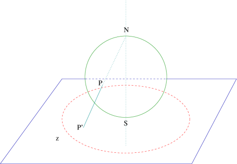
Figure 1: Map from the sphere to the tangent plane at the south pole.

The hermitean metric is obtained from a real Kähler potential

$$g_{z\bar{z}}=K_{,z\bar{z}},\hskip 20.00003ptK(\bar{z},z)=\ln(1+\bar{z}z)$$ (9)

The complex co-ordinates cover the whole sphere minus the north pole $N$. Observe, that this particular projection maps the equator to the unit circle, the southern hemisphere to its interior, and the northern hemisphere to its exterior.

A second map including the north pole is obtained by inversion of the co-ordinates, i.e. the holomorphic co-ordinate transformation

$$\zeta=\frac{1}{z},\hskip 20.00003pt\bar{\zeta}=\frac{1}{\bar{z}}.$$ (10)

The $\zeta$-plane is the plane tangent to the north pole; it defines a complex co-ordinate system covering the sphere minus the south pole, as in figure 2. This is easily observed, as again the equator is projected onto the unit circle, but now the southern hemisphere is mapped to the exterior, and the northern hemisphere is mapped to the interior; in particular the north pole corresponds to the origin $\zeta=0$. Furthermore, the inversion does not change the expression for the line element. This is easy to understand on the basis of symmetry: no matter where the tangent plane is constructed, the spherical symmetry implies that the line element will always be of the form

$$ds^{2}=\frac{d\bar{\zeta}d\zeta}{(1+\bar{\zeta}\zeta)^{2}}.$$ (11)

Note, that inversion changes the Kähler potential to

$$K[\bar{z}(\bar{\zeta}),z(\zeta)]=\ln\left(1+\frac{1}{\bar{\zeta}\zeta}\right)=\ln\left(1+\bar{\zeta}\zeta\right)+F(\zeta)+\bar{F}(\bar{\zeta}),$$ (12)

Nsphere.eps

Figure 2: Map from the sphere to the tangent plane at the north pole.

where $F(\zeta)=-\ln\zeta$ modulo an arbitrary imaginary constant. It follows immediately, that

$$g_{,\zeta\bar{\zeta}}=K_{,\zeta\bar{\zeta}}=\frac{1}{(1+\bar{\zeta}\zeta)^{2}},$$ (13)

as expected.

3 Symmetries of the sphere

The sphere is by definition invariant under rotations around three independent axes. We consider an arbitrary infinitesimal rotation (a rotation close to the identity) over angles $(\varphi,\vartheta,\eta)$. The corresponding change in projection of a rotated point to the tangent plane corresponds to a change in the complex co-ordinates

$$z^{\prime}=z+\delta z,\hskip 20.00003pt\delta z=i\varphi z+\frac{\vartheta}{2}\left(1+z^{2}\right)+\frac{i\eta}{2}\left(1-z^{2}\right).$$ (14)

This is a special holomorphic co-ordinate transformation which leaves the line element of the sphere invariant:

$$\frac{d\bar{z}^{\,\prime}dz^{\prime}}{(1+\bar{z}^{\,\prime}z^{\prime})^{2}}=\frac{d\bar{z}dz}{(1+\bar{z}z)^{2}}.$$ (15)

However, again the Kähler potential is invariant only modulo the real part of a holomorphic function:

$$K^{\prime}(\bar{z}^{\,\prime},z^{\prime})=\ln(1+\bar{z}^{\,\prime}z^{\prime})=K(\bar{z},z)+f(z)+\bar{f}(\bar{z}),$$ (16)

where the holomorphic function is given by

$$f(z)=\frac{1}{2}\left(i\varphi+(\vartheta-i\eta)z\right).$$ (17)

Actually, the purely imaginary $z$-independent part of $f(z)$ is not determined by the transformation of the Kähler potential. We have chosen this particular expression for later convenience. Note, that in general invariance of the Kähler potential modulo the real part of a holomorphic function is sufficient for invariance of the line element:

$$g^{\prime}_{z^{\prime}\bar{z}^{\prime}}(\bar{z}^{\,\prime},z^{\prime})=\frac{\partial{{}^{2}K^{\prime}}}{\partial{z^{\prime}\partial\bar{z}^{\,\prime}}}\,=\frac{1}{\left(1+\bar{z}^{\,\prime}z^{\prime}\right)^{2}}=g_{z\bar{z}}(\bar{z}^{\prime},z^{\prime}).$$ (18)

A vector field $\xi(z)=\delta z$ which, like (14), defines an infinitesimal co-ordinate transformation leaving the line element invariant, is called a Killing vector. The idea carries over directly to higher-dimensional manifolds: on an $N$-dimensional complex manifold a (holomorphic) Killing vector is a (holomorphic) transformation

$$z^{\prime\,i}=z^{i}+\xi^{i}(z),\hskip 20.00003pt\bar{z}^{\prime\,\underline{i}}=\bar{z}^{i}+\bar{\xi}^{\,\underline{i}}(\bar{z}),$$ (19)

such that the line element is invariant:

$$ds^{2}=g_{i\underline{i}}(\bar{z},z)\,d\bar{z}^{\underline{i}}\,dz^{i}=g_{i\underline{i}}(\bar{z}^{\prime},z^{\prime})\,d\bar{z}^{\prime\,\underline{i}}\,dz^{\prime\,i}.$$ (20)

This happens, if the transformation $(\bar{\xi}^{\,\underline{i}}(\bar{z}),\xi^{i}(z))$ satisfies the condition

$$\frac{\partial{\xi_{\underline{i}}}}{\partial{z^{i}}}+\frac{\partial{\bar{\xi}_{i}}}{\partial{\bar{z}^{\underline{i}}}}=0,$$ (21)

where $\xi_{\underline{i}}=g_{i\underline{i}}\,\xi^{i}$ and $\bar{\xi}_{i}=g_{i\underline{i}}\,\bar{\xi}^{\underline{i}}$. We will encounter more examples of such Killing vector fields later on.

4 Cosets

There is another way of looking at the sphere, in terms of groups and cosets. In this section we describe how the sphere can be identified with the coset $SU(2)/U(1)$.

Consider an element $a$ of $SU(2)$. By definition it is a unitary $2\times 2$ matrix with unit determinant: $aa^{\dagger}=1$, $\det a=1$. All elements in the neighborhood of the identity can be parametrized in terms of a real parameter $\alpha$ and a complex parameter $z$ by

$$a(\bar{z},z;\alpha)=\frac{e^{i\alpha\tau_{3}}}{\sqrt{1+\bar{z}z}}\,\left(\begin{array}[]{cc}1&z\\ -\bar{z}&1\end{array}\right).$$ (22)

Note, that the complete $\alpha$-dependence is in the $U(1)$ factor $\exp(i\alpha\tau_{3})$. The class of all elements corresponding to the same value of $(\bar{z},z)$ is therefore a set of elements of $SU(2)$ differing only by a $U(1)$ factor; the set of all such equivalence classes is the coset $SU(2)/U(1)$. A representative of each equivalence class can be chosen by fixing the $U(1)$ gauge to $\alpha=0$:

$$\tilde{a}(\bar{z},z)=a(\bar{z},z;0)=\frac{1}{\sqrt{1+\bar{z}z}}\left(\begin{array}[]{cc}1&z\\ -\bar{z}&1\end{array}\right).$$ (23)

Thus we can associate one element of the coset (an element in the neighborhood of the identity) represented by $\tilde{a}$ with each point in the complex plane. However, there is one element of the coset which is not in the neighborhood of the identity, as it is not associated with any point in the (finite) plane: the element

$$\tilde{a}_{\infty}=\left(\begin{array}[]{cc}0&1\\ -1&0\end{array}\right).$$ (24)

In the present approach this element can be reached by an inversion of the co-ordinates: $\zeta=1/z$, and a change of gauge by multiplying with the $U(1)$ element $\exp(i\theta\tau_{3})$, where $\theta=\arg z=-\arg\zeta$:

$$a(\bar{\zeta}^{-1},\zeta^{-1};\theta)=\frac{1}{\sqrt{1+\bar{\zeta}\zeta}}\left(\begin{array}[]{cc}e^{-i\theta}\sqrt{\bar{\zeta}\zeta}&1\\ -1&e^{i\theta}\sqrt{\bar{\zeta}\zeta}\end{array}\right)=\frac{1}{\sqrt{1+\bar{\zeta}\zeta}}\left(\begin{array}[]{cc}\zeta&1\\ -1&\bar{\zeta}\end{array}\right),$$ (25)

It is then obvious that

$$\tilde{a}_{\infty}=\lim_{\zeta\rightarrow 0}a(\bar{\zeta}^{-1},\zeta^{-1};\theta).$$ (26)

Thus the elements of the coset are actually in one-to-one correspondence with the points on the sphere, rather than with the points in the complex plane.

Not only is there a one-on-one map between coset $SU(2)/U(1)$ and the sphere, this map also respects the symmetries of the sphere, as we now explain. Consider any element $\tilde{a}(\bar{z},z)$ of the coset in the gauge $\alpha=0$. By construction it is also an element of $SU(2)$. We can multiply $\tilde{a}$ from the right with an other element $g$ of $SU(2)$, to get the new element $a_{g}=\tilde{a}g$. In general this will not be an element satisfying the gauge condition $\alpha=0$. It is possible to get back to this gauge by multiplying the element $\alpha_{g}$ from the left by a $g$- and point-dependent $U(1)$ transformation $h_{g}(\tilde{a})$, such that

$$\tilde{a}_{g}=h_{g}\tilde{a}g=\frac{1}{\sqrt{1+\bar{z}_{g}z_{g}}}\left(\begin{array}[]{cc}1&z_{g}\\ -\bar{z}_{g}&1\end{array}\right).$$ (27)

In this way any $SU(2)$ transformation $g$ maps a coset element $\tilde{a}$ labeled by parameters $(\bar{z},z)$ to another element $\tilde{a}_{g}$ labeled by $(\bar{z}_{g},z_{g})$. Explicitly, for an infinitesimal transformation

$$g\simeq\left(\begin{array}[]{cc}1-i\varphi/2&(\vartheta+i\eta)/2\\ -(\vartheta-i\eta)/2&1+i\varphi/2\end{array}\right),$$ (28)

there is a compensating $U(1)$ transformation

$$h_{g}(\bar{z},z)\simeq\left(\begin{array}[]{cc}1+i\alpha(\bar{z},z)&0\\ 0&1-i\alpha(\bar{z},z)\end{array}\right),$$ (29)

with

$$\alpha(\bar{z},z)=\frac{1}{2i}\left(f(z)-\bar{f}(\bar{z})\right),$$ (30)

such that $\tilde{a}_{g}$ is given by the r.h.s. of (27) with

$$z_{g}\simeq z+\delta z,\hskip 20.00003pt\delta z=i\varphi z+\frac{\vartheta}{2}\left(1+z^{2}\right)+\frac{i\eta}{2}\left(1-z^{2}\right).$$ (31)

as in eq.(14); $f(z)$ in eq.(30) is given by the expression (17), which justifies a posteriori our choice of the constant imaginary term in $f(z)$. In conclusion, we see that the symmetries of the sphere (rotations) are realized as non-linear $SU(2)$ transformations on the coset elements $\tilde{a}(\bar{z},z)$. Therefore, the invariant line element on the sphere (8) also defines an $SU(2)$-invariant line element on the coset $SU(2)/U(1)$.

5 Field theory on cosets: the non-linear $\sigma$-model

We have seen how a non-linear realization of $SU(2)$ can be constructed in terms of coset elements. We have also constructed an invariant line element on the coset. It is then straightforward to write down a theory of a massless complex scalar field $z(x)$ in a $n$-dimensional space-time, which is invariant under the non-linear $SU(2)$ transformations (31). It is based on the invariant action

$$S[\bar{z},z]=-\int d^{n}x\,\frac{\partial\bar{z}\cdot\partial z}{(1+\bar{z}z)^{2}}.$$ (32)

As our discussions above show, this action can only be used for fluctuations of the field not too far from the identity $(\bar{z}=z=0)$. For large fluctuations which include the pole of the sphere at $z=\infty$, a second chart from the sphere to the complex plane is needed. Another limitation is, that the model is not renormalizable beyond $n=2$; therefore in $4$-$d$ space-time such a field theory is at best an effective theory for light scalar degrees of freedom in a theory with broken $SU(2)$.

It is known from Goldstone’s theorem, that in fact such massless scalars always arise in a theory with a spontaneously broken rigid symmetry, either as elementary or composite states. For the case of elementary fields it is easy to show. Suppose that we have a triplet of (real) scalar fields $\phi_{i}$, $i=(1,2,3)$, with an action

$$S[\vec{\phi}]=-\int d^{n}x\,\left(\frac{1}{2}\,(\partial\vec{\phi})^{2}+V[\vec{\phi}^{\,2}]\right).$$ (33)

As the potential depends only on the modulus $\vec{\phi}^{\,2}$, the action is invariant under $SO(3)\simeq SU(2)$ transformations rotating the 3-vector $\vec{\phi}$ whilst keeping its length fixed. Suppose the lowest energy state of the theory is such that the field has a non-zero expecation value: $\vec{\phi}^{\,2}=1/f^{2}$. Then the low-energy behaviour of the theory is dominated by the fluctuations of $\vec{\phi}$ respecting the fixed length; these can be parametrized by writing

$$\begin{array}[]{l}\displaystyle{\phi_{1}=\rho\,\sin\vartheta\cos\varphi,\hskip 20.00003pt\phi_{2}=\rho\,\sin\vartheta\sin\varphi,}\\ \\ \displaystyle{\phi_{3}=\rho\,\cos\vartheta.}\end{array}$$ (34)

Taking $\rho=1/f$ fixed, and inserting this parametrization back into the action (33), we obtain

$$S[\vec{\phi}]\rightarrow\frac{1}{f^{2}}\,\int d^{n}x\,\left[(\partial\vartheta)^{2}+\sin^{2}\vartheta\,(\partial\varphi)^{2}+V[1/f^{2}]\right].$$ (35)

A comparison with eq.(8) shows that up to an additive constant $V[1/f^{2}]$, and with the normalization $f=2$, this reduces to the action (32). On the other hand, keeping the radial degree of freedom $\rho$ in the theory, one easily deduces that it has a mass $m_{\rho}^{2}=\partial^{2}V/\partial\rho^{2}$ (evaluated at $\rho=1/f$). This establishes that the range of energies, in which the effective action (32) is valid, is $-Q^{2}\leq m_{\rho}^{2}$. If the symmetry discussed is broken at very high energies, such as in GUT models, this regime can of course be very large ($m_{\rho}\sim 10^{15}$ GeV).

6 Dressing the sphere

In the following we extend this construction to supersymmetric field theories. To this end we have to include additional fields also transforming under some non-linear (spontaneously broken) version of $SU(2)$, or some larger Lie group in more general cases. The key to finding representations of the non-linear transformations is by their identification as special holomorphic co-ordinate transformations. This implies, that if we have representations of the group of general co-ordinate transformations, we directly obtain representations of $SU(2)$ by restricting the co-ordinate transformations to those generated by the Killing vectors (14).

The simplest representations we can construct are those based on standard representations of the group of general co-ordinate transformations: scalars, vectors and tensors. A scalar $S(\bar{z},z)$ takes the same value at the same point, independent of the co-ordinate system; hence under an infinitesimal holomorphic co-ordinate transformation

$$z^{\prime}=z+\xi(z),\hskip 20.00003pt\bar{z}^{\prime}=\bar{z}+\bar{\xi}(\bar{z}),$$ (36)

the scalar transforms to first order in $(\bar{\xi},\xi)$ as

$$S^{\prime}(\bar{z}^{\prime},z^{\prime})=S(\bar{z},z)\hskip 10.00002pt\Rightarrow\hskip 10.00002ptS^{\prime}(\bar{z},z)-S(\bar{z},z)=-\xi(z)\,\partial S(\bar{z},z)-\bar{\xi}(\bar{z})\,\bar{\partial}S(\bar{z},z).$$ (37)

Applying the same rule to the components of a holomorphic one-form $A(\bar{z},z)$ $=A_{z}(\bar{z},z)\,dz$ one finds:

$$A^{\prime}_{z}(\bar{z},z)-A_{z}(\bar{z},z)=-\partial\xi(z)A_{z}(\bar{z},z)-\xi(z)\,\partial A_{z}(\bar{z},z)-\bar{\xi}(\bar{z})\,\bar{\partial}A_{z}(\bar{z},z).$$ (38)

For the components of a vector $V(\bar{z},z)=V^{z}(\bar{z},z)\,\partial$ we find the contragredient transformation:

$$V^{\prime\,z}(\bar{z},z)-V^{z}(\bar{z},z)=\partial\xi(z)V^{z}(\bar{z},z)-\xi(z)\,\partial V^{z}(\bar{z},z)-\bar{\xi}(\bar{z})\,\bar{\partial}V^{z}(\bar{z},z).$$ (39)

This guarantees that the contraction of a vector and a one-form of the same type (e.g., $V^{z}A_{z}$) transforms as a scalar. In addition to holomorphic one-forms and vectors, there are also anti-holomorphic one-forms and vectors ($\bar{A}=\bar{A}_{\bar{z}}\,d\bar{z}$, $\bar{V}=\bar{V}^{\,\bar{z}}\,\bar{\partial}$), and tensors transforming as direct products of forms and vectors. e.g.:

$$\begin{array}[]{lll}T^{\prime}_{z\bar{z}}(\bar{z},z)-T_{z\bar{z}}(\bar{z},z)&=&\displaystyle{-\partial\xi(z)T_{z\bar{z}}(\bar{z},z)-\bar{\partial}\bar{\xi}(\bar{z})T_{z\bar{z}}(\bar{z},z)}\\ &&\\ &&\displaystyle{-\xi(z)\partial T_{z\bar{z}}(\bar{z},z)-\bar{\xi}(\bar{z})\bar{\partial}T_{z\bar{z}}(\bar{z},z)}\\ &&\\ &=&\displaystyle{-\partial\left(\xi(z)T_{z\bar{z}}(\bar{z},z)\right)-\bar{\partial}\left(\bar{\xi}(\bar{z})T_{z\bar{z}}(\bar{z},z)\right).}\end{array}$$ (40)

In particular, the metric transforms as such a mixed tensor, from which one can immediately deduce the Killing condition (21) for invariance of the line element.

Each of the transformations (37)-(40) can be turned into an $SU(2)$ transformation corresponding to the element $g(\varphi,\vartheta,\eta)$ by restricting $(\xi(z),\bar{\xi}(\bar{z}))$ to the Killing vectors (14):

$$\delta_{g}z=\xi_{g}(z)=i\varphi z+\frac{\vartheta}{2}\left(1+z^{2}\right)+\frac{i\eta}{2}\left(1-z^{2}\right).$$

Line bundles
In addition to the vector and tensor representations constructed in this way,we can define representations based on holomorphic line bundles. The construction starts from the transformation rule of the Kähler potential: $\delta_{\xi}K=F_{\xi}+\bar{F}_{\xi}$, where $\xi$ is a Killing vector and $F_{\xi}$ is a corresponding holomorphic function. A holomorphic line bundle $\Omega(\bar{z},z)$ of weight $\lambda$, defined on the sphere, then transforms under a holomorphic co-ordinate transformation (36) as

$$\begin{array}[]{l}\Omega^{\prime}(\bar{z}^{\prime},z^{\prime})\,=\,\displaystyle{e^{\lambda F_{\xi}(z)}\,\Omega(\bar{z},z)}\\ \\ ~{}~{}\Rightarrow\;\displaystyle{\Omega^{\prime}(\bar{z},z)-\Omega(\bar{z},z)\approx-\xi(z)\,\partial\Omega-\bar{\xi}(\bar{z})\,\bar{\partial}\Omega+\lambda F_{\xi}(z)\Omega(\bar{z},z).}\end{array}$$ (41)

In particular, under an $SU(2)$ transformation defined by the above Killing vector:

$$\Omega_{g}(\bar{z}_{g},z_{g})=e^{\lambda f_{g}(z)}\Omega(\bar{z},z)\approx\Omega(\bar{z},z)+\lambda f_{g}(z)\Omega(\bar{z},z).$$ (42)

This defines a representation of $SU(2)$, as the functions $f_{g}(z)$ have the property

$$f_{g_{2}g_{1}}(z_{g_{2}g_{1}})=f_{g_{2}}(z_{g_{1}})+f_{g_{1}}(z).$$ (43)

Similarly, one can define anti-holomorphic line bundles $\bar{\Omega}(\bar{z},z)$ with the transformation law

$$\bar{\Omega}_{g}(\bar{z}_{g},z_{g})=e^{\lambda\bar{f}_{g}(\bar{z})}\,\bar{\Omega}(\bar{z},z)\approx\bar{\Omega}(\bar{z},z)+\lambda\bar{f}(\bar{z})\Omega(\bar{z},z).$$ (44)

The archetype of a multiplicative line bundle on a Kähler manifold is the exponent of the Kähler potential:

$$E_{\lambda}(\bar{z},z)=e^{\lambda K(\bar{z},z)}.$$ (45)

Under an $SU(2)$ transformation $g(\varphi,\vartheta,\eta)$ of the type above, cf. eqs. (28)-(31), $E_{\lambda}$ transforms as

$$\begin{array}[]{lll}(E_{\lambda})_{g}(\bar{z}_{g},z_{g})&=&\displaystyle{e^{\lambda f_{g}(z)+\lambda\bar{f}_{g}(\bar{z})}\,E_{\lambda}(\bar{z},z)}\\ &&\\ &\approx&\displaystyle{E_{\lambda}(\bar{z},z)+\lambda f_{g}(z)E_{\lambda}(\bar{z},z)+\lambda\bar{f}_{g}(\bar{z})E_{\lambda}(\bar{z},z).}\end{array}$$ (46)

The condition (43) is sufficient to guarantee the group property of the transformations for a line bundle $\Omega(\bar{z},z)$ in any point of the manifold. However, it does not guarantee the existence of the line bundle globally; the global existence of line bundles requires $\lambda\in{\bf Z}$. Indeed, under the transformation $z^{\prime}=1/z$, necessary to cover the full coset (sphere)

$$\Omega^{\prime}(\bar{z}^{\prime},z^{\prime})=\frac{1}{z^{\lambda}}\,\Omega(\bar{z},z),$$ (47)

This is single-valued on the unit circle (the equator of the sphere, where the co-ordinate patches overlap) if and only if $\lambda$ is an integer. A similar quantization condition (the cocycle condition) holds on all compact Kähler cosets.

Finally, combining the various realizations of the non-linear symmetry transformations constructed here, the most general representation of spontaneously broken $SU(2)$ is a combination of vector/tensor- and line-bundles, e.g. a one-form valued mixed holomorphic and anti-holomorphic line bundle with component $A_{z}$ transforms as

$$\begin{array}[]{l}A_{z}^{\prime}(\bar{z},z)-A_{z}(\bar{z},z)=\displaystyle{-\,\partial\xi_{g}(z)\,A_{z}(\bar{z},z)-\xi_{g}(z)\partial A_{z}(\bar{z},z)-\bar{\xi}_{g}(\bar{z})\,\bar{\partial}A_{z}(\bar{z},z)}\\ \\ \displaystyle{\hskip 94.00008pt+\,\left(\lambda f_{g}(z)+\mu\bar{f}_{g}(\bar{z})\right)A_{z}(\bar{z},z),}\end{array}$$ (48)

where $\lambda$ and $\mu$ are integers for global consistency.

7 Supersymmetry on the sphere

With the prescriptions of the previous section at hand we can now construct a theory with supersymmetry in the target space defined by the sphere — or some other Kähler manifold. This construction goes as follows. In $D=4$ space-time a chiral multiplet consists of a complex scalar field $z(x)$ and an anti-commuting chiral spinor $\psi_{L}(x)$. If $z(x)$ takes values on the sphere and carries a representation of spontaneously broken $SU(2)$, then these transformations commute with supersymmetry if we assign to the space-time spinor the transformation rule of a vector over the target space (the sphere):

$$\delta_{g}\psi_{L}=\partial\xi_{g}(z)\,\psi_{L}=\left(i\varphi+(\vartheta-i\eta)z\right)\psi_{L}=2f_{g}(z)\psi_{L}.$$ (49)

Three remarks are in order:
- $\psi_{L}(x)$ is a fluctuating field over space-time, but a constant section of a contravariant vector bundle over the sphere: it is independent of $z$, and therefore its derivatives w.r.t. $z$ vanish.
- Under supersymmetry the scalar field transforms into the chiral spinor $\psi_{L}$; the transformation (49) is precisely such, that supersymmetry and $SU(2)$ commute:

$$\delta_{Q}z=\bar{\epsilon}_{R}\psi_{L}\hskip 10.00002pt\Rightarrow\hskip 10.00002pt\left[\delta_{g},\delta_{Q}\right]z=0.$$ (50)

- For the special case of the sphere it happens, that a vector transforms as a line bundle of weight $2$; this is not true for general Kähler manifolds.

The whole construction is equivalent to starting with a chiral superfield

$$\Phi(x,\theta)=z(x)+\bar{\theta}_{R}\psi_{L}(x)+\bar{\theta}_{R}\theta_{L}H(x)+...,$$ (51)

where $\theta_{L}$ is an anticommuting spinor co-ordinate, and $H$ is a complex auxiliary scalar field. Under $SU(2)$ this superfield transforms in the non-linear representation (14):

$$\delta\Phi=\xi_{g}[\Phi]=i\varphi\,\Phi+\frac{\vartheta}{2}\left(1+\Phi^{2}\right)+\frac{i\eta}{2}\left(1-\Phi^{2}\right).$$ (52)

The action of $SU(2)$ on the component fields can then be read off from a comparison of terms with the same $\theta$ dependence on both sides of the equation. The construction of an invariant action for the chiral multiplet is straightforward: first construct the real superfield-valued Kähler potential

$$K(\bar{\Phi},\Phi)=\ln\left(1+\bar{\Phi}\Phi\right);$$ (53)

then take the superspace integral ($D$-term) of this real superfield:

$$S=\int d^{4}x\int d^{2}\theta_{L}\int d^{2}\theta_{R}\,K(\bar{\Phi},\Phi).$$ (54)

Written out in space-time components and eliminating the auxiliary fields one obtains

$$S=-\int d^{4}x\,\left(\frac{\partial\bar{z}\cdot\partial z}{(1+\bar{z}z)^{2}}+\frac{\bar{\psi}_{L}\stackrel{{\scriptstyle\leftrightarrow}}{{D/\hskip 0.86108pt}}\psi_{L}}{(1+\bar{z}z)^{2}}-\frac{(\bar{\psi}_{L}\gamma_{\mu}\psi_{L})^{2}}{(1+\bar{z}z)^{4}}\right).$$ (55)

Here the covariant derivative of the spinor field is defined as the pull-back of the Kähler connection on the sphere:

$$D/\hskip 0.86108pt\psi_{L}=\left(\partial/+\partial/z\,\Gamma_{zz}^{\;\;\;z}\right)\psi_{L}=\left(\partial/-\frac{2\bar{z}\partial/z}{(1+\bar{z}z)^{2}}\right)\psi_{L}.$$ (56)

The first purely bosonic term of this action is precisely that of the non-linear $\sigma$-model on the sphere, cf. eq.(32). The fermionic terms are dictated completely by the invariance of the action (modulo total divergences) under supersymmetry transformations of the type (50).

8 Anomalies

The action (55) is invariant under both supersymmetry and $SU(2)$; now $SU(2)$, in particular its linear subgroup $U(1)$, acts non-trivially on the chiral spinor $\psi_{L}$, cf. eq.(49). It is well-known that such a group action on chiral fermions is anomalous in the quantum theory: although the action is invariant, for a single chiral fermion there is no invariant path-integral measure. The discussion can be simplified by redefining the fermion field:

$$\chi_{L}=e^{-K(\bar{z},z)}\,\psi_{L}=\frac{\psi_{L}}{1+\bar{z}z}.$$ (57)

In terms of this field the action (55) takes the form

$$S=-\int d^{4}x\left(\frac{\partial\bar{z}\cdot\partial z}{(1+\bar{z}z)^{2}}+\bar{\chi}_{L}\stackrel{{\scriptstyle\leftrightarrow}}{{D/\hskip 0.86108pt}}\chi_{L}-\left(\bar{\chi}_{L}\gamma_{\mu}\chi_{L}\right)^{2}\right),$$ (58)

with the covariant derivative

$$D/\hskip 0.86108pt\chi_{L}=\left(\partial/-iV/\hskip 0.86108pt\right)\chi_{L},\hskip 20.00003ptV_{\mu}=-i\,\frac{\bar{z}\stackrel{{\scriptstyle\leftrightarrow}}{{\partial}}_{\mu}z}{1+\bar{z}z}.$$ (59)

By construction this connection renders the derivative covariant under field-dependent $U(1)$ transformations

$$(\chi_{L})_{g}=e^{f_{g}(z)-\bar{f}_{g}(\bar{z})}\,\chi_{L}\approx(1+f_{g}(z)-\bar{f}_{g}(\bar{z}))\chi_{L},$$ (60)

which is the equivalent of the field-dependent $SU(2)$ transformation of $\psi_{L}$, eq.(49).

As the kinetic fermion term in (58) is of the standard form, the usual triangle anomaly calculation applies, and the $U(1)$ current, as well as its parent $SU(2)$ currents, are not conserved. The quantum theory then is inconsistent [20]-[25]. One way to repair this situation is to introduce another chiral multiplet, which we refer to as ‘matter multiplet’,

$$A(x,\theta)=a(x)+\bar{\theta}_{R}\phi_{L}(x)+\bar{\theta}_{R}\theta_{L}N(x)+...$$ (61)

transforming as a holomorphic line bundle of weight $-2$:

$$A_{g}=e^{-2f_{g}(\Phi)}\,A.$$ (62)

Note, that the holomorphicity is important to guarantee the chiral superfield nature of the transformed superfield.

For the chiral superfield $A$ one can construct an invariant action from the superspace expression

$${\cal L}_{matter}=e^{2K(\bar{\Phi},\Phi)}\,\bar{A}A,$$ (63)

integrated over all of superspace [29]. If one redefines the chiral fermion $\phi_{L}$ by

$$\eta_{L}=e^{K(\bar{z},z)}\phi_{L}=(1+\bar{z}z)\phi_{L},$$ (64)

it has the opposite $U(1)$ transformation property compared to the quasi-Goldstone fermion $\chi_{L}$:

$$(\eta_{L})_{g}=(1-f_{g}(z)+\bar{f}_{g}(\bar{z})+\,{\cal O}(a))\,\eta_{L}.$$ (65)

In the $U(1)$-invariant vacuum (i.e., $\langle a\rangle=0$), the kinetic terms of this fermion in the action (63) then become

$$\Delta{\cal L}_{matter}=\bar{\eta}_{L}\stackrel{{\scriptstyle\leftrightarrow}}{{D/\hskip 0.86108pt}}\eta_{L}+...,\hskip 20.00003ptD/\hskip 0.86108pt\eta_{L}=\left(\partial/+iV/\hskip 0.86108pt\right)\eta_{L}.$$ (66)

As the effective $U(1)$ charge of the matter fermion $\eta_{L}$ is opposite to that of the quasi-Goldstone fermion $\chi_{L}$, their triangle anomalies cancel. The mechanism explained here to eliminate anomalies in supersymmetric theories on Kähler manifolds using holomorphic line-bundle representations of symmetry groups works quite generally [26].

9 Gauging of internal symmetries

Let me summarize the results of the previous sections. The supersymmetric model on the coset $SU(2)/U(1)$, defined by the two chiral superfields $(\Phi,A)$ and the Kähler potential

$$K[\bar{\Phi},\Phi;\bar{A},A]=\ln(1+\bar{\Phi}\Phi)+(1+\bar{\Phi}\Phi)^{2}\bar{A}A,$$ (67)

is invariant under the non-linear $SU(2)$ transformations

$$\begin{array}[]{l}\displaystyle{\delta\Phi=\epsilon+i\varphi\,\Phi+\bar{\epsilon}\,\Phi^{2},\hskip 20.00003pt\delta A=-i\varphi A-2\bar{\epsilon}\,\Phi A,}\\ \\ \displaystyle{\epsilon=\frac{1}{2}\left(\vartheta+i\eta\right),\hskip 20.00003pt\bar{\epsilon}=\frac{1}{2}\left(\vartheta-i\eta\right).}\end{array}$$ (68)

As the two chiral fermions in the model carry opposite charges, the internal symmetry is free of anomalies. This allows us to promote the model to a consistent quantum field theory e.g. using path-integral quantization. Of course, the model is not renormalizable, hence it must be regarded as an effective quantum field theory, decribing the physical degrees of freedom in a limited range of energies/distance scales.

A second important benefit from the absence of anomalies and the resulting current conservation is, that the internal symmetry can be gauged consistently. Because of the interplay with supersymmetry, gauging the $SU(2)$ symmetry involves several steps. The first step is to extend all derivatives to covariant derivatives, introducing gauge fields $(W^{+}_{\mu},A_{\mu},W^{-}_{\mu})$ for the transformations parametrized by $(\epsilon,\varphi,\bar{\epsilon})$, respectively. For example, the covariant derivatives on the scalars act as

$$D_{\mu}z=\partial_{\mu}z-g(W^{+}_{\mu}+iA_{\mu}z+W^{-}_{\mu}z^{2}),\hskip 10.00002ptD_{\mu}a=\partial_{\mu}a+g(iA_{\mu}+2W^{-}_{\mu}z)\,a.$$ (69)

In the second step, one adds associated Yukawa couplings of the complex scalars $(z,a)$ to the fermions $(\psi_{L},\phi_{L})$ and the gauginos $(\lambda^{+},\lambda,\lambda^{-})$, the superpartners of the gauge fields. And finally one has to add a potential which results from eliminating the auxiliary fields $(D^{+},D,D^{-})$ associated with the gauge fields by supersymmetry. We will not present the full action here; it can been found in ref.[29]. However, the $D$-term potential is of special interest, and we discuss it in some detail.

I first return to eq.(21) defining the holomorphic Killing vectors $\xi^{i}(z)$. This equation implies, that at least locally for any Killing vector there exists a real function $M(\bar{z},z)$ such that

$$\xi_{\underline{i}}=g_{i\underline{i}}\,\xi^{i}=-i\frac{\partial{M}}{\partial{\bar{z}^{\underline{i}}}},\hskip 20.00003pt\bar{\xi}_{i}=g_{i\underline{i}}\,\bar{\xi}^{\underline{i}}=i\frac{\partial{M}}{\partial{z^{i}}}.$$ (70)

Actually an explicit construction of these Killing potentials exists. Consider the Killing vector $\xi_{g}(z)$ associated with the element $g$ of the group of invariances of the line element. We know that under this transformation the Kähler potential behaves as

$$\delta_{g}K=\xi_{g}^{i}\,\frac{\partial{K}}{\partial{z^{i}}}+\bar{\xi}_{g}^{\underline{i}}\,\frac{\partial{K}}{\partial{\bar{z}^{\underline{i}}}}=f_{g}(z)+\bar{f}_{g}(\bar{z})$$ (71)

Now define $M_{g}(\bar{z},z)$ by

$$-iM_{g}=\xi_{g}^{i}\,\frac{\partial{K}}{\partial{z^{i}}}-f_{g}(z)=-\bar{\xi}_{g}^{\underline{i}}\,\frac{\partial{K}}{\partial{\bar{z}^{\underline{i}}}}+\bar{f}_{g}(\bar{z}).$$ (72)

As is obvious from the expressions on the r.h.s., the quantity $M_{g}$ is real. It is straightforward to show, that $M_{g}$ is the Killing potential for $\xi_{g}^{i}(z)$; indeed, as both $\xi^{i}_{g}(z)$ and $f_{g}(z)$ are holomorphic,

$$-i\frac{\partial{M_{g}}}{\partial{\bar{z}^{\underline{i}}}}=\xi_{g}^{i}\,\frac{\partial{{}^{2}K}}{\partial{\bar{z}^{\underline{i}}\partial z^{i}}}=g_{i\underline{i}}\,\xi_{g}^{i}=\xi_{g\,\underline{i}}.$$ (73)

Applying this construction to the coset model on $SU(2)/U(1)$ we find the explicit expressions

$$-iM_{g}(\bar{\Phi},\Phi;\bar{A},A)=\frac{-i\varphi\,(1-\bar{\Phi}\Phi)+2(\epsilon\bar{\Phi}-\bar{\epsilon}\Phi)}{1+\bar{\Phi}\Phi}\left(\frac{1}{2}\,+\left(1+\bar{\Phi}\Phi\right)^{2}\bar{A}A\right).$$ (74)

Note, that if one computes the gradient of these potentials: $\partial M_{g}/\partial\bar{\Phi}$, $\partial M_{g}/\partial\bar{A}$, one does not recover directly the Killing vectors represented by eqs.(68): there is still a metric factor

$$G_{I\underline{I}}=\left(\begin{array}[]{cc}\frac{\partial{{}^{2}K}}{\partial{\bar{\Phi}\partial\Phi}}&\frac{\partial{{}^{2}K}}{\partial{\bar{\Phi}\partial A}}\\ \\ \frac{\partial{{}^{2}K}}{\partial{\bar{A}\partial\Phi}}&\frac{\partial{{}^{2}K}}{\partial{\bar{A}\partial A}}\end{array}\right),$$ (75)

to take into account.

Returning to the subject of the $D$-term potential, it can be shown quite generally that elimination of the auxilary $D$-fields leads to a scalar potential

$$V_{D}(\bar{z},z;\bar{a},a)=\frac{g^{2}}{2}\,D_{a}^{2}=\frac{g^{2}}{2}\,M_{a}^{2}(\bar{z},z;\bar{a},a),$$ (76)

where the sum is over all independent components of the Lie-algebra of isometries, labeled by $a$. For the case of the coset $SU(2)/U(1)$ this becomes explicitly

$$V_{D}=\frac{g^{2}}{2}\frac{\partial{M_{g}}}{\partial{\epsilon}}\frac{\partial{M_{g}}}{\partial{\bar{\epsilon}}}+\frac{g^{2}}{2}\left(\frac{\partial{M_{g}}}{\partial{\varphi}}\right)^{2}=\frac{g^{2}}{2}\left(\frac{1}{2}\,+(1+\bar{z}z)^{2}\bar{a}a\right)^{2}.$$ (77)

From the explicit form of the potential we learn two important physical facts:
- The potential is positive definite, with a minimum at $V_{D}=g^{2}/8$; this implies that supersymmetry is spontaneously broken.
- The minimum is reached for $z=a=0$; hence the linear $U(1)$ symmetry is not spontaneously broken, and the $U(1)$ gauge field $A_{\mu}$ remains massless.
We observe at the same time, that the charged vector bosons $W^{\pm}_{\mu}$ become massive. This is most easily seen by going to the unitary gauge, in which $\bar{z}=z=0$; then the covariant derivative of $z$, eq.(69), reduces to $-gW_{\mu}^{+}$, and the former kinetic terms for the Goldstone bosons become

$${\cal L}_{kin}(\bar{z},z)=-g^{2}W^{+}\cdot W^{-}.$$ (78)

I refer to [29] for details.

10 Extensions to larger coset manifolds

The action of a supersymmetric field theory in 4-$D$ space-time constructed from chiral supermultiplets $(z^{i},\psi_{L}^{i})$, $i=1,...,r$, is defined by two functions of the superfields: the real Kähler potential $K(\bar{\Phi},\Phi)$, and the holomorphic superpotential $W(\Phi)$. In components the action reads

$$\begin{array}[]{lll}{\cal L}&=&\displaystyle{-g_{i\underline{i}}\left(\partial\bar{z}^{\,\underline{i}}\cdot\partial z^{i}+\frac{1}{2}\,\bar{\psi}_{L}^{\underline{i}}\stackrel{{\scriptstyle\leftrightarrow}}{{D/\hskip 0.86108pt}}\psi_{L}^{i}\right)-g^{\underline{i}i}\bar{W}_{;\underline{i}}W_{;i}}\\ &&\\ &&\displaystyle{+\,W_{;ij}\,\bar{\psi}^{i}_{R}\psi_{L}^{j}+\bar{W}_{;\underline{i}\underline{j}}\,\bar{\psi}_{L}^{\underline{i}}\psi_{R}^{\underline{j}}+\frac{1}{8}\,R_{i\underline{i}j\underline{j}}\,\bar{\psi}_{L}^{\underline{i}}\gamma^{\mu}\psi_{L}^{i}\,\bar{\psi}_{R}^{\underline{j}}\gamma_{\mu}\psi_{R}^{\underline{i}}.}\end{array}$$ (79)

Here $g_{i\underline{i}}=K_{,i\underline{i}}$ is the Kähler metric, $D/\hskip 0.86108pt$ the covariant derivative on the Kähler manifold and $R_{i\underline{i}j\underline{j}}$ the corresponding curvature tensor. There are many cosets of Kähler type of interest for particle physics phenomenology; these include the Grasmannian models on $SU(N+M)/S[U(N)\times U(M)]$, such as the GUT-like model $SU(5)/SU(3)\times SU(2)\times U(1)$.

To reproduce the particle content of the standard model, as summarized in table 1, the internal symmetries of such a model must be promoted to local symmetries, by coupling to appropriate non-abelian vector multiplets; this is possible only if the symmetries are non-anomalous. Like in the model on $SU(2)/U(1)$, this is generically not the case. The model on $SU(5)/SU(3)\times SU(2)\times U(1)$ provides a typical example. The Goldstone superfields in this model are $\Phi^{\alpha r}$, where $\alpha=(1,2)$ is an $SU(2)$ index and $r=(1,2,3)$ an $SU(3)$ index; thus they transform as a doublet-triplet of $SU(2)\times SU(3)$. In particular, the fermion components carry the quantum numbers of left-handed quark doublets. By itself this set of chiral fermions forms an anomalous representation of $SU(3)\times SU(2)\times U(1)$.

As in the $SU(2)/U(1)$ model, the anomalies can be canceled by incorporating additional supermultiplets. Actually the standard model suggests how to do this: introduce chiral superfields with the $SU(3)\times SU(2)$ quantum numbers of lepton doublets, plus superfields containing anti-quark and anti-lepton $SU(2)$ singlets. Indeed, this suffices to guarantee the absence of anomalies of the full parent $SU(5)$ symmetry, provided the chiral fermions have the correct $U(1)$ hypercharges. Observe, that to obtain full agreement with the spontaneously broken standard model including at least one family of quarks and leptons, one needs to introduce a Higgs and an anti-Higgs doublet with opposite hypercharges as well; with this hypercharge assignment the higgsinos do not cause new anomalies. Details of this model can be found in [27].

To realize the correct hypercharge assignments of the additional superfields is not trivial. For example, the left-handed anti-electron is an $SU(2)$ and $SU(3)$ singlet, suggesting that it should be part of a superfield $\Phi$ which is a singlet under $SU(3)\times SU(2)\times U(1)$; however, its true $U(1)$ hypercharge is $+1$. Such a hypercharge assignment can be realized by promoting $\Phi$ to a line-bundle representation of $SU(5)$, generalizing the construction I presented for $SU(2)/U(1)$. The required line-bundle representation actually exists, not only for the left-handed anti-electron, but for all chiral superfields containing standard-model fermions and Higgs doublets [27]. Thus line bundle representations play a crucial role in eliminating anomalies, not only in the simple $SU(2)/U(1)$ model, but also in the larger models which are more interesting from the phenomenological point of view.

Once the anomalies have been canceled, the $SU(5)$ symmetry can be gauged in a way that respects the supersymmetry of the action. In broad outline the following happens:
- First, a set of 24 vector multiplets $(A_{\mu}^{a},\lambda^{a},D^{a})$ is introduced as required by local $SU(5)$ symmetry.
- Gauging the action whilst preserving supersymmetry gives rise to covariant derivatives, accompanied by Yukawa couplings and a $D$-term potential, defined in terms of the Killing potentials for the $SU(5)$ isometries.
- The vector bosons corresponding to broken directions in $SU(5)$ become massive, but the vector bosons corresponding to the linear $SU(3)\times SU(2)\times U(1)$ subgroup remain massless, at least as long as there are no vacuum expectation values for the Higgs doublets.
- The Goldstone bosons $z^{i}$ disappear from the spectrum of physical states; this is manifest in the unitary gauge $z^{i}=0$, which can always be realized if the parameters of the non-linear $SU(5)$ transformations become space-time dependent. As a result, in these supersymmetric models only the quarks and leptons which are part of the additional matter superfields have scalar partners; the quark doublet-triplet has no physical superpartners left. This shows, that the model exhibits strong spontaneous supersymmetry breaking.
- Like the vector bosons, the gauginos split into linear representations of the stability group $SU(3)\times SU(2)\times U(1)$:

$${\bf 24}\hskip 10.00002pt\rightarrow\hskip 10.00002pt({\bf 8},{\bf 1})+({\bf 1},{\bf 3})+({\bf 1},{\bf 1})+({\bf 3},{\bf 2})_{R}+({\bf 3},{\bf 2})_{L}.$$ (80)

The fate of these fermions is quite interesting; first, there are three sets of Majorana gauginos with the same quantum numbers as the massless vector bosons, as expected. Then there is a righthanded doublet-triplet which (in the unitary gauge) combines with the quasi-Goldstone fermions $\psi_{L}$ to form a doublet of massive quarks, with masses of the order of the scale at which $SU(5)$ is broken. And finally, there remains a massless doublet-triplet representing the physical quark doublets in the gauged $\sigma$-model, without physical scalar superpartners.
- The $D$-term potential again takes the form

$$V_{D}=\frac{g^{2}}{2}\,M_{a}^{2},$$ (81)

where $g$ is the $SU(5)$ coupling constant, and the $M_{a}$ are the Killing potentials of the $SU(5)$ transformations. In this expression one may take $\bar{z}^{\underline{i}}=z^{i}=0$ (unitary gauge), i.e. the potential depends only on the physical scalars. It is positive definite, confirming that supersymmetry is broken spontaneously.

The scenario sketched here for the particular model based on the grassmannian coset $SU(5)/SU(3)\times SU(2)\times U(1)$ is representative for a class of models incorporating standard-model like low-energy sectors, e.g.  the models on $SO(10)/U(5)$ and $E_{6}/SO(10)\times U(1)$ [28]; of course the details differ. The coupling of these models to supergravity has been discussed in [27].

11 Conclusions

In these notes I have explained the basic elements of Kähler geometry and its application to the construction of 4-D supersymmetric field theories. In particular I have shown that there exist consistent supersymmetric models with the fermion content and gauge interactions of the standard model, but different from the minimal supersymmetric standard model (MSSM).

In these supersymmetric coset models all or some of the quarks and leptons are quasi-Goldstone fermions, or an equivalent set of unpaired chiral gauginos, lacking physical scalar partners. This strong form of spontaneous supersymmetry breaking clearly distinguishes the physical content of these models from the MSSM or standard supersymmetric GUTs. Of course, this difference affects scenarios of gauge unification and the role of supersymmetry in the solution of the hierarchy problem, although to what extent is presently not clear.

In addition, questions arise as to the possibility of breaking the stability group $H$, which is to be chosen as the standard-model group or a GUT group. In some models we have found that the scalar potential drives the scalar fields to a singular point of the kinetic terms [28, 29]. This may point to a strong coupling regime, possibly with symmetry restauration. Clearly, not all of the physics described by these models is as yet understood.

With the principles of constructing a class of consistent models at hand, the next step is to address physical applications. This part of the work is only about to begin.

References

-
[1]
H.P. Nilles, Phys. Rep. 110 (1984), 1;
id., in: The building blocks of creation, Proc. Adv. Study Inst. El. Part. Phys. (Boulder CO, 1993), 291 - [2] L. Randall and R. Sundrum, Phys. Rev. Lett. 83 (1999), 4690
- [3] J. Bagger and E. Witten, Phys. Lett. B118 (1982), 103
- [4] C.-L. Ong, Phys. Rev. D27 (1983), 911; id., 3044
- [5] M.P. Mattis, Phys. Rev. D28 (1983), 2649
- [6] A.J. Buras and W. Sl/ominski, Nucl. Phys. B223 (1983), 157
- [7] W. Buchmüller, R.D. Peccei and T. Yanagida, Nucl. Phys. B244 (1984), 186
- [8] T. Kugo and T. Yanagida, Phys. Lett. B134 (1984), 313
- [9] Y. Achiman, S. Aoyama and J.W. van Holten, Phys. Lett. B141 (1984), 64; id. B150 (1985), 153; Nucl. Phys. B258 (1985), 179
- [10] J.W. van Holten, Z. Phys. C27 (1985), 57;
- [11] W. Buchmüller and O. Napoly, Phys. Lett. B163 (1985), 161
- [12] T.E. Clark and S.T. Love, Nucl. Phys. B254 (1985), 569
- [13] U. Ellwanger, Nucl. Phys. B281 (1987), 489; Fortschr. Phys. 36 (1988), 881
- [14] J.A. Bagger, Nucl. Phys. B211 (1983), 302
- [15] J.W. van Holten, Nucl. Phys. B260 (1985), 125
- [16] W. Buchmüller and U. Ellwanger, Phys. Lett. B166 (1986), 325
- [17] M. Bando, T. Kugo and K. Yamawaki, Phys. Rep. 164 (1988), 217
- [18] K.J. Barnes, Phys. Lett. B468 (1999), 81
- [19] U. Ellwanger, Nucl. Phys. B356 (1991), 46
- [20] G. Moore and P. Nelson, Phys. Rev. Lett. 53 (1984), 1519
- [21] P. di Vecchia, S. Ferrara and L. Girardello, Phys. Lett. B151 (1985), 199
- [22] D. Nemeschansky and R. Rohm, Nucl. Phys. B249 (1985), 157
- [23] E. Cohen and C. Gómez, Nucl. Phys. B254 (1985), 235
- [24] S. Aoyama and J.W. van Holten, Nucl. Phys. B258 (1985), 18
- [25] W. Buchmüller and W. Lerche, Ann. Phys. 175 (1987), 159
- [26] S. Groot Nibbelink and J.W. van Holten, Phys. Lett. B442 (1998), 185
- [27] S. Groot Nibbelink and J.W. van Holten, Nucl. Phys. B588 (2000), 57
- [28] S. Groot Nibbelink, T.S. Nyawelo and J.W. van Holten, Nucl. Phys. B 594 (2001), 441
- [29] S. Groot Nibbelink, T.S. Nyawelo, F. Riccioni and J.W. van Holten, Nucl. Phys. B663 (2003), 60