Reconstruction of field theory from excitation spectra of defects

Abstract

We show how to reconstruct a field theory from the spectrum of bound states on a topological defect. We apply our recipe to the case of kinks in 1+1 dimensions with one or two bound states. Our recipe successfully yields the sine-Gordon and $\lambda\phi^{4}$ field theories when suitable bound state spectra are assumed. The recipe can also be used to globally reconstruct the inflaton potential of inflationary cosmology if the inflaton produces a topological defect. We discuss how defects can provide “smoking gun” evidence for a class of inflationary models.

I Introduction

Often one is interested in diagonalizing a known operator. This is an eigenvalue problem. The reverse problem, where the eigenvalues are known but the operator is not, is also of interest. This is the “inverse scattering problem” GelLev55 ; Mar55 (also see e.g. Solitonbook ). Indeed it is the basis of the famous question: “Can one hear the shape of a drum?” Kac66 ; GorWebWol92 . In other words, can the frequencies (eigenvalues) of the sound emitted from the drum be used to determine the shape (operator) of the drum? In the quantum mechanics context, the equivalent problem is of reconstructing the Schrodinger potential, $U(x)$, from the energy spectrum. Such inverse scattering problems are of interest in a wide variety of applications.

We will be interested in a class of problems where $U$ itself originates from some field interactions. Our aim is not just to reconstruct the Schrodinger potential, $U$, but the underlying field theory interactions that led to that particular Schrodinger potential. The eigenvalue data that we will use to reconstruct the field theory is the excitation spectra of any topological defects that might be present in the system. The method is widely applicable since topological defects are present in a large class of systems. They are routinely observed in condensed matter systems, and are inevitable in high energy particle physics models. Topological defects relevant for high energy particle physics are also relevant for the very early universe. Hence the excitation spectra of these topological defects can be a window to the early universe, and in particular, to inflationary cosmology.

A way to understand the usefulness of topological defects in a reconstruction effort is that the core of a topological defect contains a different phase of the theory and so the core holds non-perturbative information about the field theory. Therefore the excitation spectrum of the defect leads to a global reconstruction of the field theory. This is in contrast to a local reconstruction that is possible by perturbative methods such as particle scattering.

In what follows, we assume that we are given a topological defect. In fact, for actual calculations, we will exclusively work with kinks in 1+1 dimensions since this example illustrates the central ideas and also because there are extensive techniques in 1+1 dimensions that are not available in higher dimensions. (Although spherically symmetric systems in higher dimensions can be reduced to the 1+1 dimensional case.)

In the next section we will outline the recipe for the reconstruction and then in Sec. III explicitly work through two specific examples with kinks in 1+1 dimensions. Our scheme yields the sine-Gordon field theory when there is only one bound state (the translation mode) on the kink. When the kink has two bound states, we give implicit expressions for the field theory. For a specific choice of the eigenvalues of the two bound states, we obtain the $\lambda\phi^{4}$ field theory. In Sec. IV we discuss the reconstruction problem in the inflationary context. Then we qualitatively discuss the bound state spectrum on kinks made from the inflaton field. In particular, we look for signatures of the flatness of the inflaton potential in the spectrum. Readers only interested in inflation can proceed directly to Sec. IV since the discussion there is largely independent of Sec. II and III.

II General reconstruction scheme

We assume that we know the spectrum of energy eigenvalues, $\{\omega_{i}^{2}\}$, for the bound states on a topological defect. For the time being, we will only focus on the bound states. The price we pay is that there is then a huge degeneracy in the reconstruction. By using scattering information and further physical input it may be possible to eliminate the degeneracy but we shall not be discussing this issue here.

The general reconstruction scheme is as follows.

• Prior to an analysis, a theoretical framework is needed and the appropriate field content should be known. In this discussion we will only consider a single scalar field $\phi$ in one dimension, with standard form of the Lagrangian:

  $$L=\frac{1}{2}(\partial_{\mu}\phi)^{2}-V(\phi)$$ (1)

• The Schrodinger equation that determines the excitation spectrum is:

  $$\left[-\frac{d^{2}}{dx^{2}}+U(x)\right]\psi_{n}=\omega_{n}^{2}\psi_{n}$$ (2)

  where

  $$U(x)=V^{\prime\prime}(\phi_{0}(x))$$ (3)

  and $\phi_{0}(x)$ is the (unknown) profile function of the defect – the classical defect solution. We would like to determine the potential $U(x)$. Inverse scattering methods have been developed precisely to solve this problem. The answer, however, is not unique, especially if only bound state spectra are taken into account. However, additional theoretical input can possibly reduce degeneracies. For example, if some interactions are known by perturbative methods, the information might be useful to break some of the degeneracy.

• Once we have $U(x)$, we find the “translation mode” by solving the zero eigenvalue Schrodinger problem:

  $$\left[-\frac{d^{2}}{dx^{2}}+U(x)\right]\psi_{t}=0$$ (4)

• The translation mode is simply related to the defect profile functions by differentiation:

  $$\psi_{t}(x)=\frac{d\phi_{0}}{dx}$$ (5)

  Hence, we can integrate the translation mode to obtain $\phi_{0}(x)$.

• Next we invert $\phi_{0}(x)$ to obtain $x(\phi_{0})$.

• The equation of motion for the defect is:

  $$-\frac{d^{2}\phi_{0}}{dx^{2}}+V^{\prime}(\phi_{0})=0$$ (6)

  where prime refers to differentiation with respect to the argument. Combining with Eq. (5) we see that:

  $$V^{\prime}(\phi_{0}(x))=\frac{d\psi_{t}}{dx}\bigg{|}_{x(\phi_{0})}$$ (7)

• Finally, an integration yields the desired symmetry breaking potential:

  $$V(\phi_{0})=\int d\phi_{0}V^{\prime}(\phi_{0})$$ (8)

In the 1+1 dimensional case described above, there is actually a slight shortcut that is available to us. In this case, the Bogomolnyi equation holds:

$$\frac{d\phi_{0}}{dx}=\pm\sqrt{2V(\phi_{0})}$$ (9)

and so:

$$V(\phi_{0})=\frac{1}{2}\psi_{t}^{2}\bigg{|}_{x(\phi_{0})}$$ (10)

There are two parts to this recipe. The first is the derivation of $U(x)$ from the eigenvalue spectrum and the second is the derivation of $V(\phi)$ from $U(x)$. The part of the recipe starting with $U(x)$ and constructing $V(\phi)$ as in Eq. (10) has also been used in earlier work LimSanRod02 .

The hardest step in this scheme is step (ii), the reconstruction of $U(x)$ from $\{\omega_{n}^{2}\}$. In 1+1 dimensions (or for S-wave states in 3+1 dimensions), a simple general scheme to reproduce the bound state spectrum is given in Ref. KwoRos86 ; Schetal80 ; Kwoetal80 . The scheme employs the idea of supersymmetric quantum mechanics where the Hamiltonian operator can be factored, and yields a reflectionless potential with the desired bound state spectrum. We now summarize the scheme; a sketch of how the scheme is derived is given in Appendix A. While it may seem that the reconstruction in terms of supersymmetric potentials is overly restrictive, we show in Appendix B that kinks in one spatial dimension always lead to a supersymmetric form of the potential $U(x)$. We also show that this is can be true even when we have multi-component fields in more than one dimension. Thus the reconstruction scheme of KwoRos86 is perfectly suited to our context.

Suppose the bound state eigenvalues are labeled in descending order: $\omega_{i}^{2}>\omega_{i+1}^{2}$ and $i=1,...,N-1$ and the zero energy level is chosen so that the ground state eigenvalue, $\omega_{N}$, is zero. Then a potential containing $n$ of the highest bound states is:

$$U_{n}(x)=f_{n}^{2}+f_{n}^{\prime}+\omega_{n}^{2}$$ (11)

where the function $f_{n}(x)$ satisfies:

$$f_{n}^{\prime}-f_{n}^{2}+U_{n-1}=\omega_{n}^{2}$$ (12)

in terms of $U_{n-1}$, the potential containing $n-1$ of the highest bound states. If we write $f_{n}(x)\equiv-w_{n}^{\prime}/w_{n}$, the equation for $w_{n}$ is:

$$-w_{n}^{\prime\prime}+U_{n-1}w_{n}=\omega_{n}^{2}w_{n}$$ (13)

This equation will have two linearly independent solutions. If we further require that $U_{n}$ be even under parity: $U_{n}(-x)=+U_{n}(x)$, then we need $f_{n}(-x)=-f_{n}(+x)$, and $w_{n}(-x)=w_{n}(+x)$. This condition eliminates one of the linearly independent solutions.

The solution to the $n^{th}$ Schrodinger equation:

$$\left[-\frac{d^{2}}{dx^{2}}+U_{n}(x)\right]\psi_{n}=\omega_{n}^{2}\psi_{n}$$ (14)

is simply:

$$\psi_{n}=\frac{\alpha_{n}}{w_{n}}$$ (15)

where $\alpha_{n}$ is a normalization constant to be determined by other considerations. In particular, since $\omega_{N}$ is the smallest eigenvalue, the corresponding eigenfunction must be the translation mode of the defect that does not affect the energy. Therefore $\omega_{N}=0$ and the translation mode is known once we know $w_{N}$:

$$\psi_{t}=\frac{\alpha}{w_{N}}$$ (16)

where we have dropped the subscript on $\alpha_{N}$. The profile function is:

$$\phi_{0}(x)=\alpha\int\frac{dx}{w_{N}}$$ (17)

and Eq. (10) gives:

$$V(\phi_{0})=\frac{\alpha^{2}}{2w_{N}^{2}}\biggr{|}_{x(\phi_{0})}$$ (18)

The construction of $U_{n}$ is iterative and one must start with the highest bound state with eigenvalue $\omega_{1}^{2}$. To find $w_{1}$ we set $U_{0}=\omega_{0}^{2}$ to be a constant which will be determined by other considerations. Now we illustrate this scheme in a few cases.

III Examples

III.1 One bound state

If the defect has only one bound state, it must be the translation mode. Since translations do not cost energy, the eigenvalue, $\omega_{1}$, vanishes. So we need to solve Eq. (13) with $\omega_{1}=0$:

$$-w_{1}^{\prime\prime}+U_{0}w_{1}=0$$ (19)

with $U_{0}=\omega_{0}^{2}$. After some manipulations:

$$f_{1}=-\omega_{0}\tanh(\omega_{0}x)$$ (20)

and

$$U_{1}(x)=f_{1}^{\prime}+f_{1}^{2}=\omega_{0}^{2}[1-2{\rm sech}^{2}(\omega_{0}x)]$$ (21)

Now we can determine $\omega_{0}$ by the requirement that at spatial infinity, the excitations are the particles in the trivial vacuum. If we denote the masses of these particles by $m$, this means that

$$U(\infty)=m^{2}$$ (22)

Hence: $\omega_{0}=m$ and

$$U(x)=m^{2}[1-2{\rm sech}^{2}(mx)]$$ (23)

The translation mode, $\psi_{t}$, satisfies

$$-\psi_{t}^{\prime\prime}+U(x)\psi_{t}=0$$ (24)

and, in fact, the solution is

$$\psi_{t}=\frac{\alpha}{w_{1}}=\alpha~{}{\rm sech}(mx)$$ (25)

where $\alpha$ is a constant. Note that, in the present context, there is no requirement that $\psi_{t}$ be normalized as a wavefunction.

Therefore the profile function is

$$\phi_{0}(x)=\alpha\int dx~{}{\rm sech}(mx)=\frac{2\alpha}{m}\tan^{-1}\biggl{[}{\rm tanh}\biggl{(}\frac{mx}{2}\biggr{)}\biggr{]}$$ (26)

In other words,

$${\rm tanh}\biggl{(}\frac{mx}{2}\biggr{)}=\tan\biggl{(}\frac{m\phi_{0}}{2\alpha}\biggr{)}$$ (27)

Since here the Bogomolnyi equations can be used, Eq. (10) with some algebra gives:

$$V(\phi_{0})=\frac{\alpha^{2}}{4}\biggl{[}\cos\biggl{(}\frac{2m\phi_{0}}{\alpha}\biggr{)}+1\biggr{]}$$ (28)

This is the sine-Gordon potential.

The potential still contains the unknown parameter $\alpha$. To fix this parameter we could use some other property of the defect, for example, its total energy.

This completes the global reconstruction of the potential in the single bound state case.

III.2 Two bound states

Now there are two eigenvalues $\omega_{1}^{2}$ and $\omega_{2}^{2}$. The translation mode is always the lowest eigenvalue and hence $\omega_{2}^{2}=0$. So we first need to find a potential, $U_{1}(x)$ that contains the $\omega_{1}^{2}$ mode.

Following the recipe given in the previous section, we have

$$U_{1}=f_{1}^{2}+f_{1}^{\prime}+\omega_{1}^{2}$$ (29)

and we need to solve

$$-w_{1}^{\prime\prime}+\omega_{0}^{2}w_{1}=\omega_{1}^{2}w_{1}$$ (30)

where, as before $U_{0}=\omega_{0}^{2}$. This is exactly the single bound state problem that we solved in the previous subsection if we replace $\omega_{0}^{2}$ with $\nu^{2}\equiv\omega_{0}^{2}-\omega_{1}^{2}$. Therefore,

$$f_{1}=-\nu\tanh(\nu x)$$ (31)

and

$$U_{1}=\nu^{2}[1-2{\rm sech}^{2}(\nu x)]+\omega_{1}^{2}$$ (32)

Now we use the second eigenvalue. The potential $U_{2}$ is given by

$$U_{2}=f_{2}^{2}+f_{2}^{\prime}+\omega_{2}^{2}=f_{2}^{2}+f_{2}^{\prime}$$ (33)

where we have used $\omega_{2}^{2}=0$ since this mode must be the translation mode. So we need to solve:

$$-w_{2}^{\prime\prime}+\{\nu^{2}[1-2{\rm sech}^{2}(\nu x)]+\omega_{1}^{2}\}w_{2}=0$$ (34)

We can rescale $z=\nu x$ and bring the equation to the form:

$$\frac{d^{2}w_{2}}{dz^{2}}+\{\lambda+2{\rm sech}^{2}(z)\}w_{2}=0$$ (35)

where:

$$\lambda\equiv-\left[1+\frac{\omega_{1}^{2}}{\nu^{2}}\right]$$ (36)

Eq. (35) has been solved in Ref. MorFes53 (see Section 6.3, page 768) and the solution is given in terms of hypergeometric functions:

$$w_{2} = \{\xi(1-\xi)\}^{K/2}\biggl{[}\vphantom{F}_{2}F_{1}(K+2,K-1;K+1;\xi)$$ (37)

$$+ \vphantom{F}{}_{2}F_{1}(K+2,K-1;K+1;1-\xi)\biggr{]}$$

where,

$$\xi\equiv\frac{1+\tanh(z)}{2}$$ (38)

and

$$K^{2}\equiv-\lambda$$ (39)

Note that we have fixed the ratio of the two linearly independent solutions in Eq. (37) by imposing the requirement that $w_{2}$ have even parity under $z\rightarrow-z$, which is the same as requiring $w_{2}(\xi)=w_{2}(1-\xi)$. (The overall normalization of $w_{2}$ is unimportant.) Now Eq. (18) immediately gives the field theoretic potential though the expression is still implicit since the inverse function, $x(\phi_{0})$, needs to be determined after doing the integral in Eq. (17).

Let us now look at the special case when $\omega_{1}^{2}/\nu^{2}=3$ ($K=2$). Then the solution for $w_{2}$ is given by elementary functions:

$$w_{2}(x)=\cosh^{2}(\nu x)$$ (40)

With this

$$\phi_{0}(x)=\alpha\nu\int\frac{dx}{w_{2}}=\alpha\tanh(\nu x)$$ (41)

where $\alpha$ is a constant of normalization. (For convenience we have explicitly included a factor of $\nu$ in the normalization.) Therefore:

$$V(\phi_{0})=\frac{\alpha^{2}}{2}{\rm sech}^{4}(z)=\frac{\alpha^{2}}{2}\left(1-\frac{\phi_{0}^{2}}{\alpha^{2}}\right)^{2}$$ (42)

Hence we have recovered the $\lambda\phi^{4}$ model in this special case.

It appears remarkable that the simplest examples of one and two bound states have led to two well-known field theories, namely the sine-Gordon and $\lambda\phi^{4}$ theories. A partial explanation is to be found in section B, where we show that whenever $U(x)$ arises from a field theoretic kink, it must necessarily be of the supersymmetric form (Eq. (11)). So the recipe to reconstruct $U(x)$ is ideally suited to the present problem.

III.3 Three or more bound states; higher dimensions

The reconstruction can be continued to the case of three of more bound states. However, the general reconstruction becomes difficult to do analytically and numerical methods are desirable. Such methods have not yet been developed.

The inverse scattering technique that we have used only works in one spatial dimension. Problems in more than one spatial dimension require other inverse scattering techniques. However, if the problem is spherically symmetric, the problem effectively reduces to one spatial dimension and the reconstruction outlined above can be applied. (In Ref. KwoRos86 the authors applied the inverse scattering technique to S-wave bound states of quarks.)

IV Application to cosmological inflation

IV.1 Inflation and defects

If there was an extended but limited period of superluminal expansion in the early universe, light scalar fields would get excited by the spacetime expansion and create adiabatic perturbations on superhorizon scales. The prediction of adiabatic perturbations matches observations of anisotropies in the Cosmic Microwave Background Radiation (CMBR) and is the reason for the current confidence in the cosmic “inflationary” scenario. The mechanism driving cosmic inflation is a scalar field called the “inflaton”. The dynamics of both the spacetime and the scalar field is dominated by the inflaton potential energy for the entire duration of cosmic inflation. Under certain assumptions, this requires the scalar field to lie on top of a very flat potential. With time the scalar field slowly rolls along the flat potential, eventually reaching the steeper parts of the potential where its kinetic energy becomes significant. Then inflation stops and the subsequent evolution of the scalar field leads to “reheating” i.e. conversion of scalar field kinetic energy into ordinary matter in a thermal state.

One hopes that the scalar fields necessary for cosmic inflation will automatically arise in high energy particle physics models, such as Grand Unified Theories (GUTs) or string theory. On very general grounds, it is known that such theories contain magnetic monopoles and sometimes other topological defects. If inflation and the defect are due to separate fields, the study of the defect core cannot yield information about inflation. For the global reconstruction scheme under discussion to work, the inflaton itself should play a role in the structure of the topological defect.

One of the cosmological problems that inflation was designed to solve was the magnetic monopole overabundance problem that arose out of the marriage of GUTs and cosmology. If there is a period of inflation during or after the GUT phase transition, the magnetic monopole density would get diluted to insignificant amounts, leaving perhaps only a few in the entire visible universe. However, subsequent work on inflation has shown that topological defects can still be produced in significant numbers toward the late stages KofLinSta96 ; Tkaetal98 ; KasKaw98 ; Feletal00 ; RajCop00 . If bound states on one of these defects can be studied, it would help in the global reconstruction of the inflaton potential. The other possibility of using the reconstruction scheme is if future particle physics experiments are able to produce magnetic monopole and antimonopole pairs (or closed walls or strings) in the laboratory. The excitations of these monopoles could then be studied. There is also the possibility that duality holds in particle physics and the known particles (e.g. the electron) may be dualized magnetic monopoles Vac96 . The internal excitations of the electron, would then be excitations of a magnetic monopole. Perhaps these excitations can tell us something about inflation.

Earlier work on reconstructing the inflaton potential (see e.g. Lidetal97 ) worked under the assumption that the CMBR anisotropies are generated by quantum fluctuations of the inflaton. This results in a local reconstruction of the potential, the limited range of scales observed being explained entirely by a very small portion of the entire inflaton potential. Here we will consider signatures of global features of the inflaton potential, such as flatness.

Before we proceed to discuss signatures of inflaton potentials in the excitation spectrum, it is worth noting that inflation can occur within topological defects, so-called “topological inflation” Vil94 ; Lin94 . We will, however, not consider this possibility since, if a defect inflates, it is not possible to find it or create it within our horizon while retaining predictability BorTroVac99 . The condition for the topological defect to start inflating is that its width, $\delta$, be larger than the horizon size, $1/H$, corresponding to the energy density within the defect. As we will show below (Eq. (45)), in the case of domain walls with very flat potentials, $\delta\sim\eta/\sqrt{2V(0)}$, where $\eta$ is the change in $\phi$ across the wall. The cosmological equations give $H^{2}=8\pi GV(0)/3$. Hence the condition for topological inflation is $\eta>m_{P}$ where $\eta$ is the vacuum expectation value of the field and $m_{P}$ is the Planck mass. Hence we will be restricted to $\eta\ll m_{P}$ and we will ignore gravitational effects.

IV.2 Properties of the excitation spectrum

The reconstruction of the inflaton potential can be carried out following the recipe given in Sec. II if the kink bound state spectrum is known. Here we will consider what is essentially the scattering problem for the inflaton kink, namely the question: what signatures might we see in the bound state spectrum if the kink on hand is due to the inflaton?

Consider a scalar field, $\phi$, with potential $V(\phi)$ that is invariant under the $Z_{2}$ transformation $\phi\rightarrow-\phi$ i.e. $V(-\phi)=V(+\phi)$. Let the true vacua be given by $\phi=\pm\eta$. Then there will be a domain wall solution across which $\phi$ will change from $-\eta$ to $+\eta$. We are interested in the case when $\phi$ is also an inflaton with very flat $V(\phi)$ for $\phi\in(-\eta,+\eta)$. Here we will show that the flatness of the inflaton potential $V(\phi)$ has definite predictions for the spectrum of excitations of the domain wall.

Figure 1: Sketch of an inflaton potential. A crucial feature is the broad flat region from $-\eta_{1}$ to $+\eta_{1}$. The width of the curved region from $\pm\eta_{1}$ to $\pm\eta$ is assumed to be much smaller than $\eta_{1}$.

A flat potential is drawn in Fig. 1. In the discussion below we will assume that $(\eta-\eta_{1})\ll\eta_{1}$, so that the transition from flat to curved potential occurs relatively quickly. A rough approximation to the potential in the interval $(-\eta,+\eta)$ is given by a top hat with some modification near the curved regions in the vicinity of $\phi=\pm\eta_{1}$. The shape of the potential for $\phi>\eta$ will not be crucial for us but we will use the fact that the curvature at the global minimum is $+m^{2}$ where $m$ is the mass of small excitations infinitely far away from the domain wall. The second derivative of the potential $V^{\prime\prime}(\phi)$ is sketched in Fig. 2. Note that the horizontal axis is $\phi$ in this plot. The potential $U(x)$ that determines the bound states is given by:

$$U(x)=V^{\prime\prime}(\phi_{0}(x))$$ (43)

where $\phi_{0}(x)$ is the domain wall solution. (The problem is effectively 1+1 dimensional and hence we suppress dependencies on the $y$ and $z$ coordinates.) For the top hat potential:

$$\phi_{0}(x)=\left\{\begin{array}[]{ll}-\eta&\mbox{$x<-\delta/2$}\\ \eta(2x/\delta)&\mbox{$-\delta/2\leq x\leq\delta/2$}\\ +\eta&\mbox{$x>+\delta/2$}\end{array}\right.$$ (44)

where $\delta$ is the thickness of the defect and is determined by the Bogomolnyi equation (9) as:

$$\delta=\eta\sqrt{\frac{2}{V(0)}}$$ (45)

Therefore the potential $U(x)$ has the shape shown in Fig. 3. The broad flat bottom of the potential in the central region and the asymptotic behavior are generic to the inflationary models we are considering. The details of the transition regions near $|x|\sim\delta/2$ may be model-dependent since they depend on the transition from flat $V(\phi)$ where the field rolls slowly to the curved part of $V(\phi)$ where reheating starts. The general features of $U(x)$ are that is has a very broad central region where $U(x)\sim 0$, then a dip, then a rise that occurs in a width that is much smaller than $\delta$, and finally an asymptotic plateau of $m^{2}$.

Figure 2: Sketch of the second derivative of the inflaton potential.

We know that the lowest bound state is the translation mode and has vanishing energy. In fact, Eq. (44) can be used to find the translation mode $\psi_{t}$ for the top hat case:

$$\psi_{t}(x)=\frac{d\phi_{0}}{dx}=\left\{\begin{array}[]{ll}{2\eta}/{\delta}&\mbox{$-\delta/2\leq x\leq\delta/2$}\\ 0&{\rm otherwise}\end{array}\right.$$ (47)

Since the translation mode is the lowest energy bound state – an eigenstate with lower eigenvalue would signal an instability of the defect – all bound states have positive energy and lie above the top of the double well structure in the transition regions. So we expect the higher bound states to be relatively insensitive to the details of the transition region and mimicking $U(x)$ by a finite square well potential may be a reasonable way to start a first analysis.

Figure 3: Sketch of $U(x)$.

The finite square well potential is analyzed in virtually every quantum mechanics textbook (e.g. Gri95 ). If $U_{\infty}$ denotes the depth of the square well and $\delta$ its width, the number of bound states of a particle of mass $\mu$ is given by:

$$N_{b}\sim\sqrt{\mu U_{\infty}\delta^{2}}$$ (48)

In our case (see Eq. (2)), $2\mu=1$, $U_{\infty}=m^{2}$, and $\delta$ is given by Eq. (45). Therefore:

$$N_{b}\sim\frac{m\eta}{\sqrt{V(0)}}$$ (49)

The three parameters $m$, $\eta$ and $V(0)$ occurring in this formula are independent: $m^{2}$ is the curvature in the true vacuum, $V^{\prime\prime}(\eta)$; $\eta$ is the position of the true vacuum; $V(0)$ is the height of the flat part of the potential. If all these parameters were constrained by inflationary cosmology, we would have some bounds on $N_{b}$. However, there are no useful constraints on the parameter $m$ and no model-independent bounds on $N_{b}$ can be derived. So, to get an idea of the range of $N_{b}$, we work out its value in the case when $V(\phi)$ is of the Coleman-Weinberg form ColWei73 with vanishing curvature at $\phi=0$ KolTur94 :

$$V(\phi)=\frac{B}{2}\sigma^{4}+B\phi^{4}\left[\ln\left(\frac{\phi^{2}}{\sigma^{2}}\right)-\frac{1}{2}\right]$$ (50)

We then find:

$$N_{b}\sim 5$$ (51)

Hence we expect that an inflaton domain wall will have at least a few bound states.

As is well-known Gri95 , a special property of the infinite square well potential is that its eigenvalue spectrum is proportional to $n^{2}$ where $n=1,2,...$ is an integer that labels the eigenstates starting with the ground state. The same property holds for the low lying eigenstates of the finite square well. If the potential is shaped like $\sim|x|^{b}$, then it can be shown that $E_{n}\propto n^{2b/(b+2)}$ (see Appendix C). This dependence shows that observations of the spectrum of bound states on a domain wall can be used to find the power $b$ and hence the shape of the potential. In the inflationary case, the width of the well is much larger than the distance over which the sides of the well get to their asymptotic levels. Therefore, the sides of the well are very steep ($b\gg 1$) in relation to the width of the wall and so the bound state spectrum $\omega_{n}^{2}$ should be proportional to $\sim n^{2}$.

Qualitatively similar arguments may be used in the three dimensional case, in the case when the bound state spectrum on a monopole is known. If the potential, $U({\bf x})$, is spherically symmetric, the density of energy eigenstates with fixed total angular momentum can once again lead to information about the flatness of the inflaton potential. For example, consider the s-wave states in a spherically symmetric potential $U(r)$. The Schrodinger equation for the $n^{th}$ eigenstate radial wave function $R_{n}(r)=u_{n}(r)/r$ reduces to:

$$-\frac{1}{2\mu}\frac{d^{2}u_{n}}{dr^{2}}+U(r)u_{n}=E_{n0}u_{n}$$ (52)

where the energy eigenvalue $E_{n0}$ carries the $l=0$ label. As in the one dimensional case, here too we expect $E_{n0}\propto n^{2}$ when $U(r)$ is due to an inflaton.

V Conclusions

We have described a “recipe” for recovering the potential in a field theory, $V(\phi)$, starting with the bound state spectrum on a topological defect. An important aspect of the reconstruction discussed here is that it is “global” – the whole potential is reconstructed and not just a small part of it. As specific examples, we have applied the recipe to the case of one and two bound states on kinks. In the one bound state case, the recipe yields the sine-Gordon potential and in the two bound state case with a specific set of eigenvalues we obtained the $\lambda\phi^{4}$ potential.

While implementing the recipe we have relied on the inverse scattering method based on supersymmetric quantum mechanics KwoRos86 . The method yields reflectionless potentials $U(x)$. Other inverse scattering methods may also be used and, in general, they will lead to different $U(x)$ with the same bound state spectra. The non-uniqueness of the reconstruction may be reduced by further inclusion of scattering data and perhaps by using other system-specific information.

Our recipe for the reconstruction of $V(\phi)$ is sufficiently involved that, except in the simplest situations, it will have to be implemented numerically. For example, even in the two bound state case, the solutions of the differential equations in the inverse scattering problem are given in terms of hypergeometric functions, making it very hard to analytically implement the recipe. The reconstruction in 3+1 dimensions is technically even more challenging. However, we can expect the analysis to be close to the 1+1 dimensional case when the problem is spherically symmetric.

The results of this paper are relevant to any system in which topological defects occur. Hence we can expect applications to condensed matter systems, particle physics, and cosmology. It would be interesting to try out the reconstruction in condensed matter systems where topological defects are readily available. (Or in nuclear physics to the extent that nuclei can be modeled by Skyrmions Sky61 ; AdkNapWit83 ; skyrmereviews .) The reconstruction would yield a Landau-Ginzburg type of effective interaction potential but would not yield, at least directly, information about the microphysical interactions between the fermions. The application to particle physics and cosmology is futuristic since topological defects are theoretically expected in these settings but have not yet been experimentally discovered or observed. Just as in the condensed matter case, the scalar field need not be fundamental even in the particle physics context.

A novel application of the reconstruction recipe is in the context of inflationary cosmology. If the inflaton vacuum manifold has suitable topology, topological defects in the inflaton field will exist. The spectrum of bound states in these defects will reflect the properties of the inflationary potential. Reversing the argument, since we know that the inflationary potential must have certain properties, the bound state spectrum must also have some characteristics. We have discussed these characteristics as a way to probe the inflationary scenario, which is hard to do otherwise LueStaVac03 . If future investigations discover a scalar field with an extremely flat potential, that scalar field will be a prime suspect to be the inflaton, and the defect with its characteristic bound state spectrum will be a “smoking gun” from the shot that was fired ten billion years ago.

If the topology of the inflaton vacuum manifold is trivial, no defects will exist and the reconstruction scheme discussed here will not be useful for inflationary cosmology. If, however, inflaton topological defects do exist, experiments may become feasible in the future that can directly probe cosmology in the laboratory.

Appendix A Check of the inverse scattering equations

Here we give a check of the iterative scheme for the inverse scattering method described in Ref. KwoRos86 .

Suppose we are given a potential $U_{n-1}(x)$ that contains $n-1$ of the highest bound states. Then we construct the functions $f_{n}(x)$ from the equation:

$$f_{n}^{\prime}-f_{n}^{2}+U_{n-1}=\omega_{n}^{2}$$ (53)

This non-linear equation is simplified by setting

$$f_{n}=-\frac{w_{n}^{\prime}}{w_{n}}$$ (54)

using which we get the linear equation

$$-w_{n}^{\prime\prime}+U_{n-1}w_{n}=\omega_{n}^{2}$$ (55)

Finally we construct

$$U_{n}(x)=f_{n}^{\prime}+f_{n}^{2}+\omega_{n}^{2}$$ (56)

The claim is that $U_{n}$ has an eigenstate with eigenvalue $\omega_{n}^{2}$ in addition to all the other higher eigenstates.

That $U_{n}$ admits a state with eigenvalue $\omega_{n}^{2}$, can be shown explicitly. The state is given by:

$$\psi_{n}=\frac{\alpha}{w_{n}}$$ (57)

Then it easy to check that

$$-\psi_{n}^{\prime\prime}+U_{n}\psi_{n}=\omega_{n}^{2}\psi_{n}$$ (58)

So, indeed, the potential $U_{n}$ has an (explicitly constructed) eigenstate with eigenvalue $\omega_{n}^{2}$.

For the iterative procedure to work, we also need to show that $U_{n}$ admits eigenstates with the higher eigenvalues $\{\omega_{i}^{2}\}$ for $i=1,...,n-1$. This is seen as follows. $U_{n}$ and $U_{n-1}$ are “partner” potentials. In other words, we can write the $n^{th}$ Hamiltonian as:

$$H=(-\partial_{x}^{2}+U_{n})=A^{+}A+\omega_{n}^{2}$$ (59)

where

$$A=-\partial_{x}+f_{n}\ ,\ \ A^{+}=+\partial_{x}+f_{n}$$ (60)

Then, the partner Hamiltonian is:

$$H_{-}\equiv(-\partial_{x}^{2}+U_{n-1})=AA^{+}+\omega_{n}^{2}$$ (61)

It is now easy to show that if $\psi$ satisfies

$$H\psi=E\psi$$ (62)

then $A\psi$ is an eigenstate of $H_{-}$ with the same eigenvalue:

$$H_{-}(A\psi)=E(A\psi)$$ (63)

Thus, $H$ and $H_{-}$ have a common eigenspectrum, except for the lowest state of $H$ that satisfies $A\psi=0$. Hence $U_{n}$ has states with eigenvalues $\omega_{i}^{2}$, $i=1,...,n-1$ since these are also the eigenvalues of states in $U_{n-1}$, and then it has one extra eigenstate and this has eigenvalue $\omega_{n}^{2}$.

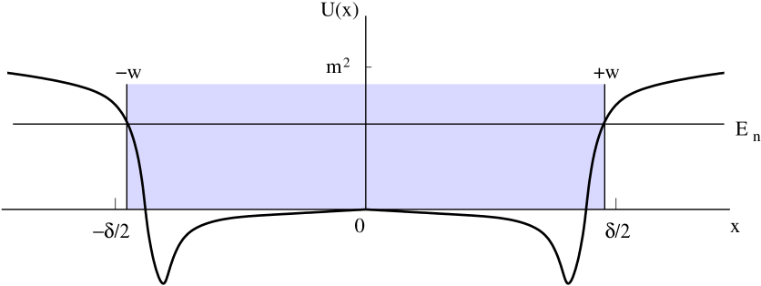
Figure 4: Sketch of $U(x)$ together with energy level $E_{n}$. The shaded region is the interior of the square well potential, $U_{sq}$, that is used to find the approximate dependence of $E_{n}$ on $n$.

Appendix B Form of domain wall fluctuation potentials

Here we show all that all kink potentials ($U$) have the supersymmetric form. We know that every kink has a translation mode which does not change the energy. Therefore, the Schrodinger equation (Eq. ((2)) gives

$$U(x)=\frac{\psi_{t}^{\prime\prime}}{\psi_{t}}$$ (64)

where $\psi_{t}(x)$ is the translation mode. This form of $U(x)$ can be rewritten as:

$$U(x)=f^{\prime}+f^{2}$$ (65)

where $f=[\ln(\psi_{t})]^{\prime}$, and hence $U$ is of the supersymmetric form (Eq. (11)) RodFilVai98 .

This argument can also be extended to higher dimensions with derivatives replaced by higher dimensional derivatives. Then we find:

$$U={\bf\nabla}\cdot{\bf f}+{\bf f}^{2}$$ (66)

where ${\bf f}({\bf x})={\bf\nabla}(\ln\psi_{t})$ is a vector valued function and $\psi_{t}({\bf x}$ is a translation mode. The Hamiltonian is:

$$H={\bf A}^{+}\cdot{\bf A}$$ (67)

where

$${\bf A}=-{\bf\partial}+{\bf f}$$ (68)

If $\psi$ is a multi-component scalar field, or a collection of several scalar and gauge field fluctuations, in several dimensions, there are circumstances in which $U$ is still supersymmetric. Label the many components of $\psi$ by the index $i$. So $\psi$ may be thought of as a column vector with components $\psi_{i}$. Now in higher dimensions, there will be several zero modes. For example, translations along any dimension will be a zero mode. So label the zero modes by the index $a$ and denote the translation modes by $\xi^{a}$. Then consider the matrix ${\bf M}$ whose components are $\xi^{a}_{i}$. We can show that $U$ is supersymmetric if we assume that ${\bf M}$ is a square matrix that is invertible. This follows because now:

$$[-{\bf\nabla}^{2}+U({\bf x})]{\bf M}=0$$ (69)

($U$ itself is a matrix potential.) Then it is easy to show that

$$U({\bf x})={\bf\nabla}\cdot{\bf F}+{\bf F}^{2}$$ (70)

where

$${\bf F}=({\bf\nabla}{\bf M}){\bf M}^{-1}$$ (71)

Appendix C Spectral properties of bound states in 1+1 dimensions

We now find the connection between the shape of the potential and the dependence of the $n^{th}$ eigenvalue, $E_{n}$, on $n$ for the specific class of potentials:

$$U(x)=a|x|^{b}$$ (72)

where $a$ and $b$ are parameters.

We use the WKB approximation Gri95 . The quantization condition for a particle of mass $\mu=1/2$ in the potential $U(x)$ is

$$\int_{-w(E_{n})}^{+w(E_{n})}dx\sqrt{E_{n}-U(x)}=n$$ (73)

where $E_{n}$ stands for $\omega_{n}^{2}$ in the notation of Sec. II. Inserting the class of potentials in Eq. (72), we find:

$$E_{n}\propto n^{2b/(b+2)}$$ (74)

Next we conside the WKB method in the context of the potential $U(x)$ redrawn here in Fig. 4.

Now,

$$n = \int_{-w(E_{n})}^{+w(E_{n})}dx\sqrt{E_{n}-U(x)}$$ (75)

$$= \int_{-w(E_{n})}^{+w(E_{n})}dx\sqrt{(E_{n}-U_{sq})-(U-U_{sq})}$$

$U_{sq}$ denotes the infinite square well potential of width $2w(E_{n})$ (see Fig. 4). Our assumption is that the dominant contribution to the integral comes from the $E_{n}-U_{sq}$ term and that the $U(x)-U_{sq}$ term can be ignored. Then the integral is trivial to do, resulting in $n=\sqrt{E_{n}}2w(E_{n})$. Now $2w(E_{n})\sim\delta$. Therefore $E_{n}\sim n^{2}$.

If $E_{n}$ is very small, our assumption that $U(x)-U_{sq}$ can be ignored will not hold. For reasonably large $E_{n}$ we can expect it to hold, though $E_{n}$ should still be much smaller than $m^{2}$ – the asymptotic value of $U$ – so that the finite depth of the well does not play a role.