Abstract

A cross between two well-known integrable multi-particle dynamics, an affine Toda molecule and a Sutherland system, is introduced for any affine root system. Though it is not completely integrable but partially integrable, or quasi exactly solvable, it inherits many remarkable properties from the parents. The equilibrium position is algebraic, i.e. proportional to the Weyl vector. The frequencies of small oscillations near equilibrium are proportional to the affine Toda masses, which are essential ingredients of the exact factorisable S-matrices of affine Toda field theories. Some lower lying frequencies are integer times a coupling constant for which the corresponding exact quantum eigenvalues and eigenfunctions are obtained. An affine Toda-Calogero system, with a corresponding rational potential, is also discussed.

1 Introduction

Calogero-Moser systems and (affine) Toda molecules are best known examples of integrable/solvable many-particle dynamics on a line which are based on root systems. The original Toda model [1] and the Calogero [2] and the Sutherland [3] models are based on the $A_{r}$ root system which correspond to the Lie algebra $\mathfrak{su}(r+1)$. Later integrable Toda [4, 5] and Calogero-Moser (C-M) [6, 5, 7, 8, 9] systems are formulated for any root system. The potentials of Toda systems are exponential functions of the coordinates, whereas those of Calogero-Moser systems are rational $1/q^{2}$, trigonometric $1/\sin^{2}q$, hyperbolic $1/\sinh^{2}q$ and elliptic $\wp(q)$ functions, in which $\wp$ is Weierstrass function and $q$ denotes the coordinates generically. In the C-M systems, the elliptic potentials are the most general ones and the rest (trigonometric, hyperbolic and rational) is obtained by various degeneration. In fact, a Toda molecule is obtained from an elliptic C-M system by a special limiting procedure [10, 11, 12]. While the potential of a C-M system depends on all (positive) roots, that of an (affine) Toda system contains (affine) simple roots only. For the $A$-type root systems the above feature is usually referred to that the C-M potential gives a pair-wise interactions and the Toda potential is of the nearest neighbour interaction type and the affine simple root corresponds to a periodic boundary condition.

In this paper we will present two new types of multi-particle dynamics related to any root system. Roughly speaking each could be considered as a cross between an (affine) Toda molecule and a C-M system. The first, to be tentatively called an (affine) Toda-Sutherland system, has trigonometric potentials $1/\sin^{2}q$ and depends on the (affine) simple roots only. The second, to be tentatively referred to as an (affine) Toda-Calogero system, has rational potentials $1/q^{2}$ plus a harmonic confining potential $q^{2}$ and depends on the (affine) simple roots only. The former has much richer structure than the latter and in this paper we mainly discuss the affine Toda-Sutherland systems. We do not think that they are integrable, either at the classical or the quantum level. But they have many remarkable features as shown in some detail for the systems based on the $A$-type root systems [13, 14, 15]. Their potentials have the nearest and next-to-nearest neighbour interactions, in contrast to the nearest neighbour interactions of the (affine) Toda molecule. These dynamical systems exhibit a behaviour intermediate to regular and chaotic. Like the C-M systems, these multi-particle dynamics are closely related to random matrix theory [13].

At the classical level, the frequencies of small oscillations at equilibrium [16] of an affine Toda-Sutherland system have exactly the same pattern as those of the affine Toda molecule based on the same root system. Let us point out that the pattern of the frequencies of small oscillations at equilibrium of an affine Toda molecule, or the so-called affine Toda masses appearing in the affine Toda field theory in $1+1$ dimensions [17], are the essential ingredient for its exact factorisable $S$-matrices. At the quantum level, most (but not all) of the multi-particle systems discussed in this paper are Quasi Exactly Solvable (QES) [18, 19]. That is, on top of the ground state eigenfunctions, a certain small number of eigenvalues and eigenfunctions are obtained exactly. The mechanism for QES seems very different from that of known ones [18, 19, 20].

This paper is organised as follows. In section 2, the salient features of affine Toda molecules are reviewed with a brief summary of roots and weights as essential ingredients. Section 3 is the main body of the paper. In section 3.1 we obtain the frequencies of small oscillations for Toda-Sutherland systems based on affine root systems. For these multiparticle systems we present some exact eigenvalues and eigenfunctions in section 3.2. They correspond to the low lying integer (times a coupling constant) frequencies of the small oscillations at equilibrium [16, 21]. In section 4 the affine Toda-Calogero systems are briefly discussed. The final section is reserved for summary and comments. In this paper we adopt the convention that $\hbar=1$ and do not show the dependence on the Planck’s constant.

2 Affine Toda molecule

The dynamical variables of a classical (quantum) multi-particle system to be discussed in this paper, an (affine) Toda molecule, a C-M system, an (affine) Toda-Sutherland system and an (affine) Toda-Calogero system, are the coordinates $\{q_{j}|\,j=1,\ldots,r\}$ and their canonically conjugate momenta $\{p_{j}|\,j=1,\ldots,r\}$, with the Poisson bracket (Heisenberg commutation) relations:

$$\{q_{j},p_{k}\} = \delta_{j\,k},\qquad\{q_{j},q_{k}\}=\{p_{j},p_{k}\}=0,$$

$$\ [q_{j},p_{k}] = i\delta_{j\,k},\qquad[q_{j},q_{k}]=[p_{j},p_{k}]=0.$$

These will be denoted by vectors in $\mathbf{R}^{r}$

$$q=(q_{1},\ldots,q_{r}),\qquad p=(p_{1},\ldots,p_{r}),$$

in which $r$ is the number of particles and it is also the rank of the underlying root system $\Delta$.

2.1 Roots and weights

Let $\Pi$ be the set of simple roots of $\Delta$:

$$\Pi=(\alpha_{1},\alpha_{2},\ldots,\alpha_{r}).$$ (2.1)

Any positive roots in $\Delta$ can be expressed as a linear combination of the simple roots with non-negative integer coefficients

$$\alpha=\sum_{j=1}^{r}m_{j}\alpha_{j},\qquad m_{j}\in\mathbb{Z}_{+},\quad\forall\alpha\in\Delta_{+}.$$ (2.2)

In the case of simply laced root systems ($A$, $D$, $E$) all the roots have the same length. We adopt the convention $\alpha^{2}=\alpha\cdot\alpha=2$. In the case of non-simply laced root systems ($B$, $C$, $F_{4}$, $G_{2}$), there are long roots and short roots. We adopt the convention $\alpha_{L}^{2}=2$ except for the $C$-series of the root system in which we adopt $\alpha_{S}^{2}=2$. Since $\Delta$ is a finite set, there exists an element $\alpha_{h}$ for which $\sum_{j=1}^{r}m_{j}$ is the maximum in $\Delta_{+}$. We call it the highest root and write it

$$\alpha_{h}=\sum_{j=1}^{r}n_{j}\alpha_{j},\qquad n_{j}\in\mathbb{Z}_{+}.$$ (2.3)

For the non-simply laced root systems, the highest roots are always long. We also introduce highest short root and denote it in the same way as (2.3) to avoid duplicating many formulas.

The positive integers $\{n_{j}\}$ are called Dynkin-Kac labels. We define the affine simple root $\alpha_{0}$ as the lowest (short) root, that is the negative of the highest (short) root:

$$\alpha_{0}=-\alpha_{h}=-(\sum_{j=1}^{r}n_{j}\alpha_{j}).$$ (2.4)

The above relationship can be rewritten in a symmetrical way:

$$\sum_{j=0}^{r}n_{j}\alpha_{j}=0,\quad n_{0}\equiv 1.$$ (2.5)

We call $\Pi_{0}$ the set of affine simple roots:

$$\Pi_{0}=\alpha_{0}\cup\Pi=(\alpha_{0},\alpha_{1},\ldots,\alpha_{r}),$$ (2.6)

which specifies the affine Lie algebra, to be denoted as $A_{r}^{(1)}$, $E_{6}^{(2)}$, $D_{4}^{(3)}$, etc. It has the necessary and sufficient information for defining affine Toda molecule (and its field theory version, the affine Toda field theory [17], too).

The fundamental weights $\{\lambda_{j}\}$ are the dual to the simple roots:

$$\alpha_{j}^{\vee}\cdot\lambda_{k} = \delta_{jk},\quad\alpha_{j}^{\vee}\equiv{2\alpha_{j}\over{\alpha_{j}^{2}}},\quad j=1,\ldots,r,$$ (2.7)

$$\alpha_{j}\cdot\lambda_{j}^{\vee} = \delta_{jk},\quad\lambda_{j}^{\vee}\equiv{2\over{\alpha_{j}^{2}}}\lambda_{j},\quad j=1,\ldots,r.$$ (2.8)

The equation (2.7) defines $\{\lambda_{j}\}$ and (2.8) defines $\{\lambda_{j}^{\vee}\}$ in turn. Next we define $\varrho$:

$$\varrho\equiv\sum_{j=1}^{r}\lambda_{j}^{\vee},$$ (2.9)

which is essentially the Weyl vector having the following properties

$$\alpha_{j}\cdot\varrho = 1,\qquad j=1,\ldots,r,$$ (2.10)

$$\alpha_{0}\cdot\varrho = -(\sum_{j=1}^{r}n_{j}\alpha_{j})\cdot\varrho=-(\sum_{j=1}^{r}n_{j})=-(h-1),$$ (2.11)

in which $h$ is the (dual) Coxeter number:

$$h\equiv\sum_{j=0}^{r}n_{j}=1+\sum_{j=1}^{r}n_{j}.$$ (2.12)

2.2 Hamiltonian, equilibrium position and frequencies of small oscillations

The Hamiltonian of the affine Toda molecule based on the set of affine simple roots $\Pi_{0}$ is

$$H = {1\over 2}p^{2}+V(q),$$ (2.13)

$$V(q) = {1\over{\beta^{2}}}\sum_{j=0}^{r}n_{j}e^{\beta\alpha_{j}\cdot q},$$ (2.14)

in which $\beta\in\mathbf{R}$ is the coupling constant. Note that all the particle masses are the same and normalised to unity. The potential $V(q)$ has a minimum (equilibrium point) at $q=0$ as

$$V(q)={h\over{\beta^{2}}}+{1\over{\beta}}(\sum_{j=0}^{r}n_{j}\alpha_{j})\cdot q+{1\over 2}\sum_{j=0}^{r}\sum_{k,l}^{r}n_{j}(\alpha_{j})_{k}(\alpha_{j})_{l}q_{k}q_{l}+o(q^{3}).$$ (2.15)

Here, $(\alpha_{j})_{k}$ is the $k$-th component of the (affine) simple root $\alpha_{j}$. The linear term vanishes due to (2.5) and the constant term is proportional to the Coxeter number $h$ given by (2.12).

The symmetric matrix $M$

$$M_{kl}=\sum_{j=0}^{r}n_{j}(\alpha_{j})_{k}(\alpha_{j})_{l},\qquad\mbox{or}\qquad M=\sum_{j=0}^{r}n_{j}\alpha_{j}\otimes\alpha_{j},$$ (2.16)

is called affine Toda mass matrix. Its eigenvalues

$$\mbox{Spec}(M)=\left\{m_{1}^{2},m_{2}^{2},\ldots,m_{r}^{2}\right\},\quad m_{j}>0.$$ (2.17)

are called affine Toda masses (squared). The set $\left\{m_{1},m_{2},\ldots,m_{r}\right\}$ gives $r$ (angular) frequencies of small oscillations at the equilibrium $q=0$. The above Hamiltonian (2.13)-(2.14) is completely integrable and classical Lax pair is known for all the affine simple root systems. This is a periodic Toda lattice if $\Pi_{0}$ is for $A_{r}^{(1)}$.

3 Affine Toda-Sutherland systems

The multi-particle dynamics with nearest and next-to-nearest trigonometric interactions introduced in [13, 14] can be called affine Toda-Sutherland model based on $A_{r}^{(1)}$. They can be generalised to any root system as follows.

Given an affine root system $\Pi_{0}$, let us introduce a prepotential $W$

$$W(q)=\beta\sum_{j=0}^{r}n_{j}\log|\sin(\alpha_{j}\cdot q)|,$$ (3.1)

in which $\beta\in\mathbf{R}_{+}$ is a positive coupling constant and $\{n_{j}\}$ are the Dynkin-Kac labels for $\Pi_{0}$. This leads to the Hamiltonians with the classical and quantum potentials $V_{C}$ and $V_{Q}$ as [9]

$$H_{C} = {1\over 2}p^{2}+V_{C}(q),\qquad V_{C}(q)={1\over 2}\sum_{j=1}^{r}\left({\partial W\over{\partial q_{j}}}\right)^{2},$$ (3.2)

$$H_{Q} = {1\over 2}p^{2}+V_{Q}(q),\qquad V_{Q}(q)={1\over 2}\sum_{j=1}^{r}\left[\left({\partial W\over{\partial q_{j}}}\right)^{2}+{\partial^{2}W\over{\partial q_{j}^{2}}}\right].$$ (3.3)

Again note that all the particle masses are the same and normalised to unity. Explicitly $V_{Q}$ reads

$$V_{Q} = {1\over 2}\sum_{j=0}^{r}{\beta n_{j}(\beta n_{j}-1)\alpha_{j}^{2}\over{\sin^{2}(\alpha_{j}\cdot q)}}+\beta^{2}\sum_{j<k}n_{j}n_{k}\alpha_{j}\cdot\alpha_{k}\cot(\alpha_{j}\cdot q)\cot(\alpha_{k}\cdot q)-E_{0},$$ (3.4)

$$E_{0} = {\beta^{2}\over 2}\sum_{j=0}^{r}n_{j}^{2}\alpha_{j}^{2},$$ (3.5)

in which the constant part $E_{0}$ can be considered as the ground state energy. The extended Dynkin diagram of $\Pi_{0}$ encodes all the necessary information $\{\alpha_{j}^{2}\}$, $\{\alpha_{j}\cdot\alpha_{k}\}$ and $\{n_{j}\}$ to determine $V_{Q}$. See [9, 16, 21] for the formulation of Hamiltonian dynamics in terms of a prepotential and the frequencies of small oscillations at equilibrium. The corresponding ground state wavefunction is

$$H_{Q}\psi_{0}=0,\qquad\psi_{0}(q)=e^{W(q)}=\prod_{j=0}^{r}|\sin(\alpha_{j}\cdot q)|^{\beta n_{j}}.$$ (3.6)

In contrast to the Calogero-Moser systems [7, 8], the prepotential (3.1), potential (3.3) and thus the Hamiltonian are not Weyl-invariant. For simplicity we consider the configuration space in the principal Weyl alcove:

$$PW_{T}=\{q\in{\bf R}^{r}|\ \alpha\cdot q>0,\quad\alpha\in\Pi,\quad\alpha_{h}\cdot q<\pi\},$$ (3.7)

where $\alpha_{h}$ is the highest root. (Due the non-invariance under the Weyl group, theories with different configuration spaces are physically different. For example, they have different (non-equivalent) equilibrium positions.)

For the simplest affine Lie algebra of $A_{r}^{(1)}$ the quantum Hamiltonian reads

$$H_{Q} = {1\over 2}p^{2}+\beta(\beta-1)\sum_{j=1}^{r+1}{1\over{\sin^{2}(q_{j}-q_{j+1})}}$$ (3.8)

$$\hskip 56.9055pt-\beta^{2}\sum_{j=1}^{r+1}\cot(q_{j-1}-q_{j})\cot(q_{j}-q_{j+1})-\beta^{2}(r+1).$$

This has the nearest and next-to-nearest neighbour interactions [13, 14]. The $B$, $BC$ and $D$ models in [13, 14, 15] are different from those in this paper.

3.1 Classical equilibrium

The equilibrium point ($\bar{q}$) of the classical Hamiltonian of the affine Toda-Sutherland system

$$H = {1\over 2}p^{2}+V_{C}(q),\quad V_{C}(q)={1\over 2}\sum_{j=1}^{r}\left({\partial W\over{\partial q_{j}}}\right)^{2},$$ (3.9)

$${\partial W\over{\partial q_{j}}} = \beta\sum_{k=0}^{r}n_{k}(\alpha_{k})_{j}\cot[\alpha_{k}\cdot q],\quad j=1,\ldots,r.$$ (3.10)

has a very intuitive characterisation. It is proportional to the Weyl vector $\varrho$ (2.9), $\bar{q}\propto\varrho$, the fundamental quantity of the Lie algebra. This is much simpler than the cases in the Calogero as well as Sutherland systems in which $\bar{q}$ correspond to the zeros of certain polynomials, i.e. the Hermite, Laguerre, Chebyshev and Jacobi polynomials for classical root systems [22, 16]. Since [16, 21]

$${\partial W(\bar{q})\over{\partial q_{j}}}=0,\quad j=1,\ldots,r\quad\Rightarrow\quad{\partial V_{C}(\bar{q})\over{\partial q_{l}}}=\sum_{j=1}^{r}{\partial^{2}W(\bar{q})\over{\partial q_{j}\partial q_{l}}}{\partial W(\bar{q})\over{\partial q_{j}}}=0,$$ (3.11)

the equilibrium is achieved at the point $\bar{q}$ where all $\partial W/\partial q_{j}$ vanish, i.e. at the maximum of the ground state wavefunction. It is easy to see that

$$\bar{q}=c\varrho,\quad c:const.,$$ (3.12)

gives a solution. Using (2.9)–(2.11),

$$\alpha_{k}\cdot\bar{q}=\left\{\begin{array}[]{cl}c&k=1,\ldots,r,\\ -(h-1)c&k=0,\end{array}\right.$$ (3.13)

we obtain

$${\partial W(\bar{q})\over{\partial q_{j}}}=\beta\left(\cot(c)\sum_{k=1}^{r}n_{k}(\alpha_{k})_{j}-\cot[(h-1)c](\alpha_{0})_{j}\right).$$ (3.14)

For

$$c={\pi\over h},$$ (3.15)

$c\varrho$ is in the principal Weyl alcove (3.7) and

$$\cot[(h-1)c]=\cot(\pi-c)=-\cot(c).$$ (3.16)

Thus we find $\bar{q}=\pi\varrho/h$ is the equilibrium

$${\partial W(\bar{q})\over{\partial q_{j}}}=\beta\cot[{\pi\over h}]\left(\sum_{k=0}^{r}n_{k}\alpha_{k}\right)_{j}=0.$$ (3.17)

The equilibrium points are equally spaced for all the classical root systems. The situation is different for the exceptional root systems. The equilibrium point $\bar{q}=\pi\varrho/h$ is unique in the principle Weyl alcove (3.7).

The squared frequencies of small oscillations at equilibrium $\bar{q}$ are given by the eigenvalues of the matrix

$$\left.{\partial^{2}V_{C}(q)\over{\partial q_{j}\partial q_{k}}}\right|_{\bar{q}}=\sum_{j=1}^{r}\left.{\partial^{2}W(q)\over{\partial q_{j}\partial q_{l}}}\right|_{\bar{q}}\left.{\partial^{2}W(q)\over{\partial q_{l}\partial q_{k}}}\right|_{\bar{q}}=(\widetilde{W}^{2})_{jk}.$$ (3.18)

Thus the frequencies of small oscillations at equilibrium $\bar{q}$ are given by the eigenvalues of a symmetric matrix $\widetilde{W}$ defined by

$$\widetilde{W}_{jk}=-\left.{\partial^{2}W(q)\over{\partial q_{j}\partial q_{k}}}\right|_{\bar{q}}={\beta\over{\sin^{2}{\pi\over h}}}\sum_{l=0}^{r}n_{l}(\alpha_{l})_{j}(\alpha_{l})_{k}={\beta\over{\sin^{2}{\pi\over h}}}M_{jk},$$ (3.19)

in which matrix $M$ is the mass square matrix of the affine Toda molecule associated with the affine root system $\Pi_{0}$ defined in (2.16).

The frequencies (not frequencies squared) of small oscillations at equilibrium of affine Toda-Sutherland model are given up to the coupling constant $\beta$ by

$${1\over{\sin^{2}{\pi\over h}}}\left\{m_{1}^{2},m_{2}^{2},\ldots,m_{r}^{2}\right\},$$ (3.20)

in which $m_{j}^{2}$ are the affine Toda masses. In [17] it is shown that the vector $\mathbf{m}=(m_{1},\ldots,m_{r})$, if ordered properly, is the Perron-Frobenius eigenvector of the incidence matrix (the Cartan matrix) of the corresponding root system. Therefore there exists a one-to-one correspondence between the mass $m_{j}$ and a vertex (or the fundamental weight) of the Dynkin diagram. This fact will be important in the next subsection for the explicit construction of exact eigenvalues and eigenfunctions. In Table I we list the affine Toda masses and the Coxeter number $h$ for the classical untwisted affine Lie algebras, $A_{r}^{(1)}$, $B_{r}^{(1)}$, $C_{r}^{(1)}$, $D_{r}^{(1)}$, see [17]:

$\Pi_{0}$	$h$	affine Toda masses
I$A_{r}^{(1)}$	$r+1$	$m_{j}^{2}=4\sin^{2}({j\pi\over h}),\quad j=1,\ldots,r,$
I$B_{r}^{(1)}$	$2r$	$m_{j}^{2}=8\sin^{2}({j\pi\over h}),\quad j=1,\ldots,r-1,\quad m_{r}^{2}=2,$
I$C_{r}^{(1)}$	$2r$	$m_{j}^{2}=8\sin^{2}({j\pi\over h}),\quad j=1,\ldots,r,$
I$D_{r}^{(1)}$	$2(r-1)$	$m_{j}^{2}=8\sin^{2}({j\pi\over h}),\quad j=1,\ldots,r-2,\quad m_{r-1}^{2}=m_{r}^{2}=2.$

Table I: The Coxeter number $h$ and the affine Toda masses $m_{j}^{2}$

for classical untwisted affine Lie algebras.

Those for the exceptional affine Lie algebras $E_{r}^{(1)}$, $F_{4}^{(1)}$ and $G_{2}^{(1)}$ we refer to [17]. (The affine Toda masses for $E_{8}$ reported there need a factor 2.) The twisted affine Lie algebras, for example $D_{r+1}^{(2)}$, $E_{6}^{(2)}$, $D_{4}^{(3)}$, etc., which are characterised by the highest short roots, can also be obtained from untwisted affine Lie algebras by folding [17]. The affine Toda masses for the twisted affine Lie algebra are closely related to those of the original untwisted affine Lie algebra.

3.2 Quantum eigenfunctions

Here we demonstrate that some of the quantum affine Toda-Sutherland (3.3) systems have a number of exact eigenvalues and eigenfunctions and thus they are partially integrable or quasi exactly solvable [18, 19]. These are usually a small number of lowest lying excited states. The occurrence of such exact states is strongly correlated with the appearance of the integer eigenvalues in the spectrum of the small oscillations near the classical equilibrium, as shown in the recent general theorems by Loris-Sasaki [21]. Let us express the eigenfunctions in product forms

$$\psi_{n}(q)=\phi_{n}(q)\psi_{0}(q),\quad n=0,1,\ldots,\qquad\phi_{0}\equiv 1,$$ (3.21)

in which $\phi_{n}$ obeys a simplified equation with the similarity transformed Hamiltonian $\tilde{H}$ [9]:

$$\tilde{H}\phi_{n} = E_{n}\phi_{n},$$ (3.22)

$$\tilde{H}=e^{-W}H_{Q}e^{W} = -{1\over 2}\triangle-\sum_{j=1}^{r}{\partial W\over{\partial q_{j}}}{\partial\over{\partial q_{j}}},\quad\triangle\equiv\sum_{j=1}^{r}{\partial^{2}\over{\partial q_{j}^{2}}}.$$ (3.23)

3.2.1 $A_{r}^{(1)}$

In this case the spectrum of the small oscillations, up to the coupling constant $\beta$ is easily read from Table I:

$$4\left\{1,\ldots,\sin^{2}(j\pi/(r+1))/\sin^{2}(\pi/(r+1)),\ldots,1\right\}.$$ (3.24)

Reflecting the left-right mirror symmetry $j\leftrightarrow r+1-j$ of the Dynkin diagram Fig.1, the spectrum is doubly degenerate except for the possible singlet at the middle point $j=(r+1)/2$ for odd $r$.

The doubly degenerate integer eigenvalues 4 correspond to the two end points of the $A_{r}^{(1)}$ Dynkin diagram, Fig.1. They correspond to the fundamental vector and conjugate vector representations and to the eigenfunctions:

$$\mathbf{v}=\sum_{j=1}^{r+1}e^{2iq_{j}},\quad\bar{\mathbf{v}}=\sum_{j=1}^{r+1}e^{-2iq_{j}}.$$ (3.25)

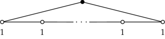
Figure 1: $A_{r}^{(1)}$ Dynkin diagram with the numbers $n_{j}$ attached. The black spot is the affine simple root.

It is easy to verify

$$\tilde{H}\mathbf{v}=(4\beta+2)\mathbf{v},\quad\tilde{H}\bar{\mathbf{v}}=(4\beta+2)\bar{\mathbf{v}},\quad-{1\over 2}\triangle\mathbf{v}=2\mathbf{v},\quad-{1\over 2}\triangle\bar{\mathbf{v}}=2\bar{\mathbf{v}}.$$ (3.26)

The affine simple root corresponds to the adjoint representation. Let us define

$$\phi_{a}=\phi_{v\bar{v}}+2\beta/(1+2\beta),\quad\phi_{v\bar{v}}=\sum_{j\neq k}e^{2i(q_{j}-q_{k})}.$$ (3.27)

It is easy to show

$$\tilde{H}\phi_{a}=(8\beta+4)\phi_{a},$$ (3.28)

in which $8\beta$ is simply a sum of $4\beta$ for $\mathbf{v}$ and another $4\beta$ for $\bar{\mathbf{v}}$ in (3.25).

For $A_{2}^{(1)}$, the system is identical with the $A_{2}$ Sutherland model. For the special case of $A_{3}^{(1)}$, the above spectrum (3.24) is $\{4,8,4\}$. We find another complex eigenfunction with the classical eigenvalue $8\beta$

$$\phi_{t}=\sum_{j=1}^{4}e^{4iq_{j}}-e^{2i(q_{1}+q_{2}+q_{3}+q_{4})}\sum_{j=1}^{4}e^{-4iq_{j}},\quad\tilde{H}\phi_{t}=(8\beta+8)\phi_{t}.$$ (3.29)

3.2.2 $D_{r}^{(1)}$

The spectrum of the small oscillations, up to the coupling constant $\beta$ is easily read from Table I:

$$8\left\{1,\ldots,\sin^{2}(j\pi/2(r-1))/\sin^{2}(\pi/2(r-1)),\ldots\right\},\quad\mbox{and}\quad 2/\sin^{2}(\pi/2(r-1))[2],$$ (3.30)

in which the two degenerate frequencies at the end correspond to the spinor and anti-spinor weights at the right end of the $D_{r}^{(1)}$ Dynkin diagram in Fig.2.

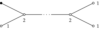
Figure 2: $D_{r}^{(1)}$ Dynkin diagram with the numbers $n_{j}$ attached. The black spot is the affine simple root.

For $r\geq 5$ these eigenvalues are greater than 8, which belongs to the vector weights at the left end of the Dynkin diagram Fig.2. The set of vector weights is $\mathbf{V}=\{\pm\mathbf{e}_{j}|j=1,\ldots,r\}$. Let us introduce the corresponding wavefunctions

$$\phi_{\mathbf{V}}=\sum_{\mu\in\mathbf{V}}e^{2i\mu\cdot q}=2\sum_{j=1}^{r}\cos 2q_{j}.$$ (3.31)

However, it is not an eigenfunction

$$\tilde{H}\phi_{\mathbf{V}}=(8\beta+2)\phi_{\mathbf{V}}-8\beta(\cos 2q_{1}+\cos 2q_{r}),\quad-{1\over 2}\triangle\phi_{\mathbf{V}}=2\phi_{\mathbf{V}}.$$ (3.32)

This would give an eigenfunction in a theory if $q_{1}$ and $q_{r}$ are constrained to 0; $q_{1}\equiv 0\equiv q_{r}$. If this restriction is made in the prepotential $W$ of $D_{r}^{(1)}$ theory together with $2\beta\to\beta$ (and $r\to r+2$), it gives the prepotential of the $D_{r+1}^{(2)}$ to be discussed shortly in section 3.2.3. The corresponding eigenfunction is (3.38). The formula (3.32) also ‘explains’ the non-existence of the corresponding eigenfunction in $B_{r}^{(1)}$ theory, which is obtained by restriction $q_{r}\equiv 0$ (together with $r\to r+1$).

For the special case of $r=3$ the eigenvalues for the spinor and anti-spinor weights are lower than that of the vector weights. We find several lower lying eigenstates:

$$D_{3}^{(1)}:$$

$$\phi_{s1} = \sin q_{1}\sin q_{2}\sin q_{3},\qquad\qquad\ \,\tilde{H}\phi_{s1}=(4\beta+3/2)\phi_{s1},$$ (3.33)

$$\phi_{s2} = \cos q_{1}\cos q_{2}\cos q_{3},\qquad\qquad\tilde{H}\phi_{s2}=(4\beta+3/2)\phi_{s2},$$ (3.34)

$$\phi_{ss} = \sin 2q_{1}\sin 2q_{2}\sin 2q_{3},\qquad\quad\tilde{H}\phi_{ss}=(8\beta+6)\phi_{ss},$$ (3.35)

$$\phi_{2} = \cos 2q_{1}\cos 2q_{2}+\cos 2q_{1}\cos 2q_{3}+\cos 2q_{2}\cos 2q_{3}+2\beta/(1+2\beta),$$ (3.36)

$$\hskip 139.4185pt\tilde{H}\phi_{2}=(8\beta+4)\phi_{2}.$$

These are closely related to the eigenfunctions of the $A_{r}^{(1)}$, (3.26), (3.27) and (3.29) since $A_{3}^{(1)}\cong D_{3}^{(1)}$.

3.2.3 $D_{r+1}^{(2)}$

The extended Dynkin diagram of $D_{r+1}^{(2)}$, Fig.3, can be obtained from that of $B_{r+1}^{(1)}$ by folding the left ‘fish tail’ containing the affine simple root. Then $B_{r+1}^{(1)}$ is obtained from $D_{r+2}^{(1)}$ by folding the right ‘fish tail’ corresponding to the spinor and anti-spinor weights. The affine simple root of $D_{r+1}^{(2)}$ is the ‘lowest short root’ of $B_{r}$. In this case the spectrum of the small oscillations, up to the coupling constant $\beta$ is:

$$4\left\{1,\ldots,\sin^{2}(j\pi/(r+1))/\sin^{2}(\pi/(r+1)),\ldots\right\}.$$ (3.37)

Figure 3: $D_{r+1}^{(2)}$ Dynkin diagram with the numbers $n_{j}$ attached. The black spot is the affine simple root.

The lowest eigenvalue is an integer 4 (times $\beta$) which corresponds to the vector weights of $B_{r}$, the leftmost white vertex in Fig.3. The set of vector weights is $\mathbf{V}=\{\pm\mathbf{e}_{j}|j=1,\ldots,r\}$. Let us introduce the corresponding wavefunctions

$$\phi=\phi_{\mathbf{V}}+{2\beta/(1+2\beta)},\quad\phi_{\mathbf{V}}=\sum_{\mu\in\mathbf{V}}e^{2i\mu\cdot q}=2\sum_{j=1}^{r}\cos 2q_{j}.$$ (3.38)

It is easy to see

$$\tilde{H}\phi=(4\beta+2)\phi,\quad-{1\over 2}\triangle\phi_{\mathbf{V}}=2\phi_{\mathbf{V}}.$$ (3.39)

3.2.4 $C_{r}^{(1)}$

The spectrum of the small oscillations, up to the coupling constant $\beta$ is easily read from Table I:

$$8\left\{1,\ldots,\sin^{2}(j\pi/(2r))/\sin^{2}(\pi/(2r)),\ldots\right\}.$$ (3.40)

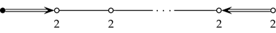
Figure 4: $C_{r}^{(1)}$ Dynkin diagram with the numbers $n_{j}$ attached. The black spot is the affine simple root.

The lowest eigenvalue is an integer 8 (times $\beta$) which belongs to the vector weight of $C_{r}$, corresponding to the leftmost white vertex of Fig.4. The set of vector weights is $\mathbf{V}=\{\pm\mathbf{e}_{j}|j=1,\ldots,r\}$. Let us introduce the corresponding wavefunctions

$$\phi_{\mathbf{V}}=\sum_{\mu\in\mathbf{V}}e^{2i\mu\cdot q}=2\sum_{j=1}^{r}\cos 2q_{j}.$$ (3.41)

It is easy to see

$$\tilde{H}\phi_{\mathbf{V}}=(8\beta+2)\phi,\quad-{1\over 2}\triangle\phi_{\mathbf{V}}=2\phi_{\mathbf{V}}.$$ (3.42)

As is well known $C_{r}^{(1)}$ is obtained from $A_{2r-1}^{(1)}$ by folding. The above eigenfunction originates from (3.25).

3.2.5 $A_{2r}^{(2)}$

This is also called a $BC_{r}$ root system, which is obtained by adding the affine root of $C_{r}^{(1)}$ to the set of simple roots of $B_{r}$. The spectrum of the small oscillations, up to the coupling constant $\beta$ is:

$$8\left\{1,\ldots,\sin^{2}(j\pi/(2r+1))/\sin^{2}(\pi/(2r+1)),\ldots\right\}.$$ (3.43)

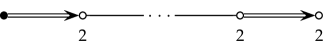
Figure 5: $A_{2r}^{(2)}$ Dynkin diagram with the numbers $n_{j}$ attached. The black spot is the affine simple root.

The lowest eigenvalue is an integer 8 (times $\beta$) which corresponds to the vector weight of $B_{r}$, $\mathbf{V}=\{\pm\mathbf{e}_{j}|j=1,\ldots,r\}$. Let us introduce the corresponding wavefunctions

$$\phi=\phi_{\mathbf{V}}+{4\beta/(1+4\beta)},\quad\phi_{\mathbf{V}}=\sum_{\mu\in\mathbf{V}}e^{2i\mu\cdot q}=2\sum_{j=1}^{r}\cos 2q_{j}.$$ (3.44)

It is easy to see

$$\tilde{H}\phi=(8\beta+2)\phi,\quad-{1\over 2}\triangle\phi_{\mathbf{V}}=2\phi_{\mathbf{V}}.$$ (3.45)

As in the $D_{r+1}^{(2)}$ case (3.38), the eigenfunction (3.44) has a constant part. This is related to the fact that the vector representation of $B_{r}$ contains a zero weight. In contrast the vector representation of $C_{r}$ does not contain a zero weight and the corresponding eigenfunction (3.41) does not have a constant part. This also explains that the eigenfunctions corresponding to the vector and conjugate vector representations (3.26) do not have a constant part, whereas that corresponding to the adjoint representation (3.27) has a constant part. The adjoint representation has a rank number of zero weights.

3.2.6 Exceptional affine Lie algebras

For $E_{6}^{(1)}$, $E_{7}^{(1)}$, $E_{8}^{(1)}$ and $F_{4}^{(1)}$ none of the frequencies of (3.20) are integers. The $G_{2}^{(1)}$ case, which is obtained from $D_{4}^{(1)}$ by three-fold folding, has two integer eigenvalues $\left\{8,24\right\}$ inherited from $D_{4}^{(1)}$. As shown in 3.2.2, we found no exact eigenfunctions for $D_{r}^{(1)}$ and $D_{4}^{(1)}$. Therefore we do not expect any exact eigenfunctions for the exceptional affine Toda-Sutherland systems and we have got none.

3.3 Comments on non-affine Toda-Sutherland systems

In the Toda molecule (Toda field theory) interactions, the affine simple root $\alpha_{0}$ plays an essential role for the existence of an equilibrium. However, with $1/\sin^{2}q$ type interactions, an equilibrium is achieved without the affine simple root $\alpha_{0}$. This opens a way to consider (non-affine) Toda-Sutherland systems characterised by a prepotential

$$W(q)=\beta\sum_{\alpha\in\Pi}\log|\sin(\alpha\cdot q)|=\beta\sum_{j=1}^{r}\log|\sin(\alpha_{j}\cdot q)|.$$ (3.46)

Note that it does not contain the affine simple root $\alpha_{0}$ nor the Dynkin-Kac labels $\{n_{j}\}$. Since the highest root is not contained in the prepotential, the configuration space now is

$$PW_{N}=\{q\in{\bf R}^{r}|\ 0<\alpha\cdot q<\pi,\quad\alpha\in\Pi\}.$$ (3.47)

Finding the equilibrium position $\bar{q}$ of the classical potential is easy. It is again proportional to the Weyl vector $\varrho$ (2.9)

$$\bar{q}={\pi\over 2}\varrho,\quad\alpha_{j}\cdot\bar{q}={\pi\over 2},\quad\cot[\alpha_{j}\cdot\bar{q}]=0\quad\Rightarrow\left.{\partial W(q)\over{\partial q_{j}}}\right|_{\bar{q}}=0,\quad j=1,\ldots,r.$$ (3.48)

Due to the linear independence of the simple roots, this equilibrium is unique in the configuration space (3.47). The frequencies of small oscillations near the equilibrium are the eigenvalues of the matrix

$$\widetilde{W}_{jk} = -\left.{\partial^{2}W(q)\over{\partial q_{j}\partial q_{k}}}\right|_{\bar{q}}=\beta\sum_{l=1}^{r}(\alpha_{l})_{j}(\alpha_{l})_{k}=\beta\tilde{M}_{jk},$$ (3.49)

$$\tilde{M} = \sum_{j=1}^{r}\alpha_{j}\otimes\alpha_{j}.$$ (3.50)

For the simply laced root systems ($A$, $D$, $E$) the spectrum of $\tilde{M}$ is the same as the spectrum of the Cartan matrix $C_{jk}=2\alpha_{j}\cdot\alpha_{k}/\alpha_{k}^{2}$, $j,k\in\Pi$. There is a universal formula for the spectrum of $\tilde{M}$ for the $A$, $D$, $E$ series:

$$\mbox{Spec}(\tilde{M})=\{4\sin^{2}(e_{1}/2h),\ldots,4\sin^{2}(e_{r}/2h)\},\quad e_{1},\ldots,e_{r}:\mbox{exponents}.$$ (3.51)

The exponents of simply laced root systems are:

$\Delta$	$h$	exponents, $e_{1}$,…, $e_{r}$	$\Delta$	$h$	exponents, $e_{1}$,…, $e_{r}$
I$A_{r}$	$r+1$	1, 2, 3, …, $r$	$E_{6}$	$12$	1, 4, 5, 7, 8, 11
I$D_{r}$	$2r$	1, 3, 5,…, $2r-1$; $r-1$	$E_{7}$	$18$	1, 5, 7, 9, 11, 13, 17
			$E_{8}$	$30$	1, 7, 11, 13, 17, 19, 23, 29

Table II: The exponents $e_{j}$ for simply laced root systems.

For the $B$ series and $G_{2}$ we have

$$B_{r}:\ \mbox{Spec}(\tilde{M}) = \{4\sin^{2}(2j-1/2(2r+1))|j=1,\ldots,r\},$$ (3.52)

$$G_{2}:\ \mbox{Spec}(\tilde{M}) = \{(4-\sqrt{13})/3,(4+\sqrt{13})/3\},$$ (3.53)

and analytical formulas are not known for the entire spectrum of $\tilde{M}$ in $C_{r}$ and $F_{4}$.

Although some of the eigenfrequencies of the small oscillations near the classical equilibrium (3.51), (3.52) are integers, they are definitely not the lowest lying ones. According to the quantum-classical correspondence [21], we do not expect to find the exact eigenfunctions for the lowest lying states, which have non-integer eigenvalues. Thus it is highly unlikely that the eigenfunctions for the higher excited states, being orthogonal to all the lower lying ones, could be obtained exactly, even for the ones belonging to integer classical eigenvalues. In fact we have not been able to find any exact eigenfunctions for the (non-affine) Toda-Sutherland systems (3.46).

4 Affine Toda-Calogero systems

Like the affine Toda-Sutherland system, the affine Toda-Calogero system can be defined for any affine root system $\Pi_{0}$ (2.6). However, in many respects the affine Toda-Calogero systems have less remarkable properties than the affine Toda-Sutherland systems discussed in the preceding section. The equilibrium position $\bar{q}$ does not have a simple characterisation. Except for the systems based on the $A^{(1)}$ series, the small oscillations near the equilibrium do not have integer (times the coupling constant) eigenvalues other than 2, which is universal for all the potentials with quadratic plus inverse quadratic dependence on the coordinate $q$ [23].

The prepotential of the affine Toda-Calogero system is obtained from that of affine Toda-Sutherland system (3.1) by changing $\sin\alpha_{j}\cdot q\to\alpha_{j}\cdot q$ and adding a harmonic confining potential with (angular) frequency $\omega>0$:

$$W(q)=\beta\sum_{j=0}^{r}n_{j}\log|\alpha_{j}\cdot q|-{\omega\over 2}q^{2}.$$ (4.1)

Because of the singularity of the potential we restrict the configuration space to the principal Weyl chamber for simplicity:

$$PW=\{q\in{\bf R}^{r}|\ \alpha\cdot q>0,\quad\alpha\in\Pi\}.$$ (4.2)

(Due the non-invariance under the Weyl group, theories with different configuration spaces are physically different. For example, they have different (non-equivalent) equilibrium positions.) The classical and quantum Hamiltonians are given in terms of the prepotential $W$ by the same formulas (3.2) and (3.3). The classical equilibrium position $\bar{q}$ is determined by

$${\partial W(\bar{q})\over{\partial q_{k}}}=0,\quad k=1,\ldots,r\quad\Longleftrightarrow\quad\beta\sum_{j=0}^{r}{n_{j}\alpha_{j}\over{\alpha_{j}\cdot\bar{q}}}=\omega\bar{q}.$$ (4.3)

In contrast to the Calogero systems in which $\bar{q}$ corresponds to the zeros of classical polynomials, i.e. the Hermite and the Laguerre polynomials for the classical root systems [22, 16], the present case does not have such simple characterisation. The frequencies of small oscillations near the equilibrium are given by the eigenvalues of the matrix

$$\widetilde{W}=\mbox{Matrix}\left(-{\partial^{2}W(\bar{q})\over{\partial q_{j}\partial q_{k}}}\right).$$

We have evaluated $\bar{q}$ and $\widetilde{W}$ numerically for various affine root systems. We will discuss the systems based on the $A^{(1)}$ series in the section 4.1. In all the other cases the only integer (times $\omega$) eigenvalues of $\widetilde{W}$ is 2, which exists in all the cases based on any root system. In fact it is more universal and exists for all the potentials with quadratic ($q^{2}$) plus inverse quadratic dependence on the coordinate $q$ [23, 9] without any root or weight structure. This eigenvalue 2 gives rise to exact quantum eigenfunctions $\phi_{n}(q)$ which is proportional to the Laguerre polynomial [23, 9] in $q^{2}$:

$$\tilde{H}\phi_{n}(q)=2\omega n\phi_{n}(q),\qquad\phi_{n}(q)\propto L_{n}^{(E_{0}/\omega-1)}(\omega q^{2}),\quad n=1,2,\ldots,$$ (4.4)

in which $E_{0}=(\beta h+r/2)\omega$ is the ground state energy and $h$ is the Coxeter number (2.12). Let us emphasise that these quantum eigenfunctions are also universal in the above sense.

Here the similarity transformed Hamiltonian $\tilde{H}$ and the eigenfunctions $\{\phi_{n}(q)\}$ are defined in terms of the ground state wavefunction $\psi_{0}=e^{W}$ in the same formulas as before (3.21)–(3.23).

4.1 $A_{r}^{(1)}$

This theory and its possible generalisation have been discussed rather extensively by Khare and collaborators [13, 14, 15] with explicit forms of quantum eigenfunctions. These multi-particle dynamics have nearest and next-to-nearest interactions with rational $1/q^{2}$ plus $q^{2}$ potentials. Here we discuss the relationship between the exact eigenfunctions and their classical counterparts [21]. The $A_{2}^{(1)}$ affine Toda-Calogero system is identical with $A_{2}$ Calogero system. The spectrum of $\widetilde{W}$ for $A_{r}^{(1)}$, $r\geq 3$ has a form

$$\mbox{Spec}(\widetilde{W})=\omega\{1,2,3,*,\ldots\},$$ (4.5)

in which $*,\ldots$ denote non-integers greater than 3.

The interpretation of these three integer eigenvalues is quite clear. The lowest one corresponds to the elementary excitation of the center of mass coordinates $Q=q_{1}+\ldots+q_{r+1}$ and the quantum eigenfunction belonging to the eigenvalue $n\omega$ is essentially the Hermite polynomial of degree $n$ in $Q$. The eigenfunctions corresponding to the eigenvalue 2 are the Laguerre polynomials (4.4) mentioned above. Let us introduce the elementary symmetric polynomial of degree $k$ in $q_{1},\ldots,q_{r+1}$ [21]:

$$\prod_{j=1}^{r+1}(x+q_{j})=\sum_{k=0}^{r+1}S_{k}x^{r+1-k},\quad S_{0}=1,\quad S_{1}=q_{1}+\cdots+q_{r+1}\equiv Q.$$ (4.6)

Since $S_{k}$ is annihilated by the Laplacian, $\triangle S_{k}=0$, one finds easily the exact quantum eigenfunction $\phi_{3}$ corresponding to the integer eigenvalue 3 in (4.5):

$$\tilde{H}S_{3}=3\omega S_{3}+\beta(r-1)Q,\quad\tilde{H}\phi_{3}=3\omega\phi_{3},\quad\phi_{3}=S_{3}+{\beta(r-1)\over{2\omega}}Q.$$ (4.7)

5 Summary and comments

The affine Toda-Sutherland system is introduced for any affine root system as a cross between the affine Toda molecule and the Sutherland system. That is, the potential is trigonometric, $1/\sin^{2}q$, and the multi-particle interactions are governed by the affine simple roots only, in contrast to the entire set of roots in the Sutherland system. It has remarkable universal features. The classical equilibrium point is $\pi\varrho/h$ ($\varrho$: Weyl vector, $h$: Coxeter number) and the frequencies of small oscillations near the equilibrium are proportional to the corresponding affine Toda masses. In most cases based on classical affine Lie algebras, some low lying frequencies are integers (times a coupling constant). They give rise to exact quantum eigenvalues and eigenfunctions. The ground state eigenfunctions are always given explicitly. Thus the affine Toda-Sutherland systems provide examples of a new type of quasi exactly solvable multi-particle dynamics.

Affine Toda-Calogero systems with rational ($1/q^{2}$ plus $q^{2}$) potentials are found to be less remarkable than their trigonometric counterparts. They possess an infinite number of exact eigenvalues and eigenfunctions which are well known. We have shown that the affine Toda-Calogero systems based on $A^{(1)}$ series have three lowest frequencies $\omega$, $2\omega$ and $3\omega$ of small oscillations near the classical equilibrium. They all correspond to exact quantum eigenvalues and eigenfunctions.

It would be interesting to understand these ‘partially integrable’ affine Toda-Sutherland-Calogero systems from various points of view: relationship with the random matrix models, analysis from the regular and chaotic dynamics, etc.

In [13, 14, 15] many interesting multi-particle dynamics, rational and trigonometric, related to the root systems of $B_{r}$, $C_{r}$, $BC_{r}$ and $D_{r}$ were introduced. They resemble to our affine Toda-Sutherland and affine Toda-Calogero systems but they cannot be characterised in terms of affine simple roots. Unified understanding of these systems is wanted.

References

- [1] M. Toda, “Vibration of a chain with nonlinear interaction”, J. Phys. Soc. Jpn. 22 (1967) 431-436.
- [2] F. Calogero, “Solution of the one-dimensional -body problem with quadratic and/or inversely quadratic pair potentials”, J. Math. Phys. 12 (1971) 419-436.
- [3] B. Sutherland, “Exact results for a quantum many-body problem in one-dimension. II”, Phys. Rev. A5 (1972) 1372-1376.
- [4] B. Kostant, “The solution to a generalized Toda lattice and representation theory”, Adv. in Math. 34 (1979) 195–338.
- [5] M. A. Olshanetsky and A. M. Perelomov, “Classical integrable finite-dimensional systems related to Lie algebras”, Phys. Rep. C71 (1981), 314-400.
- [6] J. Moser, “Three integrable Hamiltonian systems connected with isospectral deformations”, Adv. Math. 16 (1975) 197-220; J. Moser, “Integrable systems of non-linear evolution equations”, in Dynamical Systems, Theory and Applications; J. Moser, ed., Lecture Notes in Physics 38 (1975), Springer-Verlag; F. Calogero, C. Marchioro and O. Ragnisco, “Exact solution of the classical and quantal one-dimensional many body problems with the two body potential ”, Lett. Nuovo Cim. 13 (1975) 383-387; F. Calogero, “Exactly solvable one-dimensional many body problems”, Lett. Nuovo Cim. 13 (1975) 411-416.
- [7] M. A. Olshanetsky and A. M. Perelomov, “Completely integrable Hamiltonian systems connected with semisimple Lie algebras”, Inventions Math. 37 (1976), 93-108.
- [8] E. D’Hoker and D. H. Phong, “Calogero-Moser Lax pairs with spectral parameter for general Lie algebras”, Nucl. Phys. B530 (1998) 537-610, hep-th/9804124; A. J. Bordner, E. Corrigan and R. Sasaki, “Calogero-Moser models I: a new formulation”, Prog. Theor. Phys. 100 (1998) 1107-1129, hep-th/9805106; “Generalized Calogero-Moser models and universal Lax pair operators”, Prog. Theor. Phys. 102 (1999) 499-529, hep-th/9905011.
- [9] A. J. Bordner, N. S. Manton and R. Sasaki, “Calogero-Moser models V: Supersymmetry and Quantum Lax Pair”, Prog. Theor. Phys. 103 (2000) 463-487, hep-th/9910033; S. P. Khastgir, A. J. Pocklington and R. Sasaki, “Quantum Calogero-Moser Models: Integrability for all Root Systems”, J. Phys. A33 (2000) 9033-9064, hep-th/0005277.
- [10] V. I. Inozemtsev, “The finite Toda lattices”, Comm. Math. Phys. 121 (1989) 628-638.
- [11] E. D’Hoker and D. H. Phong, “Calogero-Moser and Toda systems for twisted and untwisted affine Lie Algebras”, Nucl. Phys. B530 (1998) 611-640, hep-th/9804125.
- [12] S. P. Khastgir, R. Sasaki and K. Takasaki, “Calogero-Moser Models IV: Limits to Toda theory”, Prog. Theor. Phys. 102 (1999) 749-776, hep-th/9907102.
- [13] S. R. Jain and A. Khare, “An exactly solvable many-body problem in one dimension”, Phys. Lett. A262 (1999) 35-39; S. R. Jain, B. Grémaud and A. Khare, “Quantum modes on chaotic motion: Analytically exact results”, Phys. Rev. E66 (2002) 016216.
- [14] G. Auberson, S. R. Jain and A. Khare, “Off-diagonal long-range order in one-dimensional many-body problem”, Phys. Lett. A267 (2000) 293-295; “A class of N-body problems with nearest- and next-to-nearest neighbour interactions”, J. Phys. A34 (2001) 695-724, cond-mat/0004012.
- [15] M. Ezung, N. Gurappa, A. Khare and P. K. Panigrahi, “Algebraic study of quantum many-body systems with nearest and next-to-nearest neighbour long-range interactions,” cond-mat/0007005.
- [16] E. Corrigan and R. Sasaki, “Quantum vs classical integrability in Calogero-Moser systems”, J. Phys. A 35 (2002) 7017-7062, hep-th/0204039; S. Odake and R. Sasaki, “Polynomials associated with equilibrium positions in Calogero-Moser systems,” J. Phys. A 35 (2002) 8283-8314, hep-th/0206172; O. Ragnisco and R. Sasaki, “Quantum vs classical integrability in Ruijsenaars-Schneider systems”, Preprint YITP-03-09, hepth/0305120.
- [17] H. W. Braden, E. Corrigan, P. E. Dorey and R. Sasaki, “Affine Toda Field Theory and Exact S-Matrices,” Nucl. Phys. B 338 (1990) 689-746.
- [18] A. V. Turbiner, “Quasi-exactly-soluble problems and sl(2,R) algebra”, Comm. Math. Phys. 118 (1988) 467-474.
- [19] A. G. Ushveridze, “Qusi-exactly solvable models in quantum mechanics”, IOP Publishing, Bristol, (1994).
- [20] R. Sasaki and K. Takasaki, “Quantum Inozemtsev model, quasi-exact solvability and -fold supersymmetry”, J. Phys. A34 (2001) 9533-9553, [Erratum-ibid. A34 (2001) 10335], hep-th/0109008.
- [21] I. Loris and R. Sasaki, “Quantum vs classical mechanics: role of elementary excitations”, Kyoto preprint YITP-03-50, quant-ph/0308040; “Quantum & classical eigenfunctions in Calogero & Sutherland systems”, Kyoto preprint YITP-03-51, hep-th/0308052.
- [22] F. Calogero, “On the zeros of the classical polynomials”, Lett. Nuovo Cim. 19 (1977) 505-507; “Equilibrium configuration of one-dimensional many-body problems with quadratic and inverse quadratic pair potentials”, Lett. Nuovo Cim. 22 (1977) 251-253; “Eigenvectors of a matrix related to the zeros of Hermite polynomials”, Lett. Nuovo Cim. 24 (1979) 601-604; “Matrices, differential operators and polynomials”, J. Math. Phys. 22 (1981) 919-934.
- [23] P. J. Gambardella, “Exact results in quantum many-body systems of interacting particles in many dimensions with as the dynamical group”, J. Math. Phys. 16 1172-1187 (1975).