Integrable Structure of the Dirichlet Boundary Problem in Multiply-Connected Domains

We study the integrable structure of the Dirichlet boundary problem in two dimensions and extend the approach to the case of planar multiply-connected domains. The solution to the Dirichlet boundary problem in multiply-connected case is given through a quasiclassical tau-function, which generalizes the tau-function of the dispersionless Toda hierarchy. It is shown to obey an infinite hierarchy of Hirota-like equations which directly follow from properties of the Dirichlet Green function and from the Fay identities. The relation to multi-support solutions of matrix models is briefly discussed.

1 Introduction

The Dirichlet boundary problem [1] is to reconstruct a harmonic function in a bounded domain from its values on the boundary. Remarkably, this standard problem of complex analysis, related however to string theory and matrix models, possesses a hidden integrable structure [2], which we clarify further in this paper. It turns out that variation of a solution to the Dirichlet problem under variation of the domain is described by an infinite hierarchy of non-linear partial differential equations known (in the simply-connected case) as dispersionless Toda hierarchy. It is a particular example of the universal hierarchy of Whitham equations introduced in [3, 4].

The quasiclassical tau-function or, more precisely, its logarithm $F$, is the main new object associated with a family of domains in the plane. Any domain in the complex plane with sufficiently smooth boundary can be parameterized by its moments with respect to a basis of harmonic functions. The $F$-function is a function of the full infinite set of the moments. The first order derivatives of $F$ are then moments of the complementary domain. This gives a formal solution to the inverse potential problem, considered for the simply-connected case in [5, 6]. The second order derivatives are coefficients of the Taylor expansion of the Dirichlet Green function and therefore they solve the Dirichlet boundary problem. These coefficients are constrained by infinite number of universal (i.e. domain-independent) relations which, unified in a generating form, just constitute the dispersionless Hirota equations. For the third order derivatives (their role in problems of complex analysis is not yet quite clear) there is a nice “residue formula” which allows one to prove [7] that $F$ obeys the WDVV equations.

Below we are going to demonstrate that for planar multiply-connected domains the solution to the Dirichlet boundary problem can be performed in a similar way. Specifically, we consider domains which are obtained by cutting several “holes” in the complex plane. Boundaries of the holes are assumed to be smooth simple non-intersecting curves. In this case, the complete set of independent variables can be again identified with the set of harmonic moments. However, a choice of the proper basis of harmonic functions in a multiply-connected domain becomes crucial for our approach. It turns out that the Laurent polynomials which were used in the simply-connected case should be replaced by the basis analogous to the one introduced in [8] – a “global” generalization of the Laurent basis for algebraic curves of arbitrary genus. The basis has to be also enlarged to include harmonic functions with multi-valued analytic part. This results in an additional finite set of extra variables. We construct the $F$-function and prove that its second derivatives satisfy non-linear relations, which generalize the Hirota equations of the dispersionless Toda hierarchy. These relations are derived from the Fay identities [9] for the Riemann theta functions on the Jacobian of Riemann surface obtained as the Schottky double of the plane with given holes.

We note that extra variables, specific for the multiply-connected case, can be chosen in different ways and possess different geometric interpretations, depending on the choice of basis of homologically non-trivial cycles on the Schottky double. The corresponding $F$-functions are shown to be connected by a duality transformation – a (partial) Legendre transform, with the generalized Hirota relations being the same.

Now let us give a bit more expanded description of the Dirichlet problem in planar domains. Let ${\sf D^{c}}$ be a domain in the complex plane bounded by one or several non-intersecting smooth curves. It will be convenient to realize ${\sf D^{c}}$ as a complement to another domain ${\sf D}$, having one or more connected components, and to consider the Dirichlet problem in ${\sf D^{c}}$: to find a harmonic function $u(z)$ in ${\sf D^{c}}$ such that it is continuous up to the boundary, $\partial{\sf D^{c}}$, and equals a given function $u_{0}(\xi)$ on the boundary. The problem has a unique solution written in terms of the Dirichlet Green function $G(z,\xi)$:

$$\begin{array}[]{c}u(z)=-\frac{1}{2\pi}\oint_{\partial{\sf D^{c}}}u_{0}(\xi)\partial_{n}G(z,\xi)|d\xi|\end{array}$$ (1.1)

where $\partial_{n}$ is the normal derivative on the boundary with respect to the second variable, the normal vector $\vec{n}$ is directed inward ${\sf D^{c}}$, and $|d\xi|:=dl(\xi)$ is an infinitesimal element of the length of the boundary $\partial{\sf D^{c}}$.

The main object to study is, therefore, the Dirichlet Green function. It is uniquely determined by the following properties [1]:

• The function $G(z,z^{\prime})$ is symmetric and harmonic everywhere in ${\sf D^{c}}$ (including $\infty$ if ${\sf D^{c}}\ni\infty$) in both arguments except $z=z^{\prime}$ where $G(z,z^{\prime})=\log|z-z^{\prime}|+\ldots$ as $z\to z^{\prime}$;

• $G(z,z^{\prime})=0$ if any one of the variables $z$, $z^{\prime}$ belongs to the boundary $\partial{\sf D^{c}}$.

Note that the definition implies that $G(z,z^{\prime})<0$ inside ${\sf D^{c}}$. In particular, $\partial_{n}G(z,\xi)$ is strictly negative for all $\xi\in\partial{\sf D^{c}}$.

If ${\sf D^{c}}$ is simply-connected (note that we assume $\infty\in{\sf D^{c}}$), i.e., the boundary has only one component, the Dirichlet problem is equivalent to finding a bijective conformal map from ${\sf D^{c}}$ onto the complement to unit disk or any other reference domain for which the Green function is known explicitly. Such bijective conformal map $w(z)$ exists by virtue of the Riemann mapping theorem, then

$$\begin{array}[]{c}G(z,z^{\prime})=\log\left|\frac{w(z)-w(z^{\prime})}{w(z)\overline{w(z^{\prime})}-1}\right|\end{array}$$ (1.2)

where bar means complex conjugation. It connects the Green function at two points with the conformal map normalized at some third point (say at $z=\infty$: $w(\infty)=\infty$). It is this formula which allows one to derive the Hirota equations for the tau-function of the Dirichlet problem in the most economic and transparent way [2] (see also sect. 2 below).

For multiply-connected domains, formulas of this type based on conformal maps do not really exist. In general, there is no canonical choice of the reference domain, moreover, the shape of a reference domain depends on ${\sf D^{c}}$ itself. In fact, as we demonstrate in the paper, the correct extension of (1.2) needed for derivation of the generalized Hirota equations follows from a different direction which is no longer explicitly related to bijective conformal maps. Namely, logarithm of the conformal map $\log w(z)$ should be replaced now by the Abel map from the Schottky double of ${\sf D^{c}}$ to the Jacobi variety of this Riemann surface, and the rational function under the logarithm in (1.2) is substituted by ratio of the prime forms or Riemann theta-functions.

Figure 1: A “pictorial” derivation of the Hadamard formula. We consider a small deformation of the domain, with the new boundary being depicted by the dashed line. According to ($G2$) the Dirichlet Green function vanishes, $G(z,\xi)=0$, if $\xi$ belongs to the old boundary. Then the variation $\delta G(z,\xi)$ is simply equal to the new value, i.e. in the leading order $\delta G(z,\xi)=-\delta n(\xi)\partial_{n}G(z,\xi)$. Now notice that $\delta G(z,\xi)$ is a harmonic function (the logarithmic singularity cancels since it is the same for both old and new functions) with the boundary value $-\delta n(\xi)\partial_{n}G(z,\xi)$. Applying (1.1) one obtains (1.4). The argument is the same for both simply-connected and multiply-connected domains.

We show that the Green function of multiply-connected domains admits a representation through the logarithm of the tau-function of the form

$$\begin{array}[]{c}G(z,z^{\prime})=\log\left|\frac{1}{z}-\frac{1}{z^{\prime}}\right|+\frac{1}{2}\nabla(z)\nabla(z^{\prime})F\end{array}$$ (1.3)

Here $\nabla(z)$ is certain vector field on the moduli space of boundary curves, therefore it can be represented as a (first-order) differential operator w.r.t. harmonic moments with constant (in moduli) coefficients depending, however, on the point $z$ as a parameter.

In this paper we also obtain similar formulas for the harmonic measures of the boundary components and for the Abel map. A combination of these formulas with the Fay identities yields the generalized Hirota-like equations for the tau-function $F$.

Our main tool is the Hadamard variational formula [10] which gives variation of the Dirichlet Green function under small deformations of the domain in terms of the Green function itself:

$$\begin{array}[]{c}\delta G(z,z^{\prime})=\frac{1}{2\pi}\oint_{\partial{\sf D^{c}}}\partial_{n}G(z,\xi)\partial_{n}G(z^{\prime},\xi)\delta n(\xi)|d\xi|.\end{array}$$ (1.4)

Here $\delta n(\xi)$ is the normal displacement (with sign!) of the boundary under the deformation, counted along the normal vector at the boundary point $\xi$. It was shown in [2] that this remarkable formula is a key to all integrable properties of the Dirichlet problem. An extremely simple “pictorial” derivation of the formula (1.4) is presented in fig. 1.

We start with a brief recollection of the results for the simply-connected case in sect. 2. However, instead of “bump” deformations used in [2] we work here with their rigorously defined versions – a family of infinitesimal deformations which we call elementary ones. This approach is basically motivated by the theory of interface dynamics in viscous fluids, which is known to be closely connected with the formalism developed in [2] and in the present paper (see [5] for details).

In sect. 3 we introduce local coordinates in the space of planar multiply-connected domains and express the elementary deformations in these coordinates. Using the Hadamard formula, we then observe remarkable symmetry or “zero-curvature” relations which connect elementary deformations of the Green function and harmonic measures. The existence of the tau-function and the formula (1.3) for the Green function directly follow from these relations. In sect. 4 we make a Legendre transform to another set of local coordinates in the space of algebraic multiply-connected domains, which is in a sense dual to the original one. In these coordinates, eq. (1.3) gives another version of the Green function which solves the so-called modified Dirichlet problem. We also discuss the relation to multi-support solutions of matrix models in the planar large $N$ limit.

In sect. 5 we combine the results outlined above with the representation of the Green function in terms of the prime form on the Schottky double. This allows us to obtain an infinite system of partial differential equations on the tau-function which generalize the dispersionless Hirota equations.

2 The Dirichlet problem for simply-connected domains and dispersionless Hirota equations

In this section we rederive the results from [2] for the simply-connected case in a slightly different manner, more suitable for further generalizations. At the same time we show that the results of [2] obtained for analytic curves can be easily extended to the smooth case.

Let ${\sf D}$ be a connected domain in the complex plane bounded by a simple smooth curve. We consider the exterior Dirichlet problem in ${\sf D^{c}}={\bf C}\setminus{\sf D}$ which is the complement of ${\sf D}$ in the whole (extended) complex plane. Without loss of generality, we assume that ${\sf D}$ is compact and contains the point $z=0$. Then ${\sf D^{c}}$ is a simply-connected domain on the Riemann sphere containing $\infty$.

Harmonic moments and deformations of the boundary.

Let $t_{k}$ be moments of the domain ${\sf D^{c}}={\bf C}\setminus{\sf D}$ defined with respect to the harmonic functions $\{{z^{-k}/k}\}$, $k>0$:

$$\begin{array}[]{c}t_{k}=\,-\,\frac{1}{\pi k}\int_{{\sf D^{c}}}z^{-k}\,d^{2}z\,,\,\;\;\;\;\;k=1,2,\ldots\end{array}$$ (2.1)

and $\{{\bar{t}}_{k}\}$ be the complex conjugate moments, i.e. ${\bar{t}}_{k}=-{1\over\pi k}\int_{{\sf D^{c}}}d^{2}z\bar{z}^{-k}$. The Stokes formula represents the harmonic moments as contour integrals

$$t_{k}=\frac{1}{2\pi ik}\oint_{\partial{\sf D}}z^{-k}\bar{z}dz$$ (2.2)

providing, in particular, a regularization of possibly divergent integrals (2.1). Besides, we denote by $t_{0}$ the area (divided by $\pi$) of the domain ${\sf D}$:

$$\begin{array}[]{c}t_{0}=\frac{1}{\pi}\int_{{\sf D}}d^{2}z\end{array}$$ (2.3)

The harmonic moments of ${\sf D^{c}}$ are coefficients of the Taylor expansion of the potential

$$\begin{array}[]{c}\Phi(z)=-\frac{2}{\pi}\int_{{\sf D}}\log|z-z^{\prime}|d^{2}z^{\prime}\end{array}$$ (2.4)

induced by the domain ${\sf D}$ filled by two-dimensional Coulomb charges with the uniform density $\rho=-1$. Clearly, $\partial_{z}\partial_{\bar{z}}\Phi(z)=-1$ if $z\in{\sf D}$ and vanishes otherwise, so around the origin (recall that ${\sf D}\ni 0$) the potential equals to $-|z|^{2}$ plus a harmonic function, i.e.

$$\begin{array}[]{c}\Phi(z)-\Phi(0)=-|z|^{2}+\sum_{k\geq 1}\left(t_{k}z^{k}+\bar{t}_{k}\bar{z}^{k}\right)\end{array}$$ (2.5)

and one can verify that $t_{k}$ are just given by (2.1).

For analytic boundary curves, one may introduce the Schwarz function associated with the curve. The function

$$\partial_{z}\Phi(z)=-\frac{1}{\pi}\int_{{\sf D}}\frac{d^{2}z^{\prime}}{z-z^{\prime}}$$

is continuous across the boundary and holomorphic for $z\in{\sf D^{c}}$ while for $z\in{\sf D}$ the function $\partial_{z}\Phi+\bar{z}$ is holomorphic. If the boundary is an analytic curve, both these functions can be analytically continued outside the regions where they were originally defined, and, therefore, there exists a function, $S(z)$, analytic in some strip-like neighborhood of the boundary contour, such that $S(z)=\bar{z}$ on the contour. In other words, $S(z)$ is the analytic continuation of $\bar{z}$ away from the boundary contour, this function completely determines the shape of the boundary and is called the Schwarz function [11]. In general we are going to work with smooth curves, not necessarily analytic, when the Schwarz function does not exist as an analytic function. Nevertheless, it appears to be useful below to define the class of boundary contours with nice algebro-geometric properties.

The basic fact of the theory of deformations of closed smooth curves is that the (in general complex) moments $\{t_{k},\bar{t}_{k}\}\equiv\{t_{\pm k}\}$ supplemented by the real variable $t_{0}$ form a set of local coordinates in the “moduli space” of smooth closed curves [12] (see also [13]).

Important remark. This means that: (a) under any small deformation of the domain the set ${\bf t}=\{t_{0},t_{\pm k}\}$ is subject to a small change; (b) on the space of smooth closed curves there exist vector fields $\partial_{t_{k}}$ such that $\partial_{t_{k}}t_{n}=\delta_{kn}$, which are represented in terms of infinitesimal normal displacements of the boundary that change $x_{k}={\rm Re}\,t_{k}$ or $y_{k}={\rm Im}\,t_{k}$ keeping all the other moments fixed; (c) the corresponding infinitesimal displacements can be locally integrated. The latter means that for each domain ${\sf D^{c}}$ with moments $\{t_{0},t_{\pm k}\}$ and for an arbitrary integer $N$ there exist constants $\epsilon_{m}$, $|m|\leq N$, such that for any set $\{t^{\prime}_{0},t^{\prime}_{\pm k}\}$ with $|t^{\prime}_{m}-t_{m}|<\epsilon_{m}$, $m\leq N$, $t_{m}^{\prime}=t_{m}$, $|m|>N$, in the neighborhood of ${\sf D^{c}}$ there is a unique domain with the moments $\{t^{\prime}_{0},t^{\prime}_{\pm k}\}$. We adopt this restricted notion of the local coordinates throughout the paper. It would be very interesting to find conditions on the infinite sets $\epsilon_{k}$ for the corresponding rectangles to form an open set in an infinite-dimensional variety of smooth curves. We plane to address this problem elsewhere.

Let us present a proof of this statement which later will be easily adjusted to the case of multiply-connected domains. At the same time this proof allows one to derive a deformation of the domain with respect to the variables $t_{k}$. Suppose there is a one-parametric deformation ${\sf D}(t)$ (with some real parameter $t$) of ${\sf D}={\sf D}(0)$ such that all $t_{k}$ are preserved: $\partial_{t}t_{k}=0$, $k\geq 0$. Let us prove that such a deformation is trivial. The proof is based on two key observations:

• The difference of the boundary values $\partial_{t}C^{\pm}(\zeta)d\zeta$ of the derivative of the Cauchy integral

  $$\begin{array}[]{c}C(z)dz={dz\over 2\pi i}\oint_{\partial{\sf D}}{\bar{\zeta}d\zeta\over\zeta-z}\end{array}$$ (2.6)

  is purely imaginary differential on the boundary of ${\sf D}$.

  Indeed, let $\zeta(\sigma,t)$ be a parameterization of the curve $\partial{\sf D}(t)$. Denote the value of the differential (2.6) by $C^{-}(z)dz$ for $z\in{\sf D^{c}}$ and by $C^{+}(z)dz$ for $z\in{\sf D}$. Taking the $t$-derivative of (2.6) and integrating by parts one gets

  $$\begin{array}[]{c}\partial_{t}C(z)dz={dz\over 2\pi i}\oint_{\partial{\sf D}}\left({\bar{\zeta}_{t}\zeta_{\sigma}+\bar{\zeta}\zeta_{t,\,\sigma}\over\zeta-z}-{\bar{\zeta}\zeta_{\sigma}\zeta_{t}\over(\zeta-z)^{2}}\right)d\sigma=\\ ={dz\over 2\pi i}\oint_{\partial{\sf D}}\left({\bar{\zeta}_{t}\zeta_{\sigma}-\bar{\zeta}_{\sigma}\zeta_{t}\over\zeta-z}\right)d\sigma\end{array}$$ (2.7)

  Hence,

  $$\left(\partial_{t}C^{+}(\zeta)-\partial_{t}C^{-}(\zeta)\right)d\zeta=\partial_{t}\bar{\zeta}d\zeta-\partial_{t}\zeta d\bar{\zeta}=2i{\rm Im}\left(\partial_{t}\bar{\zeta}d\zeta\right)$$

  is indeed purely imaginary.

  
  

• If a $t$-deformation preserves all the moments $t_{k}$, $k\geq 0$, the differential
  $\partial_{t}\bar{\zeta}d\zeta-\partial_{t}\zeta d\bar{\zeta}$ extends to a holomorphic differential in ${\sf D^{c}}$.

  If $|z|<|\zeta|$ for all $\zeta\in\partial{\sf D}$, then we can expand:

  $$\partial_{t}C^{+}(z)dz=\frac{\partial}{\partial t}\left({dz\over 2\pi i}\sum_{k=0}^{\infty}z^{k}\oint_{\partial{\sf D}}\zeta^{-k-1}\bar{\zeta}d\zeta\right)=\sum_{k=1}^{\infty}k\left(\partial_{t}t_{k}\right)z^{k-1}dz=0$$ (2.8)

  and, since $C^{+}$ is analytic in ${\sf D}$, we conclude that $\partial_{t}C^{+}\equiv 0$. The expression $\partial_{t}\bar{\zeta}d\zeta-\partial_{t}\zeta d\bar{\zeta}$ is the boundary value of the differential $-\partial_{t}C^{-}(z)dz$ which has at most simple pole at the infinity and holomorphic everywhere else in ${\sf D^{c}}$. The equality

  $$\partial_{t}t_{0}=\frac{1}{2\pi i}\oint_{\partial{\sf D}}(\partial_{t}\bar{\zeta}d\zeta-\partial_{t}\zeta d\bar{\zeta})=0$$

  then implies that the residue at $z=\infty$ vanishes, therefore $\partial_{t}C^{-}(z)dz$ is holomorphic.

Any holomorphic differential which is purely imaginary along the boundary of a simply-connected domain must be zero in this domain. Indeed, the real part of the harmonic continuation of the integral of this differential is a harmonic function with a constant boundary value. Such a function must be constant by virtue of the uniqueness of the solution to the Dirichlet problem. Another proof relies on the Schwarz symmetry principle and the standard Schottky double construction (see the next section for details). Consider the compact Riemann surface obtained by attaching to ${\sf D^{c}}$ its complex conjugated copy along the boundary. Since $\partial_{t}C^{-}dz$ is imaginary along the boundary, we conclude, from the Schwarz symmetry principle, that $\partial_{t}C^{-}dz$ extends to a globally defined holomorphic differential on this compact Riemann surface, which has genus zero. Therefore, such a differential is equal to zero. Hence we conclude that $\partial_{t}\bar{\zeta}d\zeta-\partial_{t}\zeta d\bar{\zeta}=0$. This means that the vector $\partial_{t}\zeta$ is tangent to the boundary. Without loss of generality we can always assume that a parameterization of $\partial{\sf D}(t)$ is chosen so that $\partial_{t}\zeta(\sigma,t)$ is normal to the boundary. Thus, the $t$-deformation of the boundary preserving all harmonic moments is trivial.

The fact that the set of harmonic moments is not overcomplete follows from the explicit construction of vector fields in the space of domains that changes any harmonic moment keeping all the others fixed (see below).

Elementary deformations and the operator $\nabla(z)$.

Fix a point $z\in{\sf D^{c}}$ and consider a special infinitesimal deformation of the domain such that the normal displacement of the boundary is proportional to the gradient of the Green function $G(z,\xi)$ at the boundary point (fig. 2):

$$\begin{array}[]{c}\delta n(\xi)=-\frac{\epsilon}{2}\partial_{n}G(z,\xi)\end{array}$$ (2.9)

For any sufficiently smooth initial boundary this deformation is well-defined as $\epsilon\to 0$. We call infinitesimal deformations from this family, parametrized by $z\in{\sf D^{c}}$, the elementary deformations. The point $z$ is refered to as the base point of the deformation. Note that since $\partial_{n}G<0$ (see the remark after the definition of the Green function in the Introduction), $\delta n$ for the elementary deformations is either strictly positive or strictly negative depending of the sign of $\epsilon$.

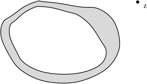
Figure 2: The elementary deformation with the base point $z$.

Let $\delta_{z}$ be variation of any quantity under the elementary deformation with the base point $z$. It is easy to see that $\delta_{z}t_{0}=\epsilon$, $\delta_{z}t_{k}=\epsilon z^{-k}/k$. Indeed,

$$\begin{array}[]{c}\begin{array}[]{l}\displaystyle{\delta_{z}t_{0}=\frac{1}{\pi}\oint\delta n(\xi)|d\xi|=-\frac{\epsilon}{2\pi}\oint\partial_{n}G(z,\xi)|d\xi|=\epsilon}\\ \\ \displaystyle{\delta_{z}t_{k}=\frac{1}{\pi k}\oint\xi^{-k}\delta n(\xi)|d\xi|=-\frac{\epsilon}{2\pi k}\oint\xi^{-k}\partial_{n}G(z,\xi)|d\xi|={\epsilon\over k}z^{-k}}\end{array}\end{array}$$ (2.10)

by virtue of the Dirichlet formula (1.1). Note that the elementary deformation with the base point at $\infty$ keeps all moments except $t_{0}$ fixed. Therefore, the deformation which changes only $t_{0}$ is given by $\delta n(\xi)=-\frac{\epsilon}{2}\partial_{n}G(\infty,\xi)$.

Now we can explicitly define the deformations that change only either $x_{k}=\mbox{Re}\,t_{k}$ or $y_{k}=\mbox{Im}\,t_{k}$ keeping all other moments fixed. As is clear from (2.10), the corresponding $\delta n(\xi)$ is given by the real or imaginary part of normal derivative of the function

$$H_{k}(\xi)=\frac{1}{2\pi i}\oint_{\infty}z^{k}\partial_{z}G(z,\xi)dz$$ (2.11)

at the boundary. Here the contour integral goes around infinity. Namely, the normal displacements $\delta n(\xi)=\epsilon\,{\rm Re}\,(\partial_{n}H_{k}(\xi))$ and $\delta n(\xi)=\epsilon\,{\rm Im}\,(\partial_{n}H_{k}(\xi))$ change the real and imaginary part of $t_{k}$ by $\pm\epsilon$ respectively keeping all other moments fixed.

These deformations allow one to introduce the vector fields

$$\frac{\partial}{\partial t_{0}}\,,\;\;\;\;\frac{\partial}{\partial x_{k}}\,,\;\;\;\;\frac{\partial}{\partial y_{k}}$$

in the space of domains which are locally well-defined. Existence of such vector fields means that the variables $t_{k}$ are independent. For $k>0$ it is more convenient to use their linear combinations

$$\frac{\partial}{\partial t_{k}}=\frac{1}{2}\left(\frac{\partial}{\partial x_{k}}-i\,\frac{\partial}{\partial y_{k}}\right),\;\;\;\;\;\ \frac{\partial}{\partial\bar{t}_{k}}=\frac{1}{2}\left(\frac{\partial}{\partial x_{k}}+i\,\frac{\partial}{\partial y_{k}}\right)$$

which span the complexified tangent space to the space of simply-connected domains (with fixed area $t_{0}$). If $X$ is any functional of our domain locally representable as a function of harmonic moments, $X=X({\bf t})$, the vector fields $\partial_{t_{0}}$, $\partial_{t_{k}}$, $\partial_{\bar{t}_{k}}$ can be understood as partial derivatives acting to the function $X({\bf t})$.

Consider the variation $\delta_{z}X$ of a functional $X=X({\bf t})$ under the elementary deformation with the base point $z$. In the leading order in $\epsilon$ we have:

$$\begin{array}[]{c}\delta_{z}X=\sum_{k}\frac{\partial X}{\partial t_{k}}\,\delta_{z}t_{k}=\epsilon\nabla(z)X\end{array}$$ (2.12)

where the differential operator $\nabla(z)$ is given by

$$\begin{array}[]{c}\nabla(z)=\partial_{t_{0}}+\sum_{k\geq 1}\left(\frac{z^{-k}}{k}\partial_{t_{k}}+\frac{\bar{z}^{-k}}{k}\partial_{\bar{t}_{k}}\right)\end{array}$$ (2.13)

The right hand side suggests that for functionals $X$ such that the series $\nabla(z)X$ converges everywhere in ${\sf D^{c}}$ up to the boundary $\delta_{z}X$ is a harmonic function of the base point $z$.

Note that in [2] we have used the “bump” deformation and continued it harmonically into ${\sf D^{c}}$. In fact, it was the elementary deformation (2.10) $\delta_{z}\propto\oint|d\xi|\partial_{n}G(z,\xi)\delta^{\rm bump}(\xi)$ that was really used. The “bump” deformation should be understood as a (carefully taken) limit of $\delta_{z}$ when the point $z$ tends to the boundary $\partial{\sf D^{c}}$.

The Hadamard formula as integrability condition.

Variation of the Green function under small deformations of the domain is known due to Hadamard, see eq. (1.4). To find how the Green function changes under small variations of the harmonic moments, we fix three points $a,b,c\in{\bf C}\setminus{\sf D}$ and compute $\delta_{c}G(a,b)$ by means of the Hadamard formula (1.4). Using (2.12), one can identify the result with the action of the vector field $\nabla(c)$ on the Green function:

$$\begin{array}[]{c}\nabla(c)G(a,b)=-\,\frac{1}{4\pi}\oint_{\partial{\sf D}}\partial_{n}G(a,\xi)\partial_{n}G(b,\xi)\partial_{n}G(c,\xi)|d\xi|\end{array}$$ (2.14)

Remarkably, the r.h.s. of (2.14) is symmetric in all three arguments, i.e.

$$\begin{array}[]{c}\nabla(a)G(b,c)=\nabla(b)G(c,a)=\nabla(c)G(a,b)\end{array}$$ (2.15)

This is the key relation which allows one to represent the Dirichlet problem as an integrable hierarchy of non-linear differential equations [2], (2.15) being the integrability condition of the hierarchy.

It follows from (2.15) (see [2] for details) that there exists a function $F=F({\bf t})$ such that

$$\begin{array}[]{c}G(z,z^{\prime})=\log\left|{1\over z}-{1\over z^{\prime}}\right|+{1\over 2}\nabla(z)\nabla(z^{\prime})F\end{array}$$ (2.16)

We note that existence of such a representation of the Green function was first conjectured by Takhtajan. For the simply-connected case, this formula was obtained in [14] (see also [13] for a detailed proof and discussion). The function $F$ is (logarithm of) the tau-function of the integrable hierarchy. In [14] it was called the tau-function of the (real analytic) curves – the boundary contours $\partial{\sf D}$ or $\partial{\sf D^{c}}$.

Dispersionless Hirota equations.

Combining (2.16) and (1.2), we obtain the relation

$$\log\left|\frac{w(z)-w(z^{\prime})}{w(z)\overline{w(z^{\prime})}-1}\right|^{2}=\log\left|{1\over z}-{1\over z^{\prime}}\right|^{2}+\nabla(z)\nabla(z^{\prime})F$$ (2.17)

which implies an infinite hierarchy of differential equations on the function $F$. It is convenient to normalize the conformal map $w(z)$ by the conditions that $w(\infty)=\infty$ and $\partial_{z}w(\infty)$ is real, so that

$$w(z)=\frac{z}{r}+O(1)\;\;\;\mbox{as $z\to\infty$}$$ (2.18)

where the real number $r=\lim_{z\to\infty}{dz/dw(z)}$ is called the (external) conformal radius of the domain ${\sf D}$ (equivalently, it can be defined through the Green function as $\log r=\lim_{z\to\infty}(G(z,\infty)+\log|z|)$, see [15]). Then, tending $z^{\prime}\to\infty$ in (2.17), one gets

$$\begin{array}[]{c}\log|w(z)|^{2}=\log|z|^{2}-\partial_{t_{0}}\nabla(z)F\end{array}$$ (2.19)

The limit $z\to\infty$ of this equality yields a simple formula for the conformal radius:

$$\begin{array}[]{c}\log r^{2}=\partial_{t_{0}}^{2}F\end{array}$$ (2.20)

Let us now separate holomorphic and antiholomorphic parts of these equations, introducing the holomorphic and antiholomorphic parts of the operator $\nabla(z)$ (2.13):

$$D(z)=\sum_{k\geq 1}\frac{z^{-k}}{k}\partial_{t_{k}}\,,\;\;\;\;\;\bar{D}(\bar{z})=\sum_{k\geq 1}\frac{\bar{z}^{-k}}{k}\partial_{\bar{t}_{k}}\,,$$ (2.21)

Rewrite (2.17) in the form

$$\begin{array}[]{ll}&\displaystyle{\log\left(\frac{w(z)-w(z^{\prime})}{w(z)\overline{w(z^{\prime})}-1}\right)-\log\left(\frac{1}{z}-\frac{1}{z^{\prime}}\right)-\left(\frac{1}{2}\partial_{t_{0}}+D(z)\right)\nabla(z^{\prime})F}\\ &\\ =&\displaystyle{-\log\left(\frac{\overline{w(z)}-\overline{w(z^{\prime})}}{w(z^{\prime})\overline{w(z)}-1}\right)+\log\left(\frac{1}{\bar{z}}-\frac{1}{\bar{z}^{\prime}}\right)+\left(\frac{1}{2}\partial_{t_{0}}+\bar{D}(\bar{z})\right)\nabla(z^{\prime})F}\end{array}$$

The l.h.s. is a holomorphic function of $z$ while the r.h.s. is antiholomorphic. Therefore, both are equal to a $z$-independent term which can be found from the limit $z\to\infty$. As a result, we obtain the equation

$$\begin{array}[]{c}\log\left(\frac{w(z)-w(z^{\prime})}{w(z)-(\overline{w(z^{\prime})})^{-1}}\right)=\log\left(1-\frac{z^{\prime}}{z}\right)+D(z)\nabla(z^{\prime})F\end{array}$$ (2.22)

which, as $z^{\prime}\to\infty$, turns into the formula for the conformal map $w(z)$:

$$\begin{array}[]{c}\log w(z)=\log z-\frac{1}{2}\partial^{2}_{t_{0}}F-\partial_{t_{0}}D(z)F\end{array}$$ (2.23)

(here we also used (2.20)). Proceeding in a similar way, one can rearrange (2.22) in order to write it separately for holomorphic and antiholomorphic parts in $z^{\prime}$:

$$\begin{array}[]{c}\log\frac{w(z)-w(z^{\prime})}{z-z^{\prime}}\,=\,-\,\frac{1}{2}\partial_{t_{0}}^{2}\,F+D(z)D(z^{\prime})F\end{array}$$ (2.24)

$$\begin{array}[]{c}-\,\log\left(1-\frac{1}{w(z)\overline{w(z^{\prime})}}\right)=D(z)\bar{D}(\bar{z}^{\prime})F\end{array}$$ (2.25)

Writing down eqs. (2.24) for the pairs of points $(a,b)$, $(b,c)$ and $(c,a)$ and summing up the exponentials of the both sides of each equation one arrives at the relation

$$\begin{array}[]{c}(a-b)e^{D(a)D(b)F}+(b-c)e^{D(b)D(c)F}+(c-a)e^{D(c)D(a)F}=0\end{array}$$ (2.26)

which is the dispersionless Hirota equation (for the KP part of the two-dimensional Toda lattice hierarchy) written in the symmetric form. This equation can be regarded as a very degenerate case of the trisecant Fay identity [9]. It encodes the algebraic relations between the second order derivatives of the function $F$. As $c\to\infty$, we get these relations in a more explicit but less symmetric form:

$$\begin{array}[]{c}1-e^{D(a)D(b)F}=\frac{D(a)-D(b)}{a-b}\,\partial_{t_{1}}F\end{array}$$ (2.27)

which makes it clear that the totality of second derivatives $F_{ij}:=\partial_{t_{i}}\partial_{t_{j}}F$ are expressed through the derivatives with one of the indices put equal to unity.

More general equations of the dispersionless Toda hierarchy obtained in a similar way by combining eqs. (2.23), (2.24) and (2.25) include derivatives w.r.t. $t_{0}$ and $\bar{t}_{k}$:

$$\begin{array}[]{c}(a-b)e^{D(a)D(b)F}=ae^{-\partial_{t_{0}}D(a)F}-be^{-\partial_{t_{0}}D(b)F}\end{array}$$ (2.28)

$$\begin{array}[]{c}1-e^{-D(z)\bar{D}(\bar{z})F}=\frac{1}{z\bar{z}}e^{\partial_{t_{0}}\nabla(z)F}\end{array}$$ (2.29)

These equations allow one to express the second derivatives $\partial_{t_{m}}\partial_{t_{n}}F$, $\partial_{t_{m}}\partial_{\bar{t}_{n}}F$ with $m,n\geq 1$ through the derivatives $\partial_{t_{0}}\partial_{t_{k}}F$, $\partial_{t_{0}}\partial_{\bar{t}_{k}}F$. In particular, the dispersionless Toda equation,

$$\begin{array}[]{c}\partial_{t_{1}}\partial_{\bar{t}_{1}}F=e^{\partial_{t_{0}}^{2}F}\end{array}$$ (2.30)

which follows from (2.29) as $z\to\infty$, expresses $\partial_{t_{1}}\partial_{\bar{t}_{1}}F$ through $\partial_{t_{0}}^{2}F$.

For a comprehensive exposition of Hirota equations for dispersionless KP and Toda hierarchies we refer the reader to [16, 17].

Integral representation of the tau-function.

Eq. (2.16) allows one to obtain a representation of the tau-function as a double integral over the domain ${\sf D}$. Set $\tilde{\Phi}(z):=\nabla(z)F$. One is able to determine this function via its variation under the elementary deformation:

$$\delta_{a}\tilde{\Phi}(z)=-2\epsilon\log\left|a^{-1}-z^{-1}\right|+2\epsilon G(a,z)$$ (2.31)

which is read from eq. (2.16) by virtue of (2.12). This allows one to identify $\tilde{\Phi}$ with the “modified potential” $\tilde{\Phi}(z)=\Phi(z)-\Phi(0)+t_{0}\log|z|^{2}$, where $\Phi$ is given by (2.4). Thus we can write

$$\begin{array}[]{c}\nabla(z)F=\tilde{\Phi}(z)=-\frac{2}{\pi}\int_{{\sf D}}\log|z^{-1}-\zeta^{-1}|d^{2}\zeta=v_{0}+2{\rm Re}\sum_{k>0}\frac{v_{k}}{k}z^{-k}\end{array}$$ (2.32)

The last equality is to be understood as the Taylor expansion around infinity. The coefficients $v_{k}$ are moments of the interior domain (the “dual” harmonic moments) defined as

$$\begin{array}[]{c}v_{k}=\frac{1}{\pi}\int_{{\sf D}}z^{k}\,d^{2}z\ \ \ (k>0)\,,\;\;\;\;\;v_{0}=-\Phi(0)=\frac{2}{\pi}\int_{{\sf D}}\log|z|d^{2}z\end{array}$$ (2.33)

From (2.32) it is clear that

$$\begin{array}[]{c}v_{k}=\partial_{t_{k}}F\,,\;\;\;\;k\geq 0\end{array}$$ (2.34)

i.e., the moments of the complementary domain ${\sf D}$ (the “dual” moments) are completely determined by the function $F$ of harmonic moments of ${\sf D^{c}}$.

In a similar manner, one arrives at the integral representation of the tau-function. Comparing (2.32) with (2.31) one can easily notice that the meaning of the elementary deformation $\delta_{\xi}$ or the operator $\nabla(\xi)$ formally applied at the boundary point $\xi\in\partial{\sf D}$ (where $G(z,\xi)=0$) is attaching a “small piece” to the integral over the domain ${\sf D}$ (the “bump” operator from [2]). Using this fact and interpreting (2.32) as a variation $\delta_{z}F$ we arrive at the double-integral representation of the tau-function

$$\begin{array}[]{c}F=-\frac{1}{\pi^{2}}\int_{{\sf D}}\!\int_{{\sf D}}\log|z^{-1}-\zeta^{-1}|d^{2}zd^{2}\zeta\end{array}$$ (2.35)

or

$$\begin{array}[]{c}F=\frac{1}{2\pi}\int_{{\sf D}}\tilde{\Phi}(z)d^{2}z=\frac{1}{2\pi}\int_{\sf D}\left(\Phi(z)-2\Phi(0)\right)d^{2}z\end{array}$$ (2.36)

As we see below, the main formulas from this paragraph remain intact in the multiply-connected case.

3 The Dirichlet problem and the tau-function in the multiply-connected case

Let now ${\sf D}_{\alpha}$, $\alpha=0,1,\ldots,g$, be a collection of $g+1$ non-intersecting bounded connected domains in the complex plane with smooth boundaries $\partial{\sf D}_{\alpha}$. Set ${\sf D}=\cup_{\alpha=0}^{g}{\sf D}_{\alpha}$, so that the complement ${\sf D^{c}}={\bf C}\setminus{\sf D}$ becomes a multiply-connected unbounded domain in the complex plane (see fig. 3). Let ${\sf b}_{\alpha}$ be the boundary curves. They are assumed to be positively oriented as boundaries of ${\sf D^{c}}$, so that $\cup_{\alpha=0}^{g}{\sf b}_{\alpha}=\partial{\sf D^{c}}$ while ${\sf b}_{\alpha}=-\partial{\sf D}_{\alpha}$ has the clockwise orientation.

Figure 3: A multiply-connected domain ${\sf D^{c}}={\bf C}\setminus{\sf D}$ for $g=3$. The domain ${\sf D}=\bigcup_{\alpha=0}^{3}{\sf D}_{\alpha}$ consists of $g+1=4$ disconnected parts ${\sf D}_{\alpha}$ with the boundaries ${\sf b}_{\alpha}$. To define the complete set of harmonic moments, we also need the auxiliary points $z_{\alpha}\in{\sf D}_{\alpha}$ which should be always located inside the corresponding domains.

Comparing to the simply-connected case, nothing is changed in posing the standard Dirichlet problem. The definition of the Green function and the formula (1.1) for the solution of the Dirichlet problem through the Green function remain to be the same.

A difference is in the nature of harmonic functions. Any harmonic function is still the real part of an analytic function but in the multiply-connected case these analytic funstions are not necessarily single-valued (only their real parts have to be single-valued). In other words, the harmonic functions may have non-zero “periods” over non-trivial cycles. In our case, the non-trivial cycles are the boundary curves ${\sf b}_{\alpha}$. In general, the Green function has non-zero “periods” over all boundary contours. Hence it is natural to introduce new objects, specific to the multiply-connected case, which are defined as “periods” of the Green function.

First, the harmonic measure $\omega_{\alpha}(z)$ of the boundary component ${\sf b}_{\alpha}$ is the harmonic function in ${\sf D^{c}}$ such that it is equal to unity on ${\sf b}_{\alpha}$ and vanishes on the other boundary curves. Thus the harmonic measure is the solution to the particular Dirichlet problem. From the general formula (1.1) we conclude that

$$\begin{array}[]{c}\omega_{\alpha}(z)=-\,\frac{1}{2\pi}\oint_{{\sf b}_{\alpha}}\partial_{n}G(z,\zeta)|d\zeta|,\ \ \ \ \ \ \alpha=1,\ldots,g\end{array}$$ (3.1)

so the harmonic measure is the period of the Green function w.r.t. one of its arguments. From the maximum principle for harmonic functions it follows that $0<\omega_{\alpha}(z)<1$ in internal points. Obviously, $\sum_{\alpha=0}^{g}\omega_{\alpha}(z)=1$. In what follows we consider the linear independent functions $\omega_{\alpha}(z)$ with $\alpha=1,\ldots,g$.

Further, taking “periods” in the remaining variable, we define

$$\Omega_{\alpha\beta}=-\frac{1}{2\pi}\oint_{{\sf b}_{\beta}}\partial_{n}\omega_{\alpha}(\zeta)|d\zeta|,\ \ \ \ \ \ \alpha,\beta=1,\ldots,g$$ (3.2)

The matrix $\Omega_{\alpha\beta}$ is known to be symmetric, non-degenerate and positively-definite. It will be clear below that the matrix $T_{\alpha\beta}=i\pi\Omega_{\alpha\beta}$ can be identified with the matrix of periods of holomorphic differentials on the Schottky double of the domain ${\sf D^{c}}$ (see formula (3.5)). For brevity, we refer to both $T_{\alpha\beta}$ and $\Omega_{\alpha\beta}$ as period matrices.

For the harmonic measure and the period matrix there are variational formulas similar to the Hadamard formula (1.4). They can be derived either by a direct variation of (3.1) and (3.2) using the Hadamard formula or (much easier) by a “pictorial” argument like in fig. 1. The formulas are:

$$\delta\omega_{\alpha}(z)=\frac{1}{2\pi}\oint_{\partial{\sf D}}\partial_{n}G(z,\xi)\,\partial_{n}\omega_{\alpha}(\xi)\,\delta n(\xi)\,|d\xi|$$ (3.3)

$$\delta\Omega_{\alpha\beta}=\frac{1}{2\pi}\oint_{\partial{\sf D}}\partial_{n}\omega_{\alpha}(\xi)\,\partial_{n}\omega_{\beta}(\xi)\,\delta n(\xi)\,|d\xi|$$ (3.4)

The Schottky double.

It is customary to associate with a planar multiply-connected domain its Schottky double (see, e.g., [18], Ch. 2.2), a compact Riemann surface without boundary endowed with antiholomorpic involution, the boundary of the initial domain being the set of the fixed points of the involution. The Schottky double of the multiply-connected domain ${\sf D^{c}}$ can be thought of as two copies of ${\sf D^{c}}$ (“upper” and “lower” sheets of the double) glued along the boundaries $\cup_{\alpha=0}^{g}{\sf b}_{\alpha}=\partial{\sf D^{c}}$, with points at infinity added ($\infty$ and $\bar{\infty}$). In this set-up the holomorphic coordinate on the upper sheet is $z$ inherited from ${\sf D^{c}}$, while the holomorphic coordinate on the other sheet is $\bar{z}$. The Schottky double of ${\sf D^{c}}$ with two infinities added is a compact Riemann surface $\Sigma$ of genus $g=\#\{{\sf D}_{\alpha}\}-1$. A meromorphic function on the double is a pair of meromorphic functions $f,\tilde{f}$ on ${\sf D^{c}}$ such that $f(z)=\tilde{f}(\bar{z})$ on the boundary. Similarly, a meromorphic differential on the double is a pair of meromorphic differentials $f(z)dz$ and $\tilde{f}(\bar{z})d\bar{z}$ such that $f(z)dz=\tilde{f}(\bar{z})d\bar{z}$ along the boundary curves.

Figure 4: The domain ${\sf D^{c}}$ with the ${\sf a}_{\alpha}$-cycle, going one way along the “upper sheet” and back along the “lower sheet” of the Schottky double of ${\sf D^{c}}$. For such choice one clearly gets the intersection form ${\sf a}_{\alpha}\circ{\sf b}_{\beta}=\delta_{\alpha\beta}$ for $\alpha,\beta=1,\dots,g$.

On the double, one may choose a canonical basis of cycles. We fix the ${\sf b}$-cycles to be just the boundaries of the holes ${\sf b}_{\alpha}$ for $\alpha=1,\ldots,g$. Note that regarded as the oriented boundaries of ${\sf D^{c}}$ (not ${\sf D}$) they have the clockwise orientation. The ${\sf a}_{\alpha}$-cycle connects the $\alpha$-th hole with the 0-th one. To be more precise, fix points $\xi_{\alpha}$ on the boundaries, then the ${\sf a}_{\alpha}$ cycle starts from $\xi_{0}$, goes to $\xi_{\alpha}$ on the “upper” (holomorphic) sheet of the double and goes back the same way on the “lower” sheet, where the holomorphic coordinate is $\bar{z}$, see fig. 4.

Being harmonic, $\omega_{\alpha}$ can be represented as the real part of a holomorphic function:

$$\omega_{\alpha}(z)=W_{\alpha}(z)+\overline{W_{\alpha}(z)}$$

where $W_{\alpha}(z)$ are holomorphic multivalued functions in ${\sf D^{c}}$. The differentials $dW_{\alpha}$ are holomorphic in ${\sf D^{c}}$ and purely imaginary on all boundary contours. So they can be extended holomorphically to the lower sheet as $-d\overline{W_{\alpha}(z)}$. In fact this is the canonically normalized basis of holomorphic differentials on the double: according to the definitions,

$$\oint_{{\sf a}_{\alpha}}\!dW_{\beta}=\int_{\xi_{0}}^{\xi_{\alpha}}dW_{\beta}(z)+\int_{\xi_{\alpha}}^{\xi_{0}}\left(-d\overline{W_{\beta}(z)}\right)=2{\rm Re}\int_{\xi_{0}}^{\xi_{\alpha}}dW_{\beta}(z)=\omega_{\beta}(\xi_{\alpha})\!-\!\omega_{\beta}(\xi_{0})=\delta_{\alpha\beta}$$

Then the matrix of ${\sf b}$-periods of these differentials reads

$$\begin{array}[]{c}T_{\alpha\beta}=\oint_{{\sf b}_{\alpha}}dW_{\beta}=-\frac{i}{2}\oint_{{\sf b}_{\alpha}}\partial_{n}\omega_{\beta}dl=i\pi\Omega_{\alpha\beta}\end{array}$$ (3.5)

i.e. the period matrix $T_{\alpha\beta}$ of the Schottky double $\Sigma$ is a purely imaginary non-degenerate matrix with positively definite imaginary part $\pi\Omega_{\alpha\beta}$ (3.2).

Harmonic moments of multiply-connected domains.

One may still use harmonic moments to characterize the shape of a multiply-connected domain. However, the set of harmonic functions should be extended by adding functions with poles in any hole (not only in ${\sf D}_{0}$ as before) and functions whose holomorphic parts are not single-valued. To specify them, let us mark points $z_{\alpha}\in{\sf D}_{\alpha}$, one in each hole (see fig. 3). Without loss of generality, it is convenient to put $z_{0}=0$. Then one may consider single-valued analytic functions in ${\sf D^{c}}$ of the form $(z-z_{\alpha})^{-k}$ and harmonic functions $\log\left|1-{z_{\alpha}\over z}\right|^{2}$ with multi-valued analytic part.

The arguments almost identical to the ones used in the simply-connected case show that the parameters $t_{0},M_{n,\alpha},\phi_{\alpha}$, where as in (2.3) $t_{0}=\mbox{Area}({\sf D})/\pi$,

$$\begin{array}[]{c}M_{n,\,\alpha}=-{1\over\pi}\int_{{\sf D^{c}}}(z-z_{\alpha})^{-n}d^{2}z,\;\;\;\;\;\alpha=0,1,\ldots,g,\;\;n\geq 1\end{array}$$ (3.6)

together with their complex conjugate, and

$$\begin{array}[]{c}\phi_{\alpha}=-{1\over\pi}\int_{{\sf D^{c}}}\log\left|1-\frac{z_{\alpha}}{z}\right|^{2}d^{2}z,\;\;\;\;\;\alpha=1,\ldots,g\end{array}$$ (3.7)

uniquely define ${\sf D^{c}}$, i.e. any deformation preserving these parameters is trivial. Note that the extra moments $\phi_{\alpha}$ are essentially the values of the potential (2.4) at the points $z_{\alpha}$

$$\begin{array}[]{c}\phi_{\alpha}=\Phi(0)-\Phi(z_{\alpha})-|z_{\alpha}|^{2}\end{array}$$ (3.8)

A crucial step for what follows is the change of variables from $M_{n,\alpha}$ to the variables $\tau_{k}$ which are finite linear combinations of the $M_{n,\alpha}$’s. They can be directly defined as moments with respect to new basis of functions:

$$\begin{array}[]{c}\tau_{0}=t_{0},\ \ \ {\tau}_{k}={1\over 2\pi i}\oint_{\partial{\sf D}}A_{k}(z)\bar{z}dz=-{1\over\pi}\int_{{\sf D}^{c}}d^{2}zA_{k}(z),\ \ \ k>0\end{array}$$ (3.9)

The functions $A_{k}(z)$ are analogous to the Laurent-Fourier type basis on Riemann surfaces introduced in [8]. They are explicitly defined by the following formulas (here the indices $\alpha$ and $\beta$ are understood modulo $g+1$):

$$\begin{array}[]{c}A_{m(g+1)+\alpha}=R^{-m}(z)\prod_{\beta=0}^{\alpha-1}(z-z_{\beta})^{-1}\\ R(z)=\prod_{\beta=0}^{g}(z-z_{\beta})\end{array}$$ (3.10)

In a neighbourhood of infinity $A_{k}(z)=z^{-k}+O(z^{-k-1})$. Any analytic function in ${\sf D^{c}}$ vanishing at infinity can be represented as a linear combination of $A_{k}$ which is convergent in domains such that $|R(z)|>{\rm const}$. In the case of one hole ($g=0$) the formulas (3.10) give the basis used in the previous section: $A_{k}=z^{-k}$. Note that $A_{0}=1$, $A_{1}=1/z$, therefore $\tau_{0}=t_{0}$ and $\tau_{1}=M_{1,0}=t_{1}$.

Local coordinates in the space of multiply-connected domains.

Now we are going to prove that the parameters $\tau_{k}$, $\phi_{\alpha}$ can be treated as local coordinates in the space of multiply-connected domains. (Here we use the same restricted notion of the local coordinates, as in the simply connected case (see Remark in the Section 2)).

It is instructive and simpler first to prove this for another choice of parameters. Instead of $\phi_{\alpha}$ one may use the areas of the holes

$$\begin{array}[]{c}s_{\alpha}=\frac{\mbox{Area}({\sf D}_{\alpha})}{\pi}=\frac{1}{\pi}\int_{{\sf D}_{\alpha}}d^{2}z=\frac{1}{2\pi i}\oint_{\partial{\sf D}_{\alpha}}\bar{z}dz\,,\;\;\;\;\;\alpha=1,\ldots,g\end{array}$$ (3.11)

In order to prove that any deformation that preserves $\tau_{k}$ and $s_{\alpha}$ is trivial, we introduce the basis of differentials $dB_{k}$ which satisfy the defining “orthonormality” relations

$$\begin{array}[]{c}\frac{1}{2\pi i}\oint_{\partial{\sf D}}A_{k}dB_{k^{\prime}}=\delta_{k,k^{\prime}}\end{array}$$ (3.12)

for all integer $k,k^{\prime}$. It is easy to see that explicitly they are given by:

$$\begin{array}[]{c}dB_{m(g+1)+\alpha}={dzR^{m}(z)\over z-z_{g}}\prod_{\beta=0}^{\alpha-1}(z-z_{\beta-1})\end{array}$$ (3.13)

where we identify $z_{-1}\equiv z_{g}$. The existence of a well-defined “dual” basis of differentials obeying the orthonormality relation is the key feature of the basis functions $A_{k}$, which makes $\tau_{k}$ good local coordinates comparing to the $M_{n,\alpha}$. For the functions $(z-z_{\alpha})^{-n}$ one cannot define the dual basis.

The summation formulas

$$\begin{array}[]{c}{dzd\zeta\over\zeta-z}=\sum_{n=1}^{\infty}d\zeta A_{n}(\zeta)dB_{n}(z),\ \ \ |R(z)|<|R(\zeta)|\\ {dzd\zeta\over\zeta-z}=-\sum_{n=0}^{\infty}d\zeta A_{-n}(\zeta)dB_{-n}(z),\ \ \ |R(z)|>|R(\zeta)|\end{array}$$ (3.14)

which can be checked directly, allow us to repeat arguments of sect. 2. Indeed, the Cauchy integral (2.6),

$$C(z)dz={dz\over 2\pi i}\oint_{\partial{\sf D}}{\bar{\zeta}d\zeta\over\zeta-z}$$ (3.15)

where the integration now goes along all boundary components, defines in each of the holes ${\sf D_{\alpha}}$ analytic differentials $C^{\alpha}(z)dz$ (analogs of $C^{+}(z)dz$ in the simply-connected case). In the complementary domain ${\sf D^{c}}$ the Cauchy integral still defines the differential $C^{-}(z)dz$ holomorphic everywhere in ${\sf D^{c}}$ except for infinity where it has a simple pole. The difference of the boundary values of the Cauchy integral is equal to $\bar{z}$:

$$C^{\alpha}(z)-C^{-}(z)=\bar{z}\,,\;\;\;\;\;\;z\in\partial{\sf D}_{\alpha}$$

From equation (2.7), which can be written separately for each contour, it follows that

• The difference of the boundary values

  $$\left(\partial_{t}C^{\alpha}(\zeta)-\partial_{t}C^{-}(\zeta)\right)d\zeta$$

  of the derivative of the Cauchy integral (3.15) is, for all $\alpha$, a purely imaginary differential on the boundary ${\sf b}_{\alpha}$.

The expansion (3.14) of the Cauchy kernel implies that

• If a $t$-deformation preserves all the moments $\tau_{k}$, $k\geq 0$, then $\partial_{t}\bar{\zeta}d\zeta-\partial_{t}\zeta d\bar{\zeta}$ extends to a holomorphic differential in ${\sf D^{c}}$.

Indeed, since $|R(z)|$ is small for $z$ close enough to any of the points $z_{\alpha}$, one can expand $\partial_{t}C^{\alpha}(z)$ for any $\alpha$ as

$$\begin{array}[]{c}\partial_{t}C^{\alpha}(z)dz={1\over 2\pi i}\sum_{k=1}^{\infty}dB_{k}\partial_{t}\left(\oint_{\partial{\sf D}}A_{k}(\zeta)\bar{\zeta}d\zeta\right)=\sum_{k=1}^{\infty}\partial_{t}\tau_{k}\ dB_{k}(z)\end{array}$$ (3.16)

and conclude that it is identically zero provided $\partial_{t}\tau_{k}=0$. Hence $-\partial_{t}C^{-}(z)dz$ is the desired extension of $\partial_{t}\bar{\zeta}d\zeta-\partial_{t}\zeta d\bar{\zeta}$. It has no pole at infinity due to the equation $\partial_{t}\tau_{0}=0$.

Using the Schwarz symmetry principle we obtain that $\partial_{t}C^{-}(z)dz$ extends to a holomorphic differential on the Schottky double. If the variables $s_{\alpha}$ are also preserved under the $t$-deformation, then this holomorphic differential has zero periods along all the cycles ${\sf b}_{\alpha}$. Therefore, it is identically zero. This completes the proof of the statement that any deformation of the domain preserving $\tau_{k}$ and $s_{\alpha}$ is trivial.

In this proof the variables $s_{\alpha}$ were used only at the last moment in order to show that the extension of $\partial_{t}C^{-}(z)dz$ as a holomorphic differential on the Schottky double is trivial. The variables $\phi_{\alpha}$ can be used in a similar way. Namely, let us show that if they are preserved under $t$-deformation then ${\sf a}_{\alpha}$-periods of the extension of $\partial_{t}C^{-}(z)dz$ are trivial, and therefore this extension is identically zero. Indeed, the variable $\phi_{\alpha}$ (3.7) can be represented in the form

$$\begin{array}[]{c}\phi_{\alpha}=-{2\over\pi}{\rm Re}\int_{0}^{z_{\alpha}}dz\int_{{\sf D^{c}}}\frac{d^{2}\zeta}{z-\zeta}\end{array}$$ (3.17)

The differential $\frac{dz}{\pi}\int_{{\sf D^{c}}}\frac{d^{2}\zeta}{z-\zeta}$ is equal to $C^{\alpha}(z)dz$ for $z\in{\sf D}_{\alpha}$ and $(\bar{z}+C^{-}(z))dz$ for $z\in{\sf D^{c}}$. Let $\xi_{0}$, $\xi_{\alpha}$ be the points where the integration path from $0$ to $z_{\alpha}$ intersects the boundary contours ${\sf b}_{0}$, ${\sf b}_{\alpha}$. Then

$$\begin{array}[]{c}\phi_{\alpha}=-2\,{\rm Re}\left(\int_{0}^{\xi_{0}}C^{0}(z)dz+\int_{\xi_{\alpha}}^{z_{\alpha}}C^{\alpha}(z)dz+\int_{\xi_{0}}^{\xi_{\alpha}}(\bar{z}+C^{-}(z))dz\right)\end{array}$$ (3.18)

It is shown above that if a $t$-deformation preserves the variables $\tau_{k}$ then all $\partial_{t}C^{\alpha}(z)dz=0$. Thus vanishing of the $t$-derivative $\partial_{t}\phi_{\alpha}=0$ implies

$$\begin{array}[]{c}0=-\partial_{t}\phi_{\alpha}=2\,{\rm Re}\int_{\xi_{0}}^{\xi_{\alpha}}\partial_{t}C^{-}(z)dz\end{array}$$ (3.19)

The r.h.s of this equation is just the ${\sf a}_{\alpha}$-period of the holomorphic extension of the differential $\partial_{t}C^{-}(z)dz$.

Let us construct the deformations $\partial_{x_{k}}^{\phi}$ and $\partial_{y_{k}}^{\phi}$ of the boundary that change the real or imaginary parts of the variable $\tau_{k}=x_{k}+iy_{k}$, $k\geq 1$, keeping all the other moments and the variables $\phi_{\alpha}$ fixed. It is convenient to set $\partial_{\tau_{k}}^{\phi}=\frac{1}{2}(\partial_{x_{k}}^{\phi}-i\partial_{y_{k}}^{\phi})$. The argument is similar to the proof of the fact that any deformation that preserves all the variables is trivial.

• Suppose that the deformations $\partial_{x_{k}}^{\phi}$ and $\partial_{y_{k}}^{\phi}$ exist. Then the differential $\partial_{\tau_{k}}^{\phi}\bar{\zeta}d\zeta-\partial_{\tau_{k}}^{\phi}\zeta d\bar{\zeta}$ extends from $\partial{\sf D^{c}}$ to the Schottky double $\Sigma$. Its extension is a meromorphic differential $d\Omega_{k}^{\phi}$ with the only pole at the infinity point $\infty$ on the upper sheet. In a neighborhood of $\infty$ it has the form

  $$\begin{array}[]{c}d\Omega_{k}^{\phi}(z)=dB_{k}(z)+O(z^{-2})dz\end{array}$$ (3.20)

  The ${\sf a}$-periods of $d\Omega_{k}^{\phi}$ are equal to

  $$\oint_{{\sf a}_{\alpha}}d\Omega_{k}^{\phi}=\int_{0}^{z_{\alpha}}dB_{k}$$ (3.21)

First of all, it is clear that the meromorphic differential $d\Omega_{k}^{\phi}$ on $\Sigma$ is uniquely defined by its asymptotics at $\infty$ and by the normalization (3.21) of its ${\sf a}$-periods. To deduce these properties, we notice, using (3.16), that $\partial_{x_{k}}C^{\alpha}(z)dz=dB_{k}(z)$. Therefore, the differential $\partial_{x_{k}}^{\phi}\bar{\zeta}d\zeta-\partial_{x_{k}}^{\phi}\zeta d\bar{\zeta}$ extends to ${\sf D^{c}}$ as

$$\begin{array}[]{c}d\Omega_{x_{k}}^{\phi}=-\partial_{x_{k}}C^{-}(z)dz+dB_{k}\end{array}$$ (3.22)

Using the Schwarz symmetry principle we conclude that it extends to the Schottky double as a meromorphic differential. Around the two infinities it has the form $d\Omega_{x_{k}}^{\phi}\ \mathrel{\mathop{=}\limits_{z\to\infty}}\ dB_{k}+O(z^{-2})dz$ and $d\Omega_{x_{k}}^{\phi}\ \mathrel{\mathop{=}\limits_{\bar{z}\to\bar{\infty}}}\ -d\bar{B}_{k}+O(\bar{z}^{-2})d\bar{z}$. In the same way one gets that the differential $\partial_{y_{n}}^{\phi}\bar{\zeta}d\zeta-\partial_{y_{n}}^{\phi}\zeta d\bar{\zeta}$ extends to the double as a meromorphic differential $d\Omega_{y_{k}}^{\phi}$, which at the two infinities has the form $d\Omega_{y_{k}}^{\phi}\ \mathrel{\mathop{=}\limits_{z\to\infty}}\ idB_{k}+O(z^{-2})dz$ and $d\Omega_{y_{k}}^{\phi}\ \mathrel{\mathop{=}\limits_{\bar{z}\to\bar{\infty}}}\ id\bar{B}_{k}+O(\bar{z}^{-2})d\bar{z}$ respectively. Since

$$2d\Omega_{k}^{\phi}=d\Omega_{x_{k}}^{\phi}-id\Omega_{y_{k}}^{\phi}$$

the first statement is proven. From $\partial_{x_{k}}^{\phi}\phi_{\alpha}=0$ and (3.17), (3.22) it follows that

$$0={\rm Re}\left(\int_{0}^{\xi_{0}}dB_{k}+\int_{\xi_{0}}^{\xi_{\alpha}}\left(-d\Omega_{x_{k}}^{\phi}+dB_{k}\right)+\int_{\xi_{\alpha}}^{z_{\alpha}}dB_{k}\right)$$

Hence

$$\oint_{{\sf a}_{\alpha}}d\Omega_{x_{k}}^{\phi}=2{\rm Re}\int_{0}^{z_{\alpha}}dB_{k}$$

In the same way one gets

$$\oint_{{\sf a}_{\alpha}}d\Omega_{y_{k}}^{\phi}=-2{\rm Im}\int_{0}^{z_{\alpha}}\,dB_{k}$$

The last two equations are equivalent to (3.21).

Normal displacement of the boundary that accomplishes the deformations can be explicitly found using the following elementary proposition.

• Let ${\sf D}(t)$ be a deformation with real parameter $t$ such that the differential

  $$d\Omega=\partial_{t}\bar{\zeta}d\zeta-\partial_{t}\zeta d\bar{\zeta}$$

  extends to a meromorphic differential $d\Omega$ globally defined on the Schottky double $\Sigma$. Then the corresponding normal displacement of the boundary is proportional to normal derivative of ${\rm Re}\int^{z}d\Omega$ at the boundary point $\xi$:

  $$\delta n(\xi)=\frac{1}{2}\delta t\,\partial_{n}\left({\rm Re}\int^{\xi}d\Omega\right)$$ (3.23)

  Conversely, if $\delta n(\xi)=\frac{1}{2}\delta t\,\partial_{n}H(\xi)$, where $H$ is a real-valued function such that $dH=0$ along the boundary contours and $\partial_{z}H$ is meromorphic in ${\sf D^{c}}$ then the differential $\partial_{t}\bar{\zeta}d\zeta-\partial_{t}\zeta d\bar{\zeta}$ is meromorphically extendable to the Schottky double as $2\partial_{z}Hdz$ on the upper sheet and $-2\partial_{\bar{z}}Hd\bar{z}$ on the lower sheet.

In our case normal displacements of the boundary that change $x_{k}$ or $y_{k}$ keeping all the other moments and the variables $\phi_{\alpha}$ fixed are thus given by

$$\delta n(\xi)=\frac{1}{2}\delta x_{k}\,\partial_{n}\left({\rm Re}\int^{\xi}d\Omega_{x_{k}}^{\phi}\right),\;\;\;\;\delta n(\xi)=\frac{1}{2}\delta y_{k}\,\partial_{n}\left({\rm Re}\int^{\xi}d\Omega_{y_{k}}^{\phi}\right)$$ (3.24)

respectively. Note that since the differentials $d\Omega_{x_{k}}(z)$, $d\Omega_{y_{k}}(z)$ (but not $d\Omega_{k}(z)$!) are purely imaginary on the boundaries, $d\,{\rm Re}\,\Omega_{x_{k}}(z)=d\,{\rm Re}\,\Omega_{y_{k}}(z)=0$ along each component of the boundary. With formulas (3.24) at hand, one can directly verify that these deformations indeed change $x_{k}$ or $y_{k}$ only and keep fixed all other moments. We leave this to the reader.

In terms of the differential $d\Omega_{k}^{\phi}$ formulas (3.24) acquire the form

$$\delta n(\xi)=\delta x_{k}\,\partial_{n}\left({\rm Re}\int^{\xi}d\Omega_{k}^{\phi}\right),\;\;\;\;\delta n(\xi)=-\delta y_{k}\,\partial_{n}\left({\rm Im}\int^{\xi}d\Omega_{k}^{\phi}\right)$$ (3.25)

(cf. (2.11) for the simply-connected case). Indeed, taking the real part of $2\Omega_{k}(\xi)=\Omega_{x_{k}}(\xi)-i\Omega_{y_{k}}(\xi)$, we get $2\,{\rm Re}\,\Omega_{k}(\xi)=\,{\rm Re}\,\Omega_{x_{k}}(\xi)+\,{\rm Im}\,\Omega_{y_{k}}(\xi)$. But the normal derivative of ${\rm Im}\,\Omega_{y_{k}}(\xi)$ vanishes since, by virtue of the Cauchy-Riemann identities, it is equal to the tangential derivative of the conjugate harmonic function ${\rm Re}\,\Omega_{y_{k}}(\xi)$. This proves the first formula in (3.25). The second one is proven in a similar way by taking imaginary part of $2\Omega_{k}(\xi)$.

The construction of the vector fields $\partial_{\tau_{0}}^{\phi}$ (which changes $\tau_{0}$ only) and $\partial_{\alpha}^{\phi}$ (which changes $\phi_{\alpha}$ only) is quite similar and even simpler since the derivative (3.16) vanishes. So, we present the results without going into details.

• The deformation $\partial_{\tau_{0}}^{\phi}$ corresponds to the normal displacement

  $$\delta n(\xi)=-\frac{1}{2}\delta\tau_{0}\,\partial_{n}G(\infty,\xi)$$

  The differential $-(\partial_{\tau_{0}}^{\phi}\bar{\zeta}d\zeta-\partial_{\tau_{0}}^{\phi}\zeta d\bar{\zeta})$ extends from $\partial{\sf D^{c}}$ to the Schottky double $\Sigma$. Its extension is a meromorphic third-kind Abelian differential $d\Omega_{0}$ which has simple poles at the infinities on the two sheets of the Schottky double (with residues $\pm 1$) and vanishing ${\sf a}$-periods.

• The deformation $\partial_{\alpha}^{\phi}$ corresponds to the normal displacement

  $$\delta n(\xi)=\frac{1}{4}\delta\phi_{\alpha}\,\partial_{n}\omega_{\alpha}(\xi)$$

  where $\omega_{\alpha}$ is the harmonic measure of the boundary component ${\sf b}_{\alpha}$ (see (3.1)). The differential $\partial_{\alpha}^{\phi}\bar{\zeta}d\zeta-\partial_{\alpha}^{\phi}\zeta d\bar{\zeta}$ holomorphically extends from $\partial{\sf D^{c}}$ to the Schottky double $\Sigma$. Its extension is the canonically normalized holomorphic differential $dW_{\alpha}=\partial_{z}\omega_{\alpha}(z)dz$ on the upper sheet (and $dW_{\alpha}=-\partial_{\bar{z}}\omega_{\alpha}(z)d\bar{z}$ on the lower sheet).

So we see that $\partial_{x_{k}}^{\phi}$, $\partial_{y_{k}}^{\phi}$, $\partial_{\tau_{0}}^{\phi}$ and $\partial_{\alpha}^{\phi}$ are well-defined vector fields on the space of multiply-connected domains. This fact allows us to treat $\phi_{\alpha}$, $\tau_{k}$ as local coordinates on this space. At this stage it becomes clear why we prefer to use the moments $\tau_{k}$ rather than $M_{k,\alpha}$. Although the latter are finite linear combinations of the former, they can not be treated as local coordinates because the vector fields $\partial/\partial M_{k,\alpha}$, being in general infinite linear combinations of the $\partial_{\tau_{k}}^{\phi}$, are not well-defined.

$\Pi$-variables.

Up to now the roles of the variables $s_{\alpha}$ and $\phi_{\alpha}$ have been in some sense dual to each other. It is necessary to emphasize that this duality does not go beyond the framework of our proof of the statement that the first or the second sets together with the variables $\tau_{k}$ are local coordinates in the space of multiply-connected domains. For analytic boundary curves one can define the Schwarz function, which is a unique function analytic in some strip-like neighborhoods of all boundaries such that

$$S(z)=\bar{z}\;\;\;\;\;\mbox{on the boundary curves}$$ (3.26)

Then the variables $s_{\alpha}$ are ${\sf b}$-periods of the differential $S(z)dz$. At the same time, the variables $\phi_{\alpha}$ in general can not be identified with periods of this differential (or its extension) over any cycles on the Schottky double. Now we are going to introduce new variables, $\Pi_{\alpha}$, which can be called virtual ${\sf a}$-periods of the differential $S(z)dz$ on the Schottky double, since in all the cases when the Schwarz function has a meromorphic extension to the double they indeed coincide with the ${\sf a}$-periods of the corresponding differential (see below in this section).

Let us consider the differential

$$\begin{array}[]{c}d\Omega_{k}=d\Omega_{k}^{\phi}-\sum_{\alpha}B_{k}(z_{\alpha})dW_{\alpha}\;\;\;\;\;(k\geq 1)\end{array}$$ (3.27)

where

$$\begin{array}[]{c}B_{k}(z)=\int_{0}^{z}dB_{k}\end{array}$$ (3.28)

is a polynomial of degree $k$. It is a meromorphic differential on $\Sigma$ with the only pole at $\infty$ on the upper sheet, where it has the form

$$\begin{array}[]{c}d\Omega_{k}(z)=dB_{k}(z)+O(z^{-2})dz\end{array}$$ (3.29)

From (3.21) it is clear that the differential $d\Omega_{k}$ has vanishing ${\sf a}$-periods

$$\begin{array}[]{c}\oint_{{\sf a}_{\alpha}}d\Omega_{k}=0\end{array}$$ (3.30)

i.e. it is a canonically normalized meromorphic differential. The normal displacements of the boundary given by real and imaginary parts of the normal derivative $\partial_{n}\Omega_{k}$ define a complex tangent vector field

$$\begin{array}[]{c}\partial_{\tau_{k}}^{\Pi}=\partial_{\tau_{k}}^{\phi}-\sum_{\alpha}B_{k}(z_{\alpha})\partial^{\phi}_{\alpha}\end{array}$$ (3.31)

to the space of multiply-connected domains. These vector fields keep fixed the formal variable

$$\begin{array}[]{c}\Pi_{\alpha}=\phi_{\alpha}+2{\rm Re}\sum_{k}B_{k}(z_{\alpha})\tau_{k}\end{array}$$ (3.32)

In general situation this variable is only a formal one because the sum generally does not converge. Thus, we call $\Pi_{\alpha}$ the virtual ${\sf a}$-period of the Schwarz differential $S(z)dz$, since in the case when the Schwarz function has a meromorphic extension to the double $\Sigma$, the sum does converge and the corresponding quantity does coincide with the ${\sf a}_{\alpha}$-period of the extension of the Schwarz differential.

Elementary deformations and the operator $\nabla(z)$.

Like in sect. 2, we introduce the elementary deformations

$$\begin{array}[]{c}\delta_{a}\;\;\;\mbox{with}\;\;\;\;\delta n(\xi)=-\,\frac{\epsilon}{2}\partial_{n}G(a,\xi)\,,\;\;\;\;a\,\in\,{\sf D^{c}}\\ \delta^{(\alpha)}\;\;\mbox{with}\;\;\;\;\delta n(\xi)=-\,\frac{\epsilon}{2}\partial_{n}\omega_{\alpha}(\xi)\,,\;\;\;\;\alpha=1,\ldots,g\end{array}$$ (3.33)

where $\omega_{\alpha}(z)$ is the harmonic measure of the boundary component ${\sf b}_{\alpha}$ (see (3.1)). The deformations $\delta^{(\alpha)}$ were considered in [19] in connection with so called quadrature domains [19, 20].

In complete analogy with sect. 2 one can derive the following formulas for variations of the local coordinates under elementary deformations:

$$\delta_{a}\tau_{k}=\epsilon A_{k}(a),\;\;\;\;\delta_{a}\phi_{\alpha}=\epsilon\log\left|1\!-\!\frac{z_{\alpha}}{a}\right|^{2},\;\;\;\;\delta^{(\alpha)}\tau_{k}=0,\;\;\;\;\delta^{(\alpha)}\phi_{\beta}=-2\epsilon\delta_{\alpha\beta}$$ (3.34)

The first two formulas are particular cases of

$$\delta_{a}\int_{{\sf D^{c}}}h(\zeta)d^{2}\zeta=\frac{\epsilon}{2}\oint_{\partial{\sf D^{c}}}h(\zeta)\partial_{n}G(a,\zeta)|d\zeta|=-\epsilon\pi h(a)$$

which is valid for any harmonic function $h$ in ${\sf D^{c}}$ (the last equality is just the formula for solution of the Dirichlet problem). Similarly,

$$\delta^{(\alpha)}\int_{{\sf D^{c}}}h(\zeta)d^{2}\zeta=\frac{\epsilon}{2}\oint_{\partial{\sf D^{c}}}h\partial_{n}\omega_{\alpha}\,|d\zeta|=\frac{\epsilon}{2}\oint_{{\sf b}_{\alpha}}\partial_{n}h\,|d\zeta|=-i\epsilon\oint_{\partial{\sf D}_{\alpha}}\partial_{\zeta}h\,d\zeta$$

(the Green formula was used), and the last two formulas in (3.34) correspond to the particular choices of $h(z)$. Variations of the variables $\Pi_{\alpha}$ (in the case when they are well-defined) then read:

$$\delta_{z}\Pi_{\alpha}=0,\;\;\;\;\delta^{(\alpha)}\Pi_{\beta}=-2\epsilon\delta_{\alpha\beta}$$ (3.35)

Therefore, for any functional $X$ on the space of the multiply-connected domains the following equations hold:

$$\begin{array}[]{c}\delta_{z}X=\epsilon\nabla(z)X\end{array}$$ (3.36)

$$\begin{array}[]{c}\delta^{(\alpha)}X=-2\epsilon\partial_{\alpha}^{\phi}X=-2\epsilon\partial_{\alpha}^{\Pi}X\end{array}$$ (3.37)

The differential operator $\nabla(z)$ in the multiply-connected case is defined by the formula

$$\begin{array}[]{c}\nabla(z)=\partial_{\tau_{0}}^{\Pi}+\sum_{k\geq 1}\left(A_{k}(z)\partial_{\tau_{k}}^{\Pi}+\overline{A_{k}(z)}\partial_{\bar{\tau}_{k}}^{\Pi}\right)\end{array}$$ (3.38)

The functional $X$ can be regarded as a function $X=X^{\phi}(\phi_{\alpha},\tau_{k})$ on the space of the local coordinates $\phi_{\alpha},\tau_{k}$, or as a function $X=X^{\Pi}(\Pi_{\alpha},\tau_{k})$ on the space of the local coordinates $\Pi_{\alpha},\tau_{k}$. We would like to stress once again, that although in the latter case the variables $\Pi_{\alpha}$ are formal their variations under elementary deformations and the vector-fields $\partial_{\tau_{k}}^{\Pi}$, which keep them fixed, are well-defined.

For completeness, let us characterize elementary deformations $\delta_{a}$ in terms of meromorphic differentials on the Schottky double (as we have already seen, deformations $\delta^{(\alpha)}$ correspond to holomorphic differentials).

• Let $\partial_{t^{(a)}}$ be the vector field in the space of multiply-connected domains corresponding to the elementary deformation $\delta_{a}$. Then the differential $-(\partial_{t^{(a)}}\bar{\zeta}d\zeta-\partial_{t^{(a)}}\zeta d\bar{\zeta})$ extends from $\partial{\sf D^{c}}$ to the Schottky double $\Sigma$. Its extension is a meromorphic third-kind Abelian differential $d\Omega^{(a,\bar{a})}$ which has simple poles at the points $a$ and $\bar{a}$ on the two sheets of the Schottky double (with residues $\pm 1$) and vanishing ${\sf a}$-periods.

In terms of the Green function we have:

$$d\Omega^{(a,\bar{a})}=\left\{\begin{array}[]{c}2\partial_{z}G(a,z)dz\;\;\;\;\mbox{on the upper sheet}\\ \\ -2\partial_{\bar{z}}G(a,z)dz\;\;\;\;\mbox{on the lower sheet}\end{array}\right.$$

(cf. (3.23) and (3.33)). Note that the differential $d\Omega_{0}$ introduced before coincides with $d\Omega^{(\infty,\bar{\infty})}$.

Let $K(z,\zeta)d\zeta$ be a unique meromorphic Abelian differential of the third kind on $\Sigma$ with simple poles at $z$ and $\infty$ on the upper sheet with residues $\pm 1$ normalized to zero ${\sf a}$-periods. (Note that as a function of the variable $z$ it is multi-valued on $\Sigma$.) Then

$$\begin{array}[]{c}2\partial_{\zeta}G(z,\zeta)d\zeta-2\partial_{\zeta}G(\infty,\zeta)d\zeta=K(z,\zeta)d\zeta+K(\bar{z},\zeta)d\zeta\end{array}$$ (3.39)

and the differential $d\Omega_{k}(\zeta)$ can be represented in the form

$$\begin{array}[]{c}d\Omega_{k}(\zeta)={d\zeta\over 2\pi i}\oint_{\infty}K(u,\zeta)dB_{k}(u)\end{array}$$ (3.40)

where the $u$-integration goes along a big circle around infinity. Using (3.14) we obtain that

$$\begin{array}[]{c}-\sum_{k\geq 1}A_{k}(z)d\Omega_{k}(\zeta)={d\zeta\over 2\pi i}\oint_{\infty}{K(u,\zeta)du\over u-z}=K(z,\zeta)d\zeta\end{array}$$ (3.41)

Therefore, the following expansion of the derivative of the Green function holds:

$$2\partial_{\zeta}G(z,\zeta)d\zeta=d\Omega_{0}(\zeta)-\sum_{k\geq 1}\left(A_{k}(z)d\Omega_{k}(\zeta)+\overline{A_{k}(z)}d\bar{\Omega}_{k}(\zeta)\right)$$ (3.42)

Here $d\bar{\Omega}_{k}$ is a unique meromorphic differential on $\Sigma$ with the only pole at infinity on the lower sheet with the principal part $-d\overline{B_{k}(z)}$ and vanishing ${\sf a}$-periods. This formula generalizes eq. (3.8) from [2] to the multiply-connected case.

The $F$-function.

Applying the variational formulas (1.4), (3.3), (3.4), we can find variations of the Green function, harmonic measure and period matrix under the elementary deformations. In this way we obtain a number of important relations which connect elementary deformations of these objects:

$$\begin{array}[]{l}\delta_{a}G(b,c)=\delta_{b}G(c,a)=\delta_{c}G(a,b)\\ \\ \delta_{a}\omega_{\alpha}(b)=\delta^{(\alpha)}G(a,b)=\delta_{b}\omega_{\alpha}(a)\\ \\ \delta^{(\alpha)}\omega_{\beta}(z)=\delta^{(\beta)}\omega_{\alpha}(z)\\ \\ \delta_{z}\Omega_{\alpha\beta}=\delta^{(\alpha)}\omega_{\beta}(z)\\ \\ \delta^{(\alpha)}\Omega_{\beta\gamma}=\delta^{(\beta)}\Omega_{\gamma\alpha}=\delta^{(\gamma)}\Omega_{\alpha\beta}\end{array}$$ (3.43)

From (3.36), (3.37) it follows that the formulas (3.43) can be rewritten in terms of the differential operators $\nabla(z)$ and $\partial_{\alpha}:=\partial/\partial\phi_{\alpha}=\partial/\partial\Pi_{\alpha}$:

$$\begin{array}[]{l}\nabla(a)G(b,c)=\nabla(b)G(c,a)=\nabla(c)G(a,b)\\ \\ \nabla(a)\omega_{\alpha}(b)=-2\partial_{\alpha}G(a,b)\\ \\ \partial_{\alpha}\omega_{\beta}(z)=\partial_{\beta}\omega_{\alpha}(z)\\ \\ \nabla(z)\Omega_{\alpha\beta}=-2\partial_{\alpha}\omega_{\beta}(z)\\ \\ \partial_{\alpha}\Omega_{\beta\gamma}=\partial_{\beta}\Omega_{\gamma\alpha}=\partial_{\gamma}\Omega_{\alpha\beta}\end{array}$$ (3.44)

These integrability relations generalize formulas (2.15) to the multiply-connected case. The first line just coincides with (2.15) while the other ones extend the symmetry of the derivatives to the harmonic measure and the period matrix.

Again, (3.44) can be regarded as a set of compatibility conditions of an infinite hierarchy of differential equations. They imply that there exists a function $F=F(\Pi_{\alpha},{\mbox{\boldmath$\tau$}})$ such that

$$G(a,b)=\log\left|a^{-1}-b^{-1}\right|+\frac{1}{2}\nabla(a)\nabla(b)F$$ (3.45)

$$\omega_{\alpha}(z)=-\,\partial_{\alpha}\,\nabla(z)F$$ (3.46)

$$T_{\alpha\beta}=i\pi\Omega_{\alpha\beta}=2\pi i\,\partial_{\alpha}\partial_{\beta}F$$ (3.47)

The function $F$ is the (logarithm of the) tau-function of multiply-connected domains.

Dual moments and integral representation of the tau-function.

To obtain the integral representation of the function $F$, we proceed exactly in the same manner as in sect. 2 (see also [2] for more details).

Again, set $\tilde{\Phi}(z)=\nabla(z)F$. Eqs. (3.45) and (3.46) determine the function $\tilde{\Phi}(z)$ for $z\in{\sf D^{c}}$ via its variations under the elementary deformations:

$$\begin{array}[]{l}\displaystyle{\delta_{a}\tilde{\Phi}(z)=-2\epsilon\log\left|a^{-1}-z^{-1}\right|+2\epsilon G(a,z)}\\ \\ \delta^{(\alpha)}\tilde{\Phi}(z)=2\epsilon\omega_{\alpha}(z)\end{array}$$ (3.48)

It is easy to verify that the function

$$\tilde{\Phi}(z)=-\frac{2}{\pi}\int_{{\sf D}}\log|z^{-1}-\zeta^{-1}|d^{2}\zeta=\Phi(z)-\Phi(0)+\tau_{0}\log|z|^{2}$$ (3.49)

satisfies (3.48). Indeed, using (3.33), variation of (3.49) reads

$$\delta_{a}\left(-\frac{2}{\pi}\int_{{\sf D}}\log|z^{-1}-\zeta^{-1}|d^{2}\zeta\right)={\epsilon\over\pi}\oint_{\partial{\sf D^{c}}}|d\xi|\partial_{n}G(a,\xi)\log|z^{-1}-\xi^{-1}|$$

$$={\epsilon\over\pi}\oint_{\partial{\sf D^{c}}}|d\xi|\partial_{n}G(a,\xi)\left(\log|z^{-1}-\xi^{-1}|-G(z,\xi)\right)=-2\epsilon\log\left|a^{-1}-z^{-1}\right|+2\epsilon G(a,z)$$

where we have used properties of the Dirichlet Green function and the fact that Dirichlet formula restores harmonic function from its value at the boundary. Similarly, for $z\in{\sf D^{c}}$ we obtain:

$$\delta^{(\alpha)}\left(-\frac{2}{\pi}\int_{{\sf D}}\log|z^{-1}-\zeta^{-1}|d^{2}\zeta\right)={\epsilon\over\pi}\oint_{\partial{\sf D^{c}}}|d\xi|\partial_{n}\omega_{\alpha}(\xi)\log|z^{-1}-\xi^{-1}|$$

$$={\epsilon\over\pi}\oint_{\partial{\sf D^{c}}}|d\xi|\partial_{n}\omega_{\alpha}(\xi)\left(\log|z^{-1}-\xi^{-1}|-G(z,\xi)\right)$$

$$={\epsilon\over\pi}\oint_{{\sf b}_{\alpha}}|d\xi|\partial_{n}\left(\log|z^{-1}-\xi^{-1}|-G(z,\xi)\right)=2\epsilon\omega_{\alpha}(z)$$

The same calculation for $z\in{\sf D}$ yields

$$\delta^{(\alpha)}\tilde{\Phi}(z)=\left\{\begin{array}[]{cl}0&\;\;\mbox{if $z\in{\sf D}_{0}$}\\ &\\ 2\epsilon\delta_{\alpha\beta}&\;\;\mbox{if $z\in{\sf D}_{\beta}$}\,,\;\;\beta=1,\ldots,g\end{array}\right.$$ (3.50)

We see that expression in (3.49) coincides with $\tilde{\Phi}$ given by (2.32), where ${\sf D}$ is now understood as the union of all ${\sf D}_{\alpha}$’s. The coefficients of an expansion of $\tilde{\Phi}$ at infinity define the dual moments $\nu_{k}$:

$$\begin{array}[]{c}\nabla(z)F=\tilde{\Phi}(z)=-\frac{2}{\pi}\int_{{\sf D}}\log|z^{-1}-\zeta^{-1}|d^{2}\zeta=v_{0}+2{\rm Re}\sum_{k>0}\nu_{k}A_{k}(z)\end{array}$$ (3.51)

The coefficients in the r.h.s. of (3.51) are moments of the union of the interior domains with respect to the dual basis

$$\begin{array}[]{c}\nu_{k}={1\over\pi}\int_{{\sf D}}B_{k}(z)d^{2}z\end{array}$$ (3.52)

From equation (3.51) it follows that

$$\begin{array}[]{c}\nu_{k}=\partial_{\tau_{k}}^{\Pi}F\end{array}$$ (3.53)

The same arguments show that the derivatives

$$s_{\alpha}:=-\,\partial_{\alpha}F$$ (3.54)

are just areas of the holes (3.11). Indeed, eqs. (3.46), (3.47) determine these quantities via their variations: $\delta_{a}s_{\alpha}=\epsilon\omega_{\alpha}(a)$, $\delta^{(\beta)}s_{\alpha}=\epsilon\Omega_{\alpha\beta}$. A direct check, using (3.33), shows that

$$\begin{array}[]{c}\nabla(z)F=-\frac{2}{\pi}\int_{{\sf D}}\log\left|\frac{1}{z}-\frac{1}{\zeta}\right|d^{2}\zeta\,,\;\;\;\;\;\;\;\partial_{\alpha}F=-\,\frac{\mbox{Area}({\sf D}_{\alpha})}{\pi}\end{array}$$ (3.55)

For example,

$$\delta^{(\alpha)}F=\frac{1}{2\pi}\delta^{(\alpha)}\left(\int_{{\sf D}}\tilde{\Phi}(z)d^{2}z\right)=-{\epsilon\over 4\pi}\oint_{\partial{\sf D^{c}}}|d\xi|\partial_{n}\omega_{\alpha}(\xi)\tilde{\Phi}(\xi)+\frac{1}{2\pi}\int_{{\sf D}}\delta^{(\alpha)}\tilde{\Phi}(\zeta)\,d^{2}\zeta$$

In the last term we use (3.50) and obtain the result:

$$\delta^{(\alpha)}F=\,-{\epsilon\over 4\pi}\oint_{{\sf b}_{\alpha}}|d\xi|\partial_{n}\tilde{\Phi}(\xi)+\frac{\epsilon}{\pi}\int_{{\sf D}_{\alpha}}d^{2}\zeta=-\frac{\epsilon}{4\pi}\int_{{\sf D}_{\alpha}}\Delta\tilde{\Phi}\,d^{2}\zeta+\epsilon s_{\alpha}=2\epsilon s_{\alpha}$$

(here $\Delta=4\partial_{z}\partial_{\bar{z}}$ is the Laplace operator).

The integral representation of $F$ is found in the same way through its variations which are read from (3.55). The result is given by the same formulas (2.35) and (2.36) as in the simply-connected case with the understanding that ${\sf D}=\cup_{\alpha=0}^{g}{\sf D}_{\alpha}$ is now the union of all ${\sf D}_{\alpha}$’s.

Algebraic domains.

In what follows we restrict our analysis by the class of algebraic domains. In the simply-connected case dealt with in the previous section the algebraic domains are simply images of the exterior of the unit disk under one-to-one conformal maps given by rational functions whose singularities are all in the other “half” of the plane, i.e. inside the unit circle. Note that the boundary of the unit circle is the set of fixed points of the inversion $w\to 1/\bar{w}$ which is the antiholomorphic involution of the $w$-plane compactified by a point at infinity (the Riemann sphere).

Planar multiply-connected algebraic domains can be defined as the domains for which the Schwartz function has a meromorphic extension to a higher genus Riemann surface (a complex algebraic curve) with antiholomorphic involution. More precisely, let $\Sigma$ be a real Riemann surface by which we mean a complex algebraic curve of genus $g$ with an antiholomorphic involution such that the set of fixed points consists of exactly $g+1$ closed contours (such curves are sometimes called $M$-curves). Then $\Sigma$ can be naturally divided in two “halves” (say upper and lower sheets) which are interchanged by the involution. Algebraic domains with $g$ holes in the plane can be defined as images of the upper half of the real Riemann surface under bijective conformal maps given by rational (meromorphic) functions on $\Sigma$ (see, e.g. [21]). For the purpose of this paper, it is convenient to use another, more direct characterization of algebraic domains.

The domain ${\sf D^{c}}$ is algebraic if and only if the Cauchy integrals (3.15)

$$C^{\alpha}(z)=\frac{1}{2\pi i}\oint_{\partial{\sf D}}\frac{\bar{\zeta}d\zeta}{\zeta-z}\;\;\;\mbox{for $z\in{\sf D}_{\alpha}$}$$

are extendable to a rational (meromorphic) function $J(z)$ on the whole complex plane with a marked point at infinity (see [21]). It is important to stress that this function is required to be the same for all $\alpha$. The equality

$$S(z)=J(z)-C^{-}(z)$$

valid by definition for $z\in\partial{\sf D^{c}}$ can be used for analytic extension of the Schwarz function. The function $C^{-}(z)$ is analytic in ${\sf D^{c}}$. Therefore, $J(z)$ and $S(z)$ have the same singular parts at their poles in ${\sf D^{c}}$. One may treat $S(z)$ as a function on the Schottky double extending it to the lower sheet as $\bar{z}$.

It is also convenient to introduce

$$\begin{array}[]{c}V(z)=\int_{0}^{z}J(z)dz\end{array}$$ (3.56)

which is multi-valued if $J(z)$ has simple poles (to fix a single-valued branch, we make cuts from $\infty$ to all simple poles of $J(z)$). In fact we need only the real part of $V(z)$. In neighborhoods of the points $z_{\alpha}$ one has

$$\begin{array}[]{c}J(z)dz=\sum_{k\geq 1}\tau_{k}dB_{k}(z),\;\;\;\;\;V(z)=\sum_{k\geq 1}\tau_{k}B_{k}(z)\end{array}$$ (3.57)

The formula (3.32)

$$\begin{array}[]{c}\Pi_{\alpha}=\phi_{\alpha}+2\,{\rm Re}\,V(z_{\alpha}),\ \ \ \ \ \ z_{\alpha}\in{\sf D}_{\alpha}\end{array}$$ (3.58)

shows that for the algebraic domains the variables $\Pi_{\alpha}$, introduced in the general case as formal quantities, are well-defined. It is easy to show that they are equal to the ${\sf a}$-periods of the differential $S(z)dz$ on the Schottky double $\Sigma$. Indeed, using the fact that $C^{0}(z)$ and $C^{\alpha}(z)$ represent restrictions of the same function $J(z)$, one can rewrite (3.18) in the form

$$\phi_{\alpha}=-2\,{\rm Re}\left(\int_{0}^{z_{\alpha}}J(z)dz+\int_{\xi_{0}}^{\xi_{\alpha}}(\bar{z}+C^{-}(z)-J(z))dz\right)$$

Under the second integral we recognize the Schwarz function. Combining this equality with the definition of $\Pi_{\alpha}$ (3.32), we obtain:

$$\begin{array}[]{c}\Pi_{\alpha}=2\,{\rm Re}\int_{\xi_{0}}^{\xi_{\alpha}}(S(z)-\bar{z})dz=\int_{\xi_{0}}^{\xi_{\alpha}}\left(S(z)dz-\bar{z}d\overline{S(z)}\right)=\oint_{{\sf a}_{\alpha}}S(z)dz\end{array}$$ (3.59)

As an example of algebraic domains, it is instructive to consider the case when only a finite-number of the moments $\tau_{k}$ are non-zero. Let ${\cal A}_{N}$ be the space of multiply-connected domains such that

$$\begin{array}[]{c}\tau_{k}=0,\ \ \ k>N\end{array}$$ (3.60)

Then the arguments similar to the ones used above show that

• S(z) extends to a meromorphic function on $\Sigma$ with a pole of order $N-1$ at $\infty$ and a simple pole at $\bar{\infty}$.

The function $z$ extended to the lower sheet of the Schottky double as $\overline{S(z)}$ has a simple pole at $\infty$ and a pole of order $N-1$ at $\bar{\infty}$. For a domain ${\sf D^{c}}\in{\cal A}_{N}$ the moments with respect to the Laurent basis (cf. (2.1))

$$\begin{array}[]{c}t_{k}=-\frac{1}{\pi k}\int_{{\sf D^{c}}}z^{-k}d^{2}z\end{array}$$ (3.61)

coincide with the coefficients of the expansion of the Schwarz function near $\infty$:

$$\begin{array}[]{c}S(z)=\sum_{k=1}^{N}kt_{k}z^{k-1}+O(z^{-1}),\ \ \ z\to\infty\end{array}$$ (3.62)

The normal displacement of the bondary of an algebraic domain, which changes the variable $t_{k}$ keeping all the other moments (and $\Pi_{\alpha}$) fixed is defined by normal derivative of the function $2\,{\rm Re}\,\int^{z}d\tilde{\Omega}_{k}$. Here $d\tilde{\Omega}_{k}$ is a unique normalized meromorphic differential on $\Sigma$ with the only pole at $\infty$ of the form

$$\begin{array}[]{c}d\widetilde{\Omega}_{k}=d(z^{k}+O(z^{-1})),\ \ \ \ \ \oint_{{\sf a}_{\alpha}}d\widetilde{\Omega}_{k}=0\end{array}$$ (3.63)

Note that the differential $d\widetilde{\Omega}_{k}$ is well-defined for a generic, not necessarily algebraic domain. Therefore, the normal derivative of the function $2\,{\rm Re}\,\int^{z}d\tilde{\Omega}_{k}$ defines a tangent vector field $\partial_{t_{k}}^{\Pi}$ on the whole space of multiply-connected domains.

The space ${\cal A}_{N}$ is a particular case of algebraic orbits of the universal Whitham hierarchy. In this case the general formula (7.42) from [4] for the $\tau$-function of the Whitham hierarchy, after proper change of the notation, acquires the form

$$\begin{array}[]{c}2F=-\frac{1}{2}\tau_{0}^{2}+\tau_{0}v_{0}+\frac{1}{2}\sum_{k\geq 1}(2-k)(\tau_{k}\nu_{k}+\bar{\tau}_{k}\bar{\nu}_{k})-\sum_{\alpha=1}^{g}\Pi_{\alpha}s_{\alpha}\end{array}$$ (3.64)

which is a quasi-homogeneity condition obeyed by $F$ (compare with formula (5.11) from [2]).

Let $d\Omega_{0}$ be a unique normalized meromorphic differential on $\Sigma$ with simple poles at the infinities $\infty$ and $\bar{\infty}$. Its Abelian integral

$$\begin{array}[]{c}\log w(z)=\int^{z}_{\xi_{0}}d\Omega_{0}\end{array}$$ (3.65)

defines in the neighborhood of $\infty$ a function $w(z)$ which has a simple pole at infinity. The dependence of the inverse function $z(w)$ on the variables $t_{k}$ is described by the Whitham equations for the two-dimensional Toda lattice hierarchy. These equations have the form

$$\begin{array}[]{c}\partial_{t_{k}}^{\Pi}z(w)=\{\widetilde{\Omega}_{k}(w),z(w)\}:={d\widetilde{\Omega}_{k}(w)\over d\log w}\partial_{t_{0}}z(w)-\partial_{t_{0}}\widetilde{\Omega}_{k}(w){dz\over d\log w}\end{array}$$ (3.66)

Algebraic domains of a more general form correspond to the universal Whitham hierarchy. Let ${\cal A}_{N_{1},\ldots,N_{l}}$ be the space of domains such that the extension of the Schwarz function $S(z)$ to ${\sf D^{c}}$ has poles of orders $N_{j}-1$ at some points $z_{j}$ (which possibly include $\infty$ and $\bar{\infty}$). Then, according to [4], the variables

$$\begin{array}[]{c}t_{0,j}=\int^{z_{j}}_{\xi_{0}}S(z)dz,\ \ t_{k,j}={1\over k}{\rm res}_{z_{j}}(z-z_{j})^{k-1}S(z)dz,\ \ k=1,\ldots,N_{j}-1\end{array}$$ (3.67)

together with the variables $s_{\alpha}$ (or $\Pi_{\alpha}$) provide a set of local Whitham coordinates on the space ${\cal A}_{N_{1},\ldots,N_{l}}$. Note that the definition of the algebraic orbits of the universal Whitham hierarchy is a bit more general than the definition of algebraic domains given above. It corresponds to the case when the differential $dS$ of the Schwarz function is extendable to ${\sf D^{c}}$ as a meromorphic differential (in [21] such domains are called Abelian domains). For example, let ${\cal A}_{N}^{(1)}$ be the space of multiply-connected domains such that

$$\begin{array}[]{c}T^{(1)}_{k}=\oint_{\partial{\sf D}}A_{k}dS=\oint_{\partial{\sf D}}S^{\prime}(z)A_{k}dz=-\oint_{\partial{\sf D}}A^{\prime}_{k}S(z)dz=0,\ \ \ k>N\end{array}$$ (3.68)

This spaces is characterized by the following property: there are constants $K_{\alpha}$ such that $S(z)+K_{\alpha}$ extends to a meromorphic function on ${\sf D^{c}}$ with a pole of order $N$ at $\infty$. The variables

$$K_{\alpha},\ \ s_{\alpha},\ \ t_{k}={1\over 2\pi ik}\oint_{\partial{\sf D}}z^{-k}\bar{z}dz,\ \ \ k\geq 1,$$ (3.69)

are local coordinates on ${\cal A}_{N}^{(1)}$.

The two cases when $S(z)$ or its derivative $S^{\prime}(z)$ have a meromorphic extension to ${\sf D^{c}}$ are particular examples of the whole hierarchy of integrable domains, which can be defined in a similar way by the condition that the $m$-th order derivative of the Schwarz function $S(z)$ admits a meromorphic extension to the Schottky double $\Sigma$. For example, let ${\cal A}_{N}^{(2)}$ be the space of multiply-connected domains such that

$$\begin{array}[]{c}T^{(2)}_{k}=\oint_{\partial{\sf D}}S^{\prime\prime}(z)A_{k}dz=-\oint_{\partial{\sf D}}A^{\prime\prime}_{k}S(z)dz=0,\ \ \ k>N\end{array}$$ (3.70)

This space is characterized by the following property: there are linear functions $k_{\alpha}(z)=K^{0}_{\alpha}+K_{\alpha}^{1}z$ such that $S(z)+k_{\alpha}(z)$ extends to a meromorphic function on ${\sf D^{c}}$ with a pole of order $N+1$ at $\infty$. The variables

$$\begin{array}[]{c}K_{\alpha}(z),\ \ s_{\alpha},\ \ t_{k}={1\over 2\pi ik}\oint_{\partial{\sf D}}z^{-k}\bar{z}dz,\ \ \ k\geq 1,\end{array}$$ (3.71)

are local coordinates on ${\cal A}_{N}^{(2)}$. The other spaces ${\cal A}_{N}^{(m)}$ with $m>2$ can be defined in a similar way.

4 The duality transformation

The independent variables $\Pi_{\alpha}$ (3.59) or $\phi_{\alpha}$ used in the previous section are not as transparent as the dual variables $s_{\alpha}$ (3.11), which are simply areas of the holes ${\sf D}_{\alpha}$. In this section we show how to pass to the set of independent variables $s_{1},\ldots,s_{g}$ (3.11) (together with the infinite set of $\tau_{k}$’s). This transformation is similar to the passing from “external” to “internal” moments in the simply-connected case (see sect. 5 of [2]). The difference is that only a finite number of times are subject to the transformation while the infinite set of $\tau_{k}$’s remains the same.

The change to the variables $s_{\alpha}$ can be done in general case of domains with smooth boundaries. However, it is the change $\Pi_{\alpha}\to s_{\alpha}$ rather than $\phi_{\alpha}\to s_{\alpha}$ that leads to a transparent duality. Since $\Pi_{\alpha}$’s are only defined as formal (“virtual”) variables for domains with smooth boundaries, we shall restrict our consideration to the class of algebraic domains discussed at the end of the previous section. In this case the variables $\Pi_{\alpha}$ are well defined.

The Legendre transform.

Passing from $\Pi_{\alpha}$ to $s_{\alpha}$ is a particular duality transformation which is equivalent to the interchanging of the ${\sf a}$ and ${\sf b}$ cycles on the Schottky double $\Sigma$. This is achieved by the (partial) Legendre transform $F(\Pi_{\alpha},{\mbox{\boldmath$\tau$}})\longrightarrow\tilde{F}(s_{\alpha},{\mbox{\boldmath$\tau$}})$, where

$$\begin{array}[]{c}\tilde{F}=F+\sum_{\alpha=1}^{g}\Pi_{\alpha}s_{\alpha}\end{array}$$ (4.1)

The function $\tilde{F}$ is the “dual” tau-function. Below in this section, it is shown that $\tilde{F}$ solves the modified Dirichlet problem and can be identified with the free energy of a matrix model in the planar large $N$ limit in the case when the support of eigenvalues consists of a few disconnected domains (a so called multi-support solution, see [22] and references therein).

The main properties of $\tilde{F}$ follow from those of $F$. According to (2.34), (3.55) we have $dF=-\sum_{\alpha}s_{\alpha}d\Pi_{\alpha}+\sum_{k}\nu_{k}d\tau_{k}$ (for brevity, $k$ is assumed to run over all integer values, $\tau_{-k}\equiv\bar{\tau}_{k}$, etc.), so $d\tilde{F}=\sum_{\alpha}\Pi_{\alpha}ds_{\alpha}+\sum_{k}\nu_{k}d\tau_{k}$. This gives the first order derivatives:

$$\Pi_{\alpha}=\frac{\partial\tilde{F}}{\partial s_{\alpha}}\,,\;\;\;\;\nu_{k}=\frac{\partial\tilde{F}}{\partial\tau_{k}}$$ (4.2)

The second order derivatives are transformed as follows (see e.g. [23]). Set

$$F_{\alpha\beta}=\frac{\partial^{2}F}{\partial\Pi_{\alpha}\partial\Pi_{\beta}}\,,\;\;\;F_{\alpha k}=\frac{\partial^{2}F}{\partial\Pi_{\alpha}\partial\tau_{k}}\,,\;\;\;F_{ik}=\frac{\partial^{2}F}{\partial\tau_{i}\partial\tau_{k}}$$

and similarly for $\tilde{F}$. Then

$$\begin{array}[]{l}F_{\alpha\beta}=-(\tilde{F}^{-1})_{\alpha\beta}\\ \\ \displaystyle{F_{\alpha k}=\sum_{\gamma=1}^{g}(\tilde{F}^{-1})_{\alpha\gamma}\tilde{F}_{\gamma k}}\\ \\ \displaystyle{F_{ik}=\tilde{F}_{ik}-\sum_{\gamma,\gamma^{\prime}=1}^{g}\tilde{F}_{i\gamma}(\tilde{F}^{-1})_{\gamma\gamma^{\prime}}\tilde{F}_{\gamma^{\prime}k}}\end{array}$$ (4.3)

Here $(\tilde{F}^{-1})_{\alpha\beta}$ means the matrix element of the matrix inverse to the $g\times g$ matrix $\tilde{F}_{\alpha\beta}$.

Using these formulas, it is easy to see that the main properties (3.45), (3.46) and (3.47) of the tau-function are translated to the dual tau-function as follows:

$$\begin{array}[]{c}\tilde{G}(a,b)=\log|a^{-1}-b^{-1}|+\frac{1}{2}\nabla(a)\nabla(b)\tilde{F}\end{array}$$ (4.4)

$$2\pi i\,\tilde{\omega}_{\alpha}(z)=-\,\partial_{s_{\alpha}}\!\nabla(z)\tilde{F}$$ (4.5)

$$2\pi i\,\tilde{T}_{\alpha\beta}=\frac{\partial^{2}\tilde{F}}{\partial s_{\alpha}\partial s_{\beta}}$$ (4.6)

where $\tau_{k}$-derivatives in $\nabla(z)$ are taken at fixed $s_{\alpha}$. The objects in the left hand sides of these relations are:

$$\begin{array}[]{c}\tilde{G}(a,b)=G(a,b)+i\pi\sum_{\alpha,\beta=1}^{g}\omega_{\alpha}(a)\tilde{T}_{\alpha\beta}\,\omega_{\beta}(b)\end{array}$$ (4.7)

$$\begin{array}[]{c}\tilde{\omega}_{\alpha}(z)=\sum_{\beta=1}^{g}\tilde{T}_{\alpha\beta}\,\omega_{\beta}(z)\end{array}$$ (4.8)

$$\begin{array}[]{c}\tilde{T}=-T^{-1}={i\over\pi}\Omega^{-1}\end{array}$$ (4.9)

The function $\tilde{G}$ is the Green function of the modified Dirichlet problem to be discussed below. The matrix $\tilde{T}$ is the matrix of ${\sf a}$-periods of the holomorphic differentials $d\tilde{W}_{\alpha}$ on the double $\Sigma$ (so that $\tilde{\omega}_{\alpha}(z)=\tilde{W}_{\alpha}(z)+\overline{\tilde{W}_{\alpha}(z)}$), normalized with respect to the ${\sf b}$-cycles

$$-\oint_{{\sf b}_{\alpha}}d\tilde{W}_{\beta}=\delta_{\alpha\beta},\ \ \ \ \ \ \oint_{{\sf a}_{\alpha}}d\tilde{W}_{\beta}=\tilde{T}_{\alpha\beta}$$

i.e. more precisely, the change of cycles is ${\sf a}_{\alpha}\to{\sf b}_{\alpha}$, ${\sf b}_{\alpha}\to-{\sf a}_{\alpha}$.

An important remark is in order. By a simple rescaling of the independent variables one is able to write the group of relations (4.4)–(4.6) for the function $\tilde{F}$ in exactly the same form as the ones for the function $F$ (3.45)–(3.47), so that they differ merely by the notation. We use this fact in sect. 5.

The modified Dirichlet problem.

The modified Green function (4.7) solves the modified Dirichlet problem which can be formulated in the following way.

One may eliminate all except for one of the periods of the Green function $G$, thus making it similar, in this respect, to the Green function of a simply-connected domain (recall that the latter has the non-zero period $2\pi$ over the only boundary curve ${\sf b}_{0}$). This leads to the following modified Dirichlet problem (see e.g.  [24]): given a function $u_{0}(z)$ on the boundary, to find a harmonic function $u(z)$ in ${\sf{\sf D^{c}}}$ such that it is continuous up to the boundary and equals $u_{0}(z)+C_{\alpha}$ on the $\alpha$’s boundary component. Here, $C_{\alpha}$’s are some constants. It is important to stress that they are not given a priori but have to be determined from the condition that the solution $u(z)$ has vanishing periods over the boundaries ${\sf b}_{1},\ldots,{\sf b}_{g}$. One of these constants can be put equal to zero. We set $C_{0}=0$. This problem also has a unique solution. It is given by the same formula (1.1) in terms of the modified Green function $\tilde{G}(z,\zeta)$. The definition of the latter is similar to that of the $G(z,\zeta)$ but differs in two respects:

• $\tilde{G}(z,\zeta)$ is required to have zero periods over the boundaries ${\sf b}_{1},\ldots,{\sf b}_{g}$;

• The derivative of $\tilde{G}(z,\zeta)$ along the boundary (not $\tilde{G}(z,\zeta)$ itself!) vanishes on the boundary.

Under the condition that $\tilde{G}(z,\zeta)=0$ on ${\sf b}_{0}$ such a function is unique. The function given by (4.7) just meets these requirements. We conclude that the modified Green function is expressed through the dual tau-function $\tilde{F}$.

Note that variations of the modified Green function under small deformations of the domain are described by the same Hadamard formula (1.4), where each Green function is replaced by $\tilde{G}$. This follows, after some algebra, from the formula for $\tilde{G}$ in terms of $G$, $\omega_{\alpha}$ and $\Omega_{\alpha\beta}$. Therefore, all the arguments of sect. 3 could be repeated in a completely parallel way starting from the modified Dirichlet problem. One may also say that the functions $G$ and $\tilde{G}$ differ merely by a prefered basis of cycles on the double: the differential $\partial_{z}Gdz$ has vanishing periods over the ${\sf a}$-cycles while $\partial_{z}\tilde{G}dz$ has vanishing periods over the ${\sf b}$-cycles.

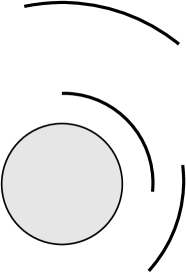
Figure 5: The image of a triply-connected domain under the conformal map $w_{a}(z)$ such that $\tilde{G}(z,a)=-\log|w_{a}(z)|$. The function $w_{a}$ maps the domain onto the exterior of the unit (dashed) circle with $g=3$ concentric circular cuts. Positions and lengths of the arcs depend on the shape of ${\sf{\sf D^{c}}}$ in fig. 3 and depend also on the normalization point $z=a$ which is mapped to $\infty$.

The function $w_{a}(z)$ such that $\tilde{G}(z,a)=-\log|w_{a}(z)|$ maps ${\sf D^{c}}$ onto the exterior of the unit circle which is slit along $g$ concentric circular arcs (see fig. 5). Since the periods of the function $\tilde{G}$ vanish, the function $w_{a}$ is single-valued. Positions of the arcs depend on the shape of ${\sf D^{c}}$ as well as on the point $a$ which is mapped to $\infty$. The radii of the arcs, $R_{\alpha}$, are expressed through the dual tau-function as

$$\log R_{\alpha}^{2}=\partial_{s_{\alpha}}\!\nabla(a)\tilde{F}$$ (4.10)

In particular, for $a=\infty$ we have $\log R_{\alpha}^{2}=\partial_{s_{\alpha}}\!\partial_{\tau_{0}}\tilde{F}$ (cf. eq. (2.20) for the conformal radius).

Relation to multi-support solutions of matrix models.

The partition function of the model, written as an integral over eigenvalues, reads:

$$\begin{array}[]{c}Z_{N}=\frac{1}{N!}\int\exp\left(\sum_{i<j}^{N}\log|z_{i}-z_{j}|^{2}+\frac{1}{\hbar}\sum_{i=1}^{N}U(z_{i})\right)\prod_{j=1}^{N}d^{2}z_{j}\end{array}$$ (4.11)

The matrix model potential $U$ is usually chosen to be of the form

$$\begin{array}[]{c}U(z)=-z\bar{z}+V(z)+\overline{V(z)}\end{array}$$ (4.12)

where $V(z)$ is at the moment some polynomial; however, we will see immediately that the coincidence of the notation with (3.57) is not accidental. The parameter $\hbar$, in the large $N$ limit, tends to zero simultaneously with $N\to\infty$ in such a way that $t_{0}=N\hbar$ is kept finite and fixed. In the leading order, one can apply the saddle point method. The saddle point condition is

$$\hbar\!\sum_{j=1,\neq i}^{N}\frac{1}{z_{i}-z_{j}}+\partial_{z_{i}}U(z_{i})=0$$

The density of eigenvalues is a sum of two-dimensional delta-functions:

$$\rho(z)=\pi\hbar\sum_{i}\delta^{(2)}(z-z_{i})$$

In the large $N$ limit, one treats it as a continuous function normalized as ${1\over\pi}\int\rho(z)d^{2}z=t_{0}$. In terms of the continuous density the saddle point equation reads

$$\begin{array}[]{c}{1\over\pi}\int\frac{\rho(\zeta)d^{2}\zeta}{z-\zeta}+\partial_{z}U(z)=0\end{array}$$ (4.13)

The solution is well known and easy to obtain: the extremal density $\rho_{0}(z)$ is constant in some domain ${\sf D}$ (the support of eigenvalues which can be a union of disconnected domains ${\sf D}_{\alpha}$) and zero otherwise. More precisely,

$$\rho_{0}(z)=\left\{\begin{array}[]{ll}1&z\in{\sf D}\\ 0&z\in{\bf C}\setminus{\sf D}\equiv{\sf D^{c}}\end{array}\right.$$

Note that the saddle point condition is imposed only for $z$ inside the support of eigenvalues. Writing (cf. (3.57))

$$V(z)=\sum_{k=1}^{p}\tau_{k}B_{k}(z)$$

multiplying eq. (4.13) by $A_{k}(z)$ and integrating it over the boundary of the support of eigenvalues, one finds that the domain ${\sf D}$ is such that the coefficients $\tau_{k}$ are moments of its complement with respect to the basis functions $A_{k}$ and the higher moments (with numbers greater than $p$) vanish. As is proven in sect. 3, these conditions, together with the normalization condition for the density, locally determine the shape of the support of eigenvalues. Equivalently, one might parametrize the polynomial as $V(z)=\sum_{k=1}^{p}t_{k}z^{k}$, then $t_{k}$ are moments of the ${\bf C}\setminus{\sf D}$ with respect to the functions $z^{-k}$.

An interesting problem is to obtain, for a given value of $t_{0}$, necessary and sufficient conditions on the polynomial $V$ for the support of eigenvalues to be a union of $g+1$ disconnected domains (”droplets”) with non-zero filling. One may approach this problem from a “classical” limit of very small (point-like) droplets. Clearly, for our choice of the signs in (4.11) and (4.12), the stable point-like droplets are located at minima of $-U(z)$, or equivalently at maxima of $U(z)$. As soon as we use the basis which explicitly depends on the marked points $z_{\alpha}\in{\sf D}_{\alpha}$, it is natural to consider the germ configuration with point-like eigenvalue droplets at the points $z_{\alpha}$. It is easy to see that the sufficient conditions for the potential (4.12) to have maxima at the points $z_{\alpha}$ are

$$\bar{z}_{\alpha}=V^{\prime}(z_{\alpha}),\;\;\;\;|V^{\prime\prime}(z_{\alpha})|<1\;\;\;\mbox{for all $\alpha$}$$ (4.14)

The first one means that there is an extremum of the potential $U(z)$ at the point $z_{\alpha}$. The second one ensures that eigenvalues of the matrix of second derivatives of the potential at the extremum are both negative, i.e. the extremum is actually a maximum of $U(z)$. The first condition literally coincides with the one used in [22] for the completely degenerate curve (point-like droplets) while the second one requires that not all extrema are filled, so that the “smooth” genus $g$ is always less than the maximal possible genus $(p-1)^{2}-1$. Let now $V_{0}(z)$ be a minimal degree polynomial that obeys these conditions. Then perturbed polynomials of the form

$$V(z)=V_{0}(z)+\sum_{k\geq g+2}\tau_{k}B_{k}(z)$$

obey the same conditions for sufficiently small $\tau_{k}$, and this is the advantage of using the basis (3.10), (3.13) from the perspective of matrix models.

The saddle point equation (4.13) just means that the “effective potential” $\frac{1}{\pi}\int_{\sf D}\log|z-\zeta|^{2}d^{2}\zeta+U(z)$ is constant in each ${\sf D}_{\alpha}$, i.e. for $z\in{\sf D}_{\alpha}$ it holds:

$$\begin{array}[]{c}\frac{2}{\pi}\int_{\sf D}\log|z-\zeta|d^{2}\zeta+U(z)=v_{0}+\Pi_{\alpha}\end{array}$$ (4.15)

where $v_{0}=\frac{2}{\pi}\int_{\sf D}\log|z|d^{2}z$, and so in our normalization $\Pi_{0}=0$.

Let $N_{\alpha}$ be the number of eigenvalues in ${\sf D}_{\alpha}$, then $\lim_{N\to\infty}\hbar N_{\alpha}=s_{\alpha}$. First we find the free energy with some fixed $s_{\alpha}$:

$$\left.\lim_{N\to\infty}\left(\hbar^{2}\log Z_{N}\right)\right|_{s_{\alpha}\;{\rm fixed}}={1\over\pi^{2}}\int\!\int\rho_{0}(z)\log|z-\zeta|\rho_{0}(\zeta)d^{2}zd^{2}\zeta+{1\over\pi}\int\rho_{0}(z)U(z)d^{2}z$$

where one should substitute (4.15). The result is

$$\left.\lim_{N\to\infty}\left(\hbar^{2}\log Z_{N}\right)\right|_{s_{\alpha}\;{\rm fixed}}\!=-\,\frac{1}{\pi^{2}}\int_{{\sf D}}\!\int_{{\sf D}}\log|z^{-1}-\zeta^{-1}|d^{2}zd^{2}\zeta+\sum_{\alpha=1}^{g}\Pi_{\alpha}s_{\alpha}=\tilde{F}(s_{\alpha},{\mbox{\boldmath$\tau$}})$$ (4.16)

This quantity depends on $s_{\alpha}$’s. It is given by the value of the integrand in (4.11) at the saddle point with fixed $s_{\alpha}$.

If one wants to take into account the “tunneling” of eigenvalues between different components of the support, $s_{\alpha}$ are no longer free parameters, and the free energy $F^{(0)}$ of the “planar limit” of the matrix model should be obtained by extremizing $\tilde{F}$ with respect to $s_{\alpha}$ (with fixed $t_{0}$). It follows from the above that $\partial_{s_{\alpha}}\tilde{F}=\Pi_{\alpha}$ and so the extremum is at $\Pi_{\alpha}=0$. Therefore,

$$\begin{array}[]{c}\left.\phantom{A/B}F^{(0)}=F\right|_{\Pi_{\alpha}=0}\end{array}$$ (4.17)

where $F$ is given by (2.35). The results of sect. 3 imply that the growth of the support of eigenvalues, when $N\to N+\delta N$ and the tunneling is taken into account, is given by the normal displacement of the boundary proportional to the normal derivative of the Green function with the minus sign, like in (2.9). Since this quantity is always non-negative, we conclude that if a point belongs to the support of eigenvalues, it does so as $t_{0}$ increases. In particular, if one starts with point-like droplets at the points $z_{\alpha}$, as is discussed above, then these points always remain inside the droplets.

Let us note that different aspects of multi-support solutions of the 2-matrix model and matrix models with complex eigenvalues were discussed in [22, 26, 25].

For matrix models one usually restricts oneself to the algebraic case of finite amount of nonvanishing moments playing the role of the coefficients of the matrix model potential (4.12). In such case the corresponding complex curve can be described by an algebraic equation [22], which can be thought of as auxiliary constraint to the second derivatives of $F$. These auxiliary constraints look similar to the reduction conditions in the case of Landau-Ginzburg topological theories (see, for example, discussion of such conditions in the context of dispersionless Hirota equations and WDVV equations in [7]). Their meaning is that the derivatives w.r.t. the times $\{\tau_{k}\}$ for $k>g+1$ (where $g$ is genus of corresponding algebraic complex curve) can be expressed through the derivatives restricted to $k\leq g+1$.

5 Green function on the Schottky double and generalized Hirota equations

Let us now turn to the generalization of the dispersionless Hirota equations to the multiply-connected case.

For a unified treatment of the two “dual” representations of the Dirichlet problem discussed in the two previous sections, we make a simple change of variables. Namely, let us introduce the generic “period” variables $X_{\alpha}$ which are identified either with $\Pi_{\alpha}$ or $2\pi i\,s_{\alpha}$ depending on the choice of the set of cycles, and the function ${\cal F}(X_{\alpha},{\mbox{\boldmath$\tau$}})$ equal to $F(X_{\alpha},{\mbox{\boldmath$\tau$}})$ or $\tilde{F}(\frac{X_{\alpha}}{2\pi i},{\mbox{\boldmath$\tau$}})$ respectively. Then the main relations (3.45) – (3.47) and (4.4) – (4.6) acquire the form

$$\begin{array}[]{c}G(a,b)=\log|a^{-1}-b^{-1}|+\frac{1}{2}\nabla(a)\nabla(b){\cal F}\end{array}$$ (5.1)

$$\omega_{\alpha}(z)=-\,\partial_{\alpha}\nabla(z){\cal F}$$ (5.2)

$$T_{\alpha\beta}=2\pi i\,\partial_{\alpha}\partial_{\beta}{\cal F}$$ (5.3)

where $\partial_{\alpha}:=\partial_{X_{\alpha}}$ and $G$, $\omega$ and $T$ stand for the corresponding objects with or without tilde, depending on the chosen basis of cycles.

We will see below that, in analogy to the simply-conected case, any second order derivative of the function ${\cal F}$ w.r.t. $\tau_{k}$ (and $\bar{\tau}_{k}$), ${\cal F}_{ik}$, will be expressed through the derivatives $\{{\cal F}_{\alpha\beta}\}$ where $\alpha,\beta=0,\ldots,g$ together with $\{{\cal F}_{\alpha\tau_{i}}\}$ and their complex conjugated. To be more precise, one can consider all second derivatives as functions of $\{{\cal F}_{\alpha\beta},{\cal F}_{\alpha k}\}$ modulo certain relations on the latter, like the relation (5.14) to be discussed below. Sometimes on this “small phase space” more extra constraints arise, which can be written in the form similar to the Hirota or WDVV equations [27]; we are not going to discuss this issue here, restricting ourselves to the generic situation.

The Abel map.

To derive equations for the function $F={\cal F}$ in sect. 2, we used the representation (2.23) for the conformal map $w(z)$ in terms of ${\cal F}$ and eq. (1.2) relating the conformal map to the Green function which, in its turn, is expressed through the second order derivatives of ${\cal F}$. In the multiply-connected case, our strategy is basically the same, with the suitable analog of the conformal map $w(z)$ (or rather of $\log w(z)$) being the embedding of ${\sf D^{c}}$ into the $g$-dimensional complex torus ${\bf Jac}$, the Jacobi variety of the Schottky double. This embedding is given, up to an overall shift in ${\bf Jac}$, by the Abel map $z\mapsto{\bf W}(z):=(W_{1}(z),\ldots,W_{g}(z))$ where

$$W_{\alpha}(z)=\int_{\xi_{0}}^{z}dW_{\alpha}$$ (5.4)

is the holomorphic part of the harmonic measure $\omega_{\alpha}$. By virtue of (5.2), the Abel map is represented through the second order derivatives of the function ${\cal F}$:

$$W_{\alpha}(z)-W_{\alpha}(\infty)=\int_{\infty}^{z}dW_{\alpha}=-\partial_{\alpha}D(z){\cal F}$$ (5.5)

$$2\,{\rm Re}\,W_{\alpha}(\infty)=\omega_{\alpha}(\infty)=-\partial_{\tau_{0}}\partial_{\alpha}{\cal F}$$ (5.6)

The last formula immediately follows from (5.2).

The Green function and the prime form.

The Green function of the Dirichlet boundary problem, appearing in (5.1), can be written in terms of the prime form (A.4) on the Schottky double (cf. (1.2)):

$$\begin{array}[]{c}G(z,\zeta)=\log\left|E(z,\zeta)\over E(z,\bar{\zeta})\right|\end{array}$$ (5.7)

Here by $\bar{\zeta}$ we mean the (holomorphic) coordinate of the “mirror” point on the Schottky double, i.e. the “mirror” of $\zeta$ under the antiholomorphic involution. The pairs of such mirror points satisfy the condition $W_{\alpha}(\zeta)+\overline{W_{\alpha}(\bar{\zeta})}=0$ in the Jacobian (i.e., the sum should be zero modulo the lattice of periods). The prime form is written through the Riemann theta functions and the Abel map as follows:

$$E(z,\zeta)=\frac{\theta_{\ast}({\bf W}(z)-{\bf W}(\zeta))}{h(z)\,h(\zeta)}$$ (5.8)

when the both points are on the upper sheet and

$$E(z,\bar{\zeta})=\frac{\theta_{\ast}({\bf W}(z)+\overline{{\bf W}(\zeta)})}{ih(z)\,\overline{h(\zeta)}}$$ (5.9)

when $z$ is on the upper sheet and $\bar{\zeta}$ is on the lower one (for other cases we define $E(\bar{z},\bar{\zeta})=\overline{E(z,\zeta)}$, $E(\bar{z},\zeta)=\overline{E(z,\bar{\zeta})}$). Here $\theta_{\ast}({\bf W})\equiv\theta_{{\mbox{\boldmath$\delta$}}^{\ast}}({\bf W}|T)$ is the Riemann theta function (A.2) with the period matrix $T_{\alpha\beta}=2\pi i\,\partial_{\alpha}\partial_{\beta}{\cal F}$ and any odd characteristics ${\mbox{\boldmath$\delta$}}^{\ast}$, and

$$h^{2}(z)=-z^{2}\sum_{\alpha=1}^{g}\theta_{\ast,\alpha}(0)\partial_{z}W_{\alpha}(z)=z^{2}\sum_{\alpha=1}^{g}\theta_{\ast,\alpha}(0)\sum_{k\geq 1}A_{k}^{\prime}(z)\partial_{\alpha}\partial_{\tau_{k}}{\cal F}$$ (5.10)

Note that in the l.h.s. of (5.9) the bar means the reflection in the double while in the r.h.s. the bar means complex conjugation. The notation is consistent since the local coordinate in the lower sheet is just the complex conjugate one. However, one should remember that $E(z,\bar{\zeta})$ is not obtained from (5.8) by a simple substitution of the complex conjugated argument. On different sheets so defined prime “form” $E$ is represented by different functions. In our normalization (5.9) $iE(z,\bar{z})$ is real (see also Appendix B) and

$$\lim_{\zeta\to z}\frac{E(z,\zeta)}{z^{-1}-\zeta^{-1}}=1$$

In particular, $\lim_{z\to\infty}zE(z,\infty)=1$.

The prime form and the tau-function.

In (5.7), the $h$-functions in the prime forms cancel, so the analog of (2.17) reads

$$\begin{array}[]{c}\log\left|\theta_{\ast}({\bf W}(z)-{\bf W}(\zeta))\over\theta_{\ast}({\bf W}(z)+\overline{\bf W(\zeta)})\right|^{2}=\log\left|{1\over z}-{1\over\zeta}\right|^{2}+\nabla(z)\nabla(\zeta){\cal F}\end{array}$$ (5.11)

This equation already explains the claim made in the beginning of this section. Indeed, the r.h.s. is the generating function for the derivatives ${\cal F}_{ik}$ while the l.h.s. is expressed through derivatives of the form ${\cal F}_{\alpha k}$ and ${\cal F}_{\alpha\beta}$ only. The expansion in powers of $z,\zeta$ allows one to express the former through the latter.

The analogs of eqs. (2.19), (2.20) are, respectively:

$$\log\left|\theta_{\ast}({\bf W}(z)-{\bf W}(\infty))\over\theta_{\ast}({\bf W}(z)+\overline{{\bf W}(\infty)})\right|^{2}=-\log|z|^{2}+\partial_{\tau_{0}}\nabla(z){\cal F}$$ (5.12)

$$\log\left|\frac{h^{2}(\infty)}{\theta_{\ast}({\mbox{\boldmath$\omega$}}(\infty))}\right|^{2}=\partial_{\tau_{0}}^{2}{\cal F}$$ (5.13)

Here ${\mbox{\boldmath$\omega$}}(z)\equiv 2\,{\rm Re}\,{\bf W}(z)=(\omega_{1}(z),\ldots,\omega_{g}(z))$ and

$$h^{2}(\infty)=\lim_{z\to\infty}z\,\theta_{\ast}\left(\int_{\infty}^{z}d{\bf W}\right)=-\sum_{\alpha=1}^{g}\theta_{\ast,\alpha}(0)\partial_{\alpha}\partial_{\tau_{1}}{\cal F}$$

A simple check shows that the l.h.s. of (5.13) can be written as $-2\log(iE(\infty,\bar{\infty}))$. As is seen from the expansion $G(z,\infty)=-\log|z|-\log(iE(\infty,\bar{\infty}))+O(z^{-1})$ as $z\to\infty$, $(iE(\infty,\bar{\infty}))^{-1}$ is a natural analog of the conformal radius, and (5.13) indeed turns to (2.20) in the simply-connected case (see Appendix B for an explicit illustrative example). However, now it provides a nontrivial relation on ${\cal F}_{\alpha\beta}$’s and ${\cal F}_{\alpha i}$’s:

$$\begin{array}[]{c}\left(\sum_{\alpha}\theta_{\ast,\alpha}\partial_{\alpha}\partial_{\tau_{1}}{\cal F}\right)\left(\sum_{\beta}\theta_{\ast,\beta}\partial_{\beta}\partial_{\bar{\tau}_{1}}{\cal F}\right)=\theta^{2}_{\ast}({\mbox{\boldmath$\omega$}}(\infty))e^{\partial_{\tau_{0}}^{2}{\cal F}}\end{array}$$ (5.14)

so that the “small phase space” contains the derivatives modulo this relation.

The next steps are exactly the same as in sect. 2: we are going to decompose these equalities into holomorphic and antiholomorphic parts. The results are conveniently written in terms of the prime form. The counterpart of (2.22) is

$$\log\frac{E(\zeta,z)E(\infty,\bar{\zeta})}{E(\zeta,\infty)E(z,\bar{\zeta})}=\log\left(1-\frac{\zeta}{z}\right)+D(z)\nabla(\zeta){\cal F}$$ (5.15)

Tending $\zeta\to\infty$, we get:

$$\log\frac{E(z,\bar{\infty})}{E(z,\infty)}=\log z+\log E(\infty,\bar{\infty})-\partial_{\tau_{0}}D(z){\cal F}$$ (5.16)

Separating holomorphic and antiholomorphic parts of (5.15) in $\zeta$, we get analogs of (2.24) and (2.25):

$$\log\frac{E(z,\zeta)}{E(z,\infty)E(\infty,\zeta)}=\log(z-\zeta)+D(z)D(\zeta){\cal F}$$ (5.17)

$$-\log\frac{E(z,\bar{\zeta})E(\infty,\bar{\infty})}{E(z,\bar{\infty})E(\infty,\bar{\zeta})}=D(z)\bar{D}(\bar{\zeta}){\cal F}$$ (5.18)

Combining these equalities (with merging points $z\to\zeta$ in particular), one is able to obtain the following representations of the prime form itself:

$$E(z,\zeta)=(z^{-1}-\zeta^{-1})e^{-\frac{1}{2}(D(z)-D(\zeta))^{2}{\cal F}}$$ (5.19)

$$iE(z,\bar{\zeta})=e^{-\frac{1}{2}(\partial_{\tau_{0}}+D(z)+\bar{D}(\bar{\zeta}))^{2}{\cal F}}$$ (5.20)

Note also the nice formula

$$iE(z,\bar{z})=e^{-\frac{1}{2}\nabla^{2}(z){\cal F}}$$ (5.21)

Generalized Hirota relations.

For higher genus Riemann surfaces there are no simple universal relations connecting values of prime forms at different points, which, via (5.19), (5.20), could be used to generate equations on ${\cal F}$. The best available relation [9] is the celebrated Fay identity (A.5). Although it contains not only prime forms but Riemann theta functions themselves, it is really a source of closed equations on ${\cal F}$, since all the ingredients are in fact representable in terms of second order derivatives of ${\cal F}$ in different variables.

An analog of the KP version of the Hirota equation (2.26) for the function ${\cal F}$ can be obtained by plugging eqs. (5.5) and (5.19) into the Fay identity (A.5). As a result, one obtains a closed equation which contains second order derivatives of the ${\cal F}$ only (recall that the period matrix in the theta-functions is essentially the matrix of the derivatives ${\cal F}_{\alpha\beta}$). A few equivalent forms of this equation are available. First, shifting ${\bf Z}\rightarrow{\bf Z}-{\bf W}_{3}+{\bf W}_{4}$ in (A.5) and putting $z_{4}=\infty$, one gets the relation

$$\begin{array}[]{c}(a-b)e^{D(a)D(b){\cal F}}\ \theta\left(\int_{\infty}^{a}d{\bf W}+\int_{\infty}^{b}d{\bf W}-{\bf Z}\right)\ \theta\left(\int_{\infty}^{c}d{\bf W}-{\bf Z}\right)\,+\\ +\,(b-c)e^{D(b)D(c){\cal F}}\ \theta\left(\int_{\infty}^{b}d{\bf W}+\int_{\infty}^{c}d{\bf W}-{\bf Z}\right)\ \theta\left(\int_{\infty}^{a}d{\bf W}-{\bf Z}\right)\,+\\ +\,(c-a)e^{D(c)D(a){\cal F}}\ \theta\left(\int_{\infty}^{c}d{\bf W}+\int_{\infty}^{a}d{\bf W}-{\bf Z}\right)\ \theta\left(\int_{\infty}^{b}d{\bf W}-{\bf Z}\right)\,=0\end{array}$$ (5.22)

The vector ${\bf Z}$ is arbitrary (in particular, zero). We see that (2.26) gets “dressed” by the theta-factors. Each theta-factor is expressed through ${\cal F}$ only. For example,

$$\theta\left(\int_{\infty}^{z}d{\bf W}\right)=\sum_{n_{\alpha}\in{\bf Z}}\exp\left(-2\pi^{2}\sum_{\alpha\beta}n_{\alpha}n_{\beta}\partial_{\alpha\beta}^{2}{\cal F}-2\pi i\sum_{\alpha}n_{\alpha}\partial_{\alpha}D(z){\cal F}\right)$$

Another form of this equation, obtained from (5.22) for a particular choice of ${\bf Z}$, reads

$$(a\!-\!b)c^{-1}e^{\frac{1}{2}(D(a)+D(b))^{2}{\cal F}}h(c)\theta_{\ast}\left(\int_{\infty}^{a}d{\bf W}\!+\!\int_{\infty}^{b}d{\bf W}\right)+[\mbox{cyclic per-s of $a,b,c$}]=0$$ (5.23)

Taking the limit $c\to\infty$ in (5.22), one gets an analog of (2.27):

$$\begin{array}[]{c}1\,-\,{\theta(\int_{\infty}^{a}d{\bf W}+\int_{\infty}^{b}d{\bf W}-{\bf Z})\ \ \theta({\bf Z})\over\theta(\int_{\infty}^{a}d{\bf W}-{\bf Z})\ \theta(\int_{\infty}^{b}d{\bf W}-{\bf Z})}\,e^{D(a)D(b){\cal F}}\,=\\ =\,\frac{D(a)-D(b)}{a-b}\partial_{\tau_{1}}{\cal F}+\frac{1}{a-b}\,\sum_{\alpha=1}^{g}\frac{\partial}{\partial Z_{\alpha}}\log{\theta(\int_{\infty}^{a}d{\bf W}-{\bf Z})\over\theta(\int_{\infty}^{b}{\bf W}-{\bf Z})}\,\partial_{\alpha}\partial_{\tau_{1}}{\cal F}\end{array}$$ (5.24)

which also follows from another Fay identity (A.6).

Equations on ${\cal F}$ with $\bar{\tau}_{k}$-derivatives follow from the general Fay identity (A.5) with some points on the lower sheet. Besides, many other equations can be derived as various combinations and specializations of the ones mentioned above. Altogether, they form an infinite hierarchy of consistent differential equations of a very complicated structure which deserves further investigation. The functions ${\cal F}$ corresponding to different choices of independent variables (i.e., to different bases in homology cycles on the Schottky double) provide different solutions to this hierarchy.

Higher genus analogs of the dispersionless Toda equation.

Let us show how the simplest equation of the hierarchy, the dispersionless Toda equation (2.30), is modified in the multiply-connected case. Applying $\partial_{z}\partial_{\bar{\zeta}}$ to both sides of (5.18) and setting $\zeta=z$, we get:

$$(\partial D(z))(\bar{\partial}\bar{D}(\bar{z})){\cal F}=-\partial_{z}\partial_{\bar{z}}\log E(z,\bar{z})$$

Here $\partial D(z)$ is the $z$-derivative of the operator $D(z)$: $\partial D(z)=\sum_{k}A^{\prime}_{k}(z)\partial_{\tau_{k}}$. To transform the r.h.s., we use the identity (A.8) (Appendix A) and specialize it to the particular local parameters on the two sheets:

$$|z|^{4}\partial_{z}\partial_{\bar{z}}\log E(z,\bar{z})=\frac{\theta({\mbox{\boldmath$\omega$}}(z)+{\bf Z})\theta({\mbox{\boldmath$\omega$}}(z)-{\bf Z})}{\theta^{2}({\bf Z})E^{2}(z,\bar{z})}+|z|^{4}\sum_{\alpha,\beta}(\log\theta({\bf Z}))_{,\,\alpha\beta}\,\partial_{z}W_{\alpha}(z)\partial_{\bar{z}}\overline{W_{\beta}(z)}$$

Tending $z$ to $\infty$, we obtain a family of equations (parametrized by an arbitrary vector ${\bf Z}$) which generalize the dispesrionless Toda equation for the tau-function:

$$\partial_{\tau_{1}}\partial_{\bar{\tau}_{1}}{\cal F}=\frac{\theta({\mbox{\boldmath$\omega$}}(\infty)\!+\!{\bf Z})\theta({\mbox{\boldmath$\omega$}}(\infty)\!-\!{\bf Z})}{\theta^{2}({\bf Z})}\,e^{\partial_{\tau_{0}}^{2}{\cal F}}\,-\!\!\sum_{\alpha,\beta=1}^{g}\!(\log\theta({\bf Z}))_{,\,\alpha\beta}\,(\partial_{\alpha}\partial_{\tau_{1}}{\cal F})(\partial_{\beta}\partial_{\bar{\tau}_{1}}{\cal F})$$ (5.25)

(Here we used the $z\to\infty$ limits of (5.5) and (5.21).) The following two equations correspond to special choices of the vector ${\bf Z}$:

$$\begin{array}[]{c}\partial_{\tau_{1}}\partial_{\bar{\tau}_{1}}{\cal F}+\sum_{\alpha,\beta=1}^{g}(\log\theta(0))_{,\,\alpha\beta}\,(\partial_{\alpha}\partial_{\tau_{1}}{\cal F})(\partial_{\beta}\partial_{\bar{\tau}_{1}}{\cal F})=\frac{\theta^{2}({\mbox{\boldmath$\omega$}}(\infty))}{\theta^{2}(0)}\ e^{\partial_{\tau_{0}}^{2}{\cal F}}\end{array}$$ (5.26)

$$\begin{array}[]{c}\partial_{\tau_{1}}\partial_{\bar{\tau}_{1}}{\cal F}=-\sum_{\alpha,\beta=1}^{g}\left[\log\theta_{\ast}({\mbox{\boldmath$\omega$}}(\infty))\right]_{,\alpha\beta}(\partial_{\alpha}\partial_{\tau_{1}}{\cal F})(\partial_{\beta}\partial_{\bar{\tau}_{1}}{\cal F})\end{array}$$ (5.27)

Finally, let us specify the equation (5.25) for the genus $g=1$ case. In this case there is only one extra variable $X:=X_{1}$ ($\Pi_{1}$ or $2\pi is_{1}$). The Riemann theta-function $\theta({\mbox{\boldmath$\omega$}}(\infty)+{\bf Z})$ is then replaced by the Jacobi theta-function $\vartheta\left(\left.\partial_{X}\partial_{\tau_{0}}{\cal F}-Z\right|T\right)\equiv\vartheta_{3}\left(\left.\partial_{X}\partial_{\tau_{0}}{\cal F}-Z\right|T\right)$, where the elliptic modular parameter is $T=2\pi i\,\partial_{X}^{2}{\cal F}$, and the vector $Z\equiv{\bf Z}$ has only one component. The equation has the form:

$$\begin{array}[]{c}\displaystyle{\partial_{\tau_{1}}\partial_{\bar{\tau}_{1}}{\cal F}=\frac{\vartheta_{3}\left(\left.\partial_{X}\partial_{\tau_{0}}{\cal F}\!+\!Z\right|2\pi i\,\partial_{X}^{2}{\cal F}\right)\vartheta_{3}\left(\left.\partial_{X}\partial_{\tau_{0}}{\cal F}\!-\!Z\right|2\pi i\,\partial_{X}^{2}{\cal F}\right)}{\vartheta_{3}^{2}\left(\left.Z\right|2\pi i\,\partial_{X}^{2}{\cal F}\right)}\,e^{\partial_{\tau_{0}}^{2}{\cal F}}}\\ \\ \displaystyle{-\,\,\partial_{Z}^{2}\log\vartheta_{3}\left(\left.Z\right|2\pi i\,\partial_{X}^{2}{\cal F}\right)\,(\partial_{X}\partial_{\tau_{1}}{\cal F})(\partial_{X}\partial_{\bar{\tau}_{1}}{\cal F})}\end{array}$$ (5.28)

Note also that equation (5.14) acquires the form

$$(\partial_{X}\partial_{\tau_{1}}{\cal F})(\partial_{X}\partial_{\bar{\tau}_{1}}{\cal F})=\left(\frac{\vartheta_{1}\left(\left.\partial_{X}\partial_{\tau_{0}}{\cal F}\right|2\pi i\,\partial_{X}^{2}{\cal F}\right)}{\vartheta_{1}^{\prime}\left(\left.0\right|2\pi i\,\partial_{X}^{2}{\cal F}\right)}\right)^{2}e^{\partial_{\tau_{0}}^{2}{\cal F}}$$ (5.29)

where $\vartheta_{\ast}\equiv\vartheta_{1}$ is the only odd Jacobi theta-function. Combining (5.28) and (5.29) one may also write the equation

$$\begin{array}[]{c}\partial_{\tau_{1}}\partial_{\bar{\tau}_{1}}{\cal F}=\left[\frac{\vartheta_{3}\left(\left.\partial_{X}\partial_{\tau_{0}}{\cal F}\!+\!Z\right|2\pi i\,\partial_{X}^{2}{\cal F}\right)\vartheta_{3}\left(\left.\partial_{X}\partial_{\tau_{0}}{\cal F}\!-\!Z\right|2\pi i\,\partial_{X}^{2}{\cal F}\right)}{\vartheta_{3}^{2}\left(\left.Z\right|2\pi i\,\partial_{X}^{2}{\cal F}\right)}\right.\\ \left.-\,\,\left(\frac{\vartheta_{1}\left(\left.\partial_{X}\partial_{\tau_{0}}{\cal F}\right|2\pi i\,\partial_{X}^{2}{\cal F}\right)}{\vartheta_{1}^{\prime}\left(\left.0\right|2\pi i\,\partial_{X}^{2}{\cal F}\right)}\right)^{2}\partial_{Z}^{2}\log\vartheta_{3}\left(\left.Z\right|2\pi i\,\partial_{X}^{2}{\cal F}\right)\right]\,e^{\partial_{\tau_{0}}^{2}{\cal F}}\end{array}$$ (5.30)

whose form is close to (2.30) but differs by the nontrivial “coefficient” in the square brackets. In the limit $T\to i\infty$ the theta-function $\vartheta_{3}$ tends to unity, and we obtain the dispersionless Toda equation (2.30).

6 Conclusions

In this paper we have considered the Dirichlet boundary problem in planar multiply-connected domains. A planar multiply-connected domain ${\sf D^{c}}$ is the complex plane with several holes. We study how the solution of the Dirichlet problem depends on small deformations of boundaries of the holes.

General properties of such deformations allow us to introduce the quasiclassical tau-function associated to the variety of planar multiply-connected domains. By the tau-function, we actually mean its logarithm, which only makes sense for the quasiclassical or Whitham-type integrable hierarchies. Namely, the key properties are the specific “exchange” relations (3.43) which follow from the Hadamard variational formula for the Green function and the harmonic measure. They have the form of integrability conditions and thus ensure the existence of the tau-function. The tau-function corresponds to a particular solution of the universal Whitham hierarchy [4] and generalizes the dispersionless tau-function which describes deformations of simply-connected domains.

The algebro-geometric data associated with the multiply-connected geometry include a Riemann surface with antiholomorphic involution, the Schottky double of the domain ${\sf D^{c}}={\bf C}\setminus{\sf D}$ endowed with particular holomorphic coordinates $z$ and ${\bar{z}}$ on the two sheets of the double, respecting the involution. This Riemann surface has genus $g=\#\{{\rm holes}\}-1$. The (logarithm of) tau-function, ${\cal F}$, describes small deformations of these data as functions of an infinite set of independent deformation parameters which are basically harmonic moments of the domain. These variables can be equivalently redefined as periods of the generating one-form $S(z)dz$ over non-trivial cycles on the double and the residues of the one-forms $A_{k}(z)S(z)dz$, where $A_{k}(z)\ \mathrel{\mathop{\simeq}\limits_{z\to\infty}}\ z^{-k}$ is some proper global basis (3.10) of harmonic functions.

We have obtained simple expressions for the period matrix, the Abel map and the prime form on the Schottky double in terms of the function ${\cal F}$. Specifically, all these objects are expressed through second order derivatives of the ${\cal F}$ in its independent variables.

The generalized dispersionless Hirota equations on ${\cal F}$ for the multiply-connected case (equivalent to the Whitham hierarchy) are obtained by incorporating the above mentioned expressions into the Fay identities. As a result, one comes to a series of quite non-trivial equations for (second derivatives of) the function $F$, which have not been written before (except for certain relations for the second derivatives of the Seiberg-Witten prepotential [28]). When the Riemann surface degenerates to the Riemann sphere with two marked points, they turn into Hirota equations of the dispersionless Toda hierarchy.

Algebraic orbits of the universal Whitham hierarchy describe the class of domains which can be obtained as conformal images of a “half” of a complex algebraic curve with the antiholomorphic involution under conformal maps given by rational functions on the curve. In particular, all domains having only a finite amount of non-vanishing harmonic moments, are in this class. In this case one can define the curve by a polynomial equation written explicitly in [22]. This situation is an analog of the (Laurent) polynomial conformal maps in the simply-connected case and literally corresponds to multi-support solutions of matrix models with polynomial potentials. The definition of the tau-function for multiply-connected domains proposed above holds in a broader set-up of general algebraic domains. It does not rely on the finitness of the amount of non-vanishing moments. In general any effective way to describe the complex curve associated to a multiply-connected domain by a system of polynomial or algebraic equations is not known. The curve may be thought of as a spectral curve corresponding to a generic finite-gap solution to the Toda lattice hierarchy.

Appendix A. Theta functions and Fay identities

Here we present some definitions and useful formulas from [9]. The Riemann theta function $\theta({\bf W})\equiv\theta({\bf W}|T)$ is defined as

$$\begin{array}[]{c}\theta({\bf W})=\sum_{{\bf n}\in{\bf Z}^{g}}e^{i\pi{\bf n}\cdot T\cdot{\bf n}+2\pi i{\bf n}\cdot{\bf W}}\end{array}$$ (A.1)

The theta function with a (half-integer) characteristics ${\mbox{\boldmath$\delta$}}=({\mbox{\boldmath$\delta$}}_{1},{\mbox{\boldmath$\delta$}}_{2})$, where $\delta_{\alpha}=T_{\alpha\beta}\delta_{1,\beta}+\delta_{2,\alpha}$ and ${\mbox{\boldmath$\delta$}}_{1},{\mbox{\boldmath$\delta$}}_{2}\in\frac{1}{2}{\bf Z}^{g}$ is

$$\begin{array}[]{c}\theta_{{\mbox{\boldmath$\delta$}}}({\bf W})=e^{i\pi{\mbox{\boldmath$\delta$}}_{1}\cdot T\cdot{\mbox{\boldmath$\delta$}}_{1}+2\pi i{\mbox{\boldmath$\delta$}}_{1}\cdot({\bf W}+{\mbox{\boldmath$\delta$}}_{2})}\theta({\bf W}+{\mbox{\boldmath$\delta$}})=\sum_{{\bf n}\in{\bf Z}^{g}}e^{i\pi({\bf n}+{\mbox{\boldmath$\delta$}}_{1})\cdot T\cdot({\bf n}+{\mbox{\boldmath$\delta$}}_{1})+2\pi i({\bf n}+{\mbox{\boldmath$\delta$}}_{1})\cdot({\bf W}+{\mbox{\boldmath$\delta$}}_{2})}\end{array}$$ (A.2)

Under shifts by a period of the lattice, it transforms according to

$$\begin{array}[]{c}\theta_{\mbox{\boldmath$\delta$}}({\bf W}+{\bf e}_{\alpha})=e^{2\pi i\delta_{1,\alpha}}\theta_{\mbox{\boldmath$\delta$}}({\bf W})\\ \theta_{\mbox{\boldmath$\delta$}}({\bf W}+T_{\alpha\beta}{\bf e}_{\beta})=e^{-2\pi i\delta_{2,\alpha}-i\pi T_{\alpha\alpha}-2\pi iW_{\alpha}}\theta_{\mbox{\boldmath$\delta$}}({\bf W})\end{array}$$ (A.3)

The prime form $E(z,\zeta)$ is defined as

$$\begin{array}[]{c}E(z,\zeta)={\theta_{\ast}({\bf W}(z)-{\bf W}(\zeta))\over\sqrt{\sum_{\alpha}\theta_{\ast,\alpha}dW_{\alpha}(z)}\sqrt{\sum_{\beta}\theta_{\ast,\beta}dW_{\beta}(\zeta)}}\end{array}$$ (A.4)

where $\theta_{\ast}$ is any odd theta function, i.e., the theta function with any odd characteristic ${\mbox{\boldmath$\delta$}}^{\ast}$ (the characteristics is odd if $4{\mbox{\boldmath$\delta$}}_{1}^{\ast}\cdot{\mbox{\boldmath$\delta$}}_{2}^{\ast}={\rm odd}$). The prime form does not depend on the particular choice of the odd characteristics. In the denominator,

$$\left.\theta_{\ast,\alpha}=\theta_{\ast,\alpha}(0)=\frac{\partial\theta_{\ast}({\bf W})}{\partial W_{\alpha}}\right|_{{\bf W}=0}$$

is the set of $\theta$-constants.

The data we use in the main text contain also a distinguished coordinates on a Riemann surface: the holomorphic co-ordinates $z$ and $\bar{z}$ on two different sheets, and we do not distinguish, unless it is nessesary between the prime form (A.4) and a function $E(z,\zeta)\equiv E(z,\zeta)(dz)^{1/2}(d\zeta)^{1/2}$ “normalized” onto the differentials of distinguished co-ordinate.

Let us now list the Fay identities [9] used in the paper. The basic one is Fay’s trisecant formula (equation (45) from p. 34 of [9])

$$\begin{array}[]{c}\theta({\bf W}_{1}-{\bf W}_{3}-{\bf Z})\ \theta({\bf W}_{2}-{\bf W}_{4}-{\bf Z})\ E(z_{1},z_{4})E(z_{3},z_{2})\\ +\,\,\theta({\bf W}_{1}-{\bf W}_{4}-{\bf Z})\ \theta({\bf W}_{2}-{\bf W}_{3}-{\bf Z})\ E(z_{1},z_{3})E(z_{2},z_{4})\\ =\,\,\theta({\bf W}_{1}+{\bf W}_{2}-{\bf W}_{3}-{\bf W}_{4}-{\bf Z})\ \theta({\bf Z})\ E(z_{1},z_{2})E(z_{3},z_{4})\end{array}$$ (A.5)

Here ${\bf W}_{i}\equiv{\bf W}(z_{i})$. This identity holds for any four points $z_{1},\dots,z_{4}$ on a Riemann surface and any vector ${\bf Z}\in{\bf Jac}$. In the limit $z_{3}\to z_{4}\equiv\infty$ one gets (formula (38) from p. 25 of [9])

$$\begin{array}[]{c}{\theta(\int_{\infty}^{z_{1}}d{\bf W}+\int_{\infty}^{z_{2}}d{\bf W}-{\bf Z})\ \theta({\bf Z})\over\theta(\int_{\infty}^{z_{1}}d{\bf W}-{\bf Z})\ \theta(\int_{\infty}^{z_{2}}d{\bf W}-{\bf Z})}{E(z_{1},z_{2})\over E(z_{1},\infty)E(z_{2},\infty)}\\ =\,\,d\Omega^{(z_{1},z_{2})}(\infty)+\sum_{\alpha=1}^{g}dW_{\alpha}(\infty)\,\,\partial_{Z_{\alpha}}\!\log\ {\theta(\int_{\infty}^{z_{1}}d{\bf W}-{\bf Z})\over\theta(\int_{\infty}^{z_{2}}d{\bf W}-{\bf Z})}\end{array}$$ (A.6)

where

$$\begin{array}[]{c}d\Omega^{(z_{1},z_{2})}(\infty)=d_{z}\log\ {E(z,z_{1})\over E(z,z_{2})}\end{array}$$ (A.7)

is the normalized Abelian differential of the third kind with simple poles at $z_{1}$ and $z_{2}$ and residues $\pm 1$.

Another relation from [9] we use (see e.g. (29) on p.20 and (39) on p.26) is

$$\begin{array}[]{c}{\theta({\bf W}_{1}-{\bf W}_{2}-{\bf Z})\theta({\bf W}_{1}-{\bf W}_{2}+{\bf Z})\over\theta^{2}({\bf Z})E^{2}(z_{1},z_{2})}=\omega(z_{1},z_{2})+\sum_{\alpha,\beta=1}^{g}\left(\log\theta({\bf Z})\right)_{,\alpha\beta}dW_{\alpha}(z_{1})dW_{\beta}(z_{2})\end{array}$$ (A.8)

where

$$(\log\theta({\bf Z}))_{,\,\alpha\beta}=\frac{\partial^{2}\log\theta({\bf Z})}{\partial Z_{\alpha}\partial Z_{\beta}}$$

and

$$\begin{array}[]{c}\omega(z_{1},z_{2})=d_{z_{1}}d_{z_{2}}\log E(z_{1},z_{2})\end{array}$$ (A.9)

is the canonical bi-differential of the second kind with the double pole at $z_{1}=z_{2}$.

Appendix B. Degenerate Schottky double

For an illustrative purpose we would like to adopt some of the above formulas to the simplest possible case, which is the Riemann sphere realized as the Schottky double of the complement to the disk of radius $r$. In this case

$$\begin{array}[]{c}dW={dz\over z}=id\varphi=-{d{\bar{z}}\over\bar{z}}\end{array}$$ (B.1)

is purely imaginary on the circle and obviously satisfies the condition $dW(z)+\overline{dW(\bar{z})}=0$. Further, (cf. (3.65))

$$\begin{array}[]{c}W(z)=\int_{\xi_{0}}^{z}dW=\int_{r}^{z}dW=\log{z\over r}\end{array}$$ (B.2)

and

$$\begin{array}[]{c}w(z)=e^{W(z)}={z\over r}\end{array}$$ (B.3)

which is nothing but the conformal map of the exterior of the circle $|z|\geq r$ onto exterior of the unit circle $|w|\geq 1$. Note that on the “lower” sheet of the double

$$\begin{array}[]{c}W(\bar{z})=\int_{r}^{\bar{z}}dW=\log{r\over\bar{z}}\end{array}$$ (B.4)

and instead of (B.3) one gets

$$\begin{array}[]{c}w(\bar{z})={r\over\bar{z}}\end{array}$$ (B.5)

which is the conformal map of the exterior of the disk $|\bar{z}|\geq r$ on the lower sheet onto the interior of the unit circle $|w|\leq 1$. The prime form on the genus zero Riemann surface is (cf. (A.4))

$$\begin{array}[]{c}E(z_{1},z_{2})={w_{1}-w_{2}\over\sqrt{dw_{1}}\sqrt{dw_{2}}}\end{array}$$ (B.6)

where $w_{i}\equiv w(z_{i})$. Let us compute $E(\infty,\bar{\infty})$, which is understood in the main text, as “normalized” on the values of the local coordinates $z_{\infty}=1/z$ and $\bar{z}_{\infty}=1/\bar{z}$ in the points $\infty$ and $\bar{\infty}$ on two sheets of the double. One gets (cf. (5.9))

$$\begin{array}[]{c}E^{2}(\infty,\bar{\infty})=-{(w(\infty)-w(\bar{\infty}))^{2}\over(dw(\infty)/dz_{\infty})(dw(\bar{\infty})/dz_{\bar{\infty}})}\end{array}$$ (B.7)

Substituting into (B.7) the formulas (B.3), (B.5) and

$$\begin{array}[]{c}dw(\infty)=\lim_{z\to\infty}{dz\over r}=-\lim_{z\to\infty}{z^{2}\over r}\ dz_{\infty}\\ dw(\bar{\infty})=r\ dz_{\bar{\infty}}\end{array}$$ (B.8)

one finally gets

$$\begin{array}[]{c}E(\infty,\bar{\infty})^{2}=\lim_{z\to\infty}{z^{2}/r^{2}\over(z^{2}/r)r}={1\over r^{2}}\end{array}$$ (B.9)

and this demonstrates that (5.14) indeed turns into (2.20) in the limit.

References

- [1] A. Hurwitz and R. Courant, Vorlesungen über allgemeine Funktionentheorie und elliptische Funktionen. Herausgegeben und ergänzt durch einen Abschnitt über geometrische Funktionentheorie, Springer-Verlag, 1964 (Russian translation, adapted by M.A. Evgrafov: Theory of functions, Nauka, Moscow, 1968).
- [2] A. Marshakov, P. Wiegmann and A. Zabrodin, Commun. Math. Phys. 227 (2002) 131, e-print archive: hep-th/0109048.
- [3] I.M. Krichever, Funct. Anal. Appl. 22 (1989) 200-213
- [4] I.M. Krichever, Commun. Pure. Appl. Math. 47 (1994) 437, e-print archive: hep-th/9205110.
- [5] M. Mineev-Weinstein, P.B. Wiegmann and A. Zabrodin, Phys. Rev. Lett. 84 (2000) 5106, e-print archive: nlin.SI/0001007.
- [6] P.B. Wiegmann and A. Zabrodin, Commun. Math. Phys. 213 (2000) 523, e-print archive: hep-th/9909147.
- [7] A. Boyarsky, A. Marshakov, O. Ruchayskiy, P. Wiegmann and A. Zabrodin, Phys. Lett. B515 (2001) 483-492, e-print archive: hep-th/0105260.
- [8] I. Krichever and S. Novikov, Funct. Anal. Appl. 21 (1987) No 2 46-63.
- [9] J.D.Fay, “Theta Functions on Riemann Surfaces”, Lect. Notes in Mathematics 352, Springer-Verlag, 1973.
- [10] J. Hadamard, Mém. présentés par divers savants à l’Acad. sci., 33 (1908).
- [11] P.J. Davis, The Schwarz function and its applications, The Carus Mathematical Monographs, No. 17, The Math. Assotiation of America, Buffalo, N.Y., 1974.
- [12] I. Krichever, 2000, unpublished.
- [13] L. Takhtajan, Lett. Math. Phys. 56 (2001) 181-228, e-print archive: math.QA/0102164.
- [14] I.K. Kostov, I.M. Krichever, M. Mineev-Weinstein, P.B. Wiegmann and A. Zabrodin, -function for analytic curves, Random matrices and their applications, MSRI publications, 40, Cambridge Academic Press, 2001, e-print archive: hep-th/0005259.
- [15] E. Hille, Analytic function theory, v.II, Ginn and Company, 1962.
-
[16]
J. Gibbons and Y. Kodama, Proceedings of NATO ASI “Singular
Limits of Dispersive Waves”, ed. N. Ercolani,
London – New York, Plenum, 1994;
R. Carroll and Y. Kodama, J. Phys. A: Math. Gen. A28 (1995) 6373. - [17] K. Takasaki and T. Takebe, Rev. Math. Phys. 7 (1995) 743-808.
- [18] M. Schiffer and D.C. Spencer, Functionals of finite Riemann surfaces, Princeton University Press, 1954
- [19] B. Gustafsson, Acta Applicandae Mathematicae 1 (1983) 209-240.
-
[20]
D. Aharonov and H. Shapiro,
J. Anal. Math. 30 (1976) 39-73;
H. Shapiro, The Schwarz function and its generalization to higher dimensions, University of Arkansas Lecture Notes in the Mathematical Sciences, Volume 9, W.H. Summers, Series Editor, A Wiley-Interscience Publication, John Wiley and Sons, 1992. - [21] P. Etingof and A. Varchenko, Why does the boundary of a round drop becomes a curve of order four, University Lecture Series, 3, American Mathematical Society, Providence, RI, 1992.
- [22] V. Kazakov and A. Marshakov, J. Phys. A: Math. Gen. 36 (2003) 3107-3136, e-print archive: hep-th/0211236.
- [23] B. De Wit and A. Marshakov, Theor. Math. Phys. 129 (2001) 1504 [Teor. Mat. Fiz. 129 (2001) 230], e-print archive: hep-th/0105289.
- [24] F. Gakhov, The boundary value problems, Nauka, Moscow, 1977 (in Russian).
- [25] B.Eynard, Large N expansion of the 2-matrix model, multicut case, e-print archive: math-ph/0307052
- [26] M.Bertola, Free energy of the two-matrix model/dToda tau-function, e-print archive: hep-th/0306184
-
[27]
A. Marshakov, A. Mironov and A. Morozov,
Phys. Lett. B389 (1996) 43-52, e-print archive: hep-th/9607109;
H. Braden and A. Marshakov, Phys. Lett. B541 (2002) 376-383, e-print archive: hep-th/0205308. - [28] A. Gorsky, A. Marshakov, A. Mironov and A. Morozov, Nucl. Phys. B527 (1998) 690-716, e-print archive: hep-th/9802007.