INSTANTONS AND CONSTITUENT MONOPOLES INLO-PUB-12/03

Abstract

We review how instanton solutions at finite temperature can be seen as boundstates of constituent monopoles, discuss some speculations concerning their physical relevance and the lattice evidence for their presence in a dynamical context.

11.10.Wx; 12.38.Lg; 14.80.Hv

1 Introduction

Over the last five years there has been a revived interest in studying instantons at finite temperature $T$, so-called calorons [1, 2]. The main reason is that new explicit solutions could be obtained in the case where the Polyakov loop at spatial infinity is non-trivial, necessary to reveal more clearly the constituent nature of these calorons. This asymptotic value of the Polyakov loop is called the holonomy. In gauge theories trivial holonomy, for which the asymptotic value of the Polyakov loop takes values in the center of the gauge group, is typical for the deconfined phase. Therefore, caloron solutions with non-trivial holonomy are more expected to play a role in the confined phase, still at finite temperature, but where the average of the trace of the Polyakov loop is small. In the introduction we start with a pedagogical overview discussing monopoles, instantons, and their physical significance. The next section discusses the construction of the caloron solutions. Secs. 2.1 and 2.2 are more technical, but tutorial in nature. One could skip in particular Secs. 2.3 and 2.4, describing in Sec. 3 the properties of the solutions in less technical terms. Lattice evidence for the dynamical significance of constituent monopoles is discussed in Sec. 4.

1.1 Monopoles

That monopoles should play a role in describing the constituent nature of calorons is in itself not really a surprise, because at finite temperature $A_{0}$ plays in some sense the role of a Higgs field in the adjoint representation. However, a gauge transformation,

$${}^{g}A_{\mu}(x)=g(x)A_{\mu}(x)g^{-1}(x)+g(x)\partial_{\mu}g^{-1}(x),$$ (1)

shows that $A_{0}$ does not transform correctly (unless the gauge transformation is time independent), due to the inhomogeneous term. Instead, the Polyakov loop

$$P(t,\vec{x})={\rm Pexp}\left(\int_{0}^{\beta}A_{0}(t+s,\vec{x})ds\right),$$ (2)

transforms as it should, ${}^{g}P(x)=g(x)P(x)g^{-1}(x)$. Here $\beta=1/kT$ is the period in the imaginary time direction, under which the gauge field is assumed to be periodic. We also will consider other gauges, where $A_{\mu}(x)$ is periodic up to a gauge transformation, in which case the expression for $P$ has to be modified accordingly [3]. For example, in the so-called algebraic gauge, $A_{0}(x)$ is transformed to zero at spatial infinity. In this case the gauge fields satisfy the boundary condition (${{\cal P}_{\infty}}$ to be defined below)

$$A_{\mu}(t+\beta,\vec{x})={{\cal P}_{\infty}}A_{\mu}(t,\vec{x}){\cal{P}}_{\infty}^{-1}.$$ (3)

We will require that the total Euclidean action of these calorons is finite, such that the field strength

$$F_{\mu\nu}(x)=\partial_{\mu}A_{\nu}(x)-\partial_{\nu}A_{\mu}(x)+[A_{\mu}(x),A_{\nu}(x)]$$ (4)

has to go to zero at spatial infinity. It is this that forces the Polyakov loop to become constant at spatial infinity. For SU($n$) gauge theory this gives

$${{\cal P}_{\infty}}\!=\!\exp(\beta A_{0}^{\infty})\!\equiv\!\lim_{|\vec{x}|\to\infty}\!\!P(x),\quad A_{0}^{\infty}\!\equiv\!\frac{2\pi i}{\beta}U_{0}{\rm diag}\left(\mu_{1},\mu_{2},\ldots,\mu_{n}\right)U_{0}^{-1}\!,$$ (5)

independent of the direction and time. Unlike for a Higgs field, however, ${{\cal P}_{\infty}}$ is unitary with determinant 1. Choosing $U_{0}$ (the constant gauge function that brings ${{\cal P}_{\infty}}$ to its diagonal form) appropriately, the $n$ eigenvalues, $\exp(2\pi i\mu_{m})$, are ordered. The freedom in adding an arbitrary integer to $\mu_{m}$ is fixed by ordering the $\mu_{m}$ themselves, and requiring their sum to vanish,

$$\mbox{$\sum_{i=1}^{n}\mu_{i}=0$},\quad\mu_{1}\leq\mu_{2}\leq\ldots\leq\mu_{n}\leq\mu_{n+1}\equiv 1+\mu_{1}.$$ (6)

For trivial holonomy ${{\cal P}_{\infty}}$ is an element of the center of the gauge group, ${{\cal P}_{\infty}}=\exp(2\pi iq/n)\Eins_{n}$ with $q$ an integer between 0 and $n-1$, hence $\mu_{m}=q/n$.

One might now immediately object that a Higgs field that goes to a constant at infinity does not have the usual hedgehog form expected for a non-Abelian ’t Hooft-Polyakov monopole [4], but this is because the caloron solutions are actually such that the total magnetic charge vanishes. The force stability of these solutions is based, as for exact multi-monopole solutions in the Bogomol’ny-Prasad-Sommerfeld (BPS) limit [5] on balancing the electromagnetic with the scalar (Higgs) force [6, 7]. For the caloron the difference is in interchanging repulsive and attractive forces. For a single caloron with topological charge one, this is because there are $n-1$ monopoles with a unit magnetic charge in the $i$-th U(1) subgroup, all compensated by the $n$-th monopole of so-called type $(1,1,\ldots,1)$, having a magnetic charge in each of these subgroups. This special monopole is also called a Kaluza-Klein (KK) monopole [8], as will be explained below. The well-known Harrington-Shepard solution [1] has trivial holonomy, and although all eigenvalues of ${{\cal P}_{\infty}}$ are equal, such that there is no spontaneous symmetry breaking, one still finds a genuine BPS monopole [9] in a suitable limit (it will be the KK monopole that survives).

In a Higgs theory, switching off the Higgs potential and splitting off a square in the energy density,

$$-{\rm Tr}\left((D_{i}\Phi)^{2}+B_{i}^{2}\right)=-{\rm Tr}(D_{i}\Phi\mp B_{i})^{2}\mp 2{\rm Tr}\left(B_{i}D_{i}\Phi\right),$$ (7)

exact monopole solutions are constructed using the BPS condition [5], which imposes the covariant derivative of the Higgs field $\Phi$ to be equal (up to a sign) to the magnetic field, $D_{i}\Phi\equiv\partial_{i}\Phi+[A_{i},\Phi]=\pm B_{i}$, where $B_{i}\equiv{\scriptstyle{{1\over 2}}}\varepsilon_{ijk}F_{jk}$. One is then left with a total derivative

$${\rm Tr}\left(B_{i}D_{i}\Phi\right)={\rm Tr}\left(D_{i}(B_{i}\Phi)\right)=\partial_{i}{\rm Tr}(B_{i}\Phi),$$ (8)

whose integral is proportional to the magnetic charge. The integral can also be associated to the mapping degree of the map $\hat{x}\to\Phi(r\hat{x})$ ($\hat{x}\equiv\vec{x}/|\vec{x}|$) for $r\to\infty$. With $\Phi$ taking values in the algebra, and of fixed length at infinity, this gives for SU(2) a map from $S^{2}$ to $S^{2}$. For a caloron the BPS condition is simply a consequence of the self-duality conditions characteristic of instanton solutions, $E_{i}=D_{i}A_{0}-\partial_{0}A_{i}=\pm B_{i}$, with $\Phi=A_{0}$. One might thus be tempted to call the constituents dyons, rather than monopoles. In the Higgs model the Julia-Zee dyons are constructed by taking $A_{0}$ proportional to the Higgs field $\Phi$ [10]. By a time dependent gauge transformation $A_{0}$ can then be gauged to zero. The resulting electric field is now given by $E_{i}=-\partial_{0}A_{i}$ and is not quantized (and in particular not equal to $\pm B_{i}$). In pure gauge theory it makes, however, no sense to separate $D_{i}\Phi=D_{i}A_{0}$ from $\partial_{0}A_{i}$. Gauge invariance requires that they occur in the combination $F_{i0}=D_{i}A_{0}-\partial_{0}A_{i}$. The electric field is necessarily fixed and quantized as soon as we interpret $A_{0}$ as the Higgs field. As discussed in Ref. [11] adding a fifth dimension for Minkowski time, compactifying the Euclidean time direction to zero size ($\beta\to 0$) allows one to have electric charge as for the Julia-Zee dyon. A compactified Euclidean direction is what one also considers in Kaluza-Klein theories. It is in this sense that the type $(1,1,\ldots,1)$ monopole is called a KK monopole, because it turns out it is static up to a gauge transformation that makes one full rotation in the unbroken subgroup when going from 0 to $\beta$, thus of lowest non-trivial Kaluza-Klein momentum.

1.2 Instantons

We therefore consider it most appropriate to call the constituents monopoles, as is also clear from Nahm’s formalism which provides one of the essential tools to find these self-dual solutions [13]. The Nahm transformation, as well as the Atiyah-Drinfeld-Hitchin-Manin (ADHM) construction [14] for instanton solutions on ${\rm I\kern-1.79993ptR}^{4}$, form indispensable tools to find the exact caloron solutions. It should be added that from the topological point of view Taubes showed how to make out of two oppositely charged monopoles a Euclidean four dimensional gauge field that has non-zero topological charge [15]. This result is more general, since only when minimizing the action in a sector with non-trivial topological charge will one find a self-dual instanton solution. His construction is based on creating a monopole anti-monopole pair, bringing them far apart, rotating one of them over a full rotation (the so-called Taubes winding) and finally bringing them together to annihilate, see Fig. 1. The four dimensional configuration constructed this way is topologically non-trivial.

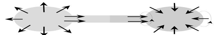
Figure 1: The topologically non-trivial field configuration is constructed from two oppositely charged monopoles, rotating one of them over a full $2\pi$ rotation.

In ${\rm I\kern-1.79993ptR}^{4}$ the topological charge is related to the winding of a gauge function $g(x)$ defined at infinity, which therefore is a mapping from $S^{3}$ to the gauge group. The way $g(x)$ enters is through requiring the Euclidean action,

$$S=-\frac{1}{2e^{2}}\int d^{4}x~{}{\rm Tr}\left(F^{2}_{\mu\nu}(x)\right),$$ (9)

to remain finite. As before this implies the field strength at infinity to go to zero, where $A_{\mu}(x)$ can be written as a pure gauge, $A_{\mu}(x)=g(x)\partial_{\mu}g^{-1}(x)$. For $SU(2)$ a simple parametrization as $g(x)=a_{\mu}(x)\sigma_{\mu}$ in terms of a unit vector $a_{\mu}$ and unit quaternions $\sigma_{\mu}=(\Eins_{2},i\vec{\tau})$ ($\bar{\sigma}_{\mu}\equiv\sigma_{\mu}^{\dagger}$) makes this winding most transparent as the mapping degree of $a(x)$ at infinity. In the simplest case of degree 1, $a(x)=x/|x|$ is a 4-dimensional hedgehog. The relation to Taubes’ construction is using the fact that $S^{3}$ can be viewed as a twisted product of $S^{1}$ (the Taubes winding) and $S^{2}$ (the hedgehog formed by the Higgs field), the so-called Hopf fibration [11, 16].

In the case of periodicity in the imaginary time direction as it occurs for calorons, let us transform $A_{0}(x)\to 0$ everywhere. This can be done by a time dependent gauge transformation $U(x)$, which in general will not be periodic. Actually $P(t;\vec{x})$ itself is the gauge transformation that relates the gauge field at $t+\beta$ to that at $t$ in the $A_{0}=0$ gauge. Since $P(x)$ goes to a constant (${{\cal P}_{\infty}}$) at spatial infinity, this provides a non-trivial mapping from $S^{3}$ (as ${\rm I\kern-1.79993ptR}^{3}$ compactified at infinity) to the gauge group. The topological charge is precisely its winding number.

As in the case of the monopole energy density, we can rewrite the action density in terms of a square and a boundary term,

$${\rm Tr}(F_{\mu\nu}^{2}) = {\scriptstyle{{1\over 2}}}{\rm Tr}(F_{\mu\nu}\pm\tilde{F}_{\mu\nu})^{2}\mp{\rm Tr}(F_{\mu\nu}\tilde{F}_{\mu\nu}),\quad{\rm Tr}(F_{\mu\nu}\tilde{F}_{\mu\nu})=\partial_{\mu}K_{\mu},$$

$$K_{\mu} = 2\varepsilon_{\mu\nu\alpha\beta}{\rm Tr}(A_{\nu}\partial_{\alpha}A_{\beta}+{\scriptstyle{{2\over 3}}}A_{\nu}A_{\alpha}A_{\beta}),$$ (10)

with $\tilde{F}_{\mu\nu}={\scriptstyle{{1\over 2}}}\varepsilon_{\mu\nu\alpha\beta}F_{\alpha\beta}$ the dual field strength interchanging electric and magnetic components. Hence, for self-dual solutions at finite temperature

$$S=\frac{1}{2e^{2}}\int\left(K_{0}(0,\vec{x})-K_{0}(\beta,\vec{x})\right)d^{3}x=\frac{1}{3e^{2}}\int{\rm Tr}(P(\vec{x})dP^{-1}(\vec{x}))^{3},$$ (11)

using that in the $A_{0}=0$ gauge $A(\beta,\vec{x})={}^{P}A(0,\vec{x})$, expressing the result in a compact differential form notation. Note that the integral is invariant under small deformations of $P$, using $\delta(PdP^{-1})^{3}=3d{\rm Tr}(P\delta P^{-1}(PdP^{-1})^{2})$, and therefore should be proportional to the winding number of $P$. A map of degree $k$ can be obtained by multiplying $k$ maps of degree 1 (the inverse gives a negative mapping degree). Each of these maps of degree 1 can be deformed at will, as the integral is invariant under continuous deformations, and in particular can be arranged to be the identity except for a small region. Choosing these regions to have no overlap, the integral is easily seen to be proportional to $k$. To fix for SU(2) the constant of proportionality we may take $U(\vec{x})=((1-|\vec{x}|^{2})\sigma_{0}+2\vec{x}\cdot\vec{\sigma})/(1+|\vec{x}|^{2})$, for the map of degree 1 related to stereographic projection from $S^{3}$ to ${\rm I\kern-1.79993ptR}^{3}$. For SU($n$) we first deform the map to lie in an SU(2) subgroup. This then gives the celebrated result that self-dual solutions with given topological charge, $k=(16\pi^{2})^{-1}\int d^{4}x{\rm Tr}\left(F_{\mu\nu}(x)\tilde{F}_{\mu\nu}(x)\right)$, have an action equal $8\pi^{2}|k|/e^{2}$.

This is also a convenient setting to understand why in the limit of zero temperature, $\beta\to\infty$, an instanton corresponds to vacuum to vacuum tunneling. Finite action requires the field strength to go to zero at $|t|\to\infty$, but at the same time, the field at $t\to\infty$ is related to the field at $t\to-\infty$ by a topologically non-trivial gauge transformation. Strictly speaking, we need to identify gauge field configuration that are gauge equivalent. Instead of having multiple vacua we can alternatively say there is one vacuum, with the field space being non-contractible. This is quite analogous to considering a periodic quantum mechanics problem, which could be reinterpreted as quantum mechanics on a circle. Tunneling now corresponds to penetration of the wave function in the classically forbidden region, to reach back to the vacuum going around the circle in either direction. Essential is that the support of the wave function, the region where it is non-vanishing, becomes sensitive to the non-trivial topology of the configuration space [3].

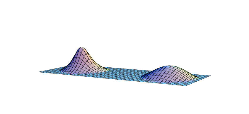
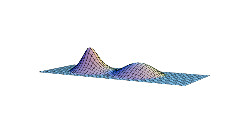
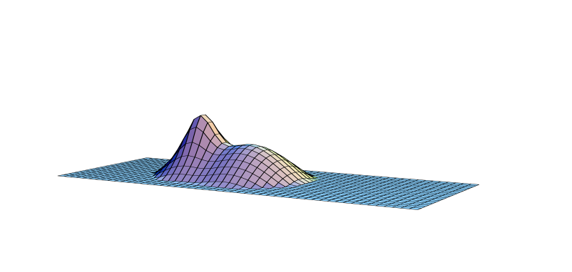
Figure 2: Shown is a typical example for the action density (on equal logarithmic scales at the time where it is maximal) of an SU(2) caloron with non-trivial holonomy $\mu_{2}=-\mu_{1}=0.125$ (for, from left to right, $\rho/\beta=0.8,1.2,1.6$).

The tunneling path in non-Abelian gauge theories is of course described by the one parameter ($t$) family of gauge fields $A_{i}(t,\vec{x})$ (in the $A_{0}=0$ gauge), and a finite action means we have to cross a potential barrier when going around the non-contractible loop (or going from vacuum to vacuum). From Taubes’ argument it is already clear that this intermediate configuration can be associated to a monopole-antimonopole boundstate, which is made more precise by the caloron solutions to be described. At zero-temperature this is less obvious, since there monopoles form close pairs, cmp. Fig. 2 (left). They behave very much like virtual particles, that can only be created for a short period of time, thereby explaining the instantaneous character. At finite temperature, the monopoles can be separated much more easily due to the interactions with the thermal bath. At high temperature, however, they will be suppressed due to the Boltzmann weight, and so monopoles (like calorons) are expected to be dilute. At low temperature instantons form a more dense ensemble, possibly leading to monopoles to be dense as well, particularly when instantons overlap. One may then have some hope that the confining electric phase could be characterized by a deconfining magnetic phase, where the dual deconfinement is due to the large monopole density, in a similar spirit to high density induced quark deconfinement. It would offer a possible alternative to existing scenarios.

Instantons describe virtual processes and are quite often discussed in the context of the semiclassical approximation. For a one-dimensional particle with mass $m$ in a positive potential $V$ we may again split off a square,

$$\hskip-14.22636ptL(t)\!=\!{\scriptstyle{{1\over 2}}}m\dot{x}^{2}(t)\!+\!V(x(t))\!=\!{\scriptstyle{{1\over 2}}}m\left(\dot{x}(t)-\sqrt{2V(x(t))/m}\right)^{2}\!\!+\dot{x}(t)\sqrt{2mV(x(t))},$$

$$\hskip-9.95845ptS_{cl}=\int dt~{}\dot{x}(t)\sqrt{2mV(x(t))}=\int dx\sqrt{2mV(x)},$$ (12)

where we typically integrate between the classical turning points, related to the WKB expression for the wave function in the classically forbidden region, $\exp(-\int_{x_{0}}^{x}dy\sqrt{2mV(y)}/\hbar)$. In a double well this leads to a tunnel splitting proportional to $\exp(-S_{cl}/\hbar)$. One problem in the theory of strong interactions is that the effective coupling tends to become too big for large instantons. Instantons can have an arbitrary size $\rho$, due to the classical scale invariance of the theory. This classical scale invariance gets broken by the regularization and one is left with a scale dependent running coupling constant after renormalization. This causes a problem when integrating over the scale parameter in the one-instanton tunneling amplitude given by the celebrated result of ’t Hooft [17], $dW\propto d\rho dx^{4}\rho^{-5}\exp\left(-8\pi^{2}/e^{2}(\rho)\right)$. Actually, for calorons with non-trivial holonomy and $\rho>\beta$, it is more natural to associate $\rho$ with the distance between constituent monopoles ($\pi\rho^{2}/\beta$ for SU(2)), and this may help alleviate the problem one encounters when dealing with large scale instantons. This is also one way to understand why there will still be calorons with $\rho$ arbitrary, despite the fact that $\beta$ fixes the scale. At zero temperature, a large $\rho$ leads to a low energy barrier along the tunneling path, and at some point this will no longer describe a virtual process and the semiclassical approximation will break down. Nevertheless, the instanton liquid model has been very successful in describing much of the low energy phenomenology, in particular for chiral dynamics and aspects related to breaking the axial U(1) symmetry. We refer to the reviews by Schäfer and Shuryak [20] and by Diakonov [21] for more details.

1.3 Fermion zero-modes

In the instanton liquid model the interaction of instantons with fermions plays an important role. This is because instantons have a remarkable influence on the spectrum of Dirac fermions, it namely implies the presence of zero eigenvalue solutions with fixed chirality (the so-called chiral zero-modes). These chiral zero-modes will play an important role in the Nahm transformation and in studying the properties of the calorons with non-trivial holonomy, so we wish to mention some of the interesting and far reaching physical consequences. This is most easily discussed in terms of the spectral flow of the Dirac Hamiltonian along the tunneling path. Its spectrum is of course gauge invariant, and this implies that the energy levels at $t=0$ and $t=\beta$ are identical. The gauge field provides a smooth interpolation between these, which leads to each of the energies to be a continuous function of $t$, the so-called spectral flow, see Fig 3.

$E=0$
             $E=-\Lambda$                       $t=0$                                                 $t=\beta$

Figure 3: Schematic representation of the spectral flow.

If we draw the energy level at zero, the number of crossings is clearly a conserved quantity, it cannot change under continuous deformations of the gauge field background (the background need not be a solution of the equations of motion). It is also clear, by putting instantons in a row, that the number of crossings is proportional to the topological charge, and not surprisingly it is actually equal to it. The necessity of such a crossing is related to the existence of a chiral zero-mode, whose number for fermions in the fundamental representation is equal to the topological charge, as follows from the Atiyah-Singer index theorem [22]. The argument is most simple in the case of zero-temperature, where the zero-mode at $t\to\pm\infty$ has to behave as $\exp(-tE_{\pm})$, where $E_{\pm}$ is one of (free) fermion energies. Clearly this would only give a normalizable zero-mode if $E_{+}>0$ and $E_{-}<0$, which forces a crossing! At this point the Dirac vacuum is degenerate and particles or anti-particles are created with definite chirality. Compatible with the breaking of the axial U(1) symmetry, the divergences of its current is proportional to the topological density $\tilde{F}_{\mu\nu}F_{\mu\nu}$. It gives rise to the so-called ’t Hooft interaction [17], which together with a finite density of fermion modes at zero eigenvalue (required for the Banks-Casher mechanism [23] to work) play an important role in the spontaneous breaking of chiral symmetry (or soft breaking in case of small up and down quark masses) [20]. Finally, the spectral flow also makes it easy to understand the origin of the axial anomaly, which occurs due to the need to regularize the theory. If cutting off modes with $E<-\Lambda$, where $\Lambda$ is the ultraviolet cutoff, we see that the spectral flow leads to the fact that modes we had removed in the trivial vacuum reappear due to the spectral flow at the vacuum equivalent to it by a topologically non-trivial gauge transformation. That the violation in conserving the axial U(1) charge is proportional to the topological charge is in this setting simply a consequence of the number of crossings in the spectral flow. This is the celebrated infrared-ultraviolet connection, and also makes it understandable why the anomaly is robust (fully determined by the lowest order result in perturbation theory).

2 Construction of solutions

Let us start with the well know SU(2) Harrington-Shepard solution [1] for the caloron with trivial holonomy. In that case one simply takes a periodic array of instantons parallel in group space (${{\cal P}_{\infty}}=\Eins_{2}$), placed at $a_{(p)}\equiv(a_{0}+p\beta,\vec{a})$ for integer $p$. The solution is found in terms of the ’t Hooft ansatz [24], which in its general form is given by

$$A_{\mu}(x)={\scriptstyle{{1\over 2}}}\bar{\eta}_{\mu\nu}\partial_{\nu}\log\phi(x).$$ (13)

Here $\eta_{\mu\nu}={\scriptstyle{{1\over 2}}}(\sigma_{\mu}\bar{\sigma}_{\nu}-\sigma_{\nu}\bar{\sigma}_{\mu})=i\eta_{\mu\nu}^{a}\tau_{a}$ and $\bar{\eta}_{\mu\nu}={\scriptstyle{{1\over 2}}}(\bar{\sigma}_{\mu}\sigma_{\nu}-\bar{\sigma}_{\nu}\sigma_{\mu})=i\bar{\eta}_{\mu\nu}^{a}\tau_{a}$, are the self-dual and anti-selfdual ’t Hooft tensors. Substituting this in the self-duality equation, $F_{\mu\nu}=\tilde{F}_{\mu\nu}$, one finds this is a solutions if and only if $\partial_{\mu}^{2}\phi(x)=0$. Therefore $\phi=1+\sum_{i=1}^{k}\rho_{i}^{2}|x-b_{(i)}|^{2}$, where $b_{(i)}$ are the four dimensional locations and $\rho_{i}$ the sizes of the $k$ instantons. A singularity at $x=b_{(i)}$ can be removed by a gauge transformation. For the Harrington-Shepard solution, taking $b_{(p)}=a_{(p)}$ and $\rho_{p}=\rho$ one can perform the sum over $p\in{\mathbb{Z}}$ to find [1],

$$\phi_{HS}(x)=1+\frac{\pi\rho^{2}\sinh(2\pi r/\beta)/(\beta r)}{\cosh(2\pi r/\beta)-\cos(2\pi(t-a_{0})/\beta)},\quad r=|\vec{x}-\vec{a}|.$$ (14)

The case of non-trivial holonomy cannot be treated in the same way, because we will have to sum over a periodic array of instantons that has a color rotation by ${{\cal P}_{\infty}}$ when shifting time over $\beta$. This can only be treated within the full ADHM ansatz. The rest of this section is more technical and could be skipped, although the short tutorials on the ADHM construction and the Nahm transformation in Secs. 2.1 and 2.2 are still recommended.

2.1 ADHM formalism

The $SU(n)$ ADHM construction for charge $k$ instantons [14] starts with a $k$ dimensional vector $\lambda=(\lambda_{1},\ldots,\lambda_{k})$, where $\lambda_{i}^{\dagger}$ is a two-component spinor in the $\bar{n}$ representation of $SU(n)$ (i.e. $\lambda$ is a $n\times 2k$ complex matrix) and a $2k\times 2k$ complex matrix $B=\sigma_{\mu}\otimes B_{\mu}$ (each $B_{\mu}$ is a hermitian $k\times k$ matrix). These are combined to form a $(n+2k)\times 2k$ dimensional matrix $\Delta(x)$, which has $n$ normalized eigenvectors with vanishing eigenvalue, combined in a complex matrix $v(x)$ of size $(n+2k)\times n$,

$$\Delta(x)=\left(\!\!\begin{array}[]{c}\lambda\\ B(x)\end{array}\!\!\right),\quad B(x)=B-x\Eins_{k},\quad\Delta^{\dagger}(x)v(x)=0.$$ (15)

Here the quaternion $x=x_{\mu}\sigma_{\mu}$ (a $2\times 2$ matrix with spinor indices) denotes the position and $v(x)$ can be solved explicitly in terms of the ADHM data,

$$v(x)\!=\!\!\left(\!\!\begin{array}[]{c}-{\Eins}_{n}\\ u(x)\end{array}\!\!\right)\phi^{-{\scriptstyle{{1/2}}}}\!,\quad u(x)\!=\!(B^{\dagger}\!-\!x^{\dagger})^{-1}\lambda^{\dagger},\quad\phi(x)\!=\!{\Eins}_{n}\!+\!u^{\dagger}(x)u(x).$$ (16)

The square root $\phi^{{\scriptstyle{{1/2}}}}(x)$ is well-defined because $\phi(x)$ is a positive $n\times n$ hermitian matrix. The gauge field is now given by

$$A(x)\equiv A_{\mu}(x)dx_{\mu}=v^{\dagger}(x)dv(x)$$ (17)

and to check its self-duality it is best to use form notation. For the field strength two form $F(x)={\scriptstyle{{1\over 2}}}F_{\mu\nu}(x)dx_{\mu}\wedge dx_{\nu}=dA(x)+A(x)\wedge A(x)$ we find

$$F=d(v^{\dagger}dv)+v^{\dagger}dv\wedge v^{\dagger}dv=dv^{\dagger}\wedge(1-v\otimes v^{\dagger})dv.$$ (18)

We note that $v\otimes v^{\dagger}$ projects to the kernel of $\Delta^{\dagger}$. Assuming that $\Delta$ has no zero eigenvalues such that $\Delta^{\dagger}\Delta$ is invertible, we find that $1-v\otimes v^{\dagger}=\Delta(\Delta^{\dagger}\Delta)^{-1}\Delta^{\dagger}$. Indeed, when acting on elements in the kernel of $\Delta^{\dagger}$, left- and right-hand side are equal. Any vector in the orthogonal complement of this kernel can be written as $\Delta w$, since $<v,\Delta w>=<\Delta^{\dagger}v,w>=0$, such that left- and right-hand side are again equal. Hence

$$F=dv^{\dagger}\Delta\wedge(\Delta^{\dagger}\Delta)^{-1}\Delta^{\dagger}dv=dv^{\dagger}bdx\wedge(\Delta^{\dagger}\Delta)^{-1}dx^{\dagger}b^{\dagger}dv,$$ (19)

where we use the fact that $\Delta^{\dagger}dv=(d\Delta^{\dagger})v=dx^{\dagger}b^{\dagger}v$, with $b^{\dagger}=(0~{}\Eins_{2}\otimes\Eins_{k})$ as a $2k\times(n+2k)$ matrix. It might seem this does not help that much, but remarkably, using $dx=dx_{\mu}\sigma_{\mu}$ we find $dx\wedge dx^{\dagger}=\eta_{\mu\nu}dx_{\mu}\wedge dx_{\nu}$, and since $\eta_{\mu\nu}$ is self-dual, we are done. Not quite so yet! We had to take $dx\otimes\Eins_{k}$ through $(\Delta^{\dagger}\Delta)^{-1}$ and this is only possible if

$$(\Delta^{\dagger}(x)\Delta(x))^{-1}=\Eins_{2}\otimes f_{x},$$ (20)

where $f_{x}$ is a hermitian $k\times k$ matrix. This condition, stating that $\Delta^{\dagger}(x)\Delta(x)$ is invertible and commutes with the quaternions, is what is known as the quadratic ADHM constraint. It has reduced solving a set of non-linear partial differential equations to solving a quadratic matrix equation.

To construct a charge $k$ caloron with non-trivial holonomy [26], we place $k$ instantons in the time interval $[0,\beta[$, performing a color rotation with ${{\cal P}_{\infty}}$ for each shift of $t$ over $\beta$, cmp. Eq. (3). This is implemented by requiring (suppressing color and spinor indices and scaling $\beta$ to 1 in this section)

$$\lambda_{pk+k+a}={{\cal P}_{\infty}}\lambda_{pk+a},\quad B_{pk+a,qk+b}=B_{pk-k+a,qk-k+b}+\sigma_{0}\delta_{pq}\delta_{ab}.$$ (21)

Solutions to these equations are parametrized by $\zeta_{a}$ and $\hat{A}^{ab}_{p}$,

$$\lambda_{pk+a}={\cal{P}}^{p}_{\infty}\zeta_{a},\quad B_{pk+a,qk+b}=p\sigma_{0}\delta_{pq}\delta_{ab}+\hat{A}^{ab}_{p-q},$$ (22)

with $\hat{A}$ to be determined by the quadratic ADHM constraint.

2.2 Fourier-Nahm transformation

We introduce the $n$ projectors $P_{m}$ on the $m$th eigenvalue of ${{\cal P}_{\infty}}$, such that ${{\cal P}_{\infty}}=\sum_{m}e^{2\pi i\mu_{m}}P_{m}$ and $\lambda_{pk+a}=\sum_{m}e^{2\pi ip\mu_{m}}P_{m}\zeta_{a}$. Fourier transformation now leads to

$$2\pi i\sum_{p}e^{2\pi ipz}\hat{A}^{ab}_{p}=\hat{A}^{ab}(z),\quad\sum_{p}e^{-2\pi ipz}\lambda_{pk+a}=\sum_{m}\delta(z-\mu_{m})P_{m}\zeta_{a}.$$ (23)

Here $\zeta_{a}^{\dagger}$ is again a two-component spinor in the $\bar{n}$ representation of $SU(n)$ and $\hat{A}^{ab}(z)=\sigma^{\mu}\hat{A}^{ab}_{\mu}(z)$, with $\hat{A}_{\mu}(z)$ an anti-hermitian $k\times k$ matrix. In terms of the latter

$$\sum_{p,q}B_{pk+a,qk+b}(x)e^{2\pi i(pz-qz^{\prime})}=\frac{\delta(z-z^{\prime})}{2\pi i}\hat{D}_{x}^{ab}(z^{\prime}),$$ (24)

$$\hat{D}_{x}^{ab}(z)\equiv\hat{D}^{ab}(z)-2\pi ix\delta^{ab}=\sigma_{0}\delta^{ab}{\frac{d}{dz}}+\hat{A}^{ab}(z)-2\pi ix\delta^{ab},$$

which is the Weyl operator (positive chirality Dirac operator) for the U($k$) gauge field $\hat{A}_{\mu}(z)\!-\!2\pi ix_{\mu}\Eins_{k}$ defined on the circle, $z\!\in\![0,1]$, i.e. with periodicity 1 ($\beta^{-1}$ in case $\beta\neq 1$). The quadratic ADHM constraint now reads

$$\Bigl{[}\sigma_{i}\otimes\Eins_{k},D_{x}^{\dagger}(z)D_{x}(z)+4\pi^{2}\sum_{m}\delta(z-\mu_{m})\zeta_{a}^{\dagger}P_{m}\zeta_{b}\Bigr{]}=0.$$ (25)

Introducing

$$2\pi\zeta_{a}^{\dagger}P_{m}\zeta_{b}\equiv\Eins_{2}\hat{S}_{m}^{ab}-\vec{\tau}\cdot\vec{\rho}_{m}^{\,ab},$$ (26)

this leads precisely to the so-called Nahm equation [13],

$${\frac{d}{dz}}\hat{A}_{j}(z)+[\hat{A}_{0}(z),\hat{A}_{j}(z)]+{\scriptstyle{{1\over 2}}}\varepsilon_{jk\ell}[\hat{A}_{k}(z),\hat{A}_{\ell}(z)]=2\pi i\sum_{m}\delta(z-\mu_{m})\rho_{m}^{\,j}.$$ (27)

Note that the left-hand side is the difference between the magnetic and electric field for $\hat{A}_{\mu}(z)$, with the right-hand side a violation of self-duality.

Although we do not want to go into too much detail here, it is instructive to discuss the standard setting of the Nahm transformation [13, 27]. One starts from an SU($n$), charge $k$ self-dual gauge field on ${\rm I\kern-1.79993ptR}^{4}$ with periods in all four directions, some of which may be infinite or zero (in the latter case effectively leading to a reduced dimension). This extends to a family of self-dual U($n$) gauge fields when adding $-2\pi iz_{\mu}\Eins_{n}$ to the SU($n$) gauge field $A_{\mu}(x)$. The index theorem now guarantees there is a family of $k$ chiral zero-modes for the Weyl equation $D_{z}^{\dagger}\Psi(x;z)=-\bar{\sigma}_{\mu}D_{\mu}(x;z)\Psi(x;z)=0$, and this allows one to construct the gauge field $\hat{A}^{ab}_{\mu}(z)=\int d^{4}x\Psi^{a}(x;z)^{\dagger}\partial\Psi^{b}(x;z)/\partial z_{\mu}$. This dual U($k$) gauge field can be shown to be self-dual with charge $n$, and is defined again on ${\rm I\kern-1.79993ptR}^{4}$, but with its periods inverted. Remarkably, one can then perform the transformation again, and come back to the original gauge field [27].

The ADHM construction performs precisely this last step. For instantons on ${\rm I\kern-1.79993ptR}^{4}$ all periods are infinite and the Nahm transformation reduces self-duality to algebraic equations. Singularities may appear (except when all periods are finite), as we have seen from our analysis using Fourier transformation of the ADHM data and like in ${\rm I\kern-1.79993ptR}^{4}$ are related to introducing $\lambda$, which encodes the asymptotic behavior of the zero-modes.

One final result is crucial to appreciate the strength of this formalism,

$$D^{\dagger}_{z}D_{z}=-\Eins_{2}\otimes D^{2}_{\mu}(x;z)-\bar{\eta}_{\mu\nu}\otimes[D_{\mu}(x;z),D_{\nu}(x;z)],$$ (28)

which uses the fact that $\bar{\sigma}_{\mu}\sigma_{\nu}=\delta_{\mu\nu}\Eins_{2}+\bar{\eta}_{\mu\nu}$. Since $[D_{\mu}(x;z),D_{\nu}(x;z)]=F_{\mu\nu}(x)$ and the contraction of an anti-self dual tensor ($\bar{\eta}_{\mu\nu}$) with a self-dual tensor ($F_{\mu\nu}$) vanishes, self-duality implies that $D^{\dagger}_{z}D_{z}=-\Eins_{2}\otimes D^{2}_{\mu}(x;z)$, which therefore commutes with the quarternions. This is completely analogous to our discussion for the ADHM construction, and proves that the Nahm gauge field $\hat{A}_{\mu}(z)$ is self-dual. Doing the Nahm transformation for the second time leads us to perform the same calculation as in Eq. (28), this time for the dual Weyl operator $\hat{D}_{x}$, and we see that the quadratic ADHM constraint is fully equivalent with stating that the dual gauge field is self-dual. The only complication is the possible presence of singularities when some of the periods are infinite, in particular for the ADHM construction somewhat hiding this profound relationship to the Nahm transformation.

2.3 Some explicit formulae

One might think all of this is just pushing the same problem around, but as we noted before, there is a dramatic simplification due to the dimensional reduction. In addition, for topological charge 1 the dual gauge field is Abelian, further simplifying the Nahm equation. In that case all the commutator terms in Eq. (27) vanish, and $\hat{A}_{\mu}(z)$ is piecewise constant, only jumping at the singularities. It is this that has allowed us to make progress in finding explicit solutions, together with the “magic” formulae for gauge field, action density, fermion zero-modes and density found previously within the ADHM formalism [28, 29],

$$A_{\mu}(x)={\scriptstyle{{1\over 2}}}\phi^{\scriptstyle{{1/2}}}(x)\bar{\eta}_{\mu\nu}^{j}\partial_{\nu}\phi_{j}(x)\phi^{\scriptstyle{{1/2}}}(x)+{\scriptstyle{{1\over 2}}}[\phi^{-{\scriptstyle{{1/2}}}}(x),\partial_{\mu}\phi^{\scriptstyle{{1/2}}}(x)],$$ (29)

$$\hskip-14.22636pt\Psi_{iI}^{l}(x)\!=\!(2\pi)^{-1}\left(\phi^{\scriptstyle{{1/2}}}(x)\lambda\partial_{\mu}f_{x}\bar{\sigma}_{\mu}\varepsilon\right)_{iI}^{l},\quad\Psi^{l}_{iI}(x)^{*}\Psi^{m}_{iI}(x)\!=\!-(2\pi)^{-2}\partial_{\mu}^{2}f^{lm}_{x},$$

where $l=1,\ldots,k$ labels the zero-modes ($i,I$ are the gauge and spin index),

$$\phi(x)=\left({\Eins}_{n}-\phi_{0}\right)^{-1},\quad\phi_{\mu}\equiv\lambda(\sigma_{\mu}\!\otimes\!f_{x})\lambda^{\dagger},\quad\varepsilon\equiv\sigma_{2}=i\tau_{2}.$$ (30)

The gauge field for SU(2) further simplifies to $A_{\mu}(x)={\scriptstyle{{1\over 2}}}\phi(x)\bar{\eta}_{\mu\nu}^{j}\partial_{\nu}\phi_{j}(x)$ (which could be viewed as a generalized ’t Hooft ansatz), since in that case $\phi(x)$ as a $2\times 2$ matrix is a multiple of $\Eins_{2}$. For the action density one finds [29],

$${\rm Tr}F_{\mu\nu}^{2}(x)=-\partial^{2}_{\mu}\partial^{2}_{\nu}\log\det f_{x}.$$ (31)

It is thus very convenient to first find the matrix $f_{x}$, as defined in Eq. (20). For calorons, after Fourier transformation, it is replaced by the Green’s function $\hat{f}_{x}(z,z^{\prime})$, which satisfies the equation [26]

$$\left\{\left(\frac{\hat{D}_{\mu}(z;x)}{2\pi i}\right)^{\!\!2}\!+\frac{1}{2\pi}\sum_{m}\delta(z\!-\!\mu_{m})\hat{S}_{m}\right\}\!\hat{f}_{x}(z,z^{\prime})={\Eins}_{k}\delta(z\!-\!z^{\prime}).$$ (32)

The gauge field, as determined through $\phi_{\mu}(x)$, see Eq. (29), is read off from

$$\phi_{\mu}(x)=\sum_{m,m^{\prime}}P_{m}\zeta_{a}\sigma_{\mu}\hat{f}_{x}^{ab}(\mu_{m},\mu_{m^{\prime}})\zeta^{\dagger}_{b}P_{m^{\prime}},$$ (33)

whereas the fermion zero-modes satisfying a generalized boundary condition $\hat{\Psi}_{z}^{a}(t+1,\vec{x})=e^{2\pi iz}{{\cal P}_{\infty}}\hat{\Psi}_{z}^{a}(t,\vec{x})$, cmp. Eq. (3), are given by [30, 31]

$$\hat{\Psi}_{z}^{a}(x)=(2\pi)^{-1}\phi^{\scriptstyle{{1/2}}}(x)\sum_{m}P_{m}\zeta_{b}\bar{\sigma}_{\mu}\varepsilon\partial_{\mu}\hat{f}^{ba}_{x}(\mu_{m},z).$$ (34)

For $z={\scriptstyle{{1\over 2}}}$ this gives the usual anti-periodic boundary conditions for fermions at finite temperature, but the general $z$ dependence will turn out to be extremely useful as a diagnostic tool. Finally, the zero-mode density reads

$$\hat{\Psi}_{z}^{a}(x)^{\dagger}\hat{\Psi}_{z}^{b}(x)=-(2\pi)^{-2}\partial_{\mu}^{2}\hat{f}^{ab}_{x}(z,z).$$ (35)

To compute $\hat{f}_{x}(z,z^{\prime})$ we note that we can always transform to a gauge where $\hat{A}_{0}(z)\equiv 2\pi i\xi_{0}$ is constant, after which $\hat{g}(z)\equiv\exp(2\pi i(\xi_{0}-x_{0}\Eins_{k})z)$ transforms $\hat{A}_{0}(z)-2\pi ix_{0}$ to zero. This turns Eq. (32) into

$$\left\{-\frac{d^{2}}{dz^{2}}+V(z;\vec{x})\right\}\!f_{x}(z,z^{\prime})=4\pi^{2}{\Eins}_{k}\delta(z\!-\!z^{\prime}),$$ (36)

with $f_{x}(z,z^{\prime})$ and $V(z;\vec{x})$ given by

$$\hskip-11.38109ptf_{x}(z,z^{\prime})\!\equiv\!\hat{g}(z)\hat{f}_{x}(z,z^{\prime})\hat{g}^{\dagger}(z^{\prime}),\quad V(z;\vec{x})\!\equiv\!4\pi^{2}\vec{R}^{2}(z;\vec{x})\!+\!2\pi\!\!\sum_{m}\delta(z\!-\!\mu_{m})S_{m},$$

$$\hskip-11.38109ptR_{j}(z;\vec{x})\equiv x_{j}{\Eins}_{k}-(2\pi i)^{-1}\hat{g}(z)\hat{A}_{j}(z)\hat{g}^{\dagger}(z),\quad S_{m}\equiv\hat{g}(\mu_{m})\hat{S}_{m}\hat{g}^{\dagger}(\mu_{m}).$$ (37)

Periodicity is now only up to the gauge transformation $\hat{g}(1)$. In particular when $\vec{R}^{\,2}(z;\vec{x})$ is piecewise constant explicitly computing the Green’s function becomes doable. Nevertheless, in general terms one finds

$$\hskip-11.38109ptf_{x}(z,z^{\prime})=4\pi^{2}\left\{W(z,z_{0})\left(\theta(z^{\prime}-z){\Eins}_{2k}-({\Eins}_{2k}-{\cal{F}}_{z_{0}})^{-1}\right)W^{-1}(z^{\prime},z_{0})\right\}_{12},$$

$$\hskip-11.38109ptW(z_{2},z_{1})\equiv{\rm Pexp}\int_{z_{1}}^{z_{2}}\pmatrix{0&{\Eins}_{k}\cr V(z;\vec{x})&0\cr}dz,\quad{\cal{F}}_{z_{0}}\equiv\hat{g}^{\dagger}(1)W(z_{0}\!+\!1,z_{0}).$$ (38)

where the $(1,2)$ component on the right-hand side for $f_{x}(z,z^{\prime})$ is with respect to the $2\times 2$ block matrix structure. This equation for $f_{x}(z,z^{\prime})$ is valid for $z^{\prime}\in[z,z+1]$, but can be extended with the appropriate periodicity. We can now also find an explicit result for the action density

$$\quad{\rm Tr}F_{\mu\nu}^{2}(x)=\partial_{\mu}^{2}\partial_{\nu}^{2}\log\psi(x),\quad\psi(x)\equiv\det\left(ie^{-\pi ix_{0}}(\Eins_{2k}-{\cal{F}}_{z_{0}})/\sqrt{2}\right).$$ (39)

Note that $z_{0}$ can be chosen at will, e.g. for $z_{0}=\mu_{m}\!+0$ we find

$${\cal{F}}_{\mu_{m}}=T_{m}H_{m-1}\cdots T_{2}H_{1}T_{1}\hat{g}^{\dagger}(1)H_{n}T_{n}H_{n-1}\cdots T_{m+1}H_{m},$$ (40)

$$T_{m}\equiv\pmatrix{{\Eins}_{k}&0\cr 2\pi S_{m}&{\Eins}_{k}\cr},\quad H_{m}\equiv{\rm Pexp}\int_{\mu_{m}}^{\mu_{m+1}}\pmatrix{0&{\Eins}_{k}\cr 4\pi^{2}\vec{R}^{2}(z;\vec{x})&0\cr}dz.$$

The main pay off to have these expressions in terms of possibly unknown solutions to the Nahm equations, is that it allows us to look at the far field limit. When constituent monopoles are well separated, the charged components of the field in the core decay exponentially, being left with the Abelian fields in the far field region. This is related to the high temperature limit, in which case the cores collapse to zero size.

2.4 Limits and special cases

To extract exponential factors it turned out to be convenient to define

$$f_{m}^{\pm}(z)\!={\rm Pexp}\left[\pm 2\pi\!\int_{\mu_{m}}^{z}\!\!\!\!R_{m}^{\pm}(z)dz\right],\quad R_{m}^{\pm}(z)^{2}\pm\frac{1}{2\pi}{\frac{d}{dz}}\,R_{m}^{\pm}(z)\!=\!\vec{R}^{\,2}(z;\vec{x}).$$ (41)

Since $\vec{R}(z;\vec{x})\to\vec{x}{\Eins}_{k}$ for $|\vec{x}|\to\infty$, we find in this limit that $R_{m}^{\pm}(z)\to|\vec{x}|{\Eins}_{k}$ and $f_{m}^{\pm}(z)\to\exp\left(\pm 2\pi|\vec{x}|(z-\mu_{m}){\Eins}_{k}\right)$. For $z,z^{\prime}\in[\mu_{m},\mu_{m+1}]$ we can now write $W(z,z^{\prime})=W_{m}(z)W_{m}^{-1}(z^{\prime})$, see Eq. (38), with

$$W_{m}(z)\equiv\pmatrix{f_{m}^{+}(z)&f_{m}^{-}(z)\cr 2\pi R^{+}_{m}(z)f_{m}^{+}(z)&-2\pi R^{-}_{m}(z)f_{m}^{-}(z)\cr}.$$ (42)

This has allowed us to show that (ff stands for far field limit)

$$f^{\rm{ff}}_{x}(\mu_{m},\mu_{m})=2\pi\Sigma_{m}^{-1},~{}\mbox{and}~{}f^{\rm{ff}}_{x}(z,z)=\pi R_{m}^{-1}(z)\mbox{~{}for~{}}\mu_{m}\!<\!z\!<\!\mu_{m+1},$$ (43)

where $\Sigma_{m}\equiv R_{m}^{-}(\mu_{m})+R_{m-1}^{+}(\mu_{m})+S_{m}$ and $R_{m}(z)\equiv{\scriptstyle{{1\over 2}}}(R_{m}^{+}(z)+R_{m}^{-}(z))$. For this to hold $\vec{x}$ has to be far removed from any constituent. In addition $f^{\rm{ff}}(\mu_{m},\mu_{m+1})=0$, which implies that for SU(2) and SU(3) only the Abelian components of the gauge field survive in this limit.

Useful is also the so-called zero-mode limit (zm), which assumes $\vec{x}$ to be far removed from any constituent monopole other than of type $m$, distinguished by their magnetic charge and mass $8\pi^{2}\nu_{m}$, with $\nu_{m}\equiv\mu_{m+1}-\mu_{m}$, see the next section. In this limit one finds up to exponential corrections [31] for $\mu_{m}\leq z^{\prime}\leq z\leq\mu_{m+1}$ ($f_{x}(z^{\prime},z)=f_{x}^{\dagger}(z,z^{\prime})$ for $z^{\prime}>z$)

$$\hskip-11.38109ptf^{\rm{zm}}_{x}(z,z^{\prime})=\pi\left(f_{m}^{-}(z)f_{m}^{-}(\mu_{m+1})^{-1}\!-f_{m}^{+}(z)f_{m}^{+}(\mu_{m+1})^{-1}Z_{m+1}^{-}\right)\times$$ (44)

$$\hskip-11.38109pt\left(f_{m}^{-}(\mu_{m+1})^{-1}\!-\!Z_{m}^{+}f_{m}^{+}(\mu_{m+1})^{-1}Z_{m+1}^{-}\right)^{-1}\!\!\left(f_{m}^{-}(z^{\prime})^{-1}\!-\!Z_{m}^{+}f_{m}^{+}(z^{\prime})^{-1}\right)R_{m}^{-1}(z^{\prime}),$$

with $Z_{m}^{-}\equiv{\Eins}_{k}-2\Sigma_{m}^{-1}R_{m-1}(\mu_{m})$ and $Z_{m}^{+}\equiv{\Eins}_{k}-2\Sigma_{m}^{-1}R_{m}(\mu_{m})$. One concludes that the zero-modes (see Eq. (34) and Eq. (35)) are localized exponentially to the $m$th constituent monopoles (for $z$ away from the interval boundaries).

$y$
                                                                                  $\xi$

Figure 4: Constituent locations $y$ based on Eq. (45) as a function of $\xi=\xi_{1}=-\xi_{2}$ for $y_{2}=-y_{1}=\nu_{1}=\nu_{2}={\scriptstyle{{1\over 2}}}$ and $\rho_{1}=\rho_{2}=2$. Dashed versus full lines distinguish the magnetic charge of the constituents. The dotted lines apply to Figs. 3.

Explicit solutions are found when $\vec{R}(z;\vec{x})\equiv\vec{x}-\vec{Y}(z)$ is piecewise constant, i.e. $\vec{Y}(z)\equiv\vec{Y}_{m}$ for $z\in[\mu_{m},\mu_{m+1}]$, in which case $|\vec{R}|=R_{m}^{\pm}=R_{m}$. Apart from $k=1$, this is so for a class of axially symmetric multi-caloron solutions [26], in which case $3k$ eigenvalues of $\vec{Y}_{m}$ give the locations of the type $m$ constituent monopoles. The expression for the zero-mode in that case can be used to show that in the high temperature limit the zero-mode densities reduce to delta functions localized at these constituent locations, thus establishing that the constituents in this limit are point-like monopoles. Particularly simple axially symmetric solutions are found for SU(2),

$$\zeta^{a}_{iI}=\rho_{a}\delta_{iI},\quad\vec{Y}^{ab}_{m}=\vec{e}(\delta_{ab}\xi_{a}+y_{m}\rho_{a}\rho_{b}),\quad\nu_{1}y_{1}+\nu_{2}y_{2}=0,\quad\rho_{a}>0.$$ (45)

For charge 2, choosing $\rho_{1}=\rho_{2}=2$ and equal mass constituents ($\nu_{1}=\nu_{2}={\scriptstyle{{1\over 2}}}$) the constituent locations $y$ are plotted as a function of $\xi=\xi_{1}=-\xi_{2}$ in Fig. 4. We note that opposite charges are found to alternate. The properties of these solutions will be further discussed in the next section.

More generally, for SU(2) and charge 2 we may borrow from the study of monopoles [13, 32] the general solution of the Nahm equations for $z\!\in\![\mu_{1},\mu_{2}]$

$$\hat{A}_{j}(z)\equiv 2\pi i\hat{g}^{\dagger}(z)h^{\dagger}\Bigl{(}a_{j}{\Eins}_{2}+{\cal{D}}{\cal{R}}_{jb}f_{b}(4\pi{\cal{D}}z)\tau_{b}\Bigr{)}h\hat{g}(z),$$ (46)

where $f_{j}(z)$ are the Jacobi elliptic functions

$$f_{1}(z)=\frac{{\bf k}^{\prime}}{cn_{\bf k}(z)},\quad f_{2}(z)=\frac{{\bf k}^{\prime}sn_{\bf k}(z)}{cn_{\bf k}(z)},\quad f_{3}(z)=\frac{dn_{\bf k}(z)}{cn_{\bf k}(z)}.$$ (47)

Here $\vec{a}$ is the center of mass for monopoles of a given type, ${\cal{R}}$ and $h$ are arbitrary spatial and gauge rotations, ${\cal{D}}$ is a scale parameter, and $0\leq{\bf k}\leq 1$ (${\bf k}^{\prime}\equiv\sqrt{1-{\bf k}^{2}}$) playing the role of a shape parameter, as will be discussed in the next section. In general all these parameters differ on the second interval where in addition $z$ is shifted to $z-{\scriptstyle{{1\over 2}}}$, but they are to be related through the discontinuities in the Nahm equation, Eq. (27). This tends to be rather restrictive, and is the point where the construction for calorons deviates from that for static monopoles.

Quite remarkably, although $\vec{R}(z;\vec{x})$ is no longer piecewise constant, the function ${\rm Tr}R^{-1}_{m}(z)$ is independent of $z\in[\mu_{m},\mu_{m+1}]$. This is a highly non-trivial consequence of the Nahm equations (from the point of view of integrability, it gives a constant of motion). The physical significance here is that it is directly related to the zero-mode density (summed over the zero-modes) in the high temperature limit, see Eq. (35) and Eq. (43),

$$\Bigl{(}\sum_{a}\hat{\Psi}_{z}^{a}(x)^{\dagger}\hat{\Psi}_{z}^{a}(x)\Bigr{)}^{\rm{ff}}=-\partial_{i}^{2}{\cal{V}}_{m}(\vec{x}),\quad{\cal{V}}_{m}(\vec{x})\equiv(4\pi)^{-1}{\rm Tr}R^{-1}_{m}(z).$$ (48)

Miraculously we have been able to calculate ${\cal{V}}_{m}(\vec{x})$ exactly [31], from which we will be able to draw conclusions on the pointlike nature of the constituents.

3 Properties of solutions

We start our tour of SU($n$) caloron solutions with those of charge 1. In this case the action density has a particularly simple form [33]

$$-{\scriptstyle{{1\over 2}}}{\rm Tr}F_{\mu\nu}^{\,2}(x)=-{\scriptstyle{{1\over 2}}}\partial_{\mu}^{2}\partial_{\nu}^{2}\log\psi(x),\quad\psi(x)={\scriptstyle{{1\over 2}}}{\rm tr}({\cal{A}}_{n}\cdots{\cal{A}}_{1})-\cos(2\pi t/\beta),$$

$${\cal{A}}_{m}\equiv\frac{1}{r_{m}}\left(\!\!\!\begin{array}[]{cc}r_{m}\!\!&|\vec{\rho}_{m+1}|\\ 0\!\!&r_{m+1}\end{array}\!\!\!\right)\left(\!\!\!\begin{array}[]{cc}\cosh(2\pi\nu_{m}r_{m}/\beta)\!\!&\sinh(2\pi\nu_{m}r_{m}/\beta)\\ \sinh(2\pi\nu_{m}r_{m}/\beta)\!\!&\cosh(2\pi\nu_{m}r_{m}/\beta)\end{array}\!\!\!\right).$$ (53)

Here $\nu_{m}=\mu_{m+1}-\mu_{m}$, $r_{m}=|\vec{r}_{m}|$, $\vec{r}_{m}=\vec{x}-\vec{y}_{m}$ and $\vec{\rho}_{m}=\vec{y}_{m}-\vec{y}_{m-1}$, where $\vec{y}_{m}$ ($\vec{y}_{n+m}\equiv\vec{y}_{m}$) are the constituent locations. A few typical examples for SU(2), where $|\vec{\rho}_{1}|=\pi\rho^{2}/\beta$ in terms of the instanton scale parameter $\rho$, are shown in Fig. 2 and for SU(3) in Fig. 5 (we apologize for a somewhat awkward choice of conventions in naming the vectors $\vec{\rho}_{m}$ and scale parameters $\rho_{a}=|\zeta_{a}|$). From this it is already clear that there are $n$ lumps, centered at $\vec{y}_{m}$ and that when well-separated they are static and spherically symmetric. The self-duality then guarantees each lump is a basic BPS monopole, which can be seen to contribute $8\pi^{2}\nu_{m}$ to the action, correctly summing to a total action $8\pi^{2}$. Interesting properties on the geometry of the moduli space and alternative approaches can be found in Refs. [34, 35, 36].

It is instructive to provide further evidence for the monopole nature of these constituent lumps. For this we take the far field limit (ff) of Eq. (53). In this limit $\vec{x}$ is assumed to be far from all constituent locations $\vec{y}_{m}$ and we find

$$\psi^{\rm{ff}}(x)={\scriptstyle{{1\over 2}}}\prod_{m=1}^{n}\frac{\left(r_{m}+r_{m+1}+|\vec{\rho}_{m+1}|\right)}{2r_{m}}e^{2\pi\nu_{m}r_{m}/\beta}.$$ (54)

Note that there is no longer any time dependence and the far field limit is equivalent to the high temperature limit $\beta\to 0$, where the monopole mass becomes infinite and the non-Abelian core collapses to zero size (the range of the exponentially decaying charged fields shrinks to zero). As we will argue, using $A_{\mu}^{\rm D}(\vec{x})$ as the gauge field for the basic self-dual Abelian Dirac monopole, one finds in a suitable gauge for the Abelian far field embedded in SU($n$), $A^{ab}_{\mu}(\vec{x})=\delta_{ab}\tilde{A}_{\mu}^{a}(\vec{x})$, with $\tilde{A}_{\mu}^{m}(\vec{x})={\scriptstyle{{1\over 2}}}A_{\mu}^{\rm D}(\vec{r}_{m})-{\scriptstyle{{1\over 2}}}A_{\mu}^{\rm D}(\vec{r}_{m-1})$, where $\vec{E}^{\rm D}(\vec{x})=\vec{B}^{\rm D}(\vec{x})=\vec{x}|\vec{x}|^{-3}$ are electric and magnetic fields of this self-dual Dirac monopole. One verifies that indeed $-{\scriptstyle{{1\over 2}}}{\rm Tr}F_{\mu\nu}^{\,2}(x)=-{\scriptstyle{{1\over 2}}}\partial_{i}^{2}\partial_{j}^{2}\log\psi^{\rm{ff}}(x)$ when substituting this gauge field.

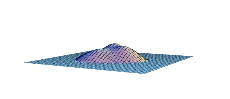
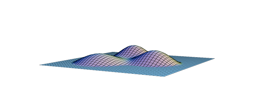
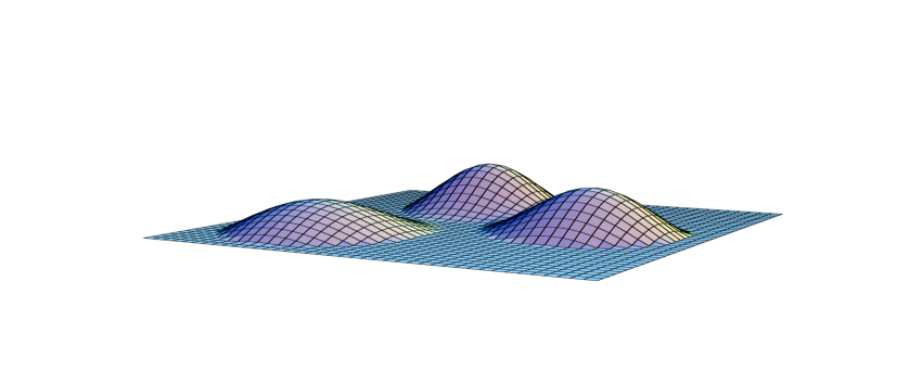
Figure 5: Action densities for the $SU(3)$ caloron with $(\mu_{1},\mu_{2},\mu_{3})=(-17,-2,19)/60$ and $(\nu_{1},\nu_{2},\nu_{3})=(0.25,0.35,0.4)$ at $t=0$ in the plane of the three constituents for $1/\beta=1.5$, 3 and 4 (from left to right) on equal logarithmic scales.

To give a little more insight in why the gauge field takes the above form, we remark that another way to define the location of an SU(2) monopole is to find the zeros of the Higgs field, or for SU($n$) to find where two of its eigenvalues coincide. At these points the broken gauge symmetry is partially restored to include an unbroken SU(2) subgroup. In the case of the caloron we of course need to find coinciding eigenvalues of the Polyakov loop, $P(\vec{x})$ [37]. The gauge field $\tilde{A}^{m}(\vec{x})$ defined above is associated to the Abelian component of the embedded SU(2) monopole associated to the unbroken subgroup. The Polyakov loop therefore is a useful diagnostic tool particularly when monopoles are too close to be seen as separate lumps. For SU(2) the constituents are simply found where $P(\vec{x})=\pm\Eins_{2}$ [38].

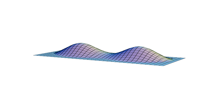
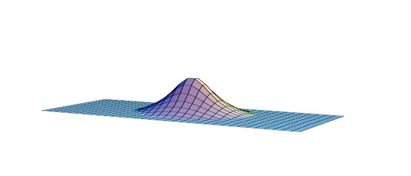
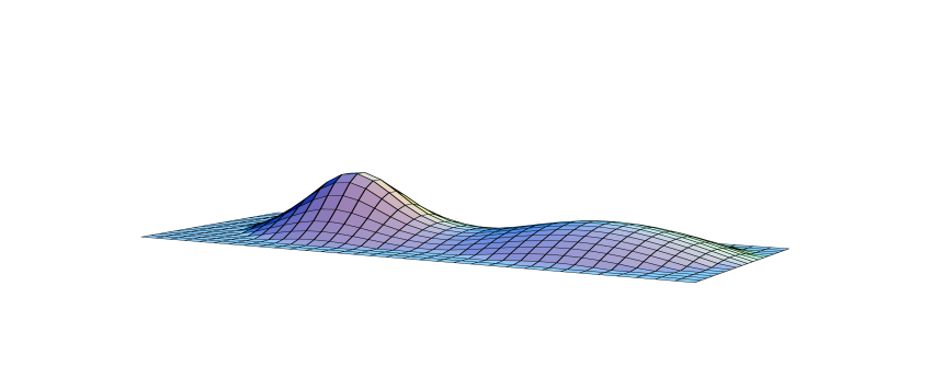
Figure 6: The action density for SU(2) calorons with $\rho=\beta$ and (from left to right) $\mu_{2}=0$ (i.e. trivial holonomy), 0.125 and 0.25 (i.e. ${\rm Tr}{{\cal P}_{\infty}}=0$), at $t=0$ in a plane through the constituent locations.

Important is that when coinciding eigenvalues occur at infinity, that is in ${{\cal P}_{\infty}}$, some constituent masses will vanish. For trivial holonomy only the $n$th constituent is massive and the action density shows a single lump, the usual (deformed) instanton, cmp. Fig. 6. In the presence of massless constituents one cannot take the far field limit, due to the infinite range of the fields in these massless cores. One may, however, move massless constituents off to infinity. For SU(2) this requires one to take $\rho\to\infty$, and one is left with a BPS monopole in a singular gauge to adjust the mismatch in boundary conditions between caloron and monopole, or put differently, to compensate for the magnetic charge that is pushed past infinity [9].

As we have explained in the introduction, chiral zero-modes play an extremely important role in the physics of instantons. They will also turn out to be very useful as a diagnostic tool for studying the properties of the caloron solutions. The Atiyah-Index theorem has taught us there is one chiral zero-mode for a charge 1 caloron. But when the caloron has “dissociated” in $n$ constituents the natural question is if the zero-mode is going to follow this. There is a compelling reason to expect it will opt for being localized on one constituent only. When well separated, the constituents become BPS monopoles. These are known to have zero-modes, but only for a given range of $z$ values in terms of the Higgs expectation value, as dictated by the Callias index theorem [40]. We will show how this determines to which constituent the zero-mode will be localized. Even more useful is that we can change this by introducing an arbitrary phase in the boundary conditions for the fermions, which reads in the algebraic gauge (Eq. (3))

$$\hat{\Psi}_{z}(t+\beta,\vec{x})=\exp(2\pi iz\beta){{\cal P}_{\infty}}\hat{\Psi}_{z}(t,\vec{x}).$$ (55)

Physical fermions at finite temperature are required to be anti-periodic, $\Psi(t,\vec{x})=\hat{\Psi}_{z=1/2\beta}(t,\vec{x})$. That $z$ determines the location of the zero-mode is seen as follows. The gauge transformation $g(t)=\exp(2\pi izt)\exp(tA^{\infty}_{0})$ makes the fermions periodic at the expense of changing $A_{0}=0$ at spatial infinity to $A_{0}=A^{\infty}_{0}-2\pi iz$, cmp. Eq. (5). This acts as an effective mass term in the Dirac equation, which differs for each of the gauge components.

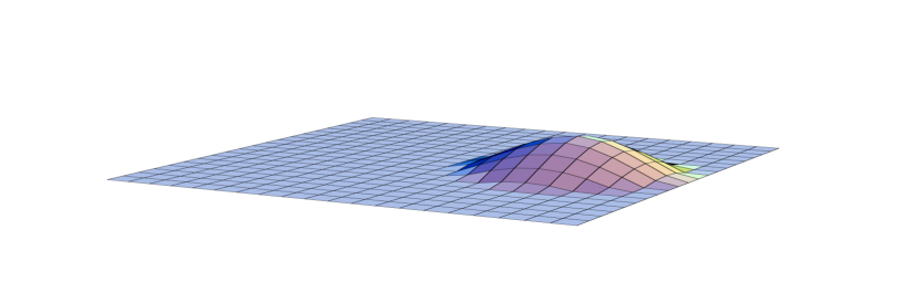
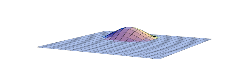
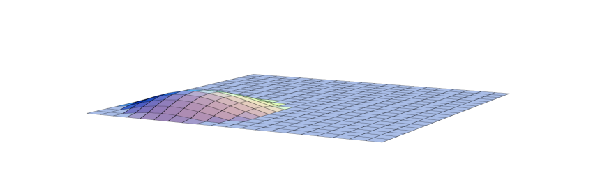
$z=12/60$                       $z=30/60$                       $z=48/60$
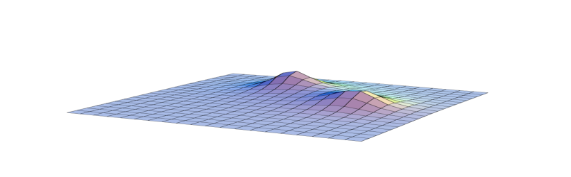
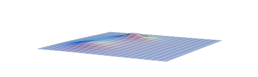
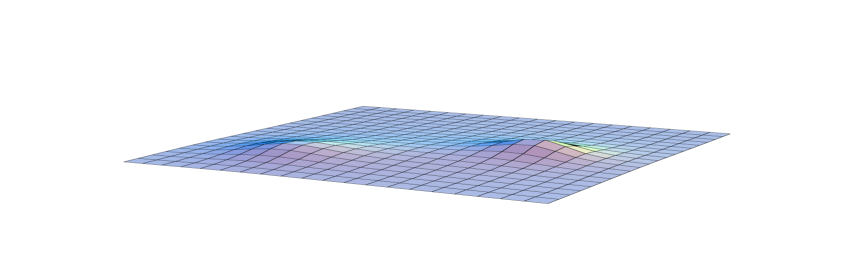
 $z=19/60$                       $z=43/60$                       $z=58/60$

Figure 7: Normalized zero-mode densities at $\beta=1$, for the $SU(3)$ caloron of Fig. 5 shown for $z=\mu_{j}$ on equal linear scales (bottom) and on equal logarithmic scales for three values of $z$ roughly in the middle of each interval $z\in[\mu_{j},\mu_{j+1}]$ (top). The zero-mode with anti-periodic boundary conditions is found at $z=30/60$.

As discussed earlier in this section, each constituent monopole is associated with an SU(2) embedding and the two isospin components of these embeddings effectively have “masses” $2\pi(\mu_{m}/\beta-z)$ and $2\pi(\mu_{m+1}/\beta-z)$. This only gives a normalizable zero-mode when these are of opposite sign [40], that is for $z\in[\mu_{m}/\beta,\mu_{m+1}/\beta]$. In the interior of this interval the zero-mode is exponentially localized (to the constituent monopole at $\vec{y}_{m}$), but at $z=\mu_{m}$ or $z=\mu_{m+1}$ one of the isospin components becomes massless and the zero-mode delocalizes, having in addition support on the constituent at respectively $\vec{y}_{m-1}$ or $\vec{y}_{m+1}$.

The expression for the zero-mode density can be given in a simple form for arbitrary charge 1 calorons as well [41]. With $\mu_{m}/\beta\!\leq\!z^{\prime}\!\leq\!z\!\leq\!\mu_{m+1}/\beta$

$$\hskip-8.53581pt\hat{f}_{x}(z,z^{\prime})=\frac{\pi e^{2\pi it(z-z^{\prime})}}{\beta r_{m}\psi}\langle v_{m}(z^{\prime})|{\cal{A}}_{m\!-\!1}\cdots{\cal{A}}_{1}{\cal{A}}_{n}\cdots{\cal{A}}_{m}-e^{-2\pi it/\beta}|\sigma_{2}v_{m}(z)\rangle,$$

$$\hskip-8.53581ptv_{m}(z)\equiv\pmatrix{\sinh[2\pi(z-\mu_{m}/\beta)r_{m}]\cr\cosh[2\pi(z-\mu_{m}/\beta)r_{m}]\cr},\quad|\hat{\Psi}_{z}(x)|^{2}=-\frac{1}{4\pi^{2}}\partial_{\mu}^{2}\hat{f}_{x}(z,z),$$ (56)

where for later use we have introduced also the off-diagonal expression for the Green’s function $\hat{f}_{x}(z,z^{\prime})$ (for $z\!\leq\!z^{\prime}$ one can use the fact that $\hat{f}_{x}(z^{\prime},z)=\hat{f}_{x}^{*}(z,z^{\prime})$), which can be computed using impurity scattering calculations in a piecewise constant potential, see Sec. 2.3, the details of which need not concern us here. We illustrate the behavior of the zero-mode in Fig. 7 at various values of $z$ for the caloron of Fig. 5. It is also interesting to consider the so-called zero-mode limit (zm) in which $\vec{x}$ is far removed from any constituent location, except the one at $\vec{y}_{m}$. This gives

$$\hat{f}_{x}^{\rm{zm}}(z,z)=\frac{2\pi\sinh\left(2\pi r_{m}(\mu_{m+1}/\beta-z)\right)\sinh\left(2\pi r_{m}(z-\mu_{m}/\beta)\right)}{\beta r_{m}\sinh\left(2\pi r_{m}\nu_{m}/\beta\right)}.$$ (57)

At $z={\scriptstyle{{1\over 2}}}(\mu_{m}+\mu_{m+1})/\beta$ (i.e. $z=0$ or $z=1/2\beta$ for SU(2)) we find

$$\hat{f}_{x}^{\rm{zm}}(z,z)=\pi(r_{m}\beta)^{-1}\tanh(\pi r_{m}\nu_{m}/\beta),$$ (58)

with $-(4\pi^{2})^{-1}\partial_{\mu}^{2}\hat{f}^{\rm{zm}}_{x}(z,z)$ giving precisely the zero-mode density of a basic BPS monopole, confirming once again the nature of the constituents. In the high temperature limit, as long as $z\neq\mu_{m}/\beta$, the zero-modes become infinitely localized to the constituent locations $\vec{y}_{m}$. In this limit the zero-mode density is given by $\beta^{-1}\delta(\vec{x}-\vec{y}_{m})$ for $\mu_{m}/\beta\!<\!z\!<\!\mu_{m+1}/\beta$. The zero-modes are therefore ideal for localizing the cores of the constituent monopoles, particularly useful for the higher charge calorons discussed below. It should be noted that in general the definitions of the constituent locations based on the peaks in the energy density, the degeneracy of two eigenvalues in the Polyakov loop and the peak in the zero-mode densities will only coincide with $\vec{y}_{m}$ when all constituents have a non-zero mass and are well separated (as compared to the size of the monopole cores) from each other.

Before discussing the higher charge calorons we give the simple expression for the SU(2) charge 1 gauge field in the algebraic gauge with ${{\cal P}_{\infty}}=\exp(\beta\omega\tau_{3})$ (hence $\mu_{2}=-\mu_{1}=\beta\omega$),

$$A_{\mu}=\frac{i}{2}\bar{\eta}^{3}_{\mu\nu}\tau_{3}\partial_{\nu}\log\phi+\frac{i}{2}\phi{\rm Re}\left((\bar{\eta}^{1}_{\mu\nu}-i\bar{\eta}^{2}_{\mu\nu})(\tau_{1}+i\tau_{2})\partial_{\nu}\chi\right),$$ (59)

where $\phi^{-1}\equiv 1-\rho^{2}\hat{f}_{x}(\omega,\omega)$ and $\chi\equiv\rho^{2}\hat{f}_{x}(\omega,-\omega)$, which has some resemblance to the ’t Hooft ansatz in Eq. (13). It reduces to this ansatz for trivial holonomy, $\omega=0$, for which $\chi=1-\phi^{-1}$, and one easily checks that this gives precisely the Harrington-Shepard solution with $\phi=\phi_{HS}$, see Eq. (14). In the high temperature limit one finds for non-trivial holonomy $\chi^{\rm{ff}}=0$, $\phi^{\rm{ff}}=(|\vec{x}-\vec{y}_{1}|+|\vec{x}-\vec{y}_{2}|+|\vec{y}_{2}-\vec{y}_{1}|)/(|\vec{x}-\vec{y}_{1}|+|\vec{x}-\vec{y}_{2}|-|\vec{y}_{2}-\vec{y}_{1}|)$ and that $A_{\mu}=\frac{i}{2}\bar{\eta}^{3}_{\mu\nu}\tau_{3}\partial_{\nu}\log\phi^{\rm{ff}}$ describes a pair of oppositely charged Dirac monopoles with the Dirac string on the line connecting them, where $\phi^{\rm{ff}}$ diverges, but outside of which $\log\phi^{\rm{ff}}$ is harmonic.

3.1 Higher charge calorons

When ignoring charged components of the gauge field, outside the core the Abelian field has unavoidable Dirac strings. We can trace how the exact solution instead takes care of the return flux, namely through the Abelian component in the magnetic field coming from the commutator of the charged components of the non-Abelian field, as is of course well-known from the ’t Hooft-Polyakov monopole.

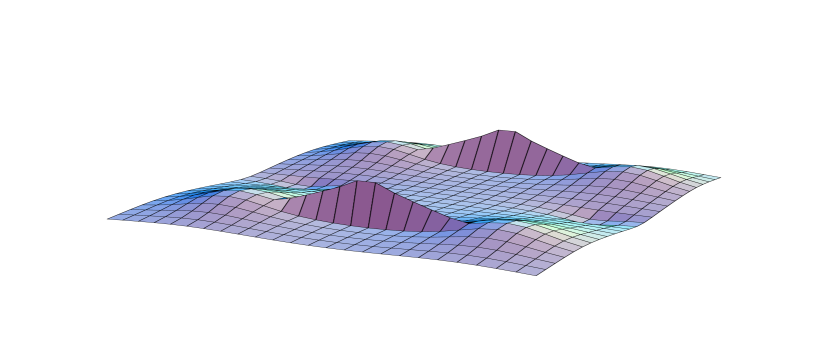
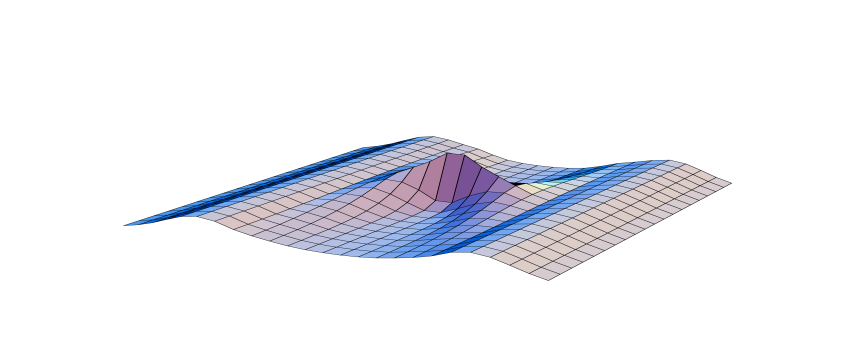
Figure 8: Approximate superposition of two $SU(2)$ charge 1 calorons (left). The logarithm of the action density is plotted through the plane of the constituents at $t=0$ for $\beta=1$ we zoom in by a factor 40 for the transverse direction on the would-be Dirac strings (right).

But from the numerical point of view this will require exponential fine tuning outside the core. It is notoriously difficult to find approximate superpositions for magnetic monopoles without seeing a remnant of the Dirac string, and in that sense there is “no free lunch”. Like in the instanton liquid we would like to make approximate superpositions of calorons, which also allows us to mix calorons of different charges. However, for those that “dissociate”, the constituents should not “remember” from which caloron they originated. Although the constituents themselves might be well separated, interference can occur in the regions between them. An example of this is shown in Fig. 8, where we added two charge 1 caloron gauge fields in the algebraic gauge, called the sum ansatz [20, 21]. This preserves the gauge condition but some care is required at the gauge singularity, which is removed by a gauge transformation with non-trivial winding number (sometimes one refers to these gauge fields as being in the singular gauge). Adding the gauge fields after such a gauge transformation is performed, destroys the proper decay at infinity. Instead, one first smoothly deforms to zero the gauge fields of all other calorons in a small neighborhood centered around the gauge singularity one wishes to remove. This only costs a small amount of action, particularly when the calorons are not too close. In principle a similar construction is possible for keeping Dirac strings hidden, but in this case the gauge singularity is due to approximating the fields by their Abelian component, far from the constituent cores. However, this would require exponential fine tuning. Nevertheless, not performing any adjustment the action density along the Dirac string (or sheet due to the additional extent in the time direction) actually stays finite, see Fig. 8.

It is due to these complications we felt compelled to analyse the higher charge caloron solutions. The disadvantage is that one can only consider the exact self-dual solutions this way, and not superpositions of opposite charges. On the other hand, it should guarantee absence of Dirac strings, as we indeed confirm for a set of exact axially symmetric solutions that share all the properties of the charge 1 solutions, as illustrated for the example of SU(2) charge 2 solutions in Figs. 9-11. In the high temperature limit these solutions are again described by point-like constituent monopoles [26].

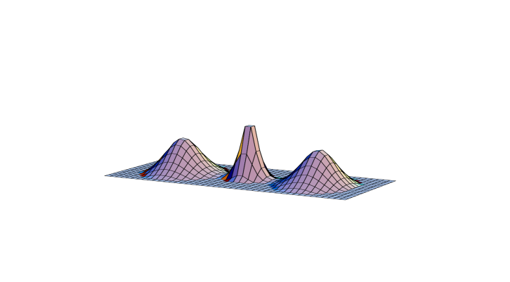
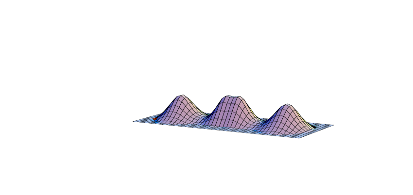
Figure 9: Action density on equal logarithmic scales for exact axially symmetric SU(2) charge 2 solutions at $\beta=1$ for $t=0$, on a plane through the constituents. Locations can be read off from the dotted lines in Fig. 4, from left to right. For the last case see Fig. 11.

Most of the memory effect has disappeared. In the light of this it is interesting to point out that when further separating the two pairs on the left from those on the right, each can be viewed as coming from a single caloron. However, when the two middle constituents start to get closer than the size of their cores, as in Fig. 9 it is more natural to interpret the solution in terms of one well “dissociated” caloron formed by the two outer constituents, on top of which is superposed a small “non-dissociated” caloron, which is no longer static. Indeed, its peak is nearly $O(4)$ symmetric, whereas the other two constituents are static and $O(3)$ symmetric to a high degree, as is appropriate for a BPS monopole (see Fig. 9 (left)).

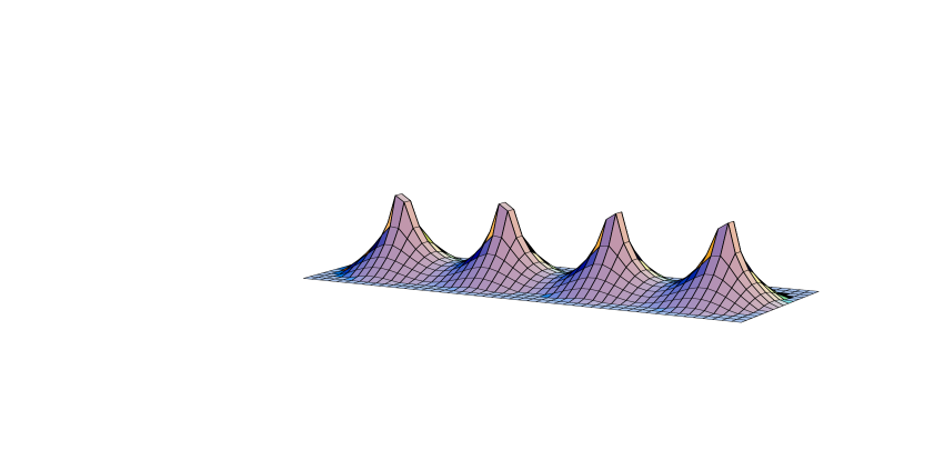
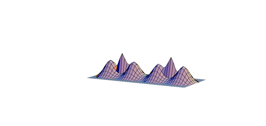
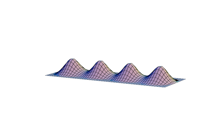
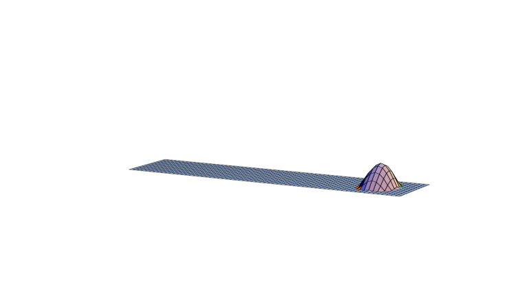
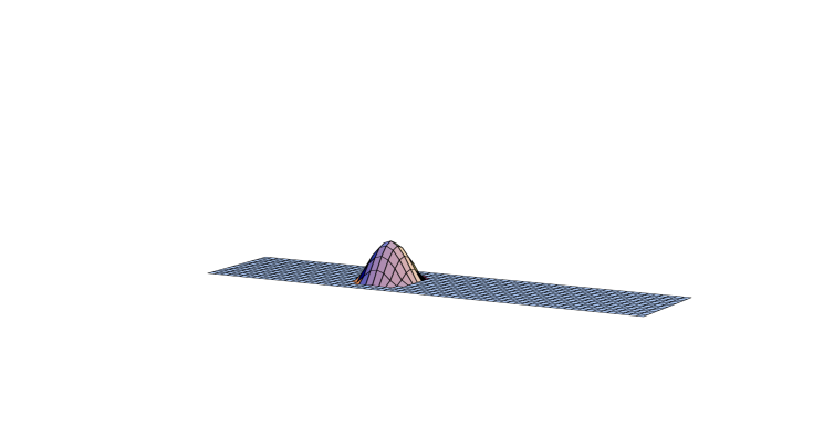
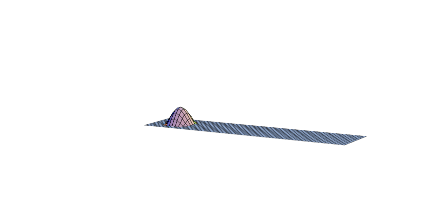
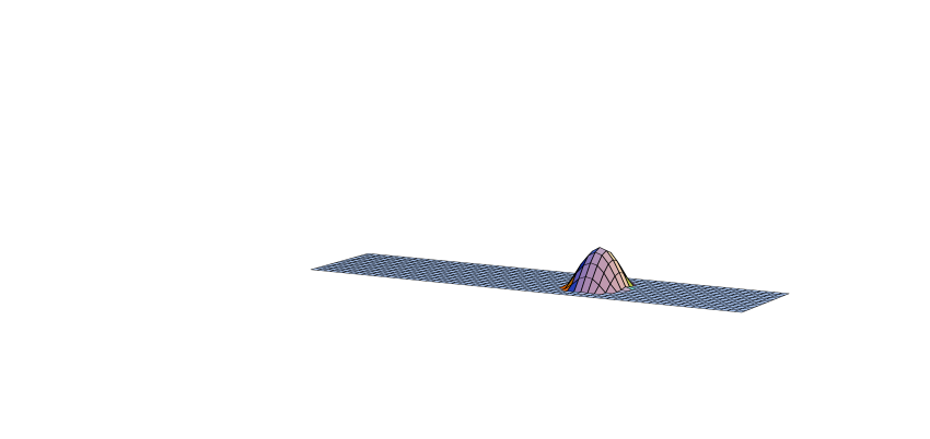
Figure 10: Action density on equal logarithmic scales for the exact axially symmetric SU(2) charge 2 solution with all constituents well-separated (left), the approximate solution based on the sum ansatz (middle) and the high temperature limit with point-like Dirac monopoles (right). See also Fig. 9.

Figure 11: Zero-mode densities on equal logarithmic scales for the caloron in Fig. 11 (same horizontal scale). On the left are shown the two periodic zero-modes ($z=0$) and on the right the two anti-periodic zero-modes ($z=1/2$).

A very subtle memory effect, however, remains. It can be shown that for these point-like axially symmetric solutions the magnetic charges have to alternate. In particular one cannot move one monopole through the other. It may perhaps come as a surprise, but in part there is a good reason for being cautious, since as we have just seen two oppositely charged constituent monopoles really form a small caloron. Since the distance between constituents is given by $\pi\rho^{2}/\beta$, this means that we have to go through a singular caloron when interchanging constituent locations on the line. A singular caloron lies on the boundary of the moduli (i.e. parameter) space and one cannot use continuity arguments.

The reason to expect that in general one no longer deals exclusively with point-like monopoles comes from the known multi-monopole solutions. It is well-known that when putting monopoles of equal charge on top of each other, these are deformed in for example the shape of a doughnut [42], as famously illustrated in the scattering of two magnetic monopoles [43]. At the technical level this is related to the fact that the Green’s function mentioned above no longer involves a piecewise constant potential. Only for the axially symmetric solutions this was still the case. Nevertheless, for SU(2) and charge 2 we have been able to find an exact expression for the zero-mode density in the high temperature limit. As long as $z\neq\mu_{j}$, the fermions have an infinite mass in this limit, and the zero-modes will vanish outside the cores of the constituent monopoles, which themselves need not necessarily be isolated points. We thus are able to trace with the help of the zero-modes to which region the cores have to be localized. Here we will just present the result [31] and discuss its physical significance. For $\mu_{m}\!<\!z\!<\!\mu_{m+1}$ and in the far field limit $\sum_{a}|\hat{\Psi}_{z}^{a}(x)|^{2}=-\beta^{-1}\partial_{i}^{2}{\cal{V}}_{m}(\vec{x})$, with

$${\cal{V}}_{m}(\vec{x})=\frac{1}{2\pi|\vec{x}|}+\frac{{\cal{D}}}{4\pi^{2}}\int_{r<{\cal{D}}}\hskip-14.22636ptdrd\varphi~{}\frac{\partial_{r}|\vec{x}-r\vec{y}(\varphi)|^{-1}}{\sqrt{{\cal{D}}^{2}-r^{2}}},$$ (60)

where $\vec{y}(\varphi)\!=\!(\sqrt{1-{\bf k}^{2}}\cos\varphi,0,\sin\varphi)$, up to an arbitrary coordinate shift and rotation. Here ${\cal{D}}$ is a scale and ${\bf k}$ a shape parameter to characterize arbitrary SU(2) charge 2 solutions. In this representation it is clear that ${\cal{V}}_{m}(\vec{x})$ is harmonic everywhere except on a disk bounded by an ellipse with minor axes $2{\cal{D}}\sqrt{1\!-\!{\bf k}^{2}}$ and major axes $2{\cal{D}}$. Although not directly obvious, when ${\bf k}\to 1$ the support of the singularity structure is on two points only, separated by a distance $2{\cal{D}}$. Taking an arbitrary test function $f(\vec{x})$ one can prove that [31]

$$\lim_{{\bf k}\to 1}-\int f(\vec{x})\partial_{i}^{2}{\cal{V}}_{m}(\vec{x})d^{3}x=f(0,0,{\cal{D}})+f(0,0,-{\cal{D}}).$$ (61)

For the caloron ${\bf k}$ and ${\cal{D}}$ are in general not independent, monopoles of different charges have to adjust to each other to form an exact caloron solution. As an example we illustrate in Fig. 12 the relation for the case studied in Ref. [31], which is a two parameter family of exact SU(2) charge 2 calorons solutions in terms of an instanton scale $\rho$ and relative gauge orientation angle $\alpha$. For fixed $\rho$ it interpolates between two axially symmetric solutions. On the left is shown the relation between ${\bf k}$ and $\rho$ for some values of $\alpha$. Together with the fact that ${\cal{D}}=\pi\sqrt{2}\rho^{2}(1+{\cal{O}}(1-{\bf k}^{2}))$, this shows that ${\bf k}\to 1$ for increasing ${\cal{D}}$. It can be shown this approach is exponential, cmp. Fig. 12 (left).

The important conclusion is that, when well separated, the constituent monopoles become point-like objects.

$~{}{\bf k}$
                                                 $\rho$

Figure 12: On the left we plot ${\bf k}$ versus $\rho$ for $\alpha=0$ (${\bf k}\equiv 1$), $\alpha=-\pi/100$ and $\alpha=-\pi/2$. On the right are shown the locations of the constituent monopoles (fat vs. thin curves for opposite charges) at $\rho=1/4$, varying $\alpha$ from $-\pi$ (indicated by the arrows) to 0.

This is a necessary requirement for the constituent monopoles to be used as entities to describe the field configurations at larger distances. Much work of course remains to be done, but the results so far have been encouraging. In addition important lattice evidence has been accumulated by now, which we will briefly summarize in the next section.

4 Lattice evidence

There are a number of lattice studies, that clearly point to constituent monopoles to have a dynamical role to play. Two methods have been employed. One is based on so-called cooling, the other one uses fermion zero-modes. In both cases the purpose is to filter out ultraviolet noise, i.e. one is interested in the long distance fluctuations.

4.1 Cooling

Cooling is the process by which one lowers the lattice action through local updates, replacing a link by a suitable combination of neighboring links, such that when remaining unchanged it satisfies the lattice equations of motion. There are by now many variants, using improved lattice actions (to reduce discretization errors), and criteria to stop the cooling [44]. Such a criterion is important, because when cooling too long either all the non-trivial fields are removed, or at best one reaches a self-dual solution. The latter is of course sometimes done on purpose, so as to reproduce the classical solutions on the lattice to quite some precision, or to look for solutions not known exactly. For the calorons this has been extensively studied [38], even in connection with a numerical implementation of the Nahm transformation [45], mainly in the presence of so-called twisted boundary conditions [46] to coach the system in having non-trivial holonomy.

From the dynamical point of view, one would like to find how often, and with which properties, calorons appear in the long distance fluctuations. In this case one would like to start from Monte Carlo generated configurations and stop the cooling process when reaching a plateau in the plot for the action as a function of the number of cooling steps. The plateau would be infinitely long if the configuration is a solution of the lattice equations of motion, but would still be sizeable if these are satisfied approximately. Therefore, configurations consisting of any number of well-separated instantons ($Q$) and anti-instantons ($\bar{Q}$) can form such plateaus, with an action approximately equal to $8\pi^{2}(Q+\bar{Q})$, whereas the topological charge of the equivalent continuum configuration equals $Q-\bar{Q}$. An instanton can shrink to such a small size $\rho$ (from the caloron point of view its two constituents monolopes getting too close together) that the lattice no longer supports it as a solution. Also, when instantons and anti-instantons come close together they annihilate, this effect is independent of the lattice discretization. In both cases the plateau ends, and the cooling curve typically settles down at the next plateau where $Q+\bar{Q}$ has decreased by 1 or 2 unit respectively (whereas $Q-\bar{Q}$ changes by $\pm 1$ or 0 respectively). The expectation is that the annihilation of oppositely charged configurations is slow, at least when they are sufficiently separated, and that from the plateaus one can recover the statistical properties of instantons and calorons.

To prompt the system to have a given holonomy, one can freeze the time-like links at the spatial boundary of the box to the required holonomy [48], but in larger volumes it is expected that the confining environment itself will provide local regions with a sufficiently coherent background $A_{0}$ field associated with non-trivial holonomy. One important finding has been that after cooling the non-trivial holonomy is preserved to some degree [49]. This has been analysed for SU(2) in terms of the so-called “asymptotic holonomy” $L_{\infty}$, defined as the average of ${\scriptstyle{{1\over 2}}}{\rm Tr}P(\vec{x})$ over all points $\vec{x}$ for which the action density, summed over $t$, is smaller than .0001. Histograms of $L_{\infty}$ in the confined phase are shown in Fig. 13 (taken from Ref. [49]). Early on in the cooling process a clear peak at $L_{\infty}=0$ is observed, which becomes a flat distribution when cooled down to the plateau associated to $Q+\bar{Q}=1$. Important is in particular that the distribution is not becoming peaked towards $L_{\infty}=\pm 1$. Many configurations with well “dissociated” calorons in this dynamical setting have been found [49], and with this method one can study the configurations in great detail. For SU(2) one can thus look for the monopole centers by finding where the Polyakov loop equals $\pm\Eins_{2}$ and use the fermion zero-modes for periodic and anti-periodic boundary conditions to test if they are localized on the appropriate constituents.

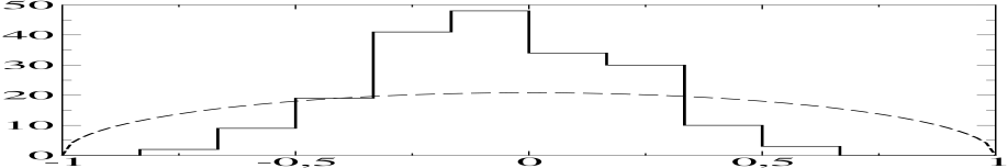
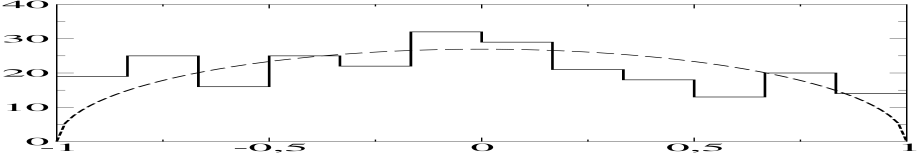
Figure 13: The “asymptotic holonomy” $L_{\infty}$ for an ensemble of ${\cal{O}}(200)$ configurations generated on a $16^{3}\times 4$ lattice with periodic boundary conditions for a lattice coupling $4/e^{2}=2.2$. Left is shown the measurement on the first plateau, right on the last plateau. For comparison the Haar measure $\sqrt{1-L^{2}}$ is shown by the dashed curve. Figures taken from Ref. [49].

In these studies one also finds configurations that cannot be directly interpreted in terms of instantons, calorons and their possible constituent monopoles [49]. Interestingly, there are cases where two constituents appear, but of opposite fractional topological charge. These could arise from the “annihilation” of two other constituents of opposite duality [50] but where originally each of these, together with one of the surviving constituents, formed an (anti-)caloron. More recently these authors also performed cooling studies for SU(2) at considerably lower temperature than just around the deconfining phase transition [51]. The calorons in this case do not tend to “dissociate” in isolated lumps of action density. Nevertheless, constituents could be identified through the behavior of the Polyakov loop and were characteristic for non-trivial holonomy. This may explain why in the past constituent monopoles were never noticed in cooling studies. Finally let us mention that many results for SU(3) have now been obtained as well [51].

4.2 Zero-mode filter

The use of zero-modes as a filter relies on two observations. The first is, as we have seen, that zero-modes quite accurately trace the underlying gauge field of instantons, calorons and constituent monopoles. Secondly, a zero-mode probes the long distance features of the configuration and ignores the ultraviolet high momentum components, otherwise one could never have a zero-mode. In some sense the Dirac operator is a particular projection of the covariant momentum. For SU(3), comparing periodic and anti-periodic fermion boundary conditions [52], or cycling through all possible phases [53], Eq. (55), a significantly different behavior in the two phases was found. In the deconfined phase, the proper $z$-dependent behavior of the trivial holonomy configuration is seen. These are of course the old Harrington-Shepard solutions, but their zero-modes were previously only considered for anti-periodic boundary conditions. In the confined phase indications for a three lump structure is seen (see Fig. 14, taken from Ref. [53]) in a reasonable fraction of the configurations.

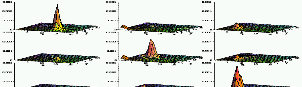
Figure 14: The zero-mode density for a particular configuration in the confined phase on a $6\times 20^{3}$ lattice with (Lüscher-Weisz) coupling $6/e^{2}=8.20$, taken from Ref. [53]. Shown are slices in $(x,y)$ at $(t,z)=(5,9)$ (left), $(t,z)=(2,19)$ (center) and $(t,z)=(5,18)$ (right), for $z=0.05$, 0.3 and 0.65 (from top to bottom).

These results are based on dynamical configurations generated with the Lüscher-Weisz [54] improved lattice action. Configurations that had exactly one chiral zero-mode (which requires the use of a chirally improved lattice Dirac operator [55]) were singled out. By the index theorem, this implies the topological charge is equal to one. The dynamically generated configurations can, and typically will, consist of Q+1 instantons and Q anti-instantons, giving rise to near zero-modes with less perfect chiral behavior. Work is in progress to analyse the near zero-modes, as well as performing cooling on the SU(3) gauge field configurations [56]. This will help to further rule out the unlikely possibility for the zero-mode to jump between instanton, rather than monopole constituents. A more theoretical study [57] has recently shown that it seems indeed impossible for the full signature of a single caloron with non-trivial holonomy to be emulated by the effect of hopping between instantons.

Even more remarkable is that a similar structure of multiple lumps for the topological charge 1 sector was found on a symmetric lattice of size $16^{4}$ and $12^{4}$ at low temperature, well in the confined phase [53, 58]. In this case the lattice does not single out one direction as being (imaginary) time. Yet, using one of these directions to impose the $z$ dependent boundary condition for the fermions, in almost half of the configurations one finds more than one lump. The results seem to indicate these lumps are randomly distributed over the volume. How to reconcile this with the results found with cooling, that pointed to “non-dissociated” calorons at low temperature, is at the moment not clear. But let us recall that fractionally charged instantons on the torus were long ago introduced by ’t Hooft [46], and have been extensively studied on the lattice [60]. Twisted boundary conditions and, related to it, the quantization of the topological charge in units of $1/n$, make it more difficult to embed these solutions in a dynamical environment. Nevertheless, on the basis of some simple assumptions concerning the dynamical properties of these configurations, quasi realistic results have been obtained [61]. It is indeed compelling to interpret the $4kn$ dimensions of the SU($n$) charge $k$ instanton parameter space on the torus in terms of the space-time locations of $kn$ instanton quarks, as they were called long ago [59] (even though their meaning at that time was more abstract). Results for instantons on $T^{2}\times R^{2}$, that in some sense interpolate between the case of calorons and instantons on the torus, give further evidence [62] for this conjecture.

5 Conclusion

It is clear we can do no justice here to all the results that have been obtained in using lattice simulations. The great advantage of using zero-modes as a filter is that it minimizes the bias, since it directly uses the Monte Carlo configurations themselves. On the other hand, in the cooling studies one has access to the relation between the behavior of the Polyakov loop, which plays the role of an order parameter in SU($n$) gauge theories, and the presence of constituent monopoles, which may give some insight in the underlying dynamics. Of course, we would like to make constituent monopoles into a precise tool, e.g. for testing the celebrated idea of a dual superconductor to describe confinement [63, 64], or as we speculated in the introduction, to describe a dense phase of monopoles to lead to deconfinement of magnetic charges, like quark deconfiment at high density.

On the more theoretical side we have also not touched upon the role these constituent monopoles play in supersymmetric gauge theories [65, 67] and how the initial motivation for reconsidering calorons with non-trivial holonomy came from the study of D-branes [8, 35, 66]. Nevertheless, we feel the applications to the dynamics of non-Abelian gauge theories is very promising. We hope to have given the reader some insight in this matter.

References

- [1] B.J. Harrington and H.K. Shepard, Phys. Rev. D17 (1978) 2122; ibid. D18 (1978) 2990.
- [2] D.J. Gross, R.D. Pisarski and L.G. Yaffe, Rev. Mod. Phys. 53 (1981) 43.
- [3] P. van Baal, in: At the Frontiers of Particle Physics – Handbook of QCD, Vol.2, ed. M. Shifman (World Scientific, Singapore, 2001), p. 683 [hep-ph/0008206].
-
[4]
G. ’t Hooft, Nucl. Phys. B79 (1974) 276;
A.M. Polyakov, JETP Lett. 20 (1974) 194. - [5] E.B. Bogomol’ny, Sov. J. Nucl. Phys. 24 (1976) 449; M.K. Prasad and C.M. Sommerfield, Phys. Rev. Lett. 35 (1975) 760.
- [6] N.S. Manton, Nucl. Phys. B126 (1977) 525.
- [7] C. Montonen and D. Olive, Phys. Lett. 72B (1977) 117.
- [8] K.Lee and P. Yi, Phys. Rev. D56 (1997) 3711.
- [9] P. Rossi, Nucl. Phys. B149 (1979) 170.
- [10] B. Julia and A. Zee, Phys. Rev. D11 (1975) 2227.
- [11] T.C. Kraan and P. van Baal, Nucl. Phys. B533 (1998) 627 [hep-th/9805168].
- [12] E. Witten, Phys. Lett. 86B (1979) 283.
- [13] W. Nahm, Self-dual monopoles and calorons, in: Lecture Notes in Physics 201 (1984) 189.
- [14] M.F. Atiyah, N.J. Hitchin, V. Drinfeld and Yu.I. Manin, Phys. Lett. 65A (1978) 185; M.F. Atiyah, Geometry of Yang-Mills fields, Fermi lectures, (Scuola Normale Superiore, Pisa, 1979).
- [15] C. Taubes, Morse theory and monopoles: topology in long range forces, in: Progress in gauge field theory, eds. G. ’t Hooft et al, (Plenum Press, New York, 1984) p. 563.
- [16] T.C. Kraan and P. van Baal, Nucl. Phys. A642 (1998) 229-304 [hep-th/9805201].
- [17] G. ’t Hooft, Phys. Rev. Lett. 37 (1976) 8; Phys. Rev. D14 (1976) 3432; Phys. Rept. 142 (1986) 357.
- [18] C. Taubes, J. Diff. Geom. 17 (1982) 139; ibid. 19 (1984) 517.
- [19] S.K. Donaldson and P.B. Kronheimer, The Geometry of Four-Manifolds, (Clarendon Press, Oxford, 1990).
- [20] T. Schäfer and E.V. Shuryak, Rev. Mod. Phys. 70 (1998) 323; [hep-ph/9610451].
- [21] D. Diakonov, Instantons at work, hep-ph/0212026, to appear in Prog. Part. Nucl. Phys.
- [22] M.F. Atiyah and I.M. Singer, Ann. Math. 87 (1968) 484; ibid. 93 (1971) 119.
- [23] T. Banks and A. Casher, Nucl. Phys. B169 (1980) 103.
- [24] R. Rajaraman, Solitons and Instantons, (North-Holland, Amsterdam, 1982).
- [25] R. Jackiw, C. Nohl, C. Rebbi, Phys. Rev. D15 (1977) 1642.
- [26] F. Bruckmann, P. van Baal, Nucl. Phys. B653 (2002) 105. [hep-th/0209010].
-
[27]
P.J. Braam and P. van Baal, Commun. Math. Phys. 122
(1989) 267;
P. van Baal, Nucl. Phys. B(Proc. Suppl.)49 (1996) 238 [hep-th/9512223]. - [28] E.F. Corrigan, D.B. Fairlie, S. Templeton and P. Goddard, Nucl. Phys. B140 (1978) 31.
- [29] H. Osborn, Ann. Phys. (N.Y.) 135 (1981) 373; Nucl. Phys. B159 (1979) 497.
- [30] M. García Pérez, A. González-Arroyo, C. Pena and P. van Baal, Phys. Rev. D60 (1999) 031901 [hep-th/9905016].
- [31] F. Bruckmann, D. Nógrádi, P. van Baal, Nucl. Phys. B666 (2003) 195 [hep-th/0305063].
-
[32]
S.A. Brown, H. Panagopoulos and M.K. Prasad,
Phys. Rev. D26 (1982) 854; H. Panagopoulos, Phys. Rev. D28 (1983) 380;
A.S. Dancer, Comm. Math. Phys. 158 (1993) 545. - [33] T.C. Kraan and P. van Baal, Phys. Lett. B435 (1998) 389 [hep-th/9806034].
-
[34]
K. Lee, Phys. Lett B426 (1998) 323 [hep-th/9802012];
K. Lee and C. Lu, Phys. Rev. D58 (1998) 025011 [hep-th/9802108]. - [35] T.C. Kraan and P. van Baal, Phys. Lett. B428 (1998) 268 [hep-th/9802049].
- [36] T.C. Kraan, Comm. Math. Phys. 212 (2000) 503-533 [hep-th/9811179].
- [37] P. van Baal, in: Lattice fermions and structure of the vacuum, eds. V. Mitrjushkin and G. Schierholz (Kluwer, Dordrecht, 2000), p. 269 [hep-th/9912035].
- [38] M. García Pérez, A. González-Arroyo, A. Montero and P. van Baal, JHEP 06 (1999) 001 [hep-lat/9903022].
- [39] P. van Baal, Nucl. Phys. B(Proc.Suppl.)106 (2002) 586 [hep-lat/0108027]; Nucl. Phys. B(Proc.Suppl.)108 (2002) 3 [hep-th/0109148].
- [40] C.J. Callias, Comm. Math. Phys. 62 (1978) 213.
- [41] M.N. Chernodub, T.C. Kraan, P. van Baal, Nucl. Phys. B(Proc.Suppl.)83-84 (2000) 556.
- [42] P. Forgács, Z. Horváth and L. Palla, Nucl. Phys. B192 (1981) 141;
- [43] M.F. Atiyah and N.J. Hitchin, The Geometry and Dynamics of Magnetic Monopoles, (Princeton Univ. Press, 1988).
- [44] M. García Pérez, O. Philipsen and I.O. Stamatescu, Nucl. Phys. B551 (1999) 293 [hep-lat/9812006].
-
[45]
A. González-Arroyo and C. Pena, JHEP 09 (1998) 013
[hep-th/9807172];
M. García Pérez, A. González-Arroyo, C. Pena and P. van Baal, Nucl. Phys. B564 (2000) 159 [hep-th/9905138]. - [46] G. ’t Hooft, Nucl. Phys. B153 (1979) 141.
- [47] M. García Pérez, A. González-Arroyo, J. Snippe and P. van Baal, Nucl. Phys. B413 (1994) 535-553 [hep-lat/9309009].
-
[48]
E.-M. Ilgenfritz, M. Müller-Preussker and A.I. Veselov,
in: Lattice fermions and structure of the vacuum, eds. V. Mitrjushkin
and G. Schierholz (Kluwer, Dordrecht, 2000), p. 345 [hep-lat/0003025];
E.-M. Ilgenfritz, B. Martemyanov, M. Müller-Preussker and A.I. Veselov, Nucl. Phys. B(Proc. Suppl.)94 (2001) 407 [hep-lat/0011051]. - [49] E.-M. Ilgenfritz, B.V. Martemyanov, M. Müller-Preussker, S. Shcheredin and A.I. Veselov, Phys. Rev. D66 (2002) 074503.
- [50] E.-M. Ilgenfritz, B.V. Martemyanov, M. Muller-Preussker and A.I. Veselov, Nucl. Phys. B(Proc. Suppl.)106 (2002) 589 [hep-lat/0110212].
- [51] E.-M. Ilgenfritz, talk presented at Lattice 2003, Tsukuba, July 2003.
- [52] C. Gattringer, Phys. Rev. D67 (2003) 034507 [hep-lat/0210001].
- [53] C. Gattringer and S. Schaefer, Nucl. Phys. B654 (2003) 30. [hep-lat/0212029].
- [54] M. Lüscher and P. Weisz, Commun. Math. Phys. 97 (1985) 59.
- [55] C. Gattringer, Phys. Rev. D63 (2001) 114501 [hep-lat/0003005]; C. Gattringer, I. Hip, C.B. Lang, Nucl. Phys. B 597 (2001) 451 [hep-lat/0007042].
- [56] C. Gattringer, M. Ilgenfritz, B. Martemyanov and M. Müller-Preussker, private communication.
- [57] F. Bruckmann, D. Nógrádi, M.García Pérez and P. van Baal, hep-lat/0308017, to appear in the proceedings of Lattice 2003, Tsukuba, July 2003.
- [58] C. Gattringer, talk presented at Lattice 2003, Tsukuba, July 2003.
- [59] A.A. Belavin, V.A. Fateev, A.S. Schwarz and Y.S. Tyupkin, Phys. Lett. B83 (1979) 317.
- [60] M. García Pérez, A. González-Arroyo, J. Phys. A26 (1993) 2667 [hep-lat/9206016]; M.García Pérez, PhD. Thesis, Univ. Atonoma de Madrid (1992).
- [61] A. Gonzalez-Arroyo and P. Martínez, Nucl. Phys. B459 (1996) 337 [hep-lat/9507001]; A. González-Arroyo and P. Martínez and A. Montero, Phys. Lett. B359 (1995) 159 [hep-lat/9507006].
- [62] C. Ford and J. Pawlowski, Phys. Lett. B540 (2002) 153 [hep-th/0205116]; Doubly Periodic Instantons and their Constituents, hep-th/0302117.
- [63] S. Mandelstam, Phys. Rept. 23 (1976) 245.
- [64] G.’t Hooft, in: High Energy Physics, ed. A. Zichichi (Editrice Compositori, Bolognia, 1976); Nucl. Phys. B138 (1978) 1.
- [65] N.M. Davies, T.J. Hollowood, V.V. Khoze and M.P. Mattis, Nucl. Phys B559 (1999) 123 [hep-th/9905015].
- [66] K. Lee and P. Yi, Phys. Rev. D58 (1998) 066005 [hep-th/9804174].
- [67] D. Diakonov and V. Petrov, Phys. Rev. D 67 (2003) 105007 [hep-th/0212018].