We give a full nonlinear numerical treatment of time-dependent 5d braneworld geometry, which is determined self-consistently by potentials for the scalar field in the bulk and at two orbifold branes, supplemented by boundary conditions at the branes. We describe the BraneCode${}^{\mbox{\textregistered}}$, an algorithm which we designed to solve the dynamical equations numerically. We applied the BraneCode to braneworld models and found several novel phenomena of the brane dynamics.
Starting with static warped geometry with de Sitter branes, we found numerically that this configuration is often unstable due to a tachyonic mass of the radion during inflation. If the model admits other static configurations with lower values of de Sitter curvature, this effect causes a violent re-structuring towards them, flattening the branes, which appears as a lowering of the 4d effective cosmological constant.
Braneworld dynamics can often lead to brane collisions. We found that in the presence of the bulk scalar field, the 5d geometry between colliding branes approaches a universal, homogeneous, anisotropic strong gravity Kasner-like asymptotic, irrespective of the bulk/brane potentials. The Kasner indices of the brane directions are equal to each other but different from that of the extra dimension.

1 Introduction

Braneworlds embedded in higher dimensions bring new powerful concepts in cosmology [1], as well as they do in fundamental superstring/M theories and phenomenological high energy particle physics [2, 3, 4, 5]. Branes enrich our view with new ideas underlying the four dimensional effective field theory, bringing, most importantly, new geometrical images beyond it. For instance, in this context the four dimensional cosmological constant is the curvature of the brane, and we should explain why the brane we live in is almost flat. Inflation, by contrast, corresponds to curved branes. There are interesting ideas for realizing early universe inflation in braneworld scenarios where, for example, concepts such as the inflaton potential and inflaton decay are reformulated in terms of brane-brane or brane-antibrane interactions [6], or topics of brane collisions.

The language and images of the braneworld theories are commonly shared by fundamental and phenomenological high energy physics theories, general relativity and brane cosmology, with different degrees of trade between dynamics and simplification.

The compactification of the extra space is often a key issue in brane models. For example, a stable radion field, controlling the volume of the extra space, is usually needed to recover standard four dimensional cosmology at “late” times, and to fulfill precision tests of general relativity. In addition, the compactification has to be consistent with the fact that bulk fields have not yet been excited in accelerator experiments, because they are too massive and/or too weakly coupled to the visible brane. Schemes for compact inner dimensions typically rely on the interplay between bulk and brane dynamics.

So far, the control of dynamical, time-dependent, cosmologically relevant solutions in the fundamental, comprehensive theory has been rather limited. Relatively simple, yet meaningful, are the five dimensional phenomenological braneworld models with two orbifold branes at the edges, where our $3+1$ dimensional spacetime is one of the branes embedded in the (warped) five dimensional space. These models often include one or more bulk scalar field(s) $\phi$ with the potential $V(\phi)$ and self-interaction potentials $U_{i}(\phi)$ at the two branes, as well as other fields $\chi$ localized at the branes. This class of braneworld models covers many interesting constructions including the Hořava-Witten theory [3], the Randall-Sundrum model with a phenomenological stabilization of branes [7, 8], warped geometry with bulk scalars [10, 20], supergravity with domain walls [9], and others.

There is a number of important papers studying static geometries with branes, including flat stabilized branes, in agreement with low energy physics, curved de Sitter branes, corresponding to early universe inflation, and small fluctuations around static warped geometries. The cosmological evolution has been studied in some of these pioneering works in the simplest cases in the absence of any scalar field [12, 13]. The 4d evolution on the brane, in terms of effective Friedmann equations, is typically different from the standard four dimensional cosmology. The effective 4d Einstein equations on the brane were also derived for the more general situation of self-consistent geometry with the bulk/brane scalar field [14].

Standard cosmology can be recovered after the extra dimensions have been stabilized [11]. In this respect, the presence of bulk scalar field(s) becomes crucial. In this more relevant case, however, the evolution is only known for limiting situations. In general, the system is very complicated, since the effective four dimensional Einstein equations are not closed and require solutions of the full five dimensional equations [31].

In this paper we address the problem of self-consistent fully nonlinear dynamics of the 5d braneworld with bulk scalar field(s) with a bulk potential as well as brane potentials required for brane stabilization. We consider plane-parallel orbifold branes, so that the problem is effectively two dimensional, with the metric and the fields depending on time and the extra dimension $(t,y)$. Although this setting is already too involved to be studied analytically, it is still significantly simpler than what we will need in order to understand cosmological solutions in “realistic” higher dimensional theories. However, as we shall see, already this step requires the introduction of new techniques. We have designed and used a numerical code to solve the partial differential equations describing the system of non-linear gravity and a scalar field, complementing the existing approaches to this problem found in the literature.

We aim for generic features of braneworld dynamics, in particular, attractor solutions. They will generally depend on the specific braneworld model, i.e. on the bulk/brane scalar field potentials $V(\phi),U_{i}(\phi)$. As a simple illustration, consider a static five-dimensional warped geometry with a bulk scalar and four dimensional slices of constant curvature. It is possible to exhaust the global properties of static warped geometry using the method of phase trajectories [17], although some details of the phase portraits depend on the bulk potential. For this problem the phase space is three dimensional, the critical points (like attractors, repulsors, and others) can be identified, and all trajectories (solutions) start and end at critical points.

The $(t,y)$ problem of the time-dependent braneworld dynamics is much more complicated than the static $(y)$ problem. Using the BraneCode we were trying to give examples of interesting dynamical features. We notice several novel phenomena including a transition between different warped states and a generic strong gravity solution of colliding branes.

The plan of the paper is the following.

In Section 2, we give the setup of the braneworld models and write down the bulk equations supplemented by the junction conditions at the branes. We pay especially close attention to the choice of the gauge in order to have a suitable metric for the numerical calculations. It turns out that, without any loss of generality, it is possible to choose coordinates where the two branes have fixed positions along the fifth direction $y$. The geometry is described by two metric components $A(t,y)$ and $B(t,y)$.

In Section 3, we describe the BraneCode, an algorithm we use to solve the dynamical equations numerically. At the moment we have slightly different implementations of the BraneCode (in $C++$ and Fortran$-90$) in order to cross-check them. We plan to release the BraneCode using the most optimized and documented version (in $C++$). As is typical for numerical GR problems, we have to take initial conditions for the metric and fields which satisfy the constraint equations at an initial time hypersurface. In Subsection 3.3, we discuss how to fix the initial conditions for the numerical integration with the BraneCode.

In Sections 4–6, we apply our BraneCode to three braneworld models where we encounter qualitatively different dynamics.

In order to check our numerical code, in Section 4 we first apply it to a simpler brane model without a scalar field, for which analytic solutions are known. As a playground here we use the Randall-Sundrum model of two branes embedded in an AdS 5d background. In Subsection 4.1 we first use the static RS solution without moving branes. In Subsection 4.2 we extend the calculations to the case of moving branes. In this case the 5d geometry is described by the analytic AdS-Schwarzschild solution (with the mass of the virtual 5d black-hole screened by the branes). We compare our numerical calculations with the analytic solution.

In Section 5 we consider de Sitter (inflating) branes which are initially in a static configuration. It turns out that we often observe an instability of the inflating branes. Analytic calculations of small scalar perturbations around this background geometry show that the radion mass square $m^{2}$ for this case can be negative [16]. A strong tachyonic instability predicted analytically is in full agreement with the instability of inflating branes found numerically. For certain configurations of potentials $V(\phi),U_{i}(\phi)$, we find the existence of two warped geometry solutions with different values of the 4d cosmological constant $\Lambda_{4}$ (i.e. the curvatures of the 4d slices). The brane configuration with the higher 4d curvature is in general unstable due to this tachyonic radion mode, and violently re-configures to the second static configuration with lower 4d curvature. We illustrate this effect with numerical simulations as well as analytic calculations, see also [16].

In Section 6 we give an example where the instability of the brane configuration causes a brane collision. In Subsection 6.1 we show that the space-time metric of the 5d geometry between colliding branes becomes homogeneous, i.e. $y$-independent. The time-dependent solutions asymptotically cease to feel the scalar field potentials $V(\phi)$ and $U_{i}(\phi)$, and approach a universal asymptotic. It sounds natural a posteriori that this universal asymptotic is nothing but a Kasner-like asymptotic with a scalar field, which we describe in Subsection 6.2. The effect of the branes here is manifested by the fact that the Kasner indices associated with the three brane directions are equal, but different from that associated with the $y$ direction. This is a strong gravity regime, so it is not surprising that the 4d induced metric on the brane is different from that derived with moduli approximations in terms of 4d effective theory.

In the Conclusion we summarize the most interesting physical results. Technical details are collected in several Appendices.

2 Setup

The class of braneworld models we are interested in is characterized by the following action

$$\kappa_{5}^{2}\,S = \frac{1}{2}\int d^{5}x\sqrt{-\,g}\,R+\int d^{5}x\sqrt{-g}\,\left[-\,\frac{1}{2}\left(\partial\phi\right)^{2}-V\left(\phi\right)\right]+$$ (1)

$$- \sum_{i=1,2}\int_{b_{i}}d^{4}x\sqrt{-\,\gamma}\,\left\{\left[K\right]+{U}_{i}\left(\phi\right)\right\}\,\,,$$

where $\kappa_{5}^{2}=\frac{1}{M_{5}^{3}}$ is a 5d gravitational constant. In this convention $\phi$ is measured in units of $\kappa_{5}^{-1}$ and physical potentials are multiplied by $\kappa_{5}^{-2}$. The first term describes gravity in the five dimensional bulk space. We use the “mostly positive” metric signature. The second term corresponds to a (minimally coupled) bulk scalar field with the potential $V(\phi)$. The last term corresponds to two $3+1$ dimensional branes, which constitute the boundary of the five dimensional space. We allow for a potential term ${U(\phi})$ for the scalar field at each of the two branes. We denote by $\gamma$ the induced metric on the two branes, and by $K$ their extrinsic curvature. Here and in the following, $\left[Q\right]\equiv Q\left(y_{+}\right)-Q\left(y_{-}\right)$ denotes the jump of any quantity $Q$ across a brane ($\pm$ defined respect to the normal of the brane). We assume $S^{1}/{\mathbb{Z}}_{2}$ symmetry across each brane.

The algorithm we have written is implemented for generic bulk and brane potentials. In this paper we specify the potentials introduced for the brane stabilization [7]. We choose

$$V(\phi) = \frac{1}{2}\,m^{2}\phi^{2}+\Lambda\,\,,$$

$${U}_{i}(\phi) = \frac{1}{2}M_{i}\left(\phi_{i}-\sigma_{i}\right)^{2}+\lambda_{i}\,\,,$$ (2)

where $\phi_{i}$ is the value of $\phi$ on the $i-$th brane. A 5d cosmological constant $\Lambda$ in the bulk and tensions $\lambda_{i}$ on the branes are included in the potentials.

The two branes are assumed to be parallel. We denote by $y$ the coordinate transverse to them, and by ${\bf x}$ the three spatial longitudinal coordinates. We assume isometry along three dimensional ${\bf x}$ slices including the branes. We have to specify a metric $g_{AB}$ that respects this symmetry. In brane cosmology it is customary to use the metric in the form $ds^{2}=-n^{2}dt^{2}+a^{2}d{\bf x}^{2}+bdy^{2}$, where the metric components $n,a,b$ depend on $(t,y)$. However, this form of metric does not exhaust the freedom of the coordinate choices. Most significantly, in this metric the branes do not stay at the fixed positions; in general $y_{i}=y_{i}(t)$. There are other gauge choices, which were used for specific braneworld problems, for example coordinates comoving with one of the branes, the choice of the bulk scalar $\phi$ as the $y$-hypersurface and others. In these contexts, a gauge in which the position of one of the two branes is time dependent was often preferred, and identified with the radion field ${\cal R}\left(t\right)$ associated with the extra dimension. Although this choice may lead to an easier interpretation of the interbrane distance, the resulting bulk and junction conditions (see below) are significantly more complicated. In addition, in terms of the four dynamical quantities $a,b,n,\phi,$ and ${\cal R}\,$ the system is actually under-determined, and some gauge fixing is needed to have a closed set of equations.

For numerical simulations, it is preferable to have coordinates where neither brane is moving, although it is not obvious a priori that such a gauge can be constructed without loss of generality. It is possible to choose coordinates such that the bulk metric has the “2d conformal gauge”,

$$ds^{2}={\rm e}^{2\,B\left(t,y\right)}\left(-dt^{2}+dy^{2}\right)+{\rm e}^{2\,A\left(t,y\right)}\,d{\bf x}^{2}\,\,,$$ (3)

This gauge still has the residual freedom to change $(t,y)\to(t^{\prime},y^{\prime})$ in a way that preserves the 2d conformal form. It can be demonstrated that this freedom can be used to fix the position of the two branes along $y\,$. Without loss of generality, we can locate them at $y=0,1\,$. We found that in the 2d conformal gauge the set of bulk equations (5) acquires a relatively simple form, which is well suited for the numerical scheme we have adopted (see the next section). The possibility of choosing a gauge, in which the metric is 2d conformal and in which the branes are at a fixed position is shown explicitly in Appendix A.1. As it is discussed in Appendix A.2, even these requirements do not fix the gauge choice completely.

Although in the system of coordinates we have chosen the branes are always at a fixed position along the $y$ axis, their physical distance is encoded in the metric component $B\,$, which is a time dependent quantity. Clearly, the distance between two extended objects is not an invariant quantity in general relativity, and different definitions can be adopted when they are in relative motion. A simple heuristic possibility, which we adopt here, is to integrate the line element across the extra dimension at a fixed time

$$D\left(t\right)\equiv\int_{0}^{1}dy\,\sqrt{g_{55}}=\int_{0}^{1}dy\,{\rm e}^{B\left(t,\,y\right)}\ .$$ (4)

One can check that $D\left(t\right)$ is invariant under the residual gauge freedom in our coordinates (3), which is discussed in Appendix A.2 (but not under general coordinate transformations).

For the output of our numerical calculations, we rely on gauge invariant quantities such as the invariants of the 5d Weyl tensor $C_{ABCD}C^{ABCD}$, the curvature scalar $R$ and others. These invariants are calculated using the metric in the form (3). Additionally, we can use the $4+1$ split of the 5d curvature, symbolically written as $R=R_{4}+K^{2}$, where $R_{4}$ is the curvature of the 4d slices. This will be especially useful when we work with de Sitter (inflating) branes of constant curvature.

In the gauge we have chosen, the nontrivial five-dimensional Einstein equations can be split into three dynamical equations

$$\ddot{A}-A^{\prime\prime}+3\dot{A}^{2}-3A^{\prime 2}=\frac{2}{3}\,{\rm e}^{2B}V\,\,,$$

$$\ddot{B}-B^{\prime\prime}-3\dot{A}^{2}+3A^{\prime 2}=-\frac{\dot{\phi}^{2}}{2}+\frac{\phi^{\prime 2}}{2}-\frac{1}{3}{\rm e}^{2B}V\,\,,$$

$$\ddot{\phi}-\phi^{\prime\prime}+3\dot{A}\dot{\phi}-3A^{\prime}\phi^{\prime}+{\rm e}^{2B}V_{,\phi}=0\,\,,$$ (5)

plus two constraint equations

$$-A^{\prime}\dot{A}+B^{\prime}\dot{A}+A^{\prime}\dot{B}-\dot{A}^{\prime}=\frac{1}{3}\,\dot{\phi}\,\phi^{\prime}\,\,,$$

$$2A^{\prime 2}-A^{\prime}B^{\prime}+A^{\prime\prime}-\dot{A}^{2}-\dot{A}\dot{B}=-\frac{\dot{\phi}^{2}}{6}-\frac{\phi^{\prime 2}}{6}-\frac{1}{3}\,{\rm e}^{2B}V\,\,.$$ (6)

Dots and primes denote derivatives with respect to $t$ and $y\,$, respectively. It is easy to show that the constraint equations are preserved by the dynamical equations.

In addition, from the boundary terms in the action for the two branes we recover the following junction (Israel) conditions

$$\left[A^{\prime}\right] = \mp\frac{1}{3}\,{U}\,{\rm e}^{B}\ ,$$

$$\left[B^{\prime}\right] = \mp\frac{1}{3}\,{U}\,{\rm e}^{B}\ ,$$

$$\left[\phi^{\prime}\right] = \pm{\rm e}^{B}\,U_{,\phi}\,\,,$$ (7)

where the upper and lower signs refer to the branes at $y=0,1\,$, respectively. We impose $\mathbb{Z}_{2}$ symmetry across the two branes. That is, for any given function $Q$, we assume that

$$\left[Q^{\prime}\right]_{0}=2\,Q^{\prime}\left(0^{+}\right)\quad,\quad\quad\left[Q^{\prime}\right]_{1}=-\,2\,Q^{\prime}\left(1^{-}\right)\,\,.$$ (8)

To conclude, we describe the four dimensional induced metrics of the two branes. Since they are at fixed positions, their induced metrics are simply given by

$$ds^{2}=-d\tau^{2}+a^{2}\left(\tau\right)d{\bf x}^{2}\,\,.$$ (9)

That is, we recover a FRW Universe with proper time $d\tau={\rm e}^{B_{i}}d\,t\,$, and scale factor $a={\rm e}^{A_{i}}\,$ (where $A_{i}$ and $B_{i}$ refer to quantities evaluated at the positions of the two branes). The Hubble parameters on the two branes are thus given by

$$H_{i}\equiv\frac{1}{a}\,\frac{d\,a}{d\,\tau}\Big{|}_{i}={\rm e}^{-B_{i}}\,\dot{A}_{i}\,\,,$$ (10)

where, as usual, dot denotes derivative with respect to the bulk time $t\,$. The Hubble parameters $H_{i}$ are invariant under residual gauge transformations of the metric (3).

3 Numerical Code

In this section, we describe the algorithm that we employ to integrate the equations of motion (5) numerically. The algorithm copes with two tasks: It provides the time evolution of $N+1$ grid sites, equally spaced between the two branes at $y=0,1\,$, and it solves the constraints arising from the boundary conditions at the two branes. In both cases, a second order discretization scheme is used. In the current version of the program, the same step size of discretization is employed in both the time and spatial directions: $dt=dy=1/N\equiv\epsilon\,$. This assumption is made not only for simplicity, but also to assure the proper propagation of the numerical data along the characteristics of the partial differential equations.

It is convenient to scale the factor $\frac{1}{\kappa_{5}^{2}}=M_{5}^{3}$ out of the action (1). This fixes the units of the scalar field $\phi$ and its potentials. However, the dynamical equations of motion admit a scaling of the metric functions, which allows to choose, in principle, arbitrary units of the space-time scales. We use this freedom to secure the supergravity limit of our models, this is to say that all length scales are greater than the 5d fundamental scales $l_{5}=M_{5}^{-1}$. We discuss this issue at a greater length in Section 3.4.

3.1 Bulk Evolution

The system of bulk equations consists of the three second order differential equations (5) for the functions $A$, $B$, and $\phi\,$, which we call bulk evolution equations, as well as the two constraint equations (2). The latter are preserved by the evolution equations, and can be used as a check of accuracy of the numerical integration.

In the evolution equations (5), derivatives of functions only appear in the forms $\ddot{f}-f^{\prime\prime}$ and ${\dot{f}}\,{\dot{g}}-{f^{\prime}}{g^{\prime}}\,$.

We discretize the equations by finite-differencing these combinations using the leapfrog scheme (see Figure 1). Let $f_{\text{hr}}$ denote the value of the field $f$ at a given grid point $y_{i}\,$ on the last time step $t$ that had been computed, $f_{\text{hr}}\equiv f\left(t,y_{i}\right)\,$. Then define $f_{\text{lt}}$ and $f_{\text{rt}}$ to be the value of $f$ at the same time $t$ and on the left and right neighboring sites, $f_{\text{lt}}\equiv f\left(t,y_{i-1}\right)$ and $f_{\text{rt}}\equiv f\left(t,y_{i+1}\right)\,$. Finally, denote with $f_{\text{dn}}$ and $f_{\text{up}}$ the value of the function on $y_{i}$ at the two times just before and after $t\,$, respectively $f_{\text{dn}}\equiv f\left(t-dt,y_{i}\right)$ and $f_{\text{up}}\equiv f\left(t+dt,y_{i}\right)\,$ (see Figure 1). In terms of these quantities, the relevant differential operators of $f$ at the point $\left(t,y_{i}\right)$ can be discretized with second order accuracy as

$$\ddot{f}-f^{\prime\prime} = \frac{1}{\epsilon}\left(f_{\text{up}}+f_{\text{dn}}-f_{\text{lt}}-f_{\text{rt}}\right)+{\rm O}\left(\epsilon^{2}\right)\,\,,$$

$${\dot{f}}\,{\dot{g}}-{f^{\prime}}{g^{\prime}} = \frac{1}{4\,\epsilon^{2}}\left[\left(f_{\text{up}}-f_{\text{dn}}\right)\,\left(g_{\text{up}}-g_{\text{dn}}\right)-\left(f_{\text{rt}}-f_{\text{lt}}\right)\,\left(g_{\text{rt}}-g_{\text{lt}}\right)\right]+{\rm O}\left(\epsilon^{2}\right)\,\,.$$ (11)

Recall that $\epsilon=1/N$ corresponds to the distance between consecutive grid sites. After the discretization, the three evolution equations become three algebraic equations, which can be solved for the unknown quantities $A_{\text{up}}$, $B_{\text{up}}$, and $\phi_{\text{up}}$. This procedure is repeated at each bulk site, leading to the bulk values of the three functions at $t+dt\,$, which are then used in the subsequent time steps.

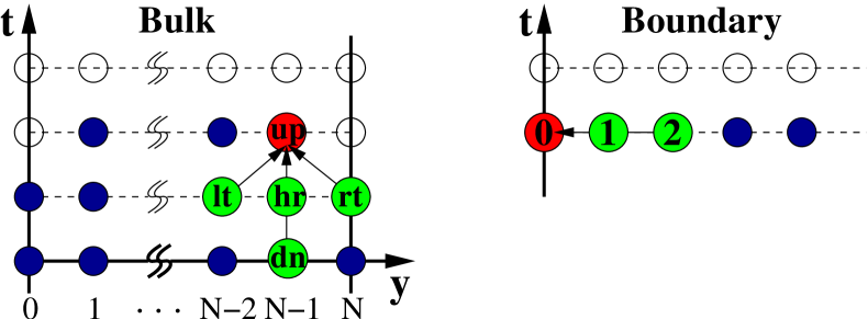
Figure 1: Numerical evolution scheme.

3.2 Boundary Conditions

The numerical scheme described in the previous subsection allows us to determine the value of the metric coefficients and of the scalar field at the next time-step for all the bulk sites, but not for the two sites $i=0,N\,$, corresponding to the positions of the two branes. To obtain the latter, the boundary conditions (2) have to be used. First we advance all the bulk sites as described in the previous section. Once we know the value of $A$, $B$, and $\phi$ in the bulk at time $t+dt$, equations (2) can be finite-differenced into a set of algebraic equations for the boundary values at that time. In the following we describe how to implement this procedure at $y=0\,$. The computation for the other brane proceeds analogously.

The boundary conditions contain first derivatives with respect to $y$ of the metric coefficients and of the scalar field at the brane locations. An asymmetric discretization for the first derivative of a generic function $f\,$, which preserves second order accuracy in $\epsilon\,$, is given by

$$f^{\prime}_{0} = \frac{1}{2\,\epsilon}\left(-\,3\,f_{0}+4f_{1}-f_{2}\right)+{\rm O}\left(\epsilon^{2}\right)\,\,.$$ (12)

Since the right hand side of the first two boundary conditions coincide, we replace the first of them simply by $A^{\prime}_{0}-B^{\prime}_{0}=0\,$, or, using equation (12),

$$-3\left(A_{0}-B_{0}\right)+4\left(A_{1}-B_{1}\right)-\left(A_{2}-B_{2}\right)=0\,\,.$$ (13)

If we define $\beta\equiv e^{B}\,$, the second boundary condition simplifies to $(1/\beta)^{\prime}={U}_{0}\left(\phi_{0}\right)/6\,$, which can be rewritten as

$$\beta_{0}=\frac{3\,\beta_{1}\,\beta_{2}}{4\,\beta_{2}-\beta_{1}-\frac{\epsilon}{3}\,{U}_{0}\left(\phi_{0}\right)\,\beta_{1}\,\beta_{2}}\,\,.$$ (14)

Finally, the third boundary condition gives

$$4\,\phi_{1}-\phi_{2}-3\,\phi_{0}-\epsilon\,\beta_{0}\,{U}_{0}^{\prime}(\phi_{0})=0\,\,.$$ (15)

Only the values of the three functions on the brane are unknown. By substituting the value for $\beta_{0}$ given by equation (14) into equation (15), the latter becomes an equation where the only unknown quantity is $\phi_{0}\,$. For specific brane potentials ${U}_{0}\,$, this equation can be solved analytically; more generally, one can solve it numerically through some iterative method. In our algorithm, the iterative Newton’s method is employed. Finally the value of $B_{0}=\ln(\beta_{0})$ can be used in (13) to determine $A_{0}\,$.

3.3 Initial Configurations

Initial conditions are imposed by specifying the three functions and their first time derivatives on the grid sites at some initial time $t_{0}\equiv 0\,$. We denote them as $A_{0}\left(y_{i}\right)$, $\dots$, $\dot{\phi}_{0}\left(y_{i}\right)\,$, with $i$ ranging from $1$ to $N-1\,$ in the bulk ($i=0,N$ are the sites of the two branes). These functions can not be chosen arbitrarily but rather must satisfy the constraint equations (2). Once this is done a second order Runge-Kutta time step is used to “convert” the initial conditions of the form $f_{0}\left(y\right)$, $\dot{f}_{0}\left(y\right)$, into initial conditions given at the first two initial time steps $f_{0}\left(y\right)$ and $f_{0+dt}\left(y\right)$. The Runge-Kutta step is done as follows

$$f_{0+dt}\left(y\right)=f_{0}\left(y\right)+dt\left(\dot{f}_{0}\left(y\right)+\frac{1}{2}dt\,\ddot{f}_{0}\left(y\right)\right)\,\,,$$ (16)

where the second time derivatives $\ddot{f}_{0}(y)$ are replaced by the equations of motion (5). This “conversion” is needed to have the initial conditions in a form suitable for the leapfrog scheme described in Subsection 3.1.

In general, the initial time derivatives can be non-vanishing, so that one can study situations in which the geometry of the extra dimension is time-dependent already at the beginning of the numerical integration. For example, this is the case for the AdS–Schwarzschild solution we will deal with in Section 4.2. For each such case the choice of initial conditions must be consistent with the constraint equations (2). We discuss one such algorithm in Section 4.2.

A particularly interesting class of initial conditions is however the one of static warped solutions

$$ds^{2}=W(y)^{2}\left(dy^{2}-dt^{2}+e^{2Ht}d{\bf x}^{2}\right).$$ (17)

characterized by a fixed bulk geometry and maximally symmetric (de Sitter or Minkowski) branes. This metric turns to the form (3) with the identification

$$B\left(t,y\right)\rightarrow B\left(y\right)=\ln W\ ,\quad\quad\quad A\left(t,y\right)\rightarrow B\left(y\right)+H\,t\ ,$$ (18)

where $H$ is the Hubble parameter of the de Sitter brane and the bulk scalar field $\phi$ is also a function of $y$ only. Such solutions were studied with dynamical system methods in [17]. The numerical integration can be used to check their stability. Numerical errors due to the grid discretization act as small perturbations. If the initial configuration is not stable, the tiny numerical errors accumulate with time, and eventually lead to an evolution of the system. When this happens, a full numerical calculation is the only tool to study where this evolution leads to, namely whether the two branes collide, move apart to infinity, or get stabilized at a finite distance in another static but stable configuration. As we will see below, in many cases de Sitter branes turn out to be unstable. Therefore even static warped geometry configurations can provide suitable initial conditions for time-dependent braneworld dynamics!

When numerical inaccuracy is used to seed the evolution, as described above, the initial amplitude and consequently the timing of the instability depends on the accuracy of the numerical integrator. This accuracy is in turn related to the spacing of the grid sites in the bulk. Increasing the number of grid sites decreases their separation, and the instability develops later. Alternatively, initial perturbations on the top of the static configurations can be imposed directly as initial conditions. This allows a quicker development of the instability, or, for static configurations, the excitation of some of the lowest eigenmodes of the system. A simple class of initial perturbations, which can be implemented in our numerical algorithm, is described in Appendix B.1 and illustrated in Figure 5. We found, however, that the qualitative behavior of the system did not depend on the details of how the initial perturbations are generated, whether imposed explicitly or through numerical roundoff errors. In the following, we therefore discuss instead how the static configurations are determined.

For static configurations, the bulk equations reduce to

$$\phi^{\prime\prime}+3\,B^{\prime}\,\phi^{\prime}-{\rm e}^{2B}V^{\prime}\left(\phi\right)=0\,\,,$$

$${B^{\prime}}^{2}+\frac{1}{6}\,{\rm e}^{2B}\,V\left(\phi\right)-\frac{1}{12}\,{\phi^{\prime}}^{2}=H^{2}\,\,.$$ (19)

In addition, the last two of the boundary conditions (2) have to be satisfied at each brane. In the gauge we are using here the constraint equations (2) are automatically satisfied.

The bulk equations are thus reduced to a system of first order differential equations for the functions $B\,,\phi\,$, and $\phi^{\prime}\,$, so that the phase space of possible solutions is effectively three-dimensional [17]. To solve these equations subject to (given) boundary conditions, we specify the values of the three functions at $y=0\,$, as well as the value of the constant parameter $H\,$. For a given brane potential $U_{0}\,$, only two of these four numbers can be chosen arbitrarily, and the other two are determined by the junction conditions at the first brane. (In the 3d phase space this means that the junction condition at the first brane defines a 1d curve in phase space along which the trajectory must begin.) The bulk equations (3.3) are then integrated with a standard fourth order Runge-Kutta integrator. Depending on the initial values and on the bulk potential, the bulk solution may become singular before the brane at $y=1$ is encountered. If this happens, some other initial values (or some other bulk potential) have to be considered.

Even if the brane at $y=1\,$ is reached, we face the nontrivial problem of satisfying the boundary conditions also at the second brane. The simplest way to solve it is to regard the junction conditions as equations for the parameters of the brane potentials. One can freely choose the three numerical values at the first brane (as well as the numerical value of $H$), integrate the bulk equations, and then use the junction conditions to determine the potentials at the two branes.  However, one is typically interested in the more difficult situations in which the brane potentials are specified, and the initial configurations have to be determined accordingly.

In the second case, we face a boundary-value problem: values of the fields satisfying the boundary conditions at the first brane do not in general lead to field values that satisfy the boundary conditions at the second brane, once they are evolved across the bulk according the bulk differential equations (3.3). It is by no means guaranteed that any choices consistent with the junction conditions at both branes exist. Indeed, as discussed in [17], many potentials do not give static solutions at all, while some others typically lead to only a finite number of them. In Appendix B we discuss the numerical method (known as the “shooting” method [22]) which we employ to find these solutions.

3.4 Units

Let us inspect the dynamical equations (5), constraint equations (2), and the boundary conditions (2). While the units of the bulk scalar field are fixed by our form of the action (1), it is easy to see that these equations are invariant under the following scaling transformation

$$A\to A+S^{\prime}\,,\,\,B\to B+S\,,$$ (20)

where $S^{\prime}$ and $S$ are arbitrary real valued transformation parameters. The scalar field potentials enter the equations only in the combinations $e^{2B}\,V$ and $e^{B}\,U$. Therefore (20) can be accompanied by the transformation

$$V\to e^{-2S}\,V,\,\,\,U\to e^{-S}\,U.$$ (21)

Suppose some metric functions $A,B$ are the solutions of (5) for given potentials $V,U$. The scaling transformations (20) and (21) tell us that from these metric functions we can generate a family of solutions for re-scaled potentials. This is very useful for introducing the units of scales for numerics. Indeed, while $y$ and $t$ in (3) are 2d conformal length and time (i.e. affine parameters along corresponding directions), the metric function $e^{B}$ defines the physical interbrane distance $D$ and the physical time. As often occurs in numerical simulations, it is not always easy to extend the range of variables, like $e^{B}$ in our case. As we will see in the example of the next Section, numerical stability (without brane stabilization) has a controlled but finite life time. If we naively increase the scale of $e^{B}$, the stability will be short-lived. The trick is to continue to work with numerically convenient values of $e^{B}$, but interpret scales in units of $l=e^{S}\,l_{5}$. One can take $S$ to be large enough to have the scale $e^{S}\,l_{5}$ much greater than the fundamental bulk scale $l_{5}$. This is to say that numerically we solve our equations not only for a given scale and given choice of parameters of the potential, but for the whole family of scales and parameters which corresponds to the orbit of the group transformation (20), (21). For the parameters of the potentials (2) we have the following units: $[m]=e^{-S}M_{5}$, $[M]=e^{-S}M_{5}$, $[\Lambda]=e^{-2S}M_{5}^{5}$, $[\lambda]=e^{-S}M_{5}^{4}$, $[\phi]=[\sigma]=M_{5}^{-3/2}$.

The time evolution of variables in the paper will be plotted versus conformal time $t$. The units of $t$ are the light crossing time between branes. This corresponds to the distance between branes in the conformal coordinate $y$ which is simply $1$ in our units.

As usual, the parameters for the numerical simulations do not allow the introduction of a large hierarchy, since numerical inaccuracies accumulate much faster. Therefore most of the parameters are chosen to be of order unity in our units. The values of parameters that correspond to the numerical runs shown in the figures of this paper are collected in the Table 1 in the Appendix.

4 Branes in AdS Background Without a Scalar Field

The algorithm presented above allows an exact integration of general two-brane configurations with bulk scalar fields. In this and in the next sections we discuss in detail several applications. The first two examples of this section have no scalar field, and the evolution is known analytically. We report them mainly to discuss the accuracy of the code and to outline its main features. The code is accurate enough to reproduce the known analytic solutions. In the following sections we will study the more complicated non-linear evolution of a system with a scalar field, for which the solutions were not previously known. Fortunately, we still will be able to check certain properties of the solutions analytically.

In this section we first consider the static unstabilized Randall-Sundrum flat brane solution, from the point of view of the numerical solution of the equations. Then we study non-static (moving) branes in an AdS-Schwarzschild background, and compare the numerical solution with the known AdS-Schwarzschild solution.

4.1 The Randall–Sundrum Model

Our first example is the two-brane Randall-Sundrum model [5]. It represents a particularly simple example of a brane world that only consists of a five dimensional AdS space with a curvature radius $l^{2}=-6/\Lambda$, determined by its 5d cosmological constant $\Lambda$, and of two flat branes with tensions $\lambda_{i}=\pm 6/l$ . The system is entirely described by one time independent function. In terms of the 2d conformal gauge (3) we have

$$A\left(y\right)=B\left(y\right)=-\ln\left[\frac{y+\left({\rm e}^{D/l}-1\right)^{-1}}{l}\right]\,\,,$$ (22)

where $D\,$ can take any constant value, which - according to equation (4) - corresponds to the interbrane distance.

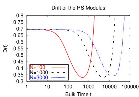
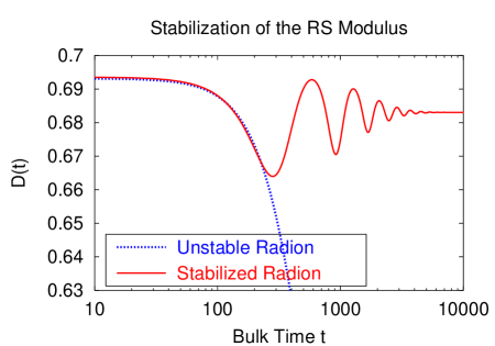
Figure 2: Left Panel: Drift of the free modulus of the RS model depending on the numerical accuracy. Right Panel: Stabilization of the RS radion.

We can reproduce this set-up in our code by simply setting to zero all the scalar field related parameters in the bulk/brane potentials in equations (5) (as well as the initial conditions for the scalar field). The numerical solutions of the equations (5) are in agreement with (22). As discussed in section 3.3, small perturbations are unavoidably introduced by the discretization. Thus, this set-up is particularly useful for verifying the accuracy of the code. Notice also, that numerical instability is much worse for the RS without stabilization. In the left panel of Figure 2 we show how the time-scale at which the instability develops is related to the number $N$ of bulk sites. The more we increase $N$ the more the accuracy of the computation increases, and numerical instability is delayed for the later times. We estimate the time scale where the code is stable as being proportional to the grid resolution $N$.

The right panel of Figure 2 also shows how the introduction of the stabilization mechanism (with the bulk scalar fields with the potential (2)) can, for appropriate choices of the parameters, lead to a stabilization of the interbrane distance. In this his case the code is much more stable. We discuss this issue in more detail in Section 5.

The choice of parameters and initial conditions that was used in the numerical runs plotted in Figure 2 as well as the ones for all following simulations are collected in Table 1.

4.2 The AdS–Schwarzschild Solution

Starting from a setting similar to the Randall-Sundrum example of the previous section, but allowing for non-vanishing initial (at $t=t_{0}$) time derivatives, we generate time-dependent numerical solutions that belong to a larger class of solutions. Assuming the initial spatial profile $A\left(t_{0},y\right)=B\left(t_{0},y\right)$ of equation (22), the constraint equations (2) are solved by

$$\dot{A}(t_{0})=c\,\left[y+\frac{1}{{\rm e}^{D/l}-1}\right]\quad,\quad\quad\dot{B}(t_{0})=-\dot{A}(t_{0})\,\,,$$ (23)

where $c$ is a constant. The choice $c=0$ gives Randall-Sundrum solutions, while a non-vanishing $c$ corresponds to moving branes. From the Birkhoff theorem for plane-parallel brane configurations it follows [19] that the generic 5d bulk metric must be a stripe of the AdS–Schwarzschild geometry (where the Schwarzschild mass is virtual because it is screened by the branes). Thus, the branes are moving in an AdS–Schwarzschild background. To see this, note that in the absence of the scalar field and for brane tensions as in the Randall-Sundrum model, the boundary conditions (2) give $A^{\prime}\left(A^{\prime}+B^{\prime}\right)=2\,\Lambda\,{\rm exp}\left(2\,B\right)\,$ at the location of the two branes. From the bulk equations, we then recover

$$\ddot{A}+2\,\dot{A}^{2}-\dot{A}\,\dot{B}=0\quad,\quad\quad y=0,\,1\,\,,$$ (24)

which, in terms on the proper time $\tau$ and the Hubble parameter $H_{i}$ on the two branes (cf. equations (9) and (10)), becomes

$$\frac{d\,H_{i}}{d\tau}+2\,H_{i}^{2}=0\,\,.$$ (25)

This corresponds to a radiation dominated standard four dimensional Universe,

$$H=\frac{H_{0}}{1+2\,H_{0}\,\left(\tau-\tau_{0}\right)}\,\,.$$ (26)

The appearance of effective radiation domination on the branes is characteristic of an AdS–Schwarzschild bulk geometry [18]. The invariant of the 5d Weyl tensor $C^{2}=C_{ABCD}C^{ABCD}$ projected into the brane scales as $C^{2}\propto a^{-8}\,$, where $a\left(\tau\right)\,$ is the scale factor of the induced FRW brane metric. Since $a\left(\tau\right)\,$ is radiation dominated, at the brane we have

$$C^{2}=C_{0}^{2}\left[1+2\,H_{0}\left(\tau-\tau_{0}\right)\right]^{-4}\,\,.$$ (27)

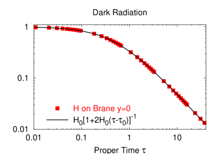
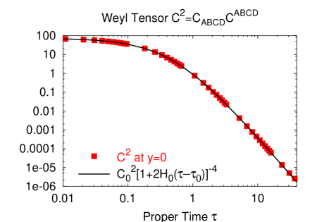
Figure 3: Comparison between numeric and analytic solutions for the Hubble parameter and Weyl tensor on the brane.

The two equations (26) and (27) are independent of the choice of coordinates in the bulk, and can be easily reproduced with our code. For a particular realization of the initial conditions (23) with the parameter $c=1$, in Figure 3 we plot the numerical calculation (squares) of the time evolution of $H$ and the 5d Weyl tensor on the brane. Solid curves correspond to the AdS-Schwarzschild analytic solutions (26) and (27). The agreement between numerics and analytics is manifest.

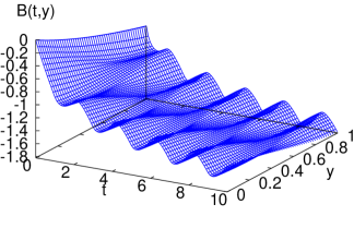
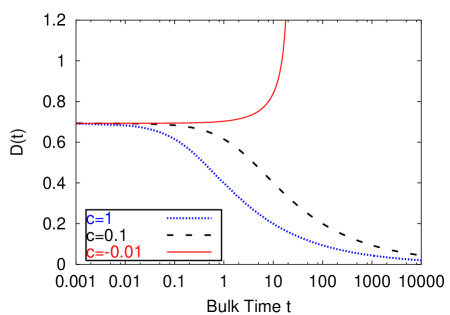
Figure 4: Left panel: Non-physical waves appearing as gauge modes in the metric function $B\left(t,\,y\right)$ (for $c=1$). Right panel: interbrane distance for various initial conditions controlled by the parameter $c$.

In the left panel of Figure 4, we show instead the evolution of the metric component $B\left(t,\,y\right)$ for the same configuration used to generate Figure 3. The ripples of $B(t,\,y)$ are not physical. As mentioned in Section 2, our choice of coordinates does not fix the gauge completely. The residual gauge freedom appears numerically as ripples in $B(t,\,y)$. The precise form of these gauges modes is worked out in Appendix A.2, and is in agreement with the numerical plots. The lowest frequency mode of these gauge modes generically appears in the evolution of $B\left(t,\,y\right)\,$. In the left panel of Figure 4, we see this effect in the form of two bulk waves with period $2\,$, which propagate on top of the profile of $B\left(t,\,y\right)$. As discussed in Section 2, these gauge modes do not affect the interbrane distance, as defined in equation (4).

The numerical evolution of the interbrane distance for the AdS – Schwarzschild solution is shown in the right panel of Figure 4 for different values and signs of the parameter $c\,$. For positive $c$ the branes approach each other, while for negative $c$ they move apart.

5 Instability of de Sitter Branes and Restructuring of Warped Configurations

Let us now study the evolution of the system (5) in the presence of a bulk scalar field. We have to specify initial conditions, which do satisfy the constraint equations. This task is now more complicated than it was without the scalar field.

5.1 Instability of Warped Geometry with Curved Branes

As a starting point we can check the code for known static warped geometry configurations (18) with the scalar field and potentials chosen so as to stabilize the branes. We can then impose perturbations consistent with the constraint equations. (This technique is described in detail in the Appendix  B.1)

Static solutions of warped geometries with bulk scalar fields and with branes at the boundaries have been studied and classified in [17]. In the 2d conformal gauge the static solutions with curved branes are given by

$$A(y,t)=B(y)+H\,t\,\,\,,\phi=\phi(y),$$ (28)

where $B(y)$ and $\phi(y)$ are related through a set of ordinary differential equations, which can be treated with the methods of [17].

We use scalar field potentials (2), which are designed for brane stabilization. The outputs of numerical integration of an initially static configuration of two curved (de Sitter) branes and bulk scalar filed with small perturbations around it is shown in Figure 5.

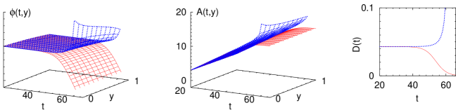
Figure 5: Instability of static solutions with dS branes: Perturbations have induced significant departure from the static solution at $t\approx 40$. The two unstable solutions shown correspond to positive (blue, upper surfaces and increasing $D$) and negative (red, lower surfaces and collapsing $D$) initial perturbations of $\delta\phi$, see Appendix B.1.

We see the appearance of time-dependence in the initially static field $\phi(y)$, departure of metric function $A$ from the hypersurface described by equation $A(y,t)=B(y)+H\,t$, and a change in the interbrane distance $D$. We show two realizations of this model with different initial perturbations. From these results we conclude that, surprisingly, the static solutions with scalar field potentials that are supposed to stabilize branes are unstable for a range of $H$!

Fortunately, this unexpected result, which we found here numerically, can be independently obtained with analytical methods reported in the accompanying paper [16]. Indeed, it is possible to consider linearized perturbations of the bulk scalar field $\delta\phi$ and scalar metric perturbations

$$ds^{2}=W(y)^{2}\left[(1+2\Phi)dy^{2}+(1+2\Psi)\left(-dt^{2}+e^{2Ht}d{\bf x}^{2}\right)\right].$$ (29)

around the background warped geometry (17), where $\Phi$ and $\Psi$ are small metric perturbations. From the linearized Einstein equations one can derive second order differential equations for the fluctuations, which can be factorized into 4d massive scalar harmonics on the de Sitter slices and KK eigenfunctions with eigenvalues $m$. The lowest eigenvalue in the KK spectrum corresponds to the radion mass. The lowest eigenvalue $m^{2}$ is estimated as

$$m^{2}=-4H^{2}+m_{0}^{2}(H)\ ,$$ (30)

where $m_{0}=\frac{2}{3}\,\frac{\int\,dy\,{\rm e}^{-B}}{\int\,dy\,{\rm e}^{-B}{\phi^{\prime}}^{-2}}$ is a functional of $H$. In many cases the first (negative) term in (43) exceeds the second positive term, causing a tachyonic instability of the curved branes. Indeed, the temporal part of the eigenmodes has an exponential instability

$$f_{m}(t)\propto e^{\mu\,t},$$ (31)

where

$$\mu=\left({\sqrt{\frac{9}{4}+\frac{|m^{2}|}{H^{2}}}-\frac{3}{2}}\right)\,H.$$ (32)

The time dependence from numerical calculations corresponding to Figure 5 is consistent with the analytic result (31). In the limit of $H=0$ formula (30) is reduced to the known result for flat branes where the branes configuration is stable [15]. The curvature of the branes upsets the balance between the bulk scalar gradients and its potentials, which otherwise provide stabilization.

Thus, both from numerics and analytics we conclude that many static configurations with de Sitter branes are unstable against classical (or quantum) fluctuations. While in the following we mostly discuss the physical meaning and consequences of this result, here we also note that this effect provides us with a tool to study brane dynamics numerically. This is because we can start with a simple controllable static configuration, without needing to resolve the time-dependent constraint equations. Doing so, we can investigate numerically fully non-linear time dependent dynamics due to the real physical tachyonic instability of the initial configuration.

Depending on the sign of the initial perturbations (the coefficient $\rho$ in equation (66)) we encounter runaway behavior towards smaller or larger interbrane distances as shown in Figure 5. We consider this type of non-linear dynamics in Section 6. Sometimes we do not find a runaway behavior, but rather a re-structuring of brane configurations as a transition between (at least) two static warped geometries. This case will be considered in the next subsection.

5.2 Dynamical Transition between Two Static Solutions

As we discussed in the Introduction, the construction of brane models with de Sitter branes is particularly challenging. Stable static solutions with inflating branes can only be achieved provided the spatial gradient of the bulk scalar field is sufficiently high, cf. equation (30).

In the context of static warped geometries, brane embeddings can be investigated in geometrical terms in a three dimensional phase space [17]. This technique is especially useful to show that more than one static solution for a given brane model, i.e. given potentials $V(\phi)$ and $U_{i}(\phi)$, might exist as illustrated in Figure 10. Many of these solutions are unstable, as shown above. A fully numerical integration is a powerful (and maybe the only) tool to study the non-linear dynamics of the unstable brane configurations. A more comprehensive study of this issue, with different bulk/brane potentials taken into account, will be presented elsewhere. Here we limit our discussion to potentials of the class (2). In this subsection we discuss the case in which the braneworld model admits one unstable and one stable static solution, and the evolution of the system drives a transition between the two. Small perturbations around the unstable solution trigger the tachyonic instability of the system, which is followed by a rapid evolution of the bulk configuration.

An example of dynamical transition between two static brane configurations is shown in Figure 6. We plot the time evolution of the distance $D(t)$ between the branes, the radion mass $m^{2}$, the Hubble parameter (curvature) $H$, and the Weyl tensor invariant $C^{2}$. The last two are defined as the averages of these quantities over the extra dimension. We observe a transition between two states, from an initial brane configuration with higher brane curvature (larger $H$) to a final configuration with lower curvature (smaller $H$). The first state is unstable; during this regime the radion mass is tachyonic, $m^{2}<0$. The value $H$ decreases with time until the second term in (43) dominates and the tachyonic instability ceases. In the cases we have studied, the decrease of $H$ is accompanied by a decrease of the physical interbrane distance, until the stable configuration is reached.  The final static configuration has positive $m^{2}$.

The dynamics of the transition between the two static configurations is quite violent, and is accompanied by a burst of the Weyl tensor $C^{2}\,$. The value of $C^{2}$ vanishes for the warped geometry configurations at the beginning and the end of the transition.

Remember that we restrict ourselves to $(t,y)$ dependence and “planar” symmetry of the metric. Of course, the actual dynamics between two warped configurations does not necessarily occur in this class of metrics, and 3d inhomogeneities along the brane can be excited. As shown in [16], the tachyonic instability of warped geometry with de Sitter branes occurs for scalar long-wavelength inhomogeneous modes with 3d momenta ${\bf k}$. The present form of the BraneCode cannot take them into account. We assume that the background ${\bf k}\to 0$ mode dominates, but this should be investigated in the future. Tensor inhomogeneous modes do not have tachyonic KK spectra [24] around the curved brane warped geometry. In fact, gravitational waves are absent for systems with planar symmetry. However, based on the evolution of the Weyl tensor $C^{2}$, we conjecture that the actual dynamics is accompanied by a burst of gravitational wave emission with 3d momenta of the order of the non-adiabatic frequency $\sim 1/\Delta t$, where $\Delta t$ is the time of transition. It will be interesting to check this with a linear tensor mode analysis around the background geometry of the Figure 6.

It is interesting to follow how the final state of the unstable warped configuration depends on the parameters of the potentials. We illustrate this with the parameter $M$ of the potential (2). In the example shown, the four dimensional cosmological evolution on the two branes is characterized by a transition between two de Sitter spaces. In the right panel of Figure 6 we show how the four dimensional Hubble parameter on one of the two branes changes as we change the brane mass parameter $M$ of the scalar field, while leaving the other parameters unchanged. In the limit of large $M$, the value of the scalar field on the branes is always very close to its expectation value $\sigma\,$. Moreover, phase space portraits [17] (see Appendix B) indicate that the two static configurations approach each other in this limit. This is also visible in Figure 6, where we see that the difference between the initial and the final value of $H$ decreases as $M$ is increased. As an analogy, one may say that higher mass parameters $M$ correspond to more rigid systems, characterized by stiffer and quicker transitions between the two static regimes. Tuning the parameters of the model, one can have flat Minkowski branes in the stable final configuration.

In the limit of negligible $M$ the system does not admit stable configurations at all. The curve with $M=1\,$, shown in Figure 6, corresponds to a case in which the dynamics of the system lead to a collision between the two branes. This case is discussed in detail in the next section.

6 Brane Collisions

Unstable warped configurations of curved (de Sitter) branes provide suitable initial conditions for studying colliding branes, as we saw in Subsection 5.1. By controlling the initial fluctuations (see Figure 5) we can generate numerical runs with brane collisions.

The collision of branes is an interesting subject by itself. In cosmology colliding branes appear in models of brane inflation [6] as well as in models without (early universe) inflation [25]. The latter models have difficulties which were discussed elsewhere (see e.g. [26]). In this paper, we focus on the issue of the bulk geometry and scalar field profiles of colliding brane configurations, in a more general context.

In the next Subsection  6.1 we show a numerical example of the brane collision and try to understand the properties of the interbrane geometry. We find that they become independent of the specific brane/bulk potentials of the model. In Subsection  6.2 we further argue that there is a universal Kasner-like space-time asymptotic of the interbrane geometry. This is a strong-gravity regime which can not be described in 4d by the moduli approximation.

6.1 Geometry Between Branes

Figure 7 and Figure 8 show in detail the evolution of the bulk scalar field $\phi(t,y)$, metric functions $A(t,y)$, $B(t,y)$ and interbrane distance $D(t)$ in runs which begin with an unstable warped de Sitter brane configuration and end with a brane collision.

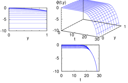
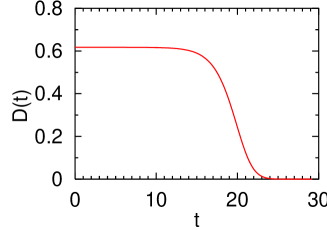
Figure 7: Flattening of $\phi$ gradients during the brane collision. The left panel shows $\phi(y)$ for different $t$, going from top to bottom. The lower panel shows $\phi(t)$ different $y$. In either plot you can see that $\phi$ becomes nearly homogeneous at later times.

The first thing to notice is that the system becomes homogeneous along the $y$ coordinate. This is seen as the flattening of $\phi$ gradients over time. A similar flattening in $y$ direction occurs for the metric components, see Figure 8. Also notice that the absolute value of $\phi$ increases with time. This increase can be fit well by $\phi(t)\sim\ln t$.

A second feature of the brane collision is the decrease of the metric component $e^{B}\,$; asymptotically $B\rightarrow-\infty$ during the collision, cf. the definition (4) of the interbrane distance. Recall that the bulk/brane scalar field potentials in the bulk equations (5) and boundary conditions (2) are always multiplied by exponents $e^{B}$. Therefore the contribution of the bulk/brane potentials becomes more and more negligible in the dynamical equations (5) during the collision.

This leads us to the important conclusion that asymptotically the dynamics of the brane collision do not depend on the form of the bulk/brane potentials. Notice, however, a potential exclusion from this rule related to exponential potentials $e^{\alpha\phi}$. In this case the typical logarithmic time divergence of $\phi$ leading up to the collision leads to the growth of the value of the potentials with time which may compensate the decrease of the metric function $e^{B}\,$. In this paper we concentrate on the potentials (2) where asymptotically the dynamics are potential-free.

This potential-free asymptotic immediately helps to explain heuristically the first feature, why the system becomes homogeneous along the $y$ coordinate. Indeed, looking at the boundary conditions, we see that the gradients of $A\,$, $B\,$, and $\phi\,$ at the branes are proportional to $\exp(B)$ and therefore vanish as $e^{B}\to 0$.

Next, let us consider equations (5) under the assumption that the bulk/brane potentials for the scalar field can be neglected and that the geometry becomes homogeneous. After this simplification equations (5) become ordinary differential equations, which can be easily solved. We find

$$A = A_{0}+\frac{1}{3}\,{\rm ln}\left(t_{c}-t\right)\,\,,$$

$$\phi = \phi_{0}-r\,{\rm ln}\left(t_{c}-t\right)\,\,,$$

$$B = B_{0}-\frac{1}{3}\left(1-3\dot{B}_{0}t_{c}-\tfrac{3}{2}r^{2}\right)\frac{t}{t_{c}}-\frac{1}{3}\left(1-\tfrac{3}{2}r^{2}\right)\,{\rm ln}\left(t_{c}-t\right)\ .$$ (34)

The constants of integration $A_{0},B_{0},\phi_{0}$ correspond to the values of the fields at some time $t=0$. The time $t=0$ cannot be the beginning of integration where we know that the approximation does not hold. We will give meaning to the integration constants shortly. The collision time is $t_{c}=-1/\dot{A}_{0}$. We also introduce a convenient intermediate parameter $r=\dot{\phi}_{0}\,t_{c}$. The brane collision corresponds to values of $r$ satisfying $r^{2}\leq\frac{2}{3}$. The scalar field potentials, as well as inhomogeneities along the $y$ coordinate, result in small corrections which are neglected in (6.1). Asymptotically the logarithmic terms in (6.1) dominate and we arrive at a homogeneous metric with power-law dependence on time. This is nothing but the recognizable Kasner-like space-time metric.

6.2 Universal Kasner-like Asymptotic

The regime when the logarithmic terms in (6.1) determine the behavior of the system corresponds to the universal Kasner solution in five dimensions with a massless scalar field. Four dimensional homogeneous but anisotropic Kasner solutions with the massless scalar field were constructed a long time ago in [27]. Its higher dimensional generalization is obvious [28]. Indeed, in 5d we have the following exact solution with the massless scalar field

$$ds^{2} =-d\tau^{2}+\tau^{2p_{\text{y}}}dy^{2}+\sum\limits_{i=1}^{3}\tau^{2p_{i}}dx_{i}^{2}\,\,,$$

$$p_{1}+p_{2}+p_{3}+p_{\text{y}} =1$$

$$p_{1}^{2}+p_{2}^{2}+p_{3}^{2}+p_{\text{y}}^{2} =1-q^{2}$$

$$\phi =q\ln\tau\,\ .$$ (35)

The vacuum Kasner solution has $q=0$. The parameter $q$ characterizes the contribution of the scalar field. The time $t$ in the 2d conformal gauge (3) and $\tau$ are related by transformation

$$t=\tau^{1-p_{\text{y}}}.$$ (36)

The significance of the Kasner-like space-time (6.2) is not only in the fact that it is an exact solution of the Einstein equations, but mostly because it is a generic asymptotic of arbitrary collapsing solutions [29].

In this section we explicitly demonstrate how the geometry of colliding branes, as a case of the collapsing solution, approach the universal Kasner-like asymptotic.

Kasner-like geometry as generic collapsing solution was already advocated in string cosmology [30]. As we show here, this asymptotic also applies to brane cosmology (in other words string cosmology with branes). There is, however, a specific new feature that appears in the brane cosmology case. The isometry in the brane directions is reflected in the additional constraint. In 5d

$$p_{1}=p_{2}=p_{3}\ .$$ (37)

This constraint and the two equalities for Kasner indices allow to express $p_{1}$ and ${p_{\text{y}}}$ through the parameter $q$

$$p_{1}=\frac{1}{4}\left(1\pm\sqrt{1-\frac{4}{3}q^{2}}\right)\,,\hskip 10.00002pt{p_{\text{y}}}=\frac{1}{4}\left(1\mp 3\sqrt{1-\frac{4}{3}q^{2}}\right)\,.$$ (38)

The range of the parameter $q$ is $-\frac{\sqrt{3}}{2}\leq q\leq\frac{\sqrt{3}}{2}$; the range of $p_{y}$ and $p_{1}$ correspondingly are $-\frac{1}{2}\leq p_{y}\leq 1$ and $0\leq p_{1}\leq\frac{1}{2}$. In the vacuum limit of vanishing $q$ one finds $p_{1}=0$ or $1/2$ and $p_{\text{y}}=1$ or $-1/2$.

One of the feature of the Kasner-like asymptotic is a chaotic alteration of the indices $p_{A}$ [29], with alternating contraction and expansion in some of the directions. In the presence of the scalar field the process ceases as all $p_{A}$ become positive. For colliding branes $p_{y}>0$, which gives $0<p_{1}<\frac{1}{3}$, so both indices are positive and no alteration of indices is expected.

For our case (37) the Kasner solution (6.2) can be rewritten to the 2d conformal gauge with the help of the time redefinition (36)

$$ds^{2}=t^{\frac{2p_{\text{y}}}{1-p_{\text{y}}}}\left(dy^{2}-dt^{2}\right)+t^{\frac{1}{3}}d\vec{x}^{2}\,.$$ (39)

In terms of the metric functions $A$ and $B$ and the field $\phi$, the Kasner solution (39) reads as

$$A = \frac{1}{3}\ln(t_{c}-t)\ ,$$

$$B = \frac{p_{y}}{1-p_{y}}\ln(t_{c}-t)\ ,$$ (40)

$$\phi = \frac{q}{1-p_{y}}\ln(t_{c}-t)\ .$$

The solution (6.2) is identical to the leading terms of (6.1) by the identification $q=6r/(3r^{2}+4)$ Thus the integration constant $r$ in (6.1) is related to the parameters of the Kasner solution. Figure 8 shows how the metric components $A$ and $B$ and the field $\phi$ found numerically, approaches the universal Kasner asymptotic (39).

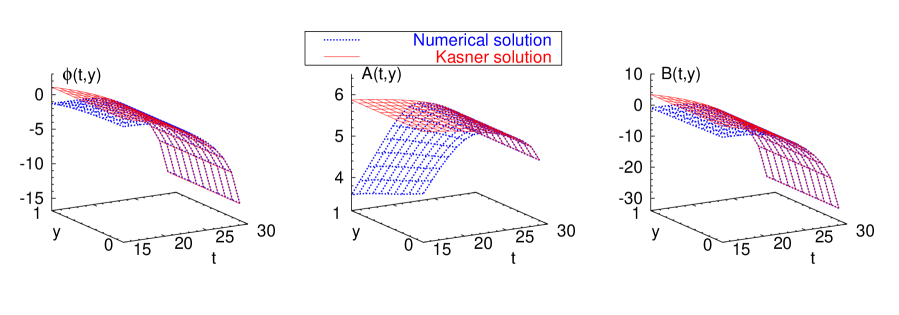
Figure 8: Numerical solutions (lower red surfaces) asymptotically approach universal Kasner-like solution (upper blue $y$ - independent surfaces).

Next, consider metrics induced by the bulk Kasner geometry at the branes (which is independent of $y$)

$$ds^{2}=-d\tau^{2}+(\tau_{c}-\tau)^{2p_{1}}d\vec{x}^{2}\ ,$$ (41)

The induced Hubble parameter on either branes is then given by

$$H=-\frac{p_{1}}{t_{c}-t}\ .$$ (42)

This time-dependence of the Hubble parameter at the brane is a good fit to the asymptotic behavior of the Hubble parameter we found numerically, as illustrated in Figure 9.

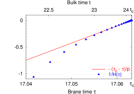
Figure 9: Induced Hubble parameter $H(\tau)$ at the colliding branes

The induced metric at the brane (41) depends on the parameter $q$ through the index $p_{1}$. This parameter is absent in the simple moduli approximation of the 4d effective theory at the brane, which does not take into account strong gravity arising in the bulk geometry.

7 Summary

We design the numerical code, BraneCode${}^{\mbox{\textregistered}}$, to treat non-linear time-dependent dynamics of 5d braneworlds with plane-parallel branes at the edge and with bulk scalar field with arbitrary bulk and brane potentials. It is possible to choose a convenient gauge where the brane positions are not changing with time, and dynamics is imprinted in two metric components and bulk scalar field. These bulk equations for gravity and the scalar field are supplemented by boundary conditions at the orbifold branes and initial conditions in the bulk. We also treat the constraint equations at the initial time hypersurface. So far we have only included a single bulk scalar field, but the code could in principle be extended to include other layers such as additional scalars in the bulk or on the branes.

We check the code for the brane models with known analytic solutions. For two branes embedded in the 5d background with negative 5d cosmological constant without the scalar field we numerically reproduce generic AdS-Schwarzschild solution

Next, we consider more comprehensive braneworlds with the bulk scalar field. We investigate numerically small perturbations around warped stationary configuration with bulk scalar and with de Sitter branes including the bulk/brane potentials, which are introduced for the brane stabilization. However, for the large enough 4d curvature of inflating branes the system is unstable and runs away from the initial warped configuration with de Sitter branes. This effect is confirmed independently by an analytic calculation of small scalar perturbations in this setting [16]. The scalar fluctuations around a warped configuration with curved branes have as their lowest eigenvalue

$$m^{2}=-4H^{2}+m_{0}^{2}(H)\ .$$ (43)

The term $m_{0}(H)$ is a functional of $H$, and depends on the parameters of the model. If parameters are such that $m^{2}$ becomes negative due to excessive curvature $\sim H^{2}$, the brane configuration becomes unstable. For relatively low values of $H^{2}$ the radion mass (43) is positive and the system is stable. Our interpretation of this instability is the following. Stabilization of flat branes is based on the balance between the gradient $\phi^{\prime}$ of the bulk scalar field and the brane potentials $U(\phi)$ which tends to keep $\phi$ pinned down to its values $\phi_{i}$ at the branes. The interplay between different forces becomes more delicate if the branes are curved, and for the brane curvature exceeding some critical value the brane configuration becomes unstable.

Tachyonic instability of curved branes has serious implications for theory of inflation in the braneworlds and is discussed in details in the accompanying paper [16].

Our numerical simulations allow us to follow dynamics of the brane configuration triggered by the tachyonic instability. The end point of evolution depends on the presence or absence of another (or others) warped stationary configurations in the model.

The question about the multiplicity of warped solutions can be studied in the framework of warped geometry with no time-dependence. We implemented the geometrical constructions in the phase space of solutions of the gravity plus scalar system that had been developed earlier. In the model with quadratic bulk and brane potentials, depending on the parameters there are single or double warped solutions.

Thus we see that in some cases the warped branes system can admit two solutions for the same parameters of the potentials, with different values of the curvature of the de Sitter brane, which is proportional to $H^{2}$. Suppose we start a numerical run with the warped solution that has a larger value of the brane curvature, which is unstable. Then we observe numerically that this configuration evolves dynamically and ends up in the the state which corresponds to the second warped solution. The second solution is stable if the corresponding radion mass $m^{2}$ is positive, as in the example shown in the text. This re-structuring is accompanied by strong dynamical features like a burst in the Weyl tensor, which vanishes in the initial and final warped configurations. Although inhomogeneous tensor modes are not included in the code, based on this behaviour of the Weyl tensor we conjecture that brane re-structuring should be accompanied by the emission of gravitational waves due to the non-adiabaticity of the process.

All together, this process looks like a decay of the meta-stable state of the strongly curved branes due to the tachyonic instability into the more stable state where the branes have lower curvature. This transition is marked by a burst of gravitational field anisotropy (gravitational waves?). It will be interesting to investigate what applications this may have to cosmology with branes. Another potential application of brane restructuring would be the problem of the 4d cosmological constant in the braneworld picture. The cosmological constant problem was discussed recently from a braneworld perspective, in which a low 4d cosmological constant corresponds to a flat brane. There was a suggestion that the flat brane is a special solution of the bulk gravity/dilaton system with a single brane [32], but the model has difficulties [33]. In our setup, we consider two branes. The new element which emerges from our paper is the instability of the curved branes. So far we have only shown an example of re-structuring between two curved brane configurations. It will be interesting to see if there are brane models with more than two stationary warped geometry configurations, or with several scalar fields, and to investigate if there is a mechanism for brane flattening.

Finally, we studied the geometry of colliding branes. As initial conditions we used the unstable curved brane configurations with parameters which do not allow another warped geometry configuration. In such cases the end point of the brane dynamics is either a brane collision or branes moving apart. We investigated in detail the geometry of colliding branes. The bulk metric and the bulk scalar field become homogeneous, i.e. $y$-independent, and the brane dynamics asymptotically does not depend on the scalar field potentials. Instead, the geometry of colliding branes asymptotically approaches a universal Kasner-like solution with a free scalar field. It is known that the Kasner asymptotic is a generic solution of the high dimensional gravity/dilaton system [30]. In our case isometry of the brane slices guarantees equality of the Kasner indices $p_{1}=p_{2}=p_{3}$. In 5d this condition leaves only one single parameter of the Kasner-like solution $q$, associated with the bulk scalar field contribution. This parameter is determined by the initial conditions. For the 5d brane system we considered, there is no chaos in the alteration of the Kasner indices. It will be interesting to investigate this issue for other situations, for example when the form field is included and the brane dimensions and co-dimensions are different.

Appendices

Appendix A Choice of Gauge

The system we are studying has a gauge freedom which amounts to different possible coordinates for the five dimensional metric and for the positions of the two branes. Our choice not only aims at simplifying the equation of motions, but also at removing “redundant” degrees of freedom which would not allow us to write a closed system of equations for the numerical integration. In Section 2, we claimed that it is always possible to choose a system of coordinates in which the $(t,y)-$part of the metric is conformally flat and in which the two branes are fixed at the positions $y=0$ and $y=1\,$, irrespective whether their physical separation is constant or changing in time. We show this explicitly in Subsection A.1. This choice does not fix the gauge completely, however. The form of the remaining gauge degrees of freedom, which are expected to affect the numerical solutions, is worked out in Subsection A.2.

A.1 Comoving Branes

By assumption, the system is homogeneous and isotropic along the spatial coordinates ${\bf x}\,$, and the position of each brane in the extra space is specified by a function of time only (parallel branes). Since the metric coefficients depend only on the two coordinates $t$ and $y\,$, the metric can be written in the 2d conformal gauge (3)

The change of coordinates

$$t \rightarrow {\bar{t}}=\frac{f\left(t+y\right)+g\left(t-y\right)}{2}\,\,,$$

$$y \rightarrow {\bar{y}}=\frac{f\left(t+y\right)-g\left(t-y\right)}{2}\,\,,$$ (44)

where $f$ and $g$ are two arbitrary scalar functions, preserves the 2d conformal gauge, since it affects the metric (3) only by the change

$$B\left(t,y\right)\rightarrow{\bar{B}}\left({\bar{t}},{\bar{y}}\right)=\left[B\left(t,y\right)-\frac{1}{2}{\rm ln}\left(f^{\prime}\left(t+y\right)g^{\prime}\left(t-y\right)\right)\right]_{t,y\rightarrow{\bar{t}},{\bar{y}}}\ .$$ (45)

This is most easily seen in null coordinates, where

$$t=\frac{v+u}{\sqrt{2}}\,\,,\,\,y=\frac{v-u}{\sqrt{2}}\;\;\Rightarrow\;\;ds^{2}=-2\,du\,dv\,\,.$$ (46)

Generally, the two branes will have a time dependent position in the extra dimension, described by the two functions $y_{1}\left(t\right)$ and $y_{2}\left(t\right)\,$, respectively. However, as long as their motion occurs slower than the speed of light, $|\dot{y}_{1}|$ and $|\dot{y}_{2}|<1\,$, we can perform a change of coordinates (44) to have them at fixed position along $y\,$, as we now show.

Let us first fix the first brane at $y\equiv 0\,$. For this to happen, the two functions $f$ and $g$ appearing in equations (44) have to satisfy

$$f\left(t+y_{1}\left(t\right)\right)=g\left(t-y_{1}\left(t\right)\right)\,\,.$$ (47)

We can choose $f$ arbitrarily, and use (47) to determine $g\,$. The condition $|\dot{y}_{1}|<1$ guarantees this can be always done, since the arguments of both the two functions increase monotonically in time.

In the new coordinate system, the first brane is fixed at $y_{1}\equiv 0\,$, while again the second one will be generally moving according to some function ${\tilde{y}}_{2}\left(t\right)\,$. This function describes the parallel motion of the second brane with respect to the first one. Since in the old system of coordinates the relative motion was at a speed lower than that of light, this will be the case also in the new coordinates, $|\dot{\tilde{y}}_{2}|<1\,$. To preserve the first brane at the origin, the residual freedom (44) is restricted to $f\left(w\right)=g\left(w\right)\,$, i.e. $f$ and $g$ are the same functions of their arguments. If we choose $f$ to satisfy

$$f\left(t+{\tilde{y}}_{2}\left(t\right)\right)=f\left(t-{\tilde{y}}_{2}\left(t\right)\right)+2\,\,,$$ (48)

we finally reach a third system of coordinates where the two branes are fixed at $y_{1}\equiv 0$ and $y_{2}\equiv 1\,$, respectively. As before, the function $f$ can always be constructed. Since $|\dot{\tilde{y}}_{2}|<1\,$, the arguments of both terms increase monotonically in time. We can then use the value of $f$ at the right hand side of equation (48) to “construct” the value of $f$ at the left hand side.

A.2 Residual Gauge Freedom

Even with the position of the branes fixed, the freedom of reparametrization is not exhausted yet. The residual gauge degrees of freedom are again of the form (44), with

$$f\left(w\right)=g\left(w\right)\equiv F\left(w\right)\quad\quad,\quad F\left(w+2\right)-F\left(w\right)=2\,\,.$$ (49)

The most generic function $F$ with this property is

$$F(w)=w+\sum\limits_{n=0}^{\infty}\left(a_{n}\cos n\pi w+b_{n}\sin n\pi w\right)\,\,,$$ (50)

with arbitrary coefficients $a_{n},b_{n}\,$. The appearance of these gauge degrees of freedom is manifest in some of the numerical results we obtained, for example in Figure 4 they are shown as ripples in the metric component $B(t,y)$.

A.3 Perturbations of the Randall-Sundrum geometry

It is interesting to note that, apart from pure gauge modes described in the previous appendix, there exists only one kind of ${\bf x}-$independent small fluctuations about the Randall-Sundrum geometry (22). As we show now, this perturbation is related to a small change of the interbrane distance $D\,$, which is not stabilized without a scalar field. We know that any ${\bf x}-$independent configuration can be written in the conformal gauge with the position of the branes at $y=0,1\,$. Thus, all the perturbations we are interested in can be written in terms of the metric components $A\left(t,y\right)=A_{0}(y)+\delta a\left(t,y\right)\,$, $B\left(t,y\right)=B_{0}(y)+\delta b\left(t,y\right)\,$, where $A_{0}=B_{0}$ is the Randall–Sundrum solution (22). To find which perturbations are allowed, we linearize the bulk Einstein equations. The dynamical ones reduce to

$$\ddot{\delta a}-\delta a^{\prime\prime}+\frac{6\delta a^{\prime}}{y+\gamma}+\frac{8\delta b}{\left(y+\gamma\right)^{2}}=0\,\,,$$

$$\ddot{\delta b}-\delta b^{\prime\prime}-\frac{6\delta a^{\prime}}{y+\gamma}-\frac{4\delta b}{\left(y+\gamma\right)^{2}}=0\,\,,$$ (51)

while the two constraint equations are conveniently recast in the form

$$\frac{d}{dt}\left(\delta a^{\prime}+\frac{\delta b}{y+\gamma}\right) = 0\,\,,$$

$$\frac{d}{dy}\left[\left(y+\gamma\right)^{-3}\left(\delta a^{\prime}+\frac{\delta b}{y+\gamma}\right)\right] = 0\,\,.$$ (52)

Here $\gamma=\left({\rm e}^{D/l}-1\right)^{-1}\,$, cf. equation (22). The last two equations give

$$\delta a^{\prime}+\frac{\delta b}{y+\gamma}\equiv C\left(y+\gamma\right)^{3}\,\,,$$ (53)

with $C$ constant. Finally, linearizing the boundary conditions we have

$$\left(\delta a^{\prime}+\frac{\delta b}{y+\gamma}\right)_{|y=0,1}=0\quad,\quad\left(\delta b^{\prime}+\frac{\delta b}{y+\gamma}\right)_{|y=0,1}=0\,\,,$$ (54)

the first of which enforces $C=0\,$. Substituting equation (53) into the second equation of (51), we have a differential equation in terms of $\delta b$ and its derivatives only. Fourier transforming

$$\delta b=\int d\omega\,{\rm e}^{i\,\omega\,t}\,{\widetilde{\delta b}}\left(\omega,y\right)\,\,,$$ (55)

we get an ordinary differential equation which is solved by

$${\widetilde{\delta b}}=F\left[{\rm cos}\left(\omega\,z\right)-\frac{{\rm sin}\left(\omega\,z\right)}{\omega\,z}\right]+G\left[{\rm sin}\left(\omega\,z\right)+\frac{{\rm cos}\left(\omega\,z\right)}{\omega\,z}\right]\quad\quad,\quad z=y+\gamma\,\,.$$ (56)

The boundary conditions for $\delta b$ at the two branes become two equations for the two parameters $F$ and $G\,$. Non-vanishing solutions are possible only for

$$\omega=n\,\pi\quad,\quad\quad n=0,1,2,\dots\,\,.$$ (57)

For these values, the two coefficients $F$ and $G$ are related by $G=F\,{\rm tan}\,\omega\,\gamma\,$. The Fourier transform of $\delta a$ is then easily obtained from the remaining two equations

$$\delta a=\frac{1}{\omega\,z}\,\left[-F\,{\rm sin}\left(\omega\,z\right)+G\,{\rm cos}\left(\omega z\right)\right]+K\delta\left(\omega\right)\,\,,$$ (58)

where $K$ is a constant. Back in coordinate space

$$\delta a = \Sigma_{n}\frac{-\,F_{n}}{{\rm cos}\left(n\pi\gamma\right)}\,\frac{{\rm e}^{i\,n\,\pi\,t}\,{\rm sin}\left(n\,\pi\,y\right)}{n\,\pi\,\left(y+\gamma\right)}+K\,\,,$$

$$\delta b = \Sigma_{n}\frac{F_{n}}{{\rm cos}\left(n\pi\gamma\right)}\,{\rm e}^{i\,n\,\pi\,t}\left[{\rm cos}\left(n\,\pi\,y\right)-\frac{{\rm sin}\left(n\,\pi\,y\right)}{n\,\pi\,\left(y+\gamma\right)}\right]\,\,.$$ (59)

These are the most generic ${\bf x}-$independent perturbations of the Randall-Sundrum solution (22). However, most of them are pure gauge modes. Let us consider infinitesimal change of coordinates of the residual gauge discussed in Appendix A.2

$$F\left(w\right) = w+{\tilde{F}}\left(w\right)=w+\sum_{n}f_{n}{\rm e}^{i\,n\,\pi\,w}\,\,,$$

$$t \rightarrow t+\sum_{n}f_{n}{\rm e}^{i\,n\,\pi\,t}\,{\rm cos}\left(n\,\pi\,y\right)\,\,,$$

$$y \rightarrow y+\sum_{n}f_{n}{\rm e}^{i\,n\,\pi\,t}\,i\,{\rm sin}\left(n\,\pi\,y\right)\,\,.$$ (60)

Under this infinitesimal change of coordinates, the metric coefficients undergo the infinitesimal changes

$$A_{0} \rightarrow A_{0}+A_{0}^{\prime}\,\frac{{\tilde{F}\left(t+y\right)}-{\tilde{F}\left(t-y\right)}}{2}\,\,,$$

$$B_{0} \rightarrow B_{0}-B_{0}^{\prime}\,\frac{{\tilde{F}\left(t+y\right)}-{\tilde{F}\left(t-y\right)}}{2}+\frac{{\tilde{F}^{\prime}\left(t+y\right)}+{\tilde{F}^{\prime}\left(t-y\right)}}{2}\,\,.$$ (61)

By choosing

$$f_{n}=\frac{i\,F_{n}}{n\,\pi\,{\rm cos}\left(n\,\pi\,\gamma\right)}\quad\quad,\quad n=1,2,\dots\,\,,$$ (62)

we see that the perturbations (59) are equivalent to

$$A_{0}+\delta a \equiv A_{0}-\frac{F_{0}\,y}{y+\gamma}+K=A_{0}+\frac{F_{0}\,\gamma}{y+\gamma}+{\tilde{K}}\,\,$$

$$B_{0}+\delta b \equiv B_{0}+\frac{F_{0}\,\gamma}{y+\gamma}\,\,,$$ (63)

where ${\cal K}=K-F_{0}$ is also constant.

By an appropriate rescaling of the spatial ${\bf x}$ coordinates we can set $\tilde{K}$ to zero.

Appendix B Determination of Static Configurations

Here we describe the method used to determine static solutions, once the bulk and brane potentials for the scalar field are given. This is done by a numerical boundary value problem solver using the shooting method. As discussed in Section 3.3, we first deal with the two boundary conditions at the first brane. Any two of $B_{0},\,\phi_{0},\,\phi_{0}^{\prime}\,$, and $H\,$ can be chosen freely, while the other two are determined by the junction conditions at the first brane. We find it more convenient to choose the values of $B_{0}$ and $\phi_{0}^{\prime}\,$, since the latter cannot be taken arbitrarily large if we want the solutions to remain regular all across the bulk. A fourth order Runge-Kutta integrator is then employed to integrate equations (3.3) in the bulk. The aim is to find the values of $B_{0}$ and $\phi_{0}^{\prime}$ for which the solutions are regular in the $0\leq y\leq 1$ interval, and for which the boundary conditions on the second brane are also satisfied. We can recast the latter in the form

$$c_{1}\equiv B_{1}^{\prime}-\frac{1}{6}{U}_{1}\,{\rm e}^{B_{1}}=0\quad\quad,\quad c_{2}\equiv\phi^{\prime}_{1}+\frac{1}{2}\frac{d{U}_{1}}{d\phi}\,{\rm e}^{B_{1}}=0\,\,.$$ (64)

Both $c_{1}$ and $c_{2}$ are only functions of the chosen value for $B_{0}$ and $\phi_{0}^{\prime}\,$, and in general do not vanish. We use Newton’s method to find the zeros of these two functions, that is the initial configurations at the first brane for which the junction conditions at the second brane are also satisfied. In practice, for the potentials we have studied, Newton’s method does not converge globally. Fortunately, the bulk equations (3.3) can be integrated very quickly, so that we can perform a “brute force” scan in the $\left\{B_{0},\phi^{\prime}_{0}\right\}\,$ plane. We then apply Newton’s method starting only from those values which are sufficiently close to a solution, i.e. for which $c_{1}$ and $c_{2}\,$ turn out to be sufficiently close to zero.

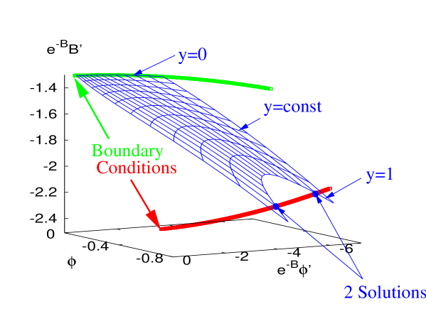
Figure 10: Phasespace illustration of the two solutions for given potentials

The existence of static solutions is not guaranteed for arbitrary bulk and brane potentials. As discussed in [17], many potentials do not give static solutions at all, while some others typically lead to a finite number of them. Using the geometrical method of phase portraits for quadratic potentials (2) we found at most two static solutions in the (wide) space of possible initial configurations we have scanned. Figure 10 shows how the phase portrait method allows us to visualize the quest for static configurations. Following the method of [17], we draw curves in the $\{\phi,e^{-B}\phi^{\prime},e^{-B}B^{\prime}\}$ phase space.

Each of the two thick curves refers to one of the two branes, and it joins points for which the junction conditions on that brane are satisfied. The thin curves are are a sampling of bulk trajectories which satisfy the junction conditions at one of the two branes (at $y=0$). Valid static solutions consist of trajectories that satisfy the junction conditions at both branes. Hence, in the phase portrait they are represented by the few trajectories which intersect both the thick curves. Lines perpendicular to the trajectories represent lines of $y=const$. We see that in the case at hand, corresponding to quadratic potentials (2), there are two intersections.

B.1 Perturbations of Static Solutions

Generic perturbations around a static configuration (18) are described by the functions $\delta B_{0}\left(y\right)$, $\delta A_{0}\left(y\right)$, $\delta\phi_{0}\left(y\right)$ and their first time derivatives $\delta\dot{B}_{0}\left(y\right)$, $\delta\dot{A}_{0}\left(y\right)$, and $\delta\dot{\phi}_{0}\left(y\right)$, which are obtained by equating the time dependent fields and the first time derivatives at an initial moment $t_{0}=0$. In the bulk, four of them can be specified arbitrarily, while the remaining functions are obtained from the constraint equations. One possible choice of initial perturbations, adopted in the example of Figure 5, is given by

$$\delta B_{0}\left(y\right) = \delta A_{0}\left(y\right)=\delta\dot{A}_{0}\left(y\right)\equiv 0\,\,,$$

$$\delta\phi_{0}\left(y\right) \equiv \delta\phi\left(y\right)\,\,,$$

$$\delta\dot{\phi}_{0}\left(y\right) = \frac{H}{A^{\prime}}\,\phi^{\prime}-\left(\frac{H^{2}}{{A^{\prime}}^{2}}{\phi^{\prime}}^{2}+\delta{\phi^{\prime}}^{2}-2\,\phi^{\prime}\,\delta\phi^{\prime}-2\,e^{2B}\left[V\left(\phi\right)-V\left(\phi-\delta\phi\right)\right]\right)^{\frac{1}{2}}\,\,,$$

$$\delta\dot{B}_{0}\left(y\right) = \frac{1}{3}\,\frac{\phi^{\prime}}{A^{\prime}}\,\delta\dot{\phi}\,\,.$$ (65)

The perturbation $\delta\phi\left(y\right)$ can be specified arbitrarily. In the example shown, the Gaussian profile

$$\delta\phi=\rho\,{\rm exp}\left(-\,\frac{\left(y-1/2\right)^{2}}{2\,h^{2}}\right)\,\,,$$ (66)

is centered between the branes. A sufficiently small values for $h$ guarantee that the perturbations are exponentially suppressed at the brane locations, leaving the junction conditions (practically) unaffected.

	Figure 2	Figure 3,4		Figure 5	Figure 6	Figure 7,8,9	Figure 10
Bulk: $V=\tfrac{1}{2}m^{2}\phi^{2}+\Lambda$	$\displaystyle m$ $\displaystyle=0$ $\displaystyle\Lambda$ $\displaystyle=-6$ $\displaystyle m$ $\displaystyle=0.5$ $\displaystyle\Lambda$ $\displaystyle=-6$	$\displaystyle m$ $\displaystyle=0$ $\displaystyle\Lambda$ $\displaystyle=-6$	$\displaystyle m$ $\displaystyle=$ $\displaystyle\Lambda$ $\displaystyle=$	$\displaystyle 0.5$ $\displaystyle-6$	$\displaystyle 0.5$ $\displaystyle-6$	$\displaystyle 0.5$ $\displaystyle-6$	$\displaystyle 1$ $\displaystyle-6$
Branes: $U_{i}=$ $\tfrac{1}{2}M_{i}(\phi-\sigma_{i})^{2}+\lambda_{i}$	$\displaystyle M_{0}$ $\displaystyle=0$ $\displaystyle\lambda_{0}$ $\displaystyle=6$ $\displaystyle M_{1}$ $\displaystyle=0$ $\displaystyle\lambda_{1}$ $\displaystyle=-6$ $\displaystyle M_{0}$ $\displaystyle=300$ $\displaystyle\lambda_{0}$ $\displaystyle=5.98$ $\displaystyle\sigma_{0}$ $\displaystyle=0.5$ $\displaystyle M_{1}$ $\displaystyle=300$ $\displaystyle\lambda_{1}$ $\displaystyle=-6.04$ $\displaystyle\sigma_{1}$ $\displaystyle=0.60$	$\displaystyle M_{i}$ $\displaystyle=0$ $\displaystyle\lambda_{0}$ $\displaystyle=6$ $\displaystyle\lambda_{1}$ $\displaystyle=-6$	$\displaystyle M_{0}$ $\displaystyle=$ $\displaystyle\lambda_{0}$ $\displaystyle=$ $\displaystyle\sigma_{0}$ $\displaystyle=$ $\displaystyle M_{1}$ $\displaystyle=$ $\displaystyle\lambda_{1}$ $\displaystyle=$ $\displaystyle\sigma_{1}$ $\displaystyle=$	$\displaystyle 2$ $\displaystyle 36.6$ $\displaystyle 0.201$ $\displaystyle 2$ $\displaystyle-49.7$ $\displaystyle-0.692$	$\displaystyle 300$ $\displaystyle 6.04$ $\displaystyle 0.000202$ $\displaystyle 300$ $\displaystyle-7.02$ $\displaystyle-0.406$	$\displaystyle 2$ $\displaystyle 6.24$ $\displaystyle 0.33$ $\displaystyle 2$ $\displaystyle-102$ $\displaystyle-1.05$	$\displaystyle 100$ $\displaystyle 7.86$ $\displaystyle 0.00815$ $\displaystyle 100$ $\displaystyle-13.9$ $\displaystyle-0.715$
Initial conditions for static solution:	$\displaystyle H$ $\displaystyle=0$ $\displaystyle\phi_{0}$ $\displaystyle=0$ $\displaystyle\phi_{0}^{\prime}$ $\displaystyle=0$ $\displaystyle B_{0}$ $\displaystyle=0$ $\displaystyle B_{0}^{\prime}$ $\displaystyle=-1$ $\displaystyle H$ $\displaystyle=10^{-4}$ $\displaystyle\phi_{0}$ $\displaystyle=0.5$ $\displaystyle\phi_{0}^{\prime}$ $\displaystyle=0$ $\displaystyle B_{0}$ $\displaystyle=0$ $\displaystyle B_{0}^{\prime}$ $\displaystyle=-0.997$	(cf. Sec. 4.2) $\displaystyle H$ $\displaystyle=0$ $\displaystyle D$ $\displaystyle=\ln 2$ $\displaystyle c$ $\displaystyle=1$ $\displaystyle\dot{A}_{0}$ $\displaystyle=y+1$ $\displaystyle\dot{B}_{0}$ $\displaystyle=-\dot{A}_{0}$	$\displaystyle H$ $\displaystyle=$ $\displaystyle\phi_{0}$ $\displaystyle=$ $\displaystyle\phi_{0}^{\prime}$ $\displaystyle=$ $\displaystyle B_{0}$ $\displaystyle=$ $\displaystyle B_{0}^{\prime}$ $\displaystyle=$	$\displaystyle 0.3$ $\displaystyle 0$ $\displaystyle-0.02$ $\displaystyle-0.3$ $\displaystyle-0.304$	$\displaystyle 0.2$ $\displaystyle 0$ $\displaystyle-0.05$ $\displaystyle 0.5$ $\displaystyle-1.66$	$\displaystyle 0.3$ $\displaystyle 0$ $\displaystyle-0.3$ $\displaystyle-0.1$ $\displaystyle-0.96$	$\displaystyle 0.0354$ $\displaystyle 0.368$ $\displaystyle-0.0508$ $\displaystyle-0.00276$ $\displaystyle-0.393$ $\displaystyle-0.241$ $\displaystyle-2.01$ $\displaystyle-0.818$ $\displaystyle-0.179$ $\displaystyle-0.579$
Mass bound:	$\displaystyle m_{\text{eff}}^{2}$ $\displaystyle=0$ $\displaystyle m_{\text{eff}}^{2}$ $\displaystyle<0.0016$	no static solution	$\displaystyle m_{\text{eff}}^{2}$ $\displaystyle<$	$\displaystyle-0.360$	$\displaystyle-0.139$	$\displaystyle 0.041$	$\displaystyle 0.17$ $\displaystyle-0.387$
Perturbations:	no	no		$\displaystyle\delta\phi$ $\displaystyle=c_{1}e^{c_{2}(y-\tfrac{1}{2})^{2}}$ $\displaystyle c_{1}$ $\displaystyle=\pm 10^{-6}$ $\displaystyle c_{2}$ $\displaystyle=-1$	no	no	no

Table 1: Parameters used for simulations presented in the figures

References

- [1] D. Langlois, Brane cosmology: An introduction, Prog. Theor. Phys. Suppl. 148, 181 (2003) [hep-th/0209261].
- [2] V. A. Rubakov and M. E. Shaposhnikov, Extra space-time dimensions: Towards a solution to the cosmological constant problem, Phys. Lett. B 125, 139 (1983).
- [3] P. Horava and E. Witten, Heterotic and type I string dynamics from eleven dimensions, Nucl. Phys. B 460, 506 (1996) [hep-th/9510209].
- [4] A. Lukas, B. A. Ovrut, K. S. Stelle and D. Waldram, Heterotic M-theory in five dimensions, Nucl. Phys. B 552, 246 (1999) [hep-th/9806051].
- [5] L. Randall and R. Sundrum, A large mass hierarchy from a small extra dimension, Phys. Rev. Lett. 83, 3370 (1999) [hep-ph/9905221]; L. Randall and R. Sundrum, An alternative to compactification, Phys. Rev. Lett. 83, 4690 (1999) [hep-th/9906064].
- [6] G. R. Dvali and S. H. Tye, Brane inflation, Phys. Lett. B 450, 72 (1999) [hep-ph/9812483]; C. P. Burgess, M. Majumdar, D. Nolte, F. Quevedo, G. Rajesh and R. J. Zhang, The inflationary brane-antibrane universe, JHEP 0107, 047 (2001) [hep-th/0105204]; C. Herdeiro, S. Hirano and R. Kallosh, String theory and hybrid inflation / acceleration, JHEP 0112, 027 (2001) [hep-th/0110271].
- [7] W. D. Goldberger and M. B. Wise, Modulus stabilization with bulk fields, Phys. Rev. Lett. 83, 4922 (1999) [hep-ph/9907447].
- [8] G. W. Gibbons, R. Kallosh and A. D. Linde, Brane world sum rules, JHEP 0101, 022 (2001) [hep-th/0011225].
- [9] H. A. Chamblin and H. S. Reall, Dynamic dilatonic domain walls, Nucl. Phys. B 562, 133 (1999) [hep-th/9903225].
- [10] J. de Boer, E. Verlinde and H. Verlinde, On the holographic renormalization group, JHEP 0008, 003 (2000) [hep-th/9912012]; A. Van Proeyen, The scalars of , and attractor equations, hep-th/0105158.
- [11] P. Kanti, I. I. Kogan, K. A. Olive and M. Pospelov, Cosmological 3-brane solutions, Phys. Lett. B 468, 31 (1999) [hep-ph/9909481]; C. Csaki, M. Graesser, L. Randall and J. Terning, Cosmology of brane models with radion stabilization, Phys. Rev. D 62, 045015 (2000) [hep-ph/9911406].
- [12] P. Binetruy, C. Deffayet and D. Langlois, Non-conventional cosmology from a brane-universe, Nucl. Phys. B 565, 269 (2000) [hep-th/9905012].
- [13] T. Shiromizu, K. i. Maeda and M. Sasaki, The Einstein equations on the 3-brane world, Phys. Rev. D 62, 024012 (2000) [gr-qc/9910076].
- [14] K. i. Maeda and D. Wands, Dilaton-gravity on the brane, Phys. Rev. D 62, 124009 (2000) [hep-th/0008188]; A. Mennim and R. A. Battye, Cosmological expansion on a dilatonic brane-world, Class. Quant. Grav. 18, 2171 (2001) [hep-th/0008192].
- [15] T. Tanaka and X. Montes, Gravity in the brane-world for two-branes model with stabilized modulus, Nucl. Phys. B 582, 259 (2000) [hep-th/0001092]; S. Mukohyama and L. Kofman, Brane gravity at low energy, Phys. Rev. D 65, 124025 (2002) [hep-th/0112115].
- [16] A. V. Frolov and L. Kofman, Can inflating braneworlds be stabilized?, hep-th/0309002.
- [17] G. N. Felder, A. V. Frolov and L. Kofman, Warped geometry of brane worlds, Class. Quant. Grav. 19, 2983 (2002) [hep-th/0112165].
- [18] P. Kraus, Dynamics of anti-de Sitter domain walls, JHEP 9912, 011 (1999) [hep-th/9910149]; P. Binetruy, C. Deffayet, U. Ellwanger and D. Langlois, Brane cosmological evolution in a bulk with cosmological constant, Phys. Lett. B 477, 285 (2000) [hep-th/9910219]; S. Mukohyama, Brane-world solutions, standard cosmology, and dark radiation, Phys. Lett. B 473, 241 (2000) [hep-th/9911165].
- [19] P. Bowcock, C. Charmousis and R. Gregory, General brane cosmologies and their global spacetime structure, Class. Quant. Grav. 17, 4745 (2000) [hep-th/0007177].
- [20] O. DeWolfe, D. Z. Freedman, S. S. Gubser and A. Karch, Modeling the fifth dimension with scalars and gravity, Phys. Rev. D 62, 046008 (2000) [hep-th/9909134].
- [21] E. E. Flanagan, S. H. Tye and I. Wasserman, Brane world models with bulk scalar fields, Phys. Lett. B 522, 155 (2001) [hep-th/0110070].
- [22] W. H. Press, S. A. Teukolsky, W. T. Vetterling and B. P. Flannery, Numerical Recipes in Fortran, Cambridge University Press, 2nd edition (1992).
- [23] D. Langlois, R. Maartens and D. Wands, Gravitational waves from inflation on the brane, Phys. Lett. B 489, 259 (2000) [hep-th/0006007].
- [24] A. V. Frolov and L. Kofman, Gravitational waves from braneworld inflation, hep-th/0209133.
- [25] P. J. Steinhardt and N. Turok, A cyclic model of the universe, hep-th/0111030.
- [26] G. N. Felder, A. V. Frolov, L. Kofman and A. V. Linde, Cosmology with negative potentials, Phys. Rev. D 66, 023507 (2002) [hep-th/0202017].
- [27] V. A. Belinsky and I. M. Khalatnikov, Effect of scalar and vector fields on the nature of the cosmological singularity, Sov. Phys. JETP 36, 591 (1973) [Zh. Eksp. Teor. Fiz. 63, 1121 (1972)].
- [28] J. E. Lidsey, D. Wands and E. J. Copeland, Superstring cosmology, Phys. Rept. 337, 343 (2000) [hep-th/9909061].
- [29] V. A. Belinsky, I. M. Khalatnikov and E. M. Lifshitz, Oscillatory approach to a singular point in the relativistic cosmology, Adv. Phys. 19, 525 (1970).
- [30] T. Damour and M. Henneaux, Chaos in superstring cosmology, Phys. Rev. Lett. 85, 920 (2000) [hep-th/0003139].
- [31] D. Langlois and L. Sorbo, Effective action for the homogeneous radion in brane cosmology, Phys. Lett. B 543, 155 (2002) [hep-th/0203036].
- [32] N. Arkani-Hamed, S. Dimopoulos, N. Kaloper and R. Sundrum, A small cosmological constant from a large extra dimension, Phys. Lett. B 480, 193 (2000) [hep-th/0001197]; S. Kachru, M. B. Schulz and E. Silverstein, Self-tuning flat domain walls in 5d gravity and string theory, Phys. Rev. D 62, 045021 (2000) [hep-th/0001206].
- [33] S. Forste, Z. Lalak, S. Lavignac and H. P. Nilles, The cosmological constant problem from a brane-world perspective, JHEP 0009, 034 (2000) [hep-th/0006139].