Time evolution of quantum systems in microcavities and in free space – a non-perturbative approach

Abstract

We consider a system consisting of a particle in the harmonic approximation, having frequency $\bar{\omega}$, coupled to a scalar field inside a spherical reflecting cavity of diameter $L$. By introducing dressed coordinates we define dressed states which allow a non-perturbative unified description of the radiation process, in both cases, of a finite or an arbitrarily large cavity, for weak and strong coupling regimes. In the case of weak coupling, we recover from our exact expressions the well known decay formulas from perturbation theory. We perform a study of the energy distribution in a small cavity, with the initial condition that the particle is in the first excited state. In the weak coupling regime, we conclude for the quasi-stability of the excited particle. For instance, for a frequency $\bar{\omega}$ of the order $\bar{\omega}\sim 4.00\times 10^{14}/s$ (in the visible red), starting from the initial condition that the particle is in the first excited level, we find that for a cavity with diameter $L\sim 1.0\times 10^{-6}m$, the probability that the particle be at any time still in the first excited level, will be of the order of $97\%$. The behaviour of the system for strong coupling is rather different from its behaviour in the weak coupling regime. For appropriate cavity dimensions, which are of the same order of those ensuring stability for weak coupling, we ensure for strong coupling the complete decay of the particle to the ground state in a small ellapsed time. Also we consider briefly the effects of a quartic interaction up to first order in the interaction parameter $\lambda$. We obtain for a large cavity an explicit $\lambda$-dependent expression for the particle radiation process. This formula is obtained in terms of the corresponding exact expression for the linear case and we conclude for the enhancement of the particle decay induced by the quartic interaction.

I Introduction

Exact solutions of problems in theoretical physics is known to researchers since a long time ago to be a rather rare situation. It is a common feature to different branches of physical sciences, such as celestial mechanics, field theory and statistical physics, that exact solutions of coupled equations describing the physics of interacting bodies is a very hard problem. In statistical physics and constructive field theory, general theorems can be derived using cluster-like expansions and other related methods [1]. In some cases, these methods allow the rigorous construction of field theoretical models (see for instance[2] and other references therein), but, in spite of the rigor and in some cases the beauty of demonstrations, these methods do not furnish useful tools for calculations of a predictive character. Actually, apart from computer calculations in lattice field theory, the only available method to solve this kind of problems, except for a few special cases, is perturbation theory. In modern physics, a prototype situation for instance in abelian gauge theories, is a system composed of a charged body described by a matter field interacting with a neutral (gauge) field through some (in general non linear) coupling characterized by some parameter $g$, usually named the coupling constant or the charge of the body. The perturbative solution to this situation is obtained by means of the introduction of bare, non interacting matter and gauge fields, to which are associated bare quanta, the interaction being introduced order by order in powers of the coupling constant in the perturbative expansion for the observables. This method gives remarkably accurate results in Quantum Electrodynamics and in Weak interactions. In high energy physics, asymptotic freedom allows to apply Quantum Chromodynamics in its perturbative form and very important results have been obtained in this way in the last decades.

In spite of its wide applicability, there are situations where the use of perturbation theory is not possible, as in the low energy domain of Quantum Chromodynamics, where confinement of quarks and gluons is believed to take place. In this particular situation, no analytical approach in the context of Quantum Field Theory is available up to the present moment. Also there are situations in the scope of Quantum Electrodynamics, in the domain of Atomic Physics, Cavity Quantum Electrodynamics and Quantum Optics, where perturbation methods are of little usefulness. The theoretical understanding of these effects on perturbative grounds requires the calculation of very high-order terms in perturbation series, what makes standard Feynman diagrams technique practically unreliable in those cases [3]. In this article we study situations where these mathematical difficulties can be circumvected. We consider systems that under certain conditions may be approximated by the system composed of a harmonic oscillator coupled linearly to the modes $\omega_{i}$ of a scalar field trough some effective coupling constant $g(\Xi)$, the whole system being confined in a cavity $\Xi$. We present an unified formalism for the truly confined system in a small cavity and for the system in free space, understood as the limit of a very large cavity. Linear approximations are used in several contexts, as in the general QED linear response theory, where the electric dipole interaction gives the leading contribution to the radiation process [4, 6] In cavity QED, in particular in the theoretical investigation of higher-generation Schrodinger cat-states in high-Q cavities, a linear model is employed [7]. Also, approaches of this type have been used in condensed matter physics for studies of Brownian motion [8, 9] and in quantum optics to study decoherence, by assuming a linear coupling between a cavity harmonic mode and a thermal bath of oscillators at zero temperature [10, 11]. In another mathematical framework, there are a large number of successful attempts in the literature to by-pass the limitations of perturbation theory. In particular, there are methods to perform resummations of perturbative series (even if they are divergent), which ammounts in some cases to analytically continue weak-coupling series to a strong-coupling domain [12, 13, 14, 15, 16, 17, 18, 19]. For instance, starting from a function of a coupling constant $g$ defined formally by means of a series (not necessarily convergent),

$$f(g)=\sum_{n^{=}0}^{\infty}a_{n}g^{n}\;,$$ (1)

we can, under certain analyticity assumptions (the validity of the Watson-Nevanlinna-Sokal theorem, see for instance [20] and other references therein), define its Borel transform as the associated series,

$$B(b)=\sum_{n^{=}0}^{\infty}\frac{a_{n}}{n!}b^{n}\;,$$ (2)

which has an analytic continuation on a strip along the real $b$-axis from zero to infinity. It can be easily verified that the inverse Borel transform

$$\tilde{B}(g)=\frac{1}{g}\int_{0}^{\infty}db\;e^{b/g}B(b)\;,$$ (3)

reproduces formally the original series (1). From a physical point of view, the important remark is that the series $B(b)$ can be convergent and summed up even if the series (1) diverges. In this case, the inverse Borel tranform (3) defines a function of $g$, $\tilde{B}(g)$, which we can think about as the ”sum” of the divergent series (1). This function $\tilde{B}(g)$ can be defined for values of $g$ not necessarily small and, in this sense we can perform an analytic continuation from a weak to a strong-coupling regime. Techniques of this type are of a predictive character and have been largely employed in the last years in Quantum Field Theory literature.

Nevertheless as a matter of principle, due to the non vanishing of the coupling constant, the idea of a bare particle associated to a bare matter field is actually an artifact of perturbation theory and is physically meaningless. A charged physical particle is always coupled to the gauge field, in other words, it is always ”dressed” by a cloud of quanta of the gauge field (photons, in the case of Electromagnetic field). In fact as mentioned above, from a phenomenological point of view there are situations even in the scope of QED, where perturbation methods are of little usefulness, for instance, resonant effects associated to the coupling of atoms with strong radiofrequency fields. As remarked in [3], the theoretical understanding of these effects using perturbative methods requires the calculation of very high-order terms in perturbation theory, what makes the standard Feynman diagrams technique practically unreliable. The trials of treating non-perturbativelly systems of this type, have lead to the idea of ”dressed atom”, introduced originally in Refs. [21] and [22]. Since then this concept has been used to investigate several situations involving the interaction of atoms and electromagnetic fields, as for instance, atoms embedded in a strong radiofrequency field background and atoms in intense resonant laser beans.

In order to give a precise mathematical definition and a clear physical meaning to the idea of dressed atom, we do not face the non-linear character of the problem involved in realistic situations, we consider instead, as mentioned above a linear problem, in which case a rigorous definition of ”dressed atom” and more generally of a dressed particle interacting weakly or strongly with the field can be given. In other words, in this paper we adopt a general physicist’s point of view. We do not intend to describe all the specific features of a real non-linear physical situation. Instead we analyse a simplified linear version of the atom-field or particle-environment system and we try to extract the most detailed information we can from this model. We will introduce dressed states, by means of a precise and rigorous definition to solve our problem. Our dressed states can be viewed as a rigorous version of the semiqualitative idea of dressed atom mentioned above, which can be constructed in reason of the linear character of our problem. Our aim in taking a linear model is to have a clearer understanding of what is one of the essential points, namely, the need for non-perturbative analytical treatments of coupled systems, which is the basic problem underlying the idea of a dressed quantum mechanical system. Of course, such an approach to a realistic non-linear system is an extremely hard task, and here we achieve what we think is a good agreement between physical reality and mathematical reliability.

In recent publications [23, 24] a method (dressed coordinates and dressed states) has been introduced that allows a non-perturbative approach to situations of the type described above, provided that the interaction between the parts of the system can be approximated by a linear coupling. More precisely, the method applies for all systems that can be described by an Hamiltonian of the form,

$$H=\frac{1}{2}\left[p_{0}^{2}+\omega_{0}^{2}q_{0}^{2}+\sum_{k=1}^{N}(p_{k}^{2}+\omega_{k}^{2}q_{k}^{2})\right]-q_{0}\sum_{k=1}^{N}c_{k}q_{k},$$ (4)

where the subscript $0$ refers to the particle and $k=1,2,...N$ refer to the harmonic environment modes. The limit $N\rightarrow\infty$ in Eq.(4) is understood. The equations of motion are,

$$\ddot{q}_{0}(t)+\omega_{0}^{2}q_{0}(t)=\sum_{k=1}^{\infty}c_{k}q_{k}(t)$$ (5)

and

$$\ddot{q}_{k}(t)+\omega_{k}^{2}q_{k}(t)=c_{k}q_{0}(t)\;.$$ (6)

A Hamiltonian of the type above, describing a linear coupling of a particle with an environment, has been used in Refs. [8, 9, 25, 26, 27, 28] to study the quantum Brownian motion of a particle. In the case of the coupled atom field system, this formalism recovers the experimental observation that excited states of atoms (weakly) coupled to the electromagnetic field in sufficiently small cavities are stable. It allows to give formulas for the probability of an atom to remain excited for an infinitely long time, provided it is placed in a cavity of appropriate size [24]. For an emission frequency in the visible red, the size of such cavity is in agreement with experimental observations [30, 31]. The model that we consider for the particle-field system consists of an one dimensional oscillator interacting with a massless scalar field and described by the Lagrangean:

$${\mathcal{L}}=\frac{1}{2}\dot{q}_{0}^{2}-\frac{\omega_{0}^{2}}{2}q_{0}^{2}+\frac{1}{2}\int d^{3}\vec{x}~{}\!\frac{1}{2}\partial_{\mu}\phi\partial^{\mu}\phi+2\pi\sqrt{g}\int d^{3}\vec{x}\phi(x)\delta(\vec{x})q_{0}\;,$$ (7)

where $g$ is a coupling constant with dimension of frequency.

Notice that we are supposing that the particle interacts with the field by a contact term only at the origin or, in other words the particle is centered at $\vec{x}=0$. This is equivalent to the dipole approximation for electromagnetic interactions. Next we confine the whole system into a sphere of diameter $L$. Writing

$$\phi(\vec{x},t)=\sum_{k}q_{k}(t)\phi_{k}(\vec{x})\;,$$ (8)

where the $\phi_{k}(\vec{x})$ form an orthonormal basis obeying the equation,

$$-\vec{\nabla}^{2}\phi_{k}(\vec{x})=\omega_{k}^{2}\phi_{k}(\vec{x})\;,$$ (9)

replacing Eq. (8) in Eq. (7) and using Eq. (9) we obtain

$${\mathcal{L}}=\frac{1}{2}\left[\dot{q}_{0}^{2}-\omega_{0}^{2}q_{0}^{2}+\sum_{k}(\dot{q}_{k}^{2}-\omega_{k}^{2}q_{k}^{2})\right]+2\pi\sqrt{g}q_{0}\sum_{k}\phi_{k}(\vec{0})q_{k}\;.$$ (10)

Notice that the field modes that interact with the particle are those modes such that $\phi(\vec{0})\neq 0$. These modes, given by the eigenvalues equation (9), possess spherical symmetry. Then, solving the eigenvalues equation (9) in spherical coordinates, with the boundary condition $\phi_{k}(L/2)=0$, we get for the spherically symmetric modes

$$\phi_{k}(\vec{x})=\frac{\sin(\omega_{k}r)}{\sqrt{\pi L}~{}\!r}\;,~{}~{}~{}\omega_{k}=\frac{2\pi k}{L}\;,~{}~{}~{}k=1,2,3,...,$$ (11)

where $r=|\vec{x}|$. From the Lagrangean (10) we can get the Hamiltonian in a standard way. Using Eq. (11) we obtain the Hamiltonian given by Eq. (4) with the coupling coefficients $c_{k}=\eta\omega_{k}$, where $\eta=\sqrt{2g\Delta\omega}$ and $\Delta\omega$ is the interval between two neighbouring bath (field) frequencies.

II The eigenfrequencies spectrum and the diagonalizing matrix

The bilinear Hamiltonian (4) can be turned to principal axis by means of a point transformation,

$$q_{\mu}=\sum_{r=0}^{N}t_{\mu}^{r}Q_{r}\;,~{}~{}~{}p_{\mu}=\sum_{r=0}^{N}t_{\mu}^{r}P_{r}\;,~{}~{}~{}\mu=(0,\{k\})\;,~{}~{}~{}k=1,2,...,N\;,$$ (12)

performed by an orthonormal matrix $T=(t_{\mu}^{r})$. The subscripts $\mu=0$ and $\mu=k$ refer respectively to the particle and to the harmonic modes of the bath and $r$ refers to the normal modes. In terms of normal momenta and coordinates, the transformed Hamiltonian in principal axis reads,

$$H=\frac{1}{2}\sum_{r=0}^{N}(P_{r}^{2}+\Omega_{r}^{2}Q_{r}^{2})\;,$$ (13)

where the $\Omega_{r}$’s are the normal frequencies corresponding to the possible collective stable oscillation modes of the coupled system. Using the coordinate transformation $q_{\mu}=t_{\mu}^{r}Q_{r}$ in the equations of motion and explicitly making use of the normalization condition $\sum_{\mu=0}^{N}(t_{\mu}^{r})^{2}=1$, we get,

$$t_{k}^{r}=\frac{c_{k}}{(\omega_{k}^{2}-\Omega_{r}^{2})}t_{0}^{r}\;,~{}~{}~{}t_{0}^{r}=\left[1+\sum_{k=1}^{N}\frac{c_{k}^{2}}{(\omega_{k}^{2}-\Omega_{r}^{2})^{2}}\right]^{-\frac{1}{2}}$$ (14)

and the normal frequencies $\Omega_{r}$ are given as solutions of the equation,

$$\omega_{0}^{2}-\Omega_{r}^{2}=\sum_{k=1}^{N}\frac{c_{k}^{2}}{\omega_{k}^{2}-\Omega_{r}^{2}}\;.$$ (15)

Remembering $c_{k}=\eta\omega_{k}$, Eq. (15) can be written as

$$\omega_{0}^{2}-N\eta^{2}-\Omega_{r}^{2}=\eta^{2}\sum_{k=1}\frac{\Omega_{r}^{2}}{\omega_{k}^{2}-\Omega_{r}^{2}}\;.$$ (16)

In the limit $N\rightarrow\infty$ Eq.(16) is meaningless if $\omega_{0}$ is finite. To overcome this difficulty we define $\omega_{0}^{2}$ as containing the divergent term $N\eta^{2}$ and a finite part,

$$\omega_{0}^{2}=\bar{\omega}^{2}+N\eta^{2}\;,$$ (17)

where $\bar{\omega}^{2}$ is finite and is defined as the physical (squared) frequency, while $\omega_{0}^{2}$ is not physical, it as a bare (squared) frequency and defined in such a way that the divergent terms in the left hand side of Eq. (16) cancel. Replacing Eq.(17) in Eq. (16) we obtain

$$\bar{\omega}^{2}-\Omega_{r}^{2}=\eta^{2}\sum_{k=1}^{N}\frac{\Omega_{r}^{2}}{\omega_{k}^{2}-\Omega_{r}^{2}}\;.$$ (18)

We see that the above procedure is exactly the analogous of naive mass renormalization in quantum field theory: the addition of the counterterm $-(\eta^{2}N/2)q_{0}^{2}$ allows to compensate the infinity of $\omega_{0}^{2}$ in such a way as to leave a finite, physically meaninful renormalized frequency $\bar{\omega}$. This simple renormalization scheme has been originally introduced in Ref.[32]. For a nice discussion on the subjec the interested reader can see Ref. [33]. Using the formula,

$$\sum_{k=1}^{N}\frac{1}{(k^{2}-u^{2})}=\left[\frac{1}{2u^{2}}-\frac{\pi}{u}{\rm cot}(\pi u)\right]\;,$$ (19)

Eq. (18) can be written in closed form,

$$\cot(\frac{L\Omega}{2})=\frac{\Omega}{\pi g}+\frac{2}{L\Omega}(1-\frac{L\bar{\omega}^{2}}{2\pi g})\;.$$ (20)

The solutions of Eq. (20) with respect to $\Omega$ give the spectrum of eigenfrequencies $\Omega_{r}$ corresponding to the collective normal modes. The transformation matrix elements $T=(t_{\mu}^{r})$ are obtained in terms of the physically meaningful quantities $\Omega_{r}$, $\bar{\omega}$, after some rather long but straightforward manipulations. They read,

$$t_{0}^{r}=\frac{\eta\Omega_{r}}{\sqrt{(\Omega_{r}^{2}-\bar{\omega}^{2})^{2}+\frac{\eta^{2}}{2}(3\Omega_{r}^{2}-\bar{\omega}^{2})+\pi^{2}g^{2}\Omega_{r}^{2}}}\;,~{}~{}~{}t_{k}^{r}=\frac{\eta\omega_{k}}{\omega_{k}^{2}-\Omega_{r}^{2}}t_{0}^{r}\;.$$ (21)

In free-space, that is, in the limit $L\to\infty$ we get for $t_{0}^{r}$,

$$t_{0}^{r}=\lim_{\Delta\Omega\to 0}\frac{\sqrt{2g}\Omega\sqrt{\Delta\Omega}}{\sqrt{(\Omega_{r}^{2}-\bar{\omega}^{2})^{2}+\pi^{2}g^{2}\Omega^{2}}}$$ (22)

and for $t_{k}^{r}$,

$$t_{k}^{r}=\frac{2g\omega_{k}\Delta\omega}{(\omega_{k}+\Omega_{r})(\omega_{k}-\Omega_{r})}\frac{\Omega_{r}}{\sqrt{(\Omega_{r}^{2}-\bar{\omega}^{2})^{2}+\pi^{2}g^{2}\Omega^{2}}}\;,$$ (23)

where we use the fact that in the limit $L\to\infty$, $\Delta\Omega\to\Delta\omega=2\pi/L$.

III Dressed states and the emission process in free space

We define below some coordinates $q^{\prime}_{0}$, $q^{\prime}_{i}$ associated respectivelly to the dressed particle (atom) and to the dressed bath (field). These coordinates will reveal themselves to be appropriate to give an appealing non-perturbative description of the particle-field system. The normalized eigenstates of our system (eigenstates of the Hamiltonian in principal axis) can be written in terms of the normal coordinates,

$$\langle Q|n_{0},n_{1},...;t\rangle \equiv \phi_{n_{0}n_{1}...}(Q,t)$$ (24)

$$= \prod_{s=0}^{N}\left[\sqrt{\frac{2^{n_{s}}}{n_{s}!}}H_{n_{s}}(\sqrt{\Omega_{s}}Q_{s})\right]\Gamma_{0}(Q){\rm e}^{-iE_{n_{0}n_{1}...}t},$$ (25)

where $H_{n_{s}}$ stands for the $n_{s}$-th Hermite polynomial and $\Gamma_{0}(Q)$ is the normalized ground state eigenfunction. The eigenvalues $E_{n_{0}n_{1}...}$ are given by

$$E_{n_{0}n_{1}...}=\sum_{s=0}^{N}\left(n_{s}+\frac{1}{2}\right)\Omega_{s}\;.$$ (26)

Next we intend to divide the system into the dressed particle and the dressed environment (bath, field) by means of some conveniently chosen dressed coordinates, $q_{0}^{\prime}$ and $q_{j}^{\prime}$ associated respectively to the dressed particle and to the dressed oscillators composing the environment. These coordinates will allow a natural division of the system as composed of the dressed (physically observed) particle and the dressed environment. The dressed particle will contain automatically all the effects of the environment on it. Clearly, these dressed coordinates should not be introduced arbitrarilly. Since our problem is linear, we will require a linear transformation between the normal and dressed coordinates (different from the transformation (12) linking the normal to the bare coordinates). Also, we demand the physical condition of vacuum stability. We assume that at some given time ($t=0$) the system is described by dressed states, whose wavefunctions are defined by,

$$\psi_{\kappa_{0}\kappa_{1}...}(q^{\prime},0)=\prod_{\mu=0}^{N}\left[\sqrt{\frac{2^{\kappa_{\mu}}}{\kappa_{\mu}}!)}H_{\kappa_{\mu}}(\sqrt{\bar{\omega}_{\mu}}q^{\prime}_{\mu})\right]\Gamma_{0}(q^{\prime})\;,$$ (27)

where $q^{\prime}_{\mu}=(q^{\prime}_{0},q^{\prime}_{i})$, $\bar{\omega}_{\mu}=(\bar{\omega},\omega_{i})$ and $\Gamma_{0}(q^{\prime})$ has the same functional dependence on the variables $q^{\prime}$ as the ground state eigenfunction $\Gamma_{0}(Q)$ has on the variables $Q$, $i.e.$, can be obtained from $\Gamma_{0}(Q)$ by replacing $Q_{r}$ and $\Omega_{r}$ by the dressed variables $q_{\mu}^{\prime}$ and $\bar{\omega}_{\mu}$. The dressed states given by Eq. (27) describe the dressed particle in its $k_{0}$-th excited level in the precensse of $k_{i}$ dressed field quanta (photons in the case of electromagnetic interactions) of frequencies $\omega_{i}$. Note that the above wavefunctions will evolve in time in a more complicated form than the unitary evolution of the eigenstates (25), since these wavefunctions are not eigenstates of the diagonal Hamiltonian (4).

In order to satisfy the physical condition of vacuum stability (invariance under a tranformation from normal to dressed coordinates) we remember that the the ground state eigenfunction of the system has the form,

$$\Gamma_{0}(Q)\propto{\rm e}^{-\frac{1}{2\hbar}\sum_{r=0}^{N}\Omega_{r}Q_{r}^{2}}\;,$$ (28)

and we require that the ground state in terms of the dressed coordinates should have the form

$$\Gamma_{0}(q^{\prime})\propto{\rm e}^{-\frac{1}{2\hbar}\sum_{\mu=0}^{N}\bar{\omega}_{\mu}(q_{\mu}^{\prime})^{2}}\;.$$ (29)

From Eqs. (28) and (29) it can be seen that the vacuum invariance requirement is satisfied if we define the dressed coordinates by,

$$\sqrt{\bar{\omega}_{\mu}}q_{\mu}^{\prime}=\sum_{r=0}^{N}t_{\mu}^{r}\sqrt{\Omega_{r}}Q_{r}\;.$$ (30)

These dressed coordinates are new collective coordinates, different from the bare coordinates $q_{\mu}$ describing the bare particle and the free field modes, and also from the normal (collective) coordinates $\{Q_{r}\}$. Indeed, using Eq. (12) in Eq. (30) the dressed coordinates can be written in terms of the bare coordinates as

$$q^{\prime}_{\mu}=\sum_{\nu=0}^{N}\alpha_{\mu\nu}q_{\nu}\;,\;\;\;\;\;\alpha_{\mu\nu}=\frac{1}{\sqrt{\bar{\omega}_{\mu}}}\sum_{r=0}^{N}t_{\mu}^{r}t_{\nu}^{r}\sqrt{\Omega_{r}}.$$ (31)

Our dressed states, given by Eq.(27), are collective but non stable states (only the the lowest energy state, the invariant vacuum, is stable), linear combinations of the (stable) eigensatates (25) defined in terms of the normal coordinates. The coefficients of these combinations are given in Eq. (33) below and explicit formulas for these coefficients for an interesting physical situation are given in Eq.(36). This gives a complete and rigorous definition of our dressed states. Moreover, our dressed states have the interesting property of distributing the energy initially in a particular dressed state, among itself and all other dressed states with precise and well defined probability amplitudes [23]. We choose these dressed states as physically meaningful and we test successfully this hypothesis by studying the radiation process by an atom in a cavity. In both cases, of a very large or a very small cavity, our results are in agreement with experimental observations.

Using Eq. (30) the functions given by Eq. (27) can be expressed in terms of the normal coordinates $Q_{r}$, but since the functions $\phi_{n_{0},n_{1},...}(Q)$ form a complete set of orthonormal functions, the functions $\psi_{k_{0},k_{1},...}(q^{\prime})$can be written as linear combinations of the eigenfunctions of the coupled system (we take $t=0$ for the moment),

$$\psi_{\kappa_{0}\kappa_{1}...}(q^{\prime},0)=\sum_{n_{0}n_{1}...=0}^{\infty}T_{\kappa_{0}\kappa_{1}...}^{n_{0}n_{1}...}\phi_{n_{0}n_{1}...}(Q,0)\;,$$ (32)

where the coefficients are given by,

$$T_{\kappa_{0}\kappa_{1}...}^{n_{0}n_{1}...}=\int dQ\,\psi_{\kappa_{0}\kappa_{1}...}(q^{\prime})\phi_{n_{0}n_{1}...}(Q)\;,$$ (33)

the integral extending over the whole $Q$-space. We consider the particular configuration $\psi$ in which only the dressed particle (atom) $q^{\prime}_{0}$ is in its $k$-th excited state, all other being in the ground state,

$$\psi_{k00...}(q^{\prime},0)=(2^{-k}k!)^{-\frac{1}{2}}H_{k}(\sqrt{\bar{\omega}}q^{\prime}_{0})\Gamma_{0}(q^{\prime})\;.$$ (34)

The above initial state represents a particle in the $k$-th excited level and no field quanta. The coefficients given by Eq. (33) can be calculated in this case using the theorem [34],

$$\frac{1}{k!}\left[\sum_{r}(t_{\mu}^{r})^{2}\right]^{\frac{k}{2}}H_{k}(\frac{\sum_{r}t_{\mu}^{r}\sqrt{\Omega_{r}}Q_{r}}{\sqrt{\sum_{r}(t_{\mu}^{r})^{2}}})=\sum_{m_{0}+m_{1}+...=k}\frac{(t_{\mu}^{0})^{m_{0}}(t_{\mu}^{1})^{m_{1}}...}{m_{0}!m_{1}!...}H_{m_{0}}(\sqrt{\Omega_{0}}Q_{0})H_{m_{1}}(\sqrt{\Omega_{1}}Q_{1})....$$ (35)

Replacing Eq. (34) in Eq. (33) and using the theorem given by Eq. (35), we get

$$T_{k00...}^{n_{0}n_{1}...}=\sum_{n_{0}+n_{1}+...=k}(\frac{k!}{n_{0}!n_{1}!...})^{\frac{1}{2}}(t_{0}^{0})^{n_{0}}(t_{0}^{1})^{n_{1}}...\;.$$ (36)

Now we would like to compute the probability amplitude that at time $t$ the atom still remain in the $k$-th excited level, that we denote by ${\mathcal{A}}_{k}(t)$, and given by

$${\mathcal{A}}_{k}(t)=\left(~{}\!\psi_{k00..}(q^{\prime},0),~{}\!\psi_{k00...}(q^{\prime},t)\!~{}\right)\;,$$ (37)

where $\psi_{k00...}(q^{\prime},t)$ can be obtained from Eq. (32),

$$\psi_{k00...}(q^{\prime},t)=\sum_{n_{0}n_{1}...=0}^{\infty}T_{k00...}^{n_{0}n_{1}...}e^{-iE_{n_{0}n_{1}...}t}\psi_{n_{0}n_{1}...}(Q,0)\;.$$ (38)

Replacing Eq. (38) in Eq. (37) we get

$${\mathcal{A}}_{k}(t)=\sum_{n_{0},n_{1},...=0^{\infty}}\left(T_{k00...}^{n_{0}n_{1}...}\right)^{2}e^{-iE_{n_{0}n_{1}...}}\;.$$ (39)

Taking $k=1$ in Eq. (36) and replacing in Eq. (39), we obtain for the probability amplitude that at time $t$ the atom still remain in the first excited level,

$$f^{00}(t)=\sum_{r=0}^{N}\left(t_{0}^{r}\right)^{2}e^{-i\Omega_{r}t}\;,$$ (40)

where we do not include a global phase factor that will not contribuite to the probability $|f^{00}(t)|^{2}$ and we have changed the notation $f^{00}(t)={\mathcal{A}}_{1}(t)$. In the case of a very large cavity ($L\rightarrow\infty$) the probability amplitude that the dressed particle be still excited at time $t$ can be obtained using Eq. (22) to transform the discrete sum given by Eq. (40) into an integral,

$$f^{00}(t)=2g\int_{0}^{\infty}d\Omega\frac{\Omega^{2}e^{-i\Omega t}}{(\Omega^{2}-\bar{\omega}^{2})^{2}+\pi^{2}g^{2}\Omega^{2}}\;.$$ (41)

For large $t$ ($t>>\frac{1}{\bar{\omega}}$), but for in principle arbitrary coupling $g$, we obtain for the probability of finding the atom still excited at time $t$, the result [35],

$$|f^{00}(t)|^{2}=\left(1+\frac{\pi^{2}g^{2}}{4\kappa^{2}}\right)e^{-\pi gt}-e^{-\frac{\pi gt}{2}}\left[\frac{8g}{\bar{\omega}^{4}t^{3}}\left(\sin\kappa t+\frac{\pi g}{2\kappa}\cos\kappa t\right)\right]+\frac{16g^{2}}{\bar{\omega}^{8}t^{6}}\;,$$ (42)

where $\kappa=\sqrt{\bar{\omega}^{2}-\frac{\pi^{2}g^{2}}{4}}$. In the above expression the approximation $t>>\frac{1}{\bar{\omega}}$ plays a role only in the two last terms, due to the difficulties to evaluate exactly the integral in Eq. (41) along the imaginary axis using Cauchy’s theorem. The first term comes from the residue at $\Omega=\kappa+i\frac{\pi g}{2}$ and would be the same if we have done an exact calculation. If we consider in eq. (42) $g<<\bar{\omega}$, which corresponds in electromagnetic theory to the fact that the fine structure constant $\alpha$ is small compared to unity (for explicit calculations we take below $g=\alpha\bar{\omega}$), we obtain the well known perturbative exponential decay law. For arbitrary time and for arbitrary ratio $g/\bar{\omega}$ we can integrate Eq. (41) numerically and we obtain an exponential like decay law.

Remark that in the limit of a very large cavity, we can express the dressed coordinates $q^{\prime}_{\mu}$ in terms of the bare ones, $q_{\mu}$ in the limit $L\rightarrow\infty$,

$$q^{\prime}_{0}=A_{00}(\bar{\omega},g)q_{0},$$ (43)

$$q^{\prime}_{i}=q_{i},$$ (44)

where $A_{00}(\bar{\omega},g)$, is given by.

$$A_{00}(\bar{\omega},g),\frac{1}{\sqrt{\bar{\omega}}}\int_{0}^{\infty}\frac{2g\Omega^{2}\sqrt{\Omega}d\Omega}{(\Omega^{2}-\bar{\omega}^{2})^{2}+\pi^{2}g^{2}\Omega^{2}}.$$ (45)

It is interesting to compare Eqs.(31) with Eqs.(43), ( 44). In the case of Eqs.(31) for finite $R$, the coordinates $q^{\prime}_{0}$ and $\{q^{\prime}_{i}\}$ are all dressed, in the sense that they are all collective, both the field modes and the particle can not be separated in this language. In the limit $R\rightarrow\infty$, Eqs.(43) and (44) tells us that the coordinate $q^{\prime}_{0}$ describes the particle modified by the presence of the field in a indissoluble way, the particle is always dressed by the field. On the other side, the dressed harmonic modes of the field, described by the coordinates $q^{\prime}_{i}$ are identical to the bare field modes, in other words, the field keeps in the limit $R\rightarrow\infty$ its proper identity, while the particle is always accompanied by a cloud of field quanta. Therefore we identify the coordinate $q^{\prime}_{0}$ as the coordinate describing the particle dressed by its proper field, being the whole system divided into dressed particle and field, without appeal to the concept of interaction between them, the interaction being absorbed in the dressing cloud of the particle. In the next section we will consider a partcle (an atom) confined in a small cavity. By ”small” it is understood a cavity having dimensions much lower than macroscopic dimensions, but still much larger than atomic dimensions. In this case the concepts of dressed atom and of dressed field can be taken as the physically meaningful ones to describe the atom radiation process [29].

IV The confined system

Let us now consider the particle (an atom) placed in the center of the cavity in the case of a small diameter $L$, $i.e.$ that satisfies the condition of being much smaller than the coherence lenght, $L<<2c/g$ [29]. To obtain the eigenfrequencies spectrum, we remark that from an analysis of Eq. (20) it can be seen that in the case of a small values of $L$, its solutions are near the frequency values corresponding to the asymptots of the curve $\cot(\frac{L\Omega}{2})$, which correspond to the field modes $\omega_{i}=2\pi i/L$. The smallest solution departs more from the first asymptot than the other larger solutions depart from their respective nearest asymptot. As we take larger and larger solutions, they are nearer and nearer to the values corresponding to the asymptots. For instance, for a value of $L$ of the order of $2\times 10^{-2}m$ and $\bar{\omega}\sim 10^{10}/s$, only the lowest eigenfrequency $\Omega_{0}$ is significantly different from the field frequency corresponding to the first asymptot, all the other eigenfrequencies $\Omega_{k},~{}k=1,2,...$ being very close to the field modes $2\pi k/L$. For higher values of $\bar{\omega}$ (and lower values of $L$) the differences between the eigenfrequencies and the field modes frequencies are still smaller. Thus to solve Eq. (20) for the larger eigenfrequencies we expand the function $\cot(\frac{L\Omega}{2})$ around the values corresponding to the asymptots. Writing,

$$\Omega_{k}=\frac{2\pi}{L}(k+\epsilon_{k}),~{}~{}~{}k=1,2,..$$ (46)

with $0<\epsilon_{k}<1$, and substituting in Eq. (20) we get,

$$\cot(\pi\epsilon_{k})=\frac{c}{gL}(k+\epsilon_{k})+\frac{1}{(k+\epsilon_{k})}(1-\frac{\bar{\omega}^{2}L}{2\pi g})\;.$$ (47)

But since for a small value of $L$ every $\epsilon_{k}$ is much smaller than $1$, Eq. (47) can be linearized in $\epsilon_{k}$, giving,

$$\epsilon_{k}=\frac{4\pi gLk}{2(4\pi^{2}k^{2}-\bar{\omega}^{2}L^{2})}.$$ (48)

Eqs. (46) and (48) give approximate solutions for the eigenfrequencies $\Omega_{k},~{}k=1,2...$. To solve Eq. (20) with respect to the lowest eigenfrequency $\Omega_{0}$, let us assume that it satisfies the condition $\Omega_{0}L/2<<1$ (we will see below that this condition is compatible with the condition of a small $L$ as defined above). Inserting the condition $\Omega_{0}L/2<<1$ in Eq. (20) and keeping up to quadratic terms in $\Omega$ we obtain the solution for the lowest eigenfrequency $\Omega_{0}$,

$$\Omega_{0}=\frac{\bar{\omega}}{\sqrt{1+\frac{\pi gL}{2c}}}.$$ (49)

Consistency between Eq. (49) and the condition $\Omega_{0}L/2<<1$ gives a condition on $L$,

$$L\ll\frac{2c}{g}\frac{\pi}{2}\left[\frac{g}{\bar{\omega}}\right)^{2}\left(1+\sqrt{1+\left(\frac{2\bar{\omega}}{\pi g}\right)^{2}}~{}\right].$$ (50)

a) Weak coupling

Let us particularize our model to situations where interactions of electromagnetic type are involved. In this case, let us define the coupling constant $g$ to be such that $g=\bar{\omega}\alpha$, where $\alpha$ is the fine structure constant, $\alpha=1/137$. Then the factor multiplying $2/g$ Eq. (50) is $\sim 0.07$ and the condition $L\ll 2/g$ is replaced by a more restrictive one, $L\ll 0.07(2/g)$. For a typical infrared frequency, for instance $\bar{\omega}\sim 2,0\times 10^{11}/s$, our calculations are valid for a value of $L$, $L\ll 10^{-3}m$ [29]. From Eqs.(21) and using the above expressions for the eigenfrequencies for small $L$, we obtain the matrix elements,

$$(t_{0}^{0})^{2}\approx 1-\frac{\pi gL}{2}\;,~{}~{}~{}(t_{0}^{k})^{2}\approx\frac{gL}{\pi k^{2}}\;.$$ (51)

To obtain the above equations we have neglected the corrective term $\epsilon_{k}$, from the expressions for the eigenfrequencies $\Omega_{k}$. Nevertheless, corrections in $\epsilon_{k}$ should be included in the expressions for the matrix elements $t_{k}^{k}$, in order to avoid spurious singularities due to our approximation. Let us consider the situation where the dressed atom is initially in its first excited level. Then from Eq. (40) we obtain the probability that it will still be excited after a ellapsed time $t$,

$$|f^{00}(t)|^{2}=(t_{0}^{0})^{4}+2\sum_{k=1}^{\infty}(t_{0}^{0})^{2}(t_{0}^{k})^{2}\cos(\Omega_{k}-\Omega_{0})t+\sum_{k,l=1}^{\infty}(t_{0}^{k})^{2}(t_{0}^{l})^{2}\cos(\Omega_{k}-\Omega_{l})t\;,$$ (52)

or, using Eqs.(51) in Eq.(52),

$$|f^{00}(t)|^{2}\approx 1-\pi\delta+4(\frac{\delta}{\pi}-\delta^{2})\sum_{k=1}^{\infty}\frac{1}{k^{2}}\cos(\Omega_{k}-\Omega_{0})t+\pi^{2}\delta^{2}+\frac{4}{\pi^{2}}\delta^{2}\sum_{k,l=1}^{\infty}\frac{1}{k^{2}l^{2}}\cos(\Omega_{k}-\Omega_{l})t,$$ (53)

where we have introduced the dimensionless parameter $\delta=Lg/2\!~{}\ll 1$, corresponding to a small value of $L$ and we remember that the eigenfrequencies are given by Eqs. (46) and (48). As time goes on, the probability that the mechanical oscillator be excited attains periodically a minimum value which has a lower bound given by,

$$\mathrm{Min}(|f^{00}(t)|^{2})=1-\frac{5\pi}{3}\delta+\frac{14\pi^{2}}{9}\delta^{2}.$$ (54)

For a frequency $\bar{\omega}$ of the order $\bar{\omega}\sim 4.00\times 10^{14}/s$ (in the red visible), which corresponds to $\delta\sim 0.005$ and $L\sim 1.0\times 10^{-6}m$ [29], we see from Eq.(54) that the probability that the atom be at any time excited will never fall below a value $\sim 0.97$, or a decay probability that is never higher that a value $\sim 0.03$. It is interesting to compare this result with experimental observations in [30, 31], where stability is found for atoms emiting in the visible range placed between two parallel mirrors a distance $L=1.1\times 10^{-6}m$ apart from one another. For lower frequencies the value of the spacing $L$ ensuring quasi-stability of the same order as above for the excited atom, may be considerably larger. For instance, for $\bar{\omega}$ in a typical microwave value, $\bar{\omega}\sim 2,00\times 10^{10}/s$ and taking also $\delta\sim 0.005$, the probability that the atom remain in the first excited level at any time would be larger than a value of the order of $97\%$, for a value of $L$, $L\sim 2.0\times 10^{-2}m$. The probability that the mechanical oscillator remain excited as time goes on, oscillates with time between a maximum and a minimum values and never departs significantly from the situation of stability in the excited state. Indeed for an emission frequency $\bar{\omega}\sim 4.00\times 10^{14}/s$ (in the red visible) considered above and $L\sim 1.0\times 10^{-6}m$, the period of oscillation between the minimum and maximum values of the probability that the dressed mechanical oscillator be excited, is of the order of $\frac{1}{12}\times 10^{-14}s$, while for $\bar{\omega}\sim 2,00\times 10^{10}/s$, and $L\sim 2.8\times 10^{-2}m$, the period is of the order of $\frac{1.4}{6}\times 10^{-10}s$.

b) Strong coupling

In this case it can be seen from Eqs (48), (49) and (50) that $\Omega_{0}\approx\bar{\omega}$ and we obtain from Eq. (21),

$$(t_{0}^{0})^{2}\approx\frac{1}{1+\pi\delta/2};\;\;(t_{0}^{k})^{2}\approx\frac{gL}{\pi k^{2}}\;.$$ (55)

Using Eqs.(55) in Eq.(52), we obtain for the probability that the excited particle be still at the first energy level at time $t$, the expression,

$$|f^{00}(t)|^{2}\approx\left(\frac{2}{2+\pi\delta}\right)^{2}+\frac{2}{2+\pi\delta}\sum_{k=1}^{\infty}\frac{2\delta}{\pi k^{2}}\cos(\Omega_{k}-\Omega_{0})t+\frac{4}{\pi^{2}}\delta^{2}\sum_{k,l=1}^{\infty}\frac{1}{k^{2}l^{2}}\cos(\Omega_{k}-\Omega_{l})t\;.$$ (56)

We see from (56) that as the system evolves in time, the probability that the particle still be excited, attains periodically a minimum value which has a lower bound given by,

$$\mathrm{Min}(\delta)=\left(\frac{2}{2+\pi\delta}\right)^{2}-\left(\frac{2}{2+\pi\delta}\right)\frac{\pi\delta}{3}-\frac{\pi^{2}\delta^{2}}{9}.$$ (57)

The behaviour of the system in the strong coupling regime is completely different from weak coupling behaviour. The condition of positivity of (57) imposes for fixed values of $g$ and $\bar{\omega}$ an upper bound for the quantity $\delta$, $\delta_{max}$, which corresponds to an upper bound to the diameter $L$ of the cavity, $L_{max}$ (remember $\delta=Lg/2$). Values of $\delta$ larger than $\delta_{max}$, or equivalently, values of $L$ larger than $L_{max}$ are unphysical (correspond to negative probabilities) and should not be considered. These upper bounds are obtained from the solution with respect to $\delta$, of the inequality, $\mathrm{Min}(\delta)\geq 0$. We have $\mathrm{Min}(\delta)>0$ or $\mathrm{Min}(\delta)=0$, for respectively $\delta<\delta_{max}$ or $\delta=\delta_{max}$. The solution of the equation $\mathrm{Min}(\delta)=0$ gives $\delta_{max}=-\frac{1}{\pi}+\frac{\sqrt{-2+3\sqrt{5}}}{\pi}\approx 0.37$. For $\delta=\delta_{max}$, the minimal probability that the excited particle remain stable vanishes. We see comparing with the results of the previous subsection, that the behaviour of the system for strong coupling is rather different from its behaviour in the weak coupling regime. For appropriate cavity dimensions, which are of the same order of those ensuring stability in the weak coupling regime, we ensure for strong coupling the complete decay of the particle to the ground state in a small ellapsed time.

V An anharmonic oscillator in a large cavity

In this section we intend to generalize, making some appropriate approximations,to an anharmonic oscillator, the linear coupling to an environnement as it has been considered in the preceding sections. For more details see Ref. [39]. In this case, the whole system is described by the Hamiltonian,

$$H[\lambda_{r}]=H(p_{0},q_{0},\{p_{k},q_{k}\})+\sum_{r=0}^{N}\lambda_{r}{\cal T}^{(r)}_{\mu\nu\rho\sigma}q_{\mu}q_{\nu}q_{\rho}q_{\sigma}\;,$$ (58)

where $H(p_{0},q_{0},\{p_{k},q_{k}\})$ is the bilinear Hamiltonian given by Eq. (4) and ${\cal T}^{(r)}_{\mu\nu\rho\sigma}$ are some coefficients that will be defined below. In Eq. (58) summation over repeated greek labels is understood. We do not intend to go to higher orders in the perturbative series for the energy eigenstatates, we will remain at a first order correction in $\lambda_{r}$, and we will try to see what are the effects of the anharmonicity term, given by the last term of Eq. (58), on our previous results for the linear coupling with an environnement (field). We notice that the anharmonicity term in Eq. (58) involves, independent quartic terms of the type $q_{\mu}^{4}$, $\mu=0,\{i\}$ (self-coupling of the bare oscillator and of the field modes), quartic terms coupling the oscillator to the field modes and also the terms coupling the field modes among themselves. These terms are of the type $q_{0}q_{i}^{3}$, $q_{0}^{2}q_{i}^{2}$, $q_{0}^{3}q_{i}$, and of the type $q_{i}^{n}q_{j}^{m}$, with $n+m=4$, for the coupling between the field modes. We intend to start from the exact solutions we have found in the linear case, and investigate at first order, how the quartic interaction characteristic of the anharmonicity changes the decay probabilities obtained in the linear case.

The introduction of the quartic interaction term in Eq.(58) changes the Hamiltonian in principal axis from Eq. (13) into

$$H[\lambda_{r}]=\frac{1}{2}\sum_{r=0}^{N}(P_{r}^{2}+\Omega_{r}^{2}Q_{r}^{2})+\sum_{r=0}^{N}\lambda_{r}{\cal T}^{(r)}_{\mu\nu\rho\sigma}t_{\mu}^{r_{1}}t_{\nu}^{r_{2}}t_{\rho}^{r_{3}}t_{\sigma}^{r_{4}}Q_{r_{1}}Q_{r_{2}}Q_{r_{3}}Q_{r_{4}}\;,$$ (59)

where summation over the repeated indices $r_{1},r_{2},r_{3},r_{4}$ is understood. In order to have a specific quartic interaction, we make a choice for the coefficients ${\cal T}_{\mu\nu\rho\sigma}^{(r)}$ in the above equation,

$${\cal T}^{(r)}_{\mu\nu\rho\sigma}=t_{\mu}^{r}t_{\nu}^{r}t_{\rho}^{r}t_{\sigma}^{r}\;,$$ (60)

which replaced in Eq. (59) and using the orthonormality of the matrix $t_{\mu}^{r}$ gives the Hamiltonian in principal axis,

$$H[\lambda_{r}]=\frac{1}{2}\sum_{r=0}^{N}(P_{r}^{2}+\Omega_{r}^{2}Q_{r}^{2})+\sum_{r=0}^{N}\lambda_{r}Q_{r}^{4}\;.$$ (61)

Performing a perturbative calculation in $\lambda_{r}$, we can obtain the first order correction to the energy of the state corresponding to $n_{0}=n_{1}=....=1$ in Eq. (26), in such a way that the $\lambda_{r}$-corrected energy of such state can be written in the form,

$$E[\lambda_{r}]=\sum_{r=0}^{N}\left(\Omega_{r}+\lambda_{r}e_{r}^{(1)}\right)\;,$$ (62)

where we do not include the energy of the ground state for the reason explained after Eq. (40). The first order correction $e_{r}^{(1)}$ in Eq. (62) is given by

$$e_{r}^{(1)}=\frac{15}{4\Omega_{r}^{2}}\;.$$ (63)

For sufficiently small $\lambda_{r}$ we will have quasi-harmonic normal collective modes having frequencies $\Omega_{r}+\lambda_{r}e_{r}^{(1)}$. Accordingly we can describe approximatelly the system in terms of modified harmonic eigenstates, which can be written as a generalization of the exact eigenstates (25), replacing the eigenfrequencies $\Omega_{r}$ by the $\lambda$-corrected values $\Omega_{r}+\lambda_{r}e_{r}^{(1)}$,

$$\phi_{n_{0}n_{1}n_{2}...}(Q,t;\{\lambda_{s}\})=\prod_{s=0}^{N}\left[\sqrt{\frac{2^{n_{s}}}{n_{s}!}}H_{n_{s}}(\sqrt{\frac{\Omega_{s}}{\hbar}}Q_{s})\right]\Gamma_{0}(Q)e^{-i\sum_{s}n_{s}\left(\Omega_{s}+\lambda_{s}e_{s}^{(1)}\right)t}\;.$$ (64)

From the modified harmonic eigenstates (64), we can follow analogous steps as in the harmonic case to study the $\{\lambda_{r}\}$-corrected evolution of a dressed particle, generalizing Eq. (40), obtaining

$$f^{00}(t;\{\lambda_{r}\})=\sum_{r=0}^{N}(t_{0}^{r})^{2}e^{-i\left(\Omega_{r}+\lambda_{r}e_{r}^{(1)}\right)t}\;.$$ (65)

For a very large cavity, $L\to\infty$, using Eq. (22), we obtain we obtain the continuum limit,

$$f^{00}(t;\{\lambda_{\Omega}\})=2g\int_{0}^{\infty}d\Omega\frac{\Omega^{2}e^{-i\left(\Omega+\frac{15}{4\Omega^{2}}\lambda_{\Omega}\right)t}}{(\Omega^{2}-\bar{\omega}^{2})^{2}+\pi^{2}g^{2}\Omega^{2}}.$$ (66)

From dimensional arguments, we can choose $\lambda_{\Omega}=\lambda\Omega^{3}$, where $\lambda$ is a dimensionless small fixed constant. With this choice, after expanding in powers of $\lambda$ the exponential in Eq. (66), we obtain to first order in $\lambda$ the amplitude,

$$f^{00}(t;\lambda)=f^{00}(t)+\frac{15\lambda t}{4}\frac{\partial}{\partial t}f^{00}(t)\;,$$ (67)

where $f^{00}(t)$ is the probability amplitude, for the harmonic problem, that the particle be after a time $t$, still in the first excited level. From Eq. (67) we can obtain at order $\lambda$, the probability that the particle remains in the first excited state at time $t$,

$$|f^{00}(t;\lambda)|^{2}=|f^{00}(t)|^{2}+\frac{15\lambda t}{4}\frac{\partial}{\partial t}|f^{00}(t)|^{2}\;.$$ (68)

We know that $|f^{00}(t)|^{2}$ is a decreasing function of $t$, what means that the derivative of this function with respect to $t$ is negative. Therefore, since $\lambda>0$, we conclude from Eq. (68) that $|f^{00}(t;\lambda)|^{2}$ is smaller than the harmonic probability $|f^{00}(t)|^{2}$. In Fig. 1 we plot on the same scale the $\lambda$-corrected probability (68) and the harmonic probability given by Eq. (42), for $\bar{\omega}=4.0\times 10^{14}/s$ and $g=\alpha\bar{\omega}$, where $\alpha$ is the fine structure constant, $\alpha=1/137$ and the time is rescaled as $t\times 10^{-13}s$. The solid line is the harmonic probability (42) and the dashed line is the $\lambda$-corrected probability (68), for $\lambda=1/50$. We see clearly the enhancement of the particle decay induced by the quartic interaction.

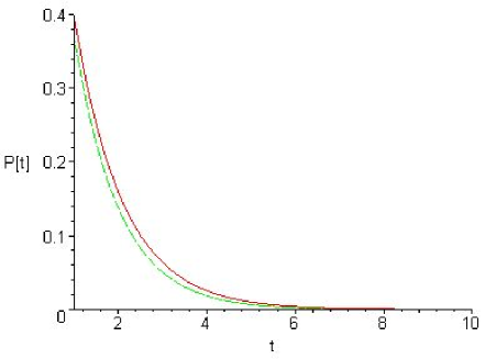
FIG. 1.: Plot on the vertical axis, commonly named $P[t]$, of the $\lambda$-corrected probability (68) (dashed line) and the harmonic probability Eq.(42) (solid line), for $\bar{\omega}=4.0\times 10^{14}/s$ and $g=\alpha\bar{\omega}$. $\alpha$ is the fine structure constant, $\alpha=1/137$ and time in units of $10^{-13}s$

VI Conclusions

In this paper we have analysed a linearized version of an particle-environment system and we have tried to give the more exact and rigorous treatment we could to the problem. We have adopted a general physicist’s point of view, in the sense that we have renounced to approach very closely to the real behaviour of a complicated non-linear system, as a quark-gluons coupled system, to study instead a linear model. As a counterpart, an exact solution has been possible.

We have presented a summary of mathematical results previously obtained, to describe an ohmic quantum system consisting of a particle (in the larger sense of a ”material body”, an atom or a Brownian particle for instance) coupled to an environment modeled by non-interacting oscillators. We have used a formalism (dressed coordinates and dressed states) that allows a non-perturbative approach to the time evolution of the system, in rather different situations as confinement or in free space. For finite $R$, our system could be seen as a simplified linear model to confined quarks and gluons inside a hadron. In this case all dressed coordinates are effectively dressed, in the sense that they are all collective, both the field modes and the particle can not be separated in this language [see Eq.(31)]. Of course the normal coordinates are also collective, but they correspond to stable eigenstates, no change in time exists for them. If we ascribe physical meaning to our dressed coordinates and states in the context of our model, matter and gauge quanta inside hadrons, can not be individualized as ”quarks” and ”gluons”, all we have is a kind of quark-gluon ”magma”. Since quarks and gluons are permanently confined, we could roughly think that, in the context of the model studied here, quarks and gluons should not really exist, they would be an artifact of perturbation theory.

In the limit $R\rightarrow\infty$, we get the result that the dressed coordinate associated to the particle describes the particle modified by the presence of the field in a indissoluble way, the particle is always dressed by the field. On the other side, the dressed harmonic modes of the field, are in the limit $R\rightarrow\infty$ identical to the bare field modes, in other words, the field keeps in the free space limit its own identity, while the particle is always accompanied by a cloud of field quanta [see Eqs.(43) and (44)].

The study on the behaviour of particles (for instance atoms in the harmonic approximation) confined in small cavities, shows that it is completelly different from the behaviour in free space. We have implicitly assumed in this study that a small cavity is still much larger than atomic dimensions (which is indeed the case for the experimental situation compared to our results, corresponding to a cavity diameter of $\sim 1\mu$), in such a way that the dressed particle could be a good approximation to the atom inside the cavity. In the first case the time evolution is very sensitive to the presence of boundaries, a fact that has been pointed out since a long time ago in the literature ([36], [37], [38]). Our dressed states approach gives an unified description for the dressing of a charged particle by the field modes and the time evolution in a cavity of arbitrary size, which includes microcavities and very large cavities (free space). If we assume that our dressed particle is a good representation for an atom under certain circumstances, we recover here with our formalism the experimental observation that excited states of atoms in sufficiently small cavities are stable for weak coupling. In the weak coupling regime, we are able to give formulas for the probability of an atom to remain excited for an infinitely long time, provided it is placed in a cavity of appropriate size. For an interaction of electromagnetic type, for an emission frequency in the visible red, the size of such cavity is in good agreement with experimental observations. Also, our approach gives an exact result for emission in free space, generalizing the well known exponential decay law. The behaviour of the system for strong coupling is rather different from its behaviour in the weak coupling regime. For appropriate cavity dimensions, which are of the same order of those ensuring stability in the weak coupling regime, we ensure for strong coupling the complete decay of the particle to the ground state in a small ellapsed time. One possible conclusion is that by changing conveniently the physical and geometric parameters (the emission frequency, the strength of the coupling and the size of the confining cavity) our formalism theoretically allows a control on the rate of emission and of the energy storage capacity (perhaps information?) in the cavity. Depending on the strength of the coupling, the emission probability ranges from a complete stability to a very rapid decay.

The formalism that we presented is rather general an applies to all systems that can be modeled by a Hamiltonian of the type given by Eq. (4). Applications to the termalization and decoherence problems will be reported elsewhere [40, 41].

VII Acknowledgements

This work received financial support from CNPq (Brazilian National Research Council).

REFERENCES

- [1] J. Glimm and A. Jaffe, Quantum Physics, a Functional Integral Point of View, Springer-Verlag - Berlin, 2nd. Ed. 1987.
- [2] C. de Calan, P.A. Faria da Veiga and J. Magnen, R. Séneor, Phys. Rev. Lett. 66, 3233 (1991).
- [3] C. Cohen-Tannoudji, Atoms in Electromagnetic Fields, World Scientific publishing Co. (1994).
- [4] A. McLachlan, Proc. Royal Soc. London, Ser. A271, 381 (1963).
- [5] J. M. Wylie and J.E. Sipe, Phys. Rev. A30, 1185 (1984).
- [6] W. Jhe and K. Jang, Phys. Rev. A53, 1126 (1996).
- [7] J. M. C. Malbouisson and B. Baseia, J. Mod. Opt. 46, 2015 (1999).
- [8] W. G. Unruh and W.H. Zurek, Phys. Rev. D40, 1071 (1989).
- [9] B. L. Hu and J. P. Paz, Yuhong Zhang, Phys, Rev. D45, 2843 (1992).
- [10] L. Davidovitch, M. Brune, J. M. Raimond and S. Haroche, Phys. Rev. A53, 1295 (1996).
- [11] K. M. Fonseca-Romero, M. C. Nemes, J. G. Peixoto de Faria, A. N. Salgueiro and A. F. R. de Toledo Piza, Phys. Rev. A58, 3205 (1998).
- [12] J.C. Le Guillou and J. Zinn-Justin, Phys. Rev. B21, 3976 (1980).
- [13] E. J. Weniger, Phys. Rev. Lett. 77, 2859 (1996).
- [14] U. D. Jentschura, Phys. Rev. A64, 013403 (2001).
- [15] G. Cvetic, C. Dib, T. Lee and I. Schmidt, hep-ph/0106024, Phys. Rev. D64 093016 (2001).
- [16] A. Ferraz de Camargo Fo., A. P. C. Malbouisson and F. R. A. Simao, J. Math. Phys. 30, 1226 (1989).
- [17] A. P. C. Malbouisson, M. A. R. Monteiro and F. R. A. Simao, J. Math. Phys. 30, 2016 (1989).
- [18] A. Ferraz de Camargo Fo., A. P. C. Malbouisson and F. R. A. Simao, J. Math. Phys. 31, 1144 (1990).
- [19] A.P.C. Malbouisson, J. Math. Phys., 35, 479 (1994).
- [20] V. Rivasseau, From Perturbative to Constructive Renormalization pp. 54-56, Princeton Univ. Press (1991).
- [21] N. Polonsky, Doctoral thesis, Ecole Normale Supérieure, Paris (1964).
- [22] S. Haroche, Doctoral thesis, Ecole Normale Supérieure, Paris (1964). ullersma,haake,caldeira,shram
- [23] N. P. Andion, A. P. C. Malbouisson and A. Mattos Neto, J.Phys. A34, 3735 (2001).
- [24] G. Flores-Hidalgo, A. P. C. Malbouisson and Y. W. Milla, Phys. Rev. A65, 063414 (2002).
- [25] P. Ullersma, Physica 32, 56, (1966); Physica 32, 74 (1966); Physica 32, 90 (1966).
- [26] F. Haake and R. Reibold, Phys. Rev. A32, 2462 (1982).
- [27] A. O. Caldeira and A. J. Legget, Ann. Phys. (N.Y) 149, 374 (1983).
- [28] H. Grabert, P. Schramm and G.-L. Ingold, Phys. Rep. 168. 115 (1988).
- [29] Notice that in any case we will consider a cavity diameter much larger than atomic dimensions. For instance, a cavity diameter of considered for an emission frequency of is of the order of times the Bohr diameter.
- [30] R.G. Hulet, E.S. Hilfer and D. Kleppner, Phys. Rev. Lett. 55, 2137 (1985).
- [31] W. Jhe, A. Anderson, E.A. Hinds, D. Meschede, L. Moi, and S. Haroche, Phys. Rev. Lett. 58, 666 (1987).
- [32] W. Thirring and F. Schwalb, Ergeb. Exakt. Naturw. 36, 219 (1964).
- [33] U. Weiss, Quantum dissipative systems, World Scientific Publishing Co., Singapore (1993).
- [34] H. Ederlyi et al.; Higher Transcendental Functions, New York, Mc Graw-Hill (1953), p. 196, formula (40).
- [35] G. Flores-Hidalgo and A. P. C. Malbouisson, Phys. Rev. A66, 042118 (2002).
- [36] H. Morawitz, Phys. Rev. A, 7, 1148 (1973).
- [37] P. Milonni and P. Knight, Opt. Comm. 9, 119 (1973).
- [38] D. Kleppner, Phys. Rev. Lett. 47, 233 (1981).
- [39] G. Flores-Hidalgo and A. P. C. Malbouisson, Phys. Lett. A311, 82 (2003).
- [40] G. Flores-Hidalgo and A. P. C. Malbouisson, The oscillator electromagnetic radiation process revisited, in preparation.
- [41] G. Flores-Hidalgo and A. P. C. Malbouisson, A non perturbative approach to the termalization process, to be submitted.