1 Introduction

It has been long acknowledged that a physically acceptable Hamiltonian is bounded below, otherwise many fundamental concepts in physics would be challenged, including the statistical interpretation of wave function and the existence of ground state. A Hamiltonian which is unbounded below would lead to negative probability and unending transition from high excited state to lower and lower energies without bound, thus making the system unstable. The criterion that a Hamiltonian should be bounded below determines which candidate Lagrangians can survive, on the most fundamental level.

An important theorem relevant to the criterion above is that a Lagrangian depends only upon the zeroth and first time derivatives, which is obtained by the 19^th century physicist Ostrogradski [1]. Allowing higher time derivatives always leads to a Hamiltonian which is not bounded below and the instability of the system. When nonlocality is introduced into Lagrangians, many new motion solutions and features emerge, some of which appear miraculous from the context of a local theory. A meaningful consequence is obtained in Ref. [2] that a Lagrangian with nonlocality of finite extent, which can be represented as the limits of higher derivatives, inherit the full Ostrogradskian instability. However, three Lagrangians of maximal nonlocality are raised in Ref. [3] to indicate that the Hamiltonian of a maximally nonlocal Lagrangian can be bounded below, so there is no generic instability of the Ostrogradskian type. In order to gain a deeper understanding of maximally nonlocal Lagrangians and apply them to quantum theory, a canonical formalism seems a necessary intermediate step towards quantization.

The purpose of this paper is to construct a canonical formalism for maximally nonlocal Lagrangians and the corresponding canonical equations. The paper is organized as follows: Section 2 is devoted to the construction of the new canonical formalism and canonical equations. This formalism is applied in Sec. 3 to the three examples raised in Ref. [3] to indicate that a maximally nonlocal Lagrangian can survive due to a bounded below Hamiltonian and to specify some important and fundamental concepts which are not emphasized in Ref. [3]. Another example is also raised in Sec. 3 to furnish a deeper understanding of the criterion concerning the stability of the system. The conclusions comprise Sec. 4.

2 Construction of Canonical Formalism and Canonical Equations

A maximally nonlocal Lagrangian is defined as one which potentially depends upon the dynamical variables from time $-T$ to time $T$, where $T$ is a large positive number approaching $+\infty$. The new Lagrangian is written in an explicit form as:

$$L=L\left({q,\dot{q},t,F(q,\dot{q})}\right)\ ,$$ (1)

where $F(q,\dot{q})$ has a general form as:

$$F(q,\dot{q})=\mathop{\lim}\limits_{T\to\infty}\int\limits_{-T}^{T}{f(q,\dot{q},t)dt}\ .$$ (2)

When dealing with such a Lagrangian, we have to make some modifications to Hamilton’s principle. In standard local cases, the arbitrary integration bounds usually cause no trouble as far as the Euler-Lagrangian equations are concerned. However, the integration bounds play such an important role in nonlocal action that different motion equations can be derived from different forms of the integration bounds [4]. Hence, we assume the integration bounds in Hamilton’s principle to be in similar forms as those in Eq. (2), i.e.

$$S=\mathop{\lim}\limits_{T\to\infty}\int\limits_{-T}^{T}{L\left({q,\dot{q},t,F(q,\dot{q})}\right)dt}\ .$$ (3)

Moreover, we make an agreement that the integration bound $T$ in Eq. (2) and Eq. (3) be considered as a constant and only when the equations of motion are obtained will $T$ approach $+\infty$. The purpose of such a procedure is to avoid some possible divergent problems [3].

According to the standard procedure, the variation of the action integral $S$ in Eq. (3) is:

$$\delta S=\mathop{\lim}\limits_{T\to\infty}\int\limits_{-T}^{T}{\left[{\frac{\partial L}{\partial q}\delta q+\frac{\partial L}{\partial\dot{q}}\delta\dot{q}+\frac{\partial L}{\partial F}\int\limits_{-T}^{T}{\left({\frac{\partial f}{\partial q}\delta q+\frac{\partial f}{\partial\dot{q}}\delta\dot{q}}\right)dt}}\right]}dt$$

$$=\mathop{\lim}\limits_{T\to\infty}\int\limits_{-T}^{T}{\left[{\frac{\partial L}{\partial q}\delta q+\frac{\partial L}{\partial\dot{q}}\delta\dot{q}+\left({\int\limits_{-T}^{T}{\frac{\partial L}{\partial F}dt}}\right)\left({\frac{\partial f}{\partial q}\delta q+\frac{\partial f}{\partial\dot{q}}\delta\dot{q}}\right)}\right]}dt\ .$$ (4)

Considering the boundary conditions

$$\mathop{\lim}\limits_{T\to\infty}\delta q(T)=\mathop{\lim}\limits_{T\to\infty}\delta q(-T)=0\ ,$$

we can obtain

$$\delta S=\mathop{\lim}\limits_{T\to\infty}\int\limits_{-T}^{T}{\left[{\frac{\partial L}{\partial q}-\frac{d}{dt}\left({\frac{\partial L}{\partial\dot{q}}}\right)+\left({\int\limits_{-T}^{T}{\frac{\partial L}{\partial F}dt}}\right)\left({\frac{\partial f}{\partial q}-\frac{d}{dt}\left({\frac{\partial f}{\partial\dot{q}}}\right)}\right)}\right]}\delta qdt\ .$$

The new equation of motion is derived from:

$$\delta S=0,\forall\delta q\ .$$ (5)

Hence, it leads to:

$$\frac{\partial L}{\partial q}-\frac{d}{dt}\left({\frac{\partial L}{\partial\dot{q}}}\right)+\left({\mathop{\lim}\limits_{T\to\infty}\int\limits_{-T}^{T}{\frac{\partial L}{\partial F}dt}}\right)\left({\frac{\partial f}{\partial q}-\frac{d}{dt}\left({\frac{\partial f}{\partial\dot{q}}}\right)}\right)=0\ .$$ (6)

We define a new function $L_{c}$ as:

$$L_{c}=L+\left({\mathop{\lim}\limits_{T\to\infty}\int\limits_{-T}^{T}{\frac{\partial L}{\partial F}dt}}\right)\cdot f\ .$$ (7)

Note that $\left({\mathop{\lim}\limits_{T\to\infty}\int\limits_{-T}^{T}{\frac{\partial L}{\partial F}dt}}\right)$ behaves like a constant as far as $\frac{\partial}{\partial q}$ and $\frac{\partial}{\partial\dot{q}}$ are concerned. The new equation of motion can be reduced to a simple form, which is similar to the local case:

$$\frac{\partial L_{c}}{\partial q}-\frac{d}{dt}\left({\frac{\partial L_{c}}{\partial\dot{q}}}\right)=0\ .$$ (8)

Before the canonical formalism is constructed, two important conserved quantities are discussed regarding the motion of maximal nonlocality. The first conserved quantity results from the homogeneity of time [5]. By virtue of this homogeneity, the properties of a system are unchanged by any displacement in time. Consider an infinitesimal displacement $\varepsilon$ in time and the corresponding change in $L$, the generalized coordinates and velocities remaining fixed, is:

$$\delta L=\frac{\partial L}{\partial t}\delta t+\frac{\partial L}{\partial F}\mathop{\lim}\limits_{T\to\infty}\int\limits_{-T}^{T}{\frac{\partial f}{\partial t}}\delta tdt$$

$$\quad=\varepsilon\cdot\left({\frac{\partial L}{\partial t}+\frac{\partial L}{\partial F}\mathop{\lim}\limits_{T\to\infty}\int\limits_{-T}^{T}{\frac{\partial f}{\partial t}}dt}\right)\ .$$ (9)

Since $\varepsilon$ is arbitrary, the condition $\delta L=0$ is equivalent to:

$$\frac{\partial L}{\partial t}+\frac{\partial L}{\partial F}\mathop{\lim}\limits_{T\to\infty}\int\limits_{-T}^{T}{\frac{\partial f}{\partial t}}dt=0\ .$$ (10)

However, as far as the motion of the maximal nonlocality is concerned, we discuss a stronger condition to satisfy the homogeneity of time, i.e.

$$\frac{\partial L}{\partial t}=0\,\,\,\mathrm{and}\,\,\,\frac{\partial f}{\partial t}=0\ .$$ (11)

Under the condition Eq. (11) and noting the definition of $L_{c}$ in Eq. (7), we can obtain:

$$\frac{\partial L_{c}}{\partial t}=0\ .$$ (12)

The total time derivative of the new function $L_{c}$ can therefore be written as,

$$\frac{dL_{c}}{dt}=\frac{\partial L_{c}}{\partial q}\dot{q}+\frac{\partial L_{c}}{\partial\dot{q}}\ddot{q}\ .$$ (13)

Replacing $\frac{\partial L_{c}}{\partial q}$, in accordance with the new equation of motion, by $\frac{d}{dt}\left({\frac{\partial L_{c}}{\partial\dot{q}}}\right)$, we obtain:

$$\frac{dL_{c}}{dt}=\dot{q}\frac{d}{dt}\left({\frac{\partial L_{c}}{\partial\dot{q}}}\right)+\frac{\partial L_{c}}{\partial\dot{q}}\ddot{q}=\frac{d}{dt}\left({\dot{q}\frac{\partial L_{c}}{\partial\dot{q}}}\right)\ ,$$ (14)

or

$$\frac{d}{dt}\left({\dot{q}\frac{\partial L_{c}}{\partial\dot{q}}-L_{c}}\right)=0\ .$$ (15)

We therefore define the energy of the system as:

$$E=\dot{q}\frac{\partial L_{c}}{\partial\dot{q}}-L_{c}\ ,$$ (16)

which, under the condition Eq. (11), is a conserved quantity during the motion of the maximal nonlocality.

The second conserved quantity follows from the homogeneity of space [5]. By virtue of this homogeneity, the properties of a system are unchanged by any parallel displacement in space. Consider an infinitesimal displacement $\varepsilon$ in space and the corresponding change in $L$, the generalized velocities remaining fixed, is:

$$\delta L=\frac{\partial L}{\partial q}\delta q+\frac{\partial L}{\partial F}\mathop{\lim}\limits_{T\to\infty}\int\limits_{-T}^{T}{\frac{\partial f}{\partial q}}\delta qdt$$

$$\quad=\varepsilon\cdot\left({\frac{\partial L}{\partial q}+\frac{\partial L}{\partial F}\mathop{\lim}\limits_{T\to\infty}\int\limits_{-T}^{T}{\frac{\partial f}{\partial q}}dt}\right)\ .$$ (17)

Since $\varepsilon$ is arbitrary, the condition $\delta L=0$ is equivalent to:

$$\frac{\partial L}{\partial q}+\frac{\partial L}{\partial F}\mathop{\lim}\limits_{T\to\infty}\int\limits_{-T}^{T}{\frac{\partial f}{\partial q}}dt=0\ .$$ (18)

Similarly, as far as the motion of the maximal nonlocality is concerned, we discuss a stronger condition to satisfy the homogeneity of space, i.e.

$$\frac{\partial L}{\partial q}=0\,\,\,\mathrm{and}\,\,\,\frac{\partial f}{\partial q}=0\ .$$ (19)

Under the condition Eq. (19) and noting the definition of $L_{c}$ in Eq. (7), we can obtain:

$$\frac{\partial L_{c}}{\partial q}=0\ .$$ (20)

By the new equation of motion Eq. (8), Eq. (20) is equivalent to:

$$\frac{d}{dt}\left({\frac{\partial L_{c}}{\partial\dot{q}}}\right)=0\ .$$ (21)

We define the canonical momentum of the system as:

$$p^{\ast}=\frac{\partial L_{c}}{\partial\dot{q}}\ ,$$ (22)

which, under the condition Eq. (19), is a conserved quantity during the motion of the maximal nonlocality.

By the Legendre transformation, we change the variables from $(q,\dot{q},t)$ to $(q,p^{\ast},t)$ and define the new Hamiltonian as:

$$H^{\ast}\left({q,p^{\ast},t,G(q,p^{\ast})}\right)\equiv p^{\ast}q-L_{c}\left({q,\dot{q},t,F(q,\dot{q})}\right)\ .$$ (23)

Note that as the Hamiltonian depends on $q,p^{\ast}$and $t$ only, the generalized velocity $\dot{q}$ has to be converted into the function of $q,p^{\ast},t$ and $G(q,p^{\ast})$, where $G(q,p^{\ast})$ has a general form as:

$$G(q,p^{\ast})=\mathop{\lim}\limits_{T\to\infty}\int\limits_{-T}^{T}{g(q,p^{\ast},t)dt}\ .$$ (24)

A general method of converting $\dot{q}$ to $\dot{q}=\dot{q}\left({q,p^{\ast},t,G(q,p^{\ast})}\right)$ is furnished below.

By the definition of $p^{\ast}$ in Eq. (22), we can obtain a general expression of the new canonical momentum:

$$p^{\ast}=p^{\ast}\left({q,\dot{q},t,F(q,\dot{q})}\right)\ ,$$ (25)

where $F(q,\dot{q})$ has a general form as $\mathop{\lim}\limits_{T\to\infty}\int\limits_{-T}^{T}{f(q,\dot{q},t)dt}$. Let $F(q,\dot{q})$ be $\gamma$ and assume that $\dot{q}$ can be solved from Eq. (25), i.e.

$$\dot{q}=\dot{q}\left({q,p^{\ast},t,\gamma}\right)\ ,$$ (26)

then substitute Eq. (26) into the general form of $F(q,\dot{q})$ and we obtain:

$$\mathop{\lim}\limits_{T\to\infty}\int\limits_{-T}^{T}{f\left({q,\dot{q}(q,p^{\ast},t,\gamma),t}\right)dt=\gamma}\ .$$ (27)

This is the algebra equation for $\gamma$. The solution of Eq. (27) is denoted as $\gamma_{0}$, which is the function of $G(q,p^{\ast})$, where $G(q,p^{\ast})$ has a general form as $\mathop{\lim}\limits_{T\to\infty}\int\limits_{-T}^{T}{g(q,p^{\ast},t)dt}$. Substitute the solution $\gamma_{0}\left({G(q,p^{\ast})}\right)$ back into Eq. (26) we obtain:

$$\dot{q}=\dot{q}\left({q,p^{\ast},t,\gamma_{{}_{0}}\left({G(q,p^{\ast},t)}\right)}\right)\ .$$ (28)

Considered as a function of $q,p^{\ast}$ and $t$ only, the differential of $H^{\ast}$is given by:

$$dH^{\ast}=\frac{\partial H^{\ast}}{\partial q}dq+\frac{\partial H^{\ast}}{\partial p^{\ast}}dp^{\ast}+\frac{\partial H^{\ast}}{\partial t}dt\ .$$ (29)

It is emphasized again that as far as $\frac{\partial}{\partial q}$ and $\frac{\partial}{\partial p^{\ast}}$ are concerned, $G(q,p^{\ast})=\mathop{\lim}\limits_{T\to\infty}\int\limits_{-T}^{T}{g(q,p^{\ast},t)dt}$ is considered as a constant. But from the defining equation (23), we can also write:

$$dH^{\ast}=d\left({p^{\ast}\dot{q}-L_{c}}\right)=\dot{p}^{\ast}dq+\dot{q}dp^{\ast}-dL_{c}\ .$$ (30)

Considered as a function of $q,\dot{q}$ and $t$ only, the differential of $L_{c}$is given by:

$$dL_{c}=\frac{\partial L_{c}}{\partial q}dq+\frac{\partial L_{c}}{\partial\dot{q}}d\dot{q}+\frac{\partial L_{c}}{\partial t}dt\ .$$ (31)

Noting the definition of $p^{\ast}$ (22) and the equation of motion Eq. (8), we can reduce Eq. (31) to a simple form:

$$dL_{c}=\dot{p}^{\ast}dq+p^{\ast}d\dot{q}+\frac{\partial L_{c}}{\partial t}dt\ .$$ (32)

Substituting Eq. (32) into Eq. (30), we can obtain:

$$dH^{\ast}=-\dot{p}^{\ast}dq+\dot{q}dp^{\ast}-\frac{\partial L_{c}}{\partial t}dt\ .$$ (33)

Comparison of Eq. (33) with Eq. (29) leads to the new canonical equations of Hamiltonian:

$$\left\{{\begin{array}[]{l}\frac{\partial H^{\ast}}{\partial p^{\ast}}=\dot{q}\ ,\\ \frac{\partial H^{\ast}}{\partial q}=-\dot{p}^{\ast}\ ,\\ \frac{\partial H^{\ast}}{\partial t}=-\frac{\partial L_{c}}{\partial t}\ ,\\ \end{array}}\right.$$ (34)

which are similar to those of local cases.

3 A FEW EXAMPLES

Applications of the new canonical formalism and canonical equations are illustrated in this section, where $\mathop{\lim}\limits_{T\to\infty}$ will be omitted for the sake of conciseness and convenience. The implication of the integration bound accords with the agreement in Sec. 2. The new canonical formalism and canonical equations are first applied to the three Lagrangians in Ref. [3].

Consider the first Lagrangian:

$$L=\frac{1}{2}m\dot{q}^{2}-\frac{1}{4}m\omega_{0}^{2}q^{2}\int\limits_{-T}^{T}{\frac{q^{2}}{l_{0}^{2}}}\frac{dt}{T}\ ,$$ (35)

where $F(q,\dot{q})=\int\limits_{-T}^{T}{\frac{q^{2}}{l_{0}^{2}}}\frac{dt}{T}$ and $f(q,\dot{q},t)=\frac{q^{2}}{Tl_{0}^{2}}\ .$ The new function $L_{c}$ can be derived from Eq. (7):

$$L_{c}=L+\left({\int\limits_{-T}^{T}{\frac{\partial L}{\partial F}dt}}\right)\cdot f=\frac{1}{2}m\dot{q}^{2}-\frac{1}{2}m\omega_{0}^{2}q^{2}\int\limits_{-T}^{T}{\frac{q^{2}}{l_{0}^{2}}\frac{dt}{T}}\ .$$ (36)

The energy of the system is:

$$E=\dot{q}\frac{\partial L_{c}}{\partial\dot{q}}-L_{c}=\frac{1}{2}m\dot{q}^{2}+\frac{1}{2}m\omega_{0}^{2}q^{2}\int\limits_{-T}^{T}{\frac{q^{2}}{l_{0}^{2}}\frac{dt}{T}}\ ,$$ (37)

which is conserved as the condition Eq. (12) is satisfied. The canonical momentum is:

$$p^{\ast}=\frac{\partial L_{c}}{\partial\dot{q}}=m\dot{q}\ .$$ (38)

Convert $\dot{q}$ to:

$$\dot{q}=\frac{p^{\ast}}{m}\ ,$$ (39)

we can obtain the new Hamiltonian from Eq. (36) and Eq. (39):

$$H^{\ast}=p^{\ast}\dot{q}-L_{c}=\frac{(p^{\ast})^{2}}{2m}+\frac{1}{2}m\omega_{0}^{2}q^{2}\int\limits_{-T}^{T}{\frac{q^{2}}{l_{0}^{2}}\frac{dt}{T}}\ .$$ (40)

By the new canonical equation (34), the equation of motion reads:

$$\ddot{q}+\omega^{2}q=0\ ,$$ (41)

where

$$\omega^{2}=\omega_{0}^{2}\int\limits_{-T}^{T}{\frac{q^{2}}{l_{0}^{2}}}\frac{dt}{T}\ .$$ (42)

It is in accordance with Eq. (10-11) in Ref. [3].

Consider the second Lagrangian:

$$L=\frac{1}{2}m\dot{q}^{2}-\frac{1}{4}m\omega_{0}^{2}q^{2}-\frac{1}{16}m\omega_{0}^{2}l_{0}^{2}\sin\left({\frac{2}{T}\int\limits_{-T}^{T}{\frac{q^{2}}{l_{0}^{2}}}dt}\right)\ .$$ (43)

where $F(q,\dot{q})=2\int\limits_{-T}^{T}{\frac{q^{2}}{l_{0}^{2}}}\frac{dt}{T}$ and $f(q,\dot{q},t)=\frac{2q^{2}}{Tl_{0}^{2}}$. Repeating the same procedure, we have:

$$L_{c}=\frac{1}{2}m\dot{q}^{2}-\frac{1}{2}m\omega_{0}^{2}q^{2}\cos^{2}\left({2\int\limits_{-T}^{T}{\frac{q^{2}}{l_{0}^{2}}}\frac{dt}{T}}\right)-\frac{1}{16}m\omega_{0}^{2}l_{0}^{2}\sin\left({2\int\limits_{-T}^{T}{\frac{q^{2}}{l_{0}^{2}}}\frac{dt}{T}}\right)\ .$$ (44)

The energy of the system, which is conserved as the condition Eq. (11) is satisfied, is:

$$E=\frac{1}{2}m\dot{q}^{2}+\frac{1}{2}m\omega_{0}^{2}q^{2}\cos^{2}\left({2\int\limits_{-T}^{T}{\frac{q^{2}}{l_{0}^{2}}}\frac{dt}{T}}\right)+\frac{1}{16}m\omega_{0}^{2}l_{0}^{2}\sin\left({2\int\limits_{-T}^{T}{\frac{q^{2}}{l_{0}^{2}}}\frac{dt}{T}}\right)\ ,$$ (45)

which accords with the energy defined in Ref. [3] except for the last added term on the $r.$$h.$$s.$ of the above equation. The canonical momentum is:

$$p^{\ast}=\frac{\partial L_{c}}{\partial\dot{q}}=m\dot{q}\ ,$$ (46)

or

$$\dot{q}=\frac{p^{\ast}}{m}\ .$$ (47)

The Hamiltonian is:

$$H^{\ast}=\frac{(p^{\ast})^{2}}{2m}+\frac{1}{2}m\omega_{0}^{2}q^{2}\cos^{2}\left({2\int\limits_{-T}^{T}{\frac{q^{2}}{l_{0}^{2}}}\frac{dt}{T}}\right)+\frac{1}{16}m\omega_{0}^{2}l_{0}^{2}\sin\left({2\int\limits_{-T}^{T}{\frac{q^{2}}{l_{0}^{2}}}\frac{dt}{T}}\right)\ ,$$ (48)

and the equation of motion follows:

$$\ddot{q}+\omega^{2}q=0\ ,$$ (49)

where

$$\omega^{2}=\omega_{0}^{2}\cos^{2}\left({\int\limits_{-T}^{T}{\frac{q^{2}}{l_{0}^{2}}}\frac{dt}{T}}\right)\ .$$ (50)

It is in accordance with Eq. (20-21) in Ref. [3].

Now consider the third Lagrangian whose consequences will be a little different from those in Ref. [3].

$$L=-\frac{1}{4}m\omega_{0}^{2}l_{0}^{2}\exp\left({-\int\limits_{-T}^{T}{\frac{\dot{q}^{2}}{\omega_{0}^{2}l_{0}^{2}}\frac{dt}{T}}}\right)-\frac{1}{2}m\omega_{0}^{2}q^{2}\ ,$$ (51)

where $F(q,\dot{q})=-\int\limits_{-T}^{T}{\frac{\dot{q}^{2}}{\omega_{0}^{2}l_{0}^{2}}\frac{dt}{T}}$ and $f(q,\dot{q},t)=\frac{\dot{q}^{2}}{\omega_{0}^{2}l_{0}^{2}T}$. The new function $L_{c}$ can be derived from Eq. (7):

$$L_{c}=\frac{1}{2}m\dot{q}^{2}\exp\left({-\int\limits_{-T}^{T}{\frac{\dot{q}^{2}}{\omega_{0}^{2}l_{0}^{2}}\frac{dt}{T}}}\right)-\frac{1}{2}m\omega_{0}^{2}q^{2}-\frac{1}{4}m\omega_{0}^{2}l_{0}^{2}\exp\left({-\int\limits_{-T}^{T}{\frac{\dot{q}^{2}}{\omega_{0}^{2}l_{0}^{2}}\frac{dt}{T}}}\right)\ .$$ (52)

The energy of the system, which can be derived from Eq. (16), follows:

$$E=\frac{1}{2}m\dot{q}^{2}\exp\left({-\int\limits_{-T}^{T}{\frac{\dot{q}^{2}}{\omega_{0}^{2}l_{0}^{2}}\frac{dt}{T}}}\right)+\frac{1}{2}m\omega_{0}^{2}q^{2}+\frac{1}{4}m\omega_{0}^{2}l_{0}^{2}\exp\left({-\int\limits_{-T}^{T}{\frac{\dot{q}^{2}}{\omega_{0}^{2}l_{0}^{2}}\frac{dt}{T}}}\right)\ ,$$ (53)

which is conserved as the condition Eq. (11) is satisfied. The canonical momentum is:

$$p^{\ast}=m\dot{q}\exp\left({-\int\limits_{-T}^{T}{\frac{\dot{q}^{2}}{\omega_{0}^{2}l_{0}^{2}}\frac{dt}{T}}}\right)\ .$$ (54)

According to the general method in Sec. 2, let $-\int\limits_{-T}^{T}{\frac{\dot{q}^{2}}{\omega_{0}^{2}l_{0}^{2}}\frac{dt}{T}}$ be $\gamma$:

$$p^{\ast}=m\dot{q}e^{\gamma}$$ (55)

or

$$\dot{q}=\frac{p^{\ast}}{m}e^{-\gamma}\ .$$ (56)

Substitute Eq. (56) into the explicit expression of $\gamma$ we obtain:

$$-\int\limits_{-T}^{T}{\frac{1}{\omega_{0}^{2}l_{0}^{2}}\frac{(p^{\ast})^{2}}{m^{2}}e^{-2\gamma}\frac{dt}{T}}=\gamma\ .$$ (57)

Now let $-\int\limits_{-T}^{T}{\frac{1}{\omega_{0}^{2}l_{0}^{2}}\frac{(p^{\ast})^{2}}{m^{2}}\frac{dt}{T}}$ be $\alpha$ and Eq. (57) is recast as:

$$\gamma e^{2\gamma}=\alpha\ .$$ (58)

The Eq. (58) is the algebra equation with respect to $\gamma$, whose solution is determined by $\alpha$. Assume that the solution to Eq. (58) is:

$$\gamma_{0}=\gamma_{0}(\alpha)\ ,$$ (59)

and substitute the solution Eq. (59) back into Eq. (56) we get:

$$\dot{q}=\frac{p^{\ast}}{m}e^{-\gamma_{0}(\alpha)}\ ,$$ (60)

where $\alpha=-\int\limits_{-T}^{T}{\frac{1}{\omega_{0}^{2}l_{0}^{2}}\frac{(p^{\ast})^{2}}{m^{2}}\frac{dt}{T}}$. The new Hamiltonian follows, noting that $\dot{q}$ has to appear in the form of Eq. (60) in the Hamiltonian:

$$H^{\ast}=\frac{(p^{\ast})^{2}}{2m}e^{-\gamma_{0}(\alpha)}+\frac{1}{2}m\omega_{0}^{2}q^{2}+\frac{1}{4}m\omega_{0}^{2}l_{0}^{2}e^{\gamma_{0}(\alpha)}\ .$$ (61)

The equation of motion follows:

$$\ddot{q}+\omega^{2}q=0\ ,$$ (62)

where

$$\omega^{2}=\omega_{0}^{2}\exp\left({\int\limits_{-T}^{T}{\frac{\dot{q}^{2}}{\omega_{0}^{2}l_{0}^{2}}\frac{dt}{T}}}\right)\ .$$ (63)

According to the method in Ref. [3], the general solution to Eq. (62) is:

$$q(t)=q_{0}\cos\omega t+\frac{\dot{q}_{0}}{\omega}\sin\omega t\ .$$ (64)

Substituting Eq. (64) into Eq. (63), we can obtain an algebra equation with respect to $\omega$ (Note that $T$ approaches $+\infty$.):

$$\omega^{2}=\omega_{0}^{2}\exp\left({\frac{\omega^{2}q_{0}^{2}+\dot{q}_{0}^{2}}{\omega_{0}^{2}l_{0}^{2}}}\right)\ .$$ (65)

One thing we should pay attention to is that from the solution Eq. (64), it is taken for granted in Ref. [3] that the energy of the system is:

$$E=\frac{1}{2}m\dot{q}^{2}+\frac{1}{2}m\omega^{2}q^{2}\ ,$$ (66)

where $\omega$ is determined by Eq. (65). However, substituting the general solution Eq. (64) into $\exp\left({-\int\limits_{-T}^{T}{\frac{\dot{q}^{2}}{\omega_{0}^{2}l_{0}^{2}}\frac{dt}{T}}}\right)$ in Eq. (53) and we can obtain:

$$E=\frac{1}{2}m\dot{q}^{2}\exp\left({-\frac{\omega^{2}q_{0}^{2}+\dot{q}_{0}^{2}}{\omega_{0}^{2}l_{0}^{2}}}\right)+\frac{1}{2}m\omega_{0}^{2}q^{2}+\frac{1}{4}m\omega_{0}^{2}l_{0}^{2}\exp\left({-\frac{\omega^{2}q_{0}^{2}+\dot{q}_{0}^{2}}{\omega_{0}^{2}l_{0}^{2}}}\right)\ .$$ (67)

Note Eq. (65) and reduce Eq. (67) to:

$$E=\frac{1}{2}m\dot{q}^{2}\left({\frac{\omega_{0}^{2}}{\omega^{2}}}\right)+\frac{1}{2}m\omega_{0}^{2}q^{2}+\frac{1}{4}m\omega_{0}^{2}l_{0}^{2}\left({\frac{\omega_{0}^{2}}{\omega^{2}}}\right)$$

$$=\left({\frac{\omega_{0}^{2}}{\omega^{2}}}\right)\left({\frac{1}{2}m\dot{q}^{2}+\frac{1}{2}m\omega^{2}q^{2}+\frac{1}{4}m\omega_{0}^{2}l_{0}^{2}}\right)\ ,$$ (68)

where $\omega$ is also determined by Eq. (65).

The Eq. (68) indicates that for every solution $\omega^{2}$, the energy of the system is not the familiar form Eq. (66) but rather a new form Eq. (68) which, if the added constant $\frac{\omega_{0}^{2}}{\omega^{2}}\frac{1}{4}m\omega_{0}^{2}l_{0}^{2}$ is not taken into consideration, is the product of Eq. (66) with $\frac{\omega_{0}^{2}}{\omega^{2}}$. But $\omega^{2}$ is not equal to $\omega_{0}^{2}$ except for specific initial value data to satisfy Eq. (65), illustrating that Eq. (68) is not equal to Eq. (66) on most occasions. The reason why the kinetic energy is not equal to $\frac{1}{2}m\dot{q}^{2}$ is that the rule determining the equations of motion is no longer Newton’s second law, which leads to a new definition of the kinetic energy.

The kinetic energy $T$ is defined in general to be:

$$\mbox{ }dT\equiv\frac{dp^{\ast}}{dt}dq=\dot{q}dp^{\ast}\ ,$$ (69)

where $p^{\ast}$ is the new canonical momentum defined by Eq. (22). Applying Eq. (69) to the previous example, we can obtain the new kinetic energy from Eq. (54):

$$dT=\dot{q}dp^{\ast}=\dot{q}d\left({m\dot{q}\exp\left({-\int\limits_{-T}^{T}{\frac{\dot{q}^{2}}{\omega_{0}^{2}l_{0}^{2}}\frac{dt}{T}}}\right)}\right)$$

$$=d\left({\frac{1}{2}m\dot{q}^{2}\exp\left({-\int\limits_{-T}^{T}{\frac{\dot{q}^{2}}{\omega_{0}^{2}l_{0}^{2}}\frac{dt}{T}}}\right)}\right)\ .$$ (70)

Substituting the general solution Eq. (64) into Eq. (70) and noting the algebra equation Eq. (65), we can obtain that for every solution $\omega^{2}$, the new kinetic energy is:

$$dT=d\left({\frac{1}{2}m\dot{q}^{2}\frac{\omega_{0}^{2}}{\omega^{2}}}\right)\ ,$$ (71)

which accords with Eq. (68). However, the difference in Eq. (66) and Eq. (68) does not disputes the conclusion that such a harmonic oscillator is stable as for every oscillatory solution, $\omega^{2}$ is positive, which means that Eq. (68) is bounded below.

In above we discussed the three examples given in Ref. [3]. In the following we construct a new example which gives a deeper insight into the difference between the familiar form Eq. (66) and the correct definition of the system energy Eq. (16), from which we can find that the stability of system and the form of solutions to the equations of motion have a more complicated relation in maximally nonlocal action than that of local case. To understand it, consider the following maximally nonlocal harmonic oscillator:

$$L=-m\omega_{0}^{2}q^{2}\cos\left({\int\limits_{-T}^{T}{\frac{\dot{q}^{2}}{\omega_{0}^{2}l_{0}^{2}}\frac{dt}{T}}}\right)+\frac{1}{2}m\omega_{0}^{2}l_{0}^{2}G\left({\int\limits_{-T}^{T}{\frac{\dot{q}^{2}}{\omega_{0}^{2}l_{0}^{2}}\frac{dt}{T}}}\right)\ ,$$ (72)

where $G(t)$ is a shorthand for:

$$G(t)=\frac{1}{2}e^{t}\left[{\sin t-t\left({\sin t-\cos t}\right)}\right]\ .$$ (73)

The new function $L_{c}$can be derived from Eq. (7):

$$L_{c} = -m\omega_{0}^{2}q^{2}\cos\left({\int\limits_{-T}^{T}{\frac{\dot{q}^{2}}{\omega_{0}^{2}l_{0}^{2}}\frac{dt}{T}}}\right)+\frac{1}{2}m\omega_{0}^{2}l_{0}^{2}G\left({\int\limits_{-T}^{T}{\frac{\dot{q}^{2}}{\omega_{0}^{2}l_{0}^{2}}\frac{dt}{T}}}\right)$$ (74)

$$+m\dot{q}^{2}\int\limits_{-T}^{T}{\frac{q^{2}}{l_{0}^{2}}\frac{dt}{T}\sin\left({\int\limits_{-T}^{T}{\frac{\dot{q}^{2}}{\omega_{0}^{2}l_{0}^{2}}\frac{dt}{T}}}\right)}+m\dot{q}^{2}g\left({\int\limits_{-T}^{T}{\frac{\dot{q}^{2}}{\omega_{0}^{2}l_{0}^{2}}\frac{dt}{T}}}\right)\ ,$$

where $g(t)$ is a shorthand for:

$$g(t)=G^{\prime}(t)=e^{t}\left({\cos t-t\sin t}\right)\ .$$ (75)

By the equation of motion with respect to $L_{c}$ given by Eq. (8), we can obtain:

$$\ddot{q}+\omega^{2}q=0\ .$$ (76)

where

$$\omega^{2}=\omega_{0}^{2}\frac{\cos\left({\int\limits_{-T}^{T}{\frac{\dot{q}^{2}}{\omega_{0}^{2}l_{0}^{2}}\frac{dt}{T}}}\right)}{\int\limits_{-T}^{T}{\frac{q^{2}}{l_{0}^{2}}\frac{dt}{T}\sin\left({\int\limits_{-T}^{T}{\frac{\dot{q}^{2}}{\omega_{0}^{2}l_{0}^{2}}\frac{dt}{T}}}\right)}+g\left({\int\limits_{-T}^{T}{\frac{\dot{q}^{2}}{\omega_{0}^{2}l_{0}^{2}}\frac{dt}{T}}}\right)}\ .$$ (77)

The general solution to Eq. (76) has the following form:

$$q(t)=q_{0}\cos\omega t+\frac{\dot{q}_{0}}{\omega}\sin\omega t\ .$$ (78)

Consider a specific situation that the initial coordinate $q_{0}$ is zero and the initial velocity $\dot{q}_{0}$ is arbitrary:

$$q(t)=\frac{\dot{q}_{0}}{\omega}\sin\omega t\ .$$ (79)

Substitute the solution Eq. (79) into Eq. (77) we obtain:

$$\omega^{2}=\omega_{0}^{2}\frac{\cos\left({\frac{\dot{q}_{0}^{2}}{\omega_{0}^{2}l_{0}^{2}}}\right)}{\frac{\dot{q}_{0}^{2}}{\omega^{2}l_{0}^{2}}\sin\left({\frac{\dot{q}_{0}^{2}}{\omega_{0}^{2}l_{0}^{2}}}\right)+g\left({\frac{\dot{q}_{0}^{2}}{\omega_{0}^{2}l_{0}^{2}}}\right)}\ .$$ (80)

Let $\frac{\dot{q}_{0}^{2}}{\omega_{0}^{2}l_{0}^{2}}$ be $t$ and Eq. (80) is reduced to:

$$\omega^{2}=\omega_{0}^{2}\frac{\cos t}{\frac{\omega_{0}^{2}}{\omega^{2}}t\sin t+g(t)}\ .$$ (81)

This equation can be converted to a more explicit expression:

$$\omega^{2}=\omega_{0}^{2}\frac{\cos t-t\sin t}{g(t)}\ .$$ (82)

Substitute the explicit expression of $g(t)$, Eq. (75), into Eq. (82) we get:

$$\omega^{2}=\omega_{0}^{2}e^{-t}\ ,$$ (83)

from which we read off that for every initial value $(0,\dot{q})$, $\omega^{2}$ is always positive which means an oscillatory solution. The energy of the system, defined by Eq. (16), follows:

$$E = m\dot{q}^{2}\int\limits_{-T}^{T}{\frac{q^{2}}{l_{0}^{2}}\frac{dt}{T}\sin\left({\int\limits_{-T}^{T}{\frac{\dot{q}^{2}}{\omega_{0}^{2}l_{0}^{2}}\frac{dt}{T}}}\right)}+m\dot{q}^{2}g\left({\int\limits_{-T}^{T}{\frac{\dot{q}^{2}}{\omega_{0}^{2}l_{0}^{2}}\frac{dt}{T}}}\right)$$ (84)

$$+m\omega_{0}^{2}q^{2}\cos\left({\int\limits_{-T}^{T}{\frac{\dot{q}^{2}}{\omega_{0}^{2}l_{0}^{2}}\frac{dt}{T}}}\right)-\frac{1}{2}m\omega_{0}^{2}l_{0}^{2}G\left({\int\limits_{-T}^{T}{\frac{\dot{q}^{2}}{\omega_{0}^{2}l_{0}^{2}}\frac{dt}{T}}}\right)\ .$$

Noting the definition of $\omega^{2}$ Eq. (77), we reduce Eq. (84) to:

$$E = \left[{\int\limits_{-T}^{T}{\frac{q^{2}}{l_{0}^{2}}\frac{dt}{T}\sin\left({\int\limits_{-T}^{T}{\frac{\dot{q}^{2}}{\omega_{0}^{2}l_{0}^{2}}\frac{dt}{T}}}\right)}+g\left({\int\limits_{-T}^{T}{\frac{\dot{q}^{2}}{\omega_{0}^{2}l_{0}^{2}}\frac{dt}{T}}}\right)}\right]\left({m\dot{q}^{2}+m\omega^{2}q^{2}}\right)$$

$$-\frac{1}{2}m\omega_{0}^{2}l_{0}^{2}G\left({\int\limits_{-T}^{T}{\frac{\dot{q}^{2}}{\omega_{0}^{2}l_{0}^{2}}\frac{dt}{T}}}\right)$$

$$= \frac{\omega_{0}^{2}}{\omega^{2}}\cos\left({\int\limits_{-T}^{T}{\frac{\dot{q}^{2}}{\omega_{0}^{2}l_{0}^{2}}\frac{dt}{T}}}\right)\left({m\dot{q}^{2}+m\omega^{2}q^{2}}\right)-\frac{1}{2}m\omega_{0}^{2}l_{0}^{2}G\left({\int\limits_{-T}^{T}{\frac{\dot{q}^{2}}{\omega_{0}^{2}l_{0}^{2}}\frac{dt}{T}}}\right)$$

$$\ .$$ (85)

Substitute the solution Eq. (79) and Eq. (83) into Eq. (3):

$$E=m\omega_{0}^{2}l_{0}^{2}te^{t}\cos t-\frac{1}{2}m\omega_{0}^{2}l_{0}^{2}G(t)\ .$$ (86)

where $t$ is a shorthand for $\frac{\dot{q}_{0}^{2}}{\omega_{0}^{2}l_{0}^{2}}$. Note the explicit expression of $G(t)$:

$$E=\frac{1}{4}m\omega_{0}^{2}l_{0}^{2}te^{t}\left({3\cos t+\sin t-\frac{\sin t}{t}}\right)\ .$$ (87)

In fig. 1 we plot qualitatively the dependence of the energy on $t$, which illustrates that the energy of system Eq. (87) is unbounded below. Noting an important fact that the Hamiltonian and the energy of system are the same quantity in two different representations when the condition Eq. (12) is satisfied, we can infer that the maximally nonlocal harmonic oscillator Eq. (72) is unstable, which is contrary to the conclusion of a local case.

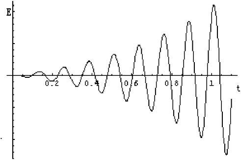
Figure 1: The qualitative behavior of the energy as a function of t.

It is argued in Ref. [6] that a harmonic oscillator with an unbounded below Hamiltonian is not surprising, since one can get a simple example by reversing the sign of the harmonic oscillator Lagrangian:

$$L=-\frac{1}{2}m\dot{q}^{2}+\frac{1}{2}m\omega_{0}^{2}q^{2}\ ,$$ (88)

which does not alter the oscillatory solution but the corresponding Hamiltonian is unbounded below:

$$H=-\frac{1}{2}m\dot{q}^{2}-\frac{1}{2}m\omega_{0}^{2}q^{2}\ .$$ (89)

However, reversing the sign of the Lagrangian, in essence, changes the definition of energy. From Eq. (16), we can easily obtain that the energy is defined as a conserved quantity during the motion when the condition Eq. (11) is satisfied. If the defined energy $E$ is conserved, $-E$ is also conserved but a stable system requires its energy $E$ (more literally, its Hamiltonian) to be bounded below, thus meaning that arbitrary definition of energy would lead to contradictory conclusions concerning the stability of system.

One thing we should pay attention to is the correspondence principle which can determine some constants that would otherwise be arbitrary in new physics. The energy of a classical harmonic oscillator is:

$$E=\frac{1}{2}m\dot{q}_{0}^{2}+\frac{1}{2}m\omega_{0}^{2}q_{0}^{2}\ ,$$ (90)

where $q_{0},\dot{q}_{0}$ are the initial values. (Eq. (88) is meaningless in classical physics.) When the energy is low, the maximally nonlocal harmonic oscillator should be degenerated to its classical form Eq. (90). Note that when $t=\frac{\dot{q}_{0}^{2}}{\omega_{0}^{2}l_{0}^{2}}$ is a small number, Eq. (87) is approximate to:

$$E\approx\frac{1}{2}m\omega_{0}^{2}l_{0}^{2}t=\frac{1}{2}m\dot{q}_{0}^{2}\ ,$$ (91)

which accords with the classical form Eq. (90). The correspondence principle justifies the definition of energy Eq. (16) and further confirms that the maximally nonlocal harmonic oscillatory Eq. (72), though its energy has a classical limit, is actually unstable when the initial values are large enough to result in deep negative energy.

4 Conclusions

We have established the canonical formalism of maximally nonlocal Lagrangian by the Legendre transformation to the new function $L_{c}$ (7). We have also shown that when the conditions Eq. (7) and Eq. (11) are satisfied, two important conserved quantities exist, both of which can be derived from the new function $L_{c}$. It is easy to conclude that the new function $L_{c}$ behaves much like the Lagrangian in local theory in that standard procedures can remain as long as the new function $L_{c}$ substitutes the original Lagrangian. And $L_{c}$ differs from the original Lagrangian only when the functional of the dynamical variables is introduced into the Lagrangian and Hamilton’s principle is modified to fit the maximally nonlocal Lagrangian.

The examples we have discussed above illustrate that with the new definition of the energy of system (more literally the canonical Hamiltonian), more complicated physical properties emerge in the maximally nonlocal action, some of which differ drastically with those of local cases. The difference culminates in the last example as the positivity of the energy of a harmonic oscillatory is demolished and the unbounded negative energy is derived from the new definition of the energy.

Acknowledgments

This work was partially supported by the “Principal Fund” of Peking University.

References

[1] M. Ostrogradski, Mem. Ac. St. Petersbourg VI 4,
385(1850).
[2] R. P. Woodard, Phys. Rev. A62, 052105(2000).
[3] D. L. Bennett, H. B. Nielsen, and R. P. Woodard, Phys. Rev.
D57, 1167(1998).
[4] J. Llosa, Phys. Rev. A67, 016101(2003).
[5] L. D. Landau and E. M. Lifshitz, Mechanics; Third
Edition, Butterworth Heinemann, 1976.