Two-fermion relativistic bound states in Light-Front Dynamics

Abstract

In the Light-Front Dynamics, the wave function equations and their numerical solutions, for two fermion bound systems, are presented. Analytical expressions for the ladder one-boson exchange interaction kernels corresponding to scalar, pseudoscalar, pseudovector and vector exchanges are given. Different couplings are analyzed separately and each of them is found to exhibit special features. The results are compared with the non relativistic solutions.

I Introduction

The two-fermion system covers a huge number of applications in atomic (e⁺e^-), nuclear (NN, N̄N) and subnuclear (qq̄) physics. The interest in using a relativistic description for such systems appeared in the early days of quantum mechanics KGE ; Dirac_PRSL_A117_28 and has constantly been pursued since by many authors. This interest has recently found a new élan due to the measurements performed at Jefferson Laboratory JLAB_ed_98 ; JLAB_AQ2_A_99 ; JLAB_AQ2_C_99 ; JLAB_t20_00 where simple nuclear systems have been – and are being – probed at momentum transfers much larger than their constituent masses. This experimental activity motivated a consequent number of works on relativistic dynamics. Extensive reviews on the past and recent deuteron results can be found in GVO ; GG .

Most of the approaches developed for describing relativistic two-body systems are based on Bethe-Salpeter (BS) equation BS_51 ; FT_PRD21_80 ; ZT_PRC22_80 ; VFT_PRC33_86 ; RT_PRC45_92 ; PA_PRC54_96 ; BBMST_02 or three-dimensional reductions of it LT_63 ; BBS_66 ; Gross ; Gross_et_al ; Wallace ; HT_PRC42_90 .

An alternative approach is provided by the Light-Front Dynamics (LFD). In its standard version, following Dirac’s classification of relativistic theories Dirac_49 , the state vector is defined on the $\sigma=z+t$ surface. Wave functions - defined as the Fock components of the state vector - are the formal objects of this theory and are directly comparable to their non relativistic counterparts. LFD has been developed and used by many authors LS_AP_78 ; CCKP_PRC37_88 ; COESTER_92 ; Fuda_90 ; FZ_PRC_95 ; Ji_94 ; Burkart_96 ; BKT_NPB158_79 ; LB_PRD52_95_2 ; SB_PRD58_98 ; Bakker ; Hiller ; KP_91 ; BPP_PR_98 ; GPW_PRD45_92 ; TP_NP90_00 ; Tritmann_IJMP_01 ; FP_PRD64_01 ; FPZ_PRD_02 ; Miller_PPNP_00 ; MM_PRC60_99 ; CMP_PRC61_00 ; CM_02 ; GHPSW_PRD47_93 ; SFCS_PRC61_00 ; FSMS_90 ; GKS_94 ; Weber_91 ; CGNSS_95_1 and represents a promising approach to non perturbative Hamiltonian Quantum Field Theory, specially when dealing with composite relativistic systems. The interested reader can be aware of the last advances and more complete references set in the proceedings of the last conferences devoted to the subject LCM_Heid_00 ; LCM_Trento_01 .

The explicitly covariant version of Light-Front Dynamics (ECLFD) was initiated by one of the authors in a series of papers VAK_76 ; VAK_80 ; VAK_81 . The state vector is there defined on a space-time hyperplane whose equation is given by $\omega\cdot x=\sigma$, where $\omega$ is a four-vector determining the orientation of the light-front plane and satisfies $\omega^{2}=0$. This choice is not only a mathematical delicatesse but a way to carry everywhere in the theory the $\omega$-dependence in an explicit way. It has several advantages, all related to the fact that $\omega$ is a four vector with well defined transformation properties. This approach provides explicitly covariant expressions for the on shell amplitudes, a property which is often hidden in the standard formulation, recovered by fixing the value $\omega=(1,0,0,-1)$. This value is however associated to a particular reference frame and it is not valid in any other one. The formalism and some of its first applications to few-body systems has been reviewed in CDKM_PR_98 .

Approximate light-front solutions for the NN system CK_NPA581_95 ; CK_NPA589_95 were found in a perturbative way over the Bonn model wave functions Bonn and successfully applied to calculate the deuteron electromagnetic form factors CK_EPJA_99 measured at Jefferson Lab. Latter applications to heavier nuclei Antonov_02 ; Gaidarov_02 have shown the pertinence of this approach in describing high momentum components of the NN correlation functions.

These successes stimulated a series of works aiming at developing some formal problems of the theory and to obtain exact solutions in the ladder approximation for systems of increasing complexity. Results concerning bound states of two scalar particles can be found in MC_PLB_00 ; MCK_Heid_00 ; KCM_Taiw_01 ; MC_Evora_01 . We present in this paper the formalism and numerical solutions describing bound two fermion systems interacting via the usual – scalar, pseudoscalar, vector and pseudovector – one-boson exchange (OBE) kernels. Results are limited to $J=0$ and $J=1$ states. Our main interest in this work is to study the solutions of the LFD equations as they are provided by the OBE ladder sum with special interest in their stability, their comparison to the non relativistic limits and the construction of non-zero angular momentum states. For this purpose, we have studied each coupling separately and the only physical system considered is positronium. The first conclusions concerning the Yukawa model have been published in MCK_PRD_01 ; KMC_Prague_01 ; KCM_LCM_01 ; MCK_LCM_01 and a more detailed derivation of equations and kernels can be found in MMB_These_01 . This series of works is also being extended to the two-body scattering solutions and to three-particle systems. The case of three-bosons interacting via zero range forces was considered in 3bosons . In references CMK_Varna_02 ; KC_Rila_02 the ensemble of these results is briefly reviewed.

It worth mentioning preceding works on two-fermion system using the LFD approach. In GHPSW_PRD47_93 , the relativistic bound-state problem in the light-front Yukawa model was considered. In GPW_PRD45_92 ; TP_NP90_00 , positronium and heavy quarkonia calculations in discretized light cone quantization were carried out. The formalism was used in FZ_PRC_95 to build one boson exchange kernels and to calculate nucleon-nucleon phase shifts as well as deuteron properties. Recent application to meson spectra can be found in FP_PRD64_01 ; FPZ_PRD_02 . LFD was also applied in MM_PRC60_99 ; CM_02 to describe the NN system and nuclear matter equation of state.

The paper is organized as follow. In section II we establish the structure and main properties of the explicitly covariant Light-Front wave functions, the two-body equation and the OBE kernels. In section III the problem of angular momentum $J$ is discussed and states with $J=0,1$ are constructed. In section IV we derive the coupled equations for the wave function components of states with angular momentum $J=0$. The corresponding equations for $J=1$ states are derived in section V. The non-relativistic limit and perturbative calculations are discussed in section VI. In sections VII, VIII and IX we present the results of numerical calculations. In order to disentangle their different behaviors each coupling is separately analyzed. Section X contains a summary of the results and the concluding remarks.

II Wave function, equation and kernels

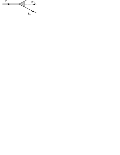
Figure 1: Graphical representation of the Light Front two-body wave function. Dash line corresponds to the spurion (see text).

Wave functions we deal with are Fock components of the state vector defined on the light-front plane $\omega\makebox[2.27626pt]{$\cdot$}x=0$. For a two-fermion system – shown graphically in Fig. 1 – it reads:

$${\mit\Phi}_{\sigma_{2}\sigma_{1}}={\mit\Phi}_{\sigma_{2}\sigma_{1}}(k_{1},k_{2},p,\omega\tau)$$ (1)

were $\sigma_{i}$ are the constituent angular momenta. The general form of the wave function is obtained by constructing all possible spin structures compatible with the quantum numbers of the state. The four-vector $\omega$ enters in the wave function on the same ground than the particles four-momenta, giving rise to a number of structures larger than in non relativistic dynamics. Each of them is mastered by a scalar function, denoted $f_{i}$ all through the paper, which can be interpreted as a wave function component on the spin space. The number N of such independent amplitudes simply follows from the dimension of the spin matrix forming the two-fermion wave function with total momentum $J$, i.e. $N={1\over 2}(2J+1)(2\sigma_{1}+1)(2\sigma_{2}+1)$ with a factor ${1\over 2}$ to take into account the parity conservation. In the case $\sigma_{1}=\sigma_{2}={1\over 2}$, it gives $N$=2 amplitudes for $J$=0 states and $N$=6 for $J$=1. These wave function components will be specified in the coming sections.

Since the Fock-space component is, by construction, the coefficient of the state vector decomposition in the creation operators basis: $a^{\dagger}_{\sigma_{2}}(\vec{k}_{2})a^{\dagger}_{\sigma_{1}}(\vec{k}_{1})|0\rangle$, the independent variables are the three-dimensional vectors ($\vec{k}_{1},\vec{k}_{2}$) and the particles energies are expressed through them. Consequently all four-momenta are on corresponding mass shells: $k_{1}^{2}=k_{2}^{2}=m^{2}$, $p^{2}=M^{2}$, $(\omega\tau)^{2}=0$ and satisfy the conservation law:

$$k_{1}+k_{2}=p+\omega\tau.$$ (2)

This equation generalizes the $(\perp,+)$-components conservation in the standard approach; the minus components are not constrained. In the light-front coordinates with $\omega=(1,0,0,-1)$, the only non-zero component of $\omega$ is $\omega_{-}=\omega_{0}-\omega_{z}=2$. The four-vector $\omega\tau$ just incorporates the non-vanishing difference $2\tau=k_{1-}+k_{2-}-p_{-}$. In this sense the ECLFD wave function is off energy shell. Since the four-momentum $\omega\tau$ enters in the wave function on equal ground with the particle momenta, we associate it for convenience with a fictitious particle – called spurion – showed in Fig. 1 by a dash line. We would like to emphasize however that the Fock space basis does not contain for all that any additional and unphysical degree of freedom. By spurion, we mean only the difference – proportional to $\omega$ – between non-conserved particle four-momenta in the off-energy-shell states.

It is convenient to introduce other kinematical variables, constructed from the initial four-momenta as follows:

$$\vec{k} = L^{-1}({\cal P})\vec{k}_{1}=\vec{k}_{1}-\frac{\vec{\cal P}}{\sqrt{{\cal P}^{2}}}\left[k_{10}-\frac{\vec{k}_{1}\makebox[2.27626pt]{$\cdot$}\vec{{\cal P}}}{\sqrt{{\cal P}^{2}}+{\cal P}_{0}}\right]$$ (3)

$$\vec{n} = \frac{L^{-1}({\cal P})\vec{\omega}}{\mid L^{-1}({\cal P})\vec{\omega}\mid}$$ (4)

where ${\cal P}=p+\omega\tau$, and $L^{-1}({\cal P})$ results from the Lorentz boost into the reference system where $\vec{\cal P}=0$. In these variables the wave function (1) is represented as:

$${\mit\Phi}_{\sigma_{2}\sigma_{1}}={\mit\Phi}_{\sigma_{2}\sigma_{1}}(\vec{k},\vec{n}).$$ (5)

Under rotations and Lorentz transformations of four-momenta $k_{1},k_{2},p,\omega\tau$, variables ($\vec{k},\vec{n}$) are only rotated, so the three-dimensional parametrization (5) is also explicitly covariant. In practice, instead of the formal transformations (3), it is enough to consider the wave function and the equation in the c.m. system where $\vec{\cal P}=\vec{k}_{1}+\vec{k}_{2}=0$ and set $\vec{k}_{1}=\vec{k}$, $\vec{k}_{2}=-\vec{k}$, $\vec{\omega}=\vec{n}|\vec{\omega}|$. Because of covariance, the result is the same as after transformation (3). Since $\vec{\omega}$ determines only the orientation of the light-front plane, the modulus $|\vec{\omega}|$ disappears from the wave functions and amplitudes. Note that in the c.m. system, the momentum $\vec{p}$ is not zero: $\vec{p}=-\vec{\omega}\tau$.

The light-front graph techniques is a covariant generalization of the old fashioned perturbation theory. The latter was developed by Kadyshevsky kadysh and adapted to the explicitly covariant version in VAK_76 ; CDKM_PR_98 .

The equation for the wave function is shown graphically in Fig.2.

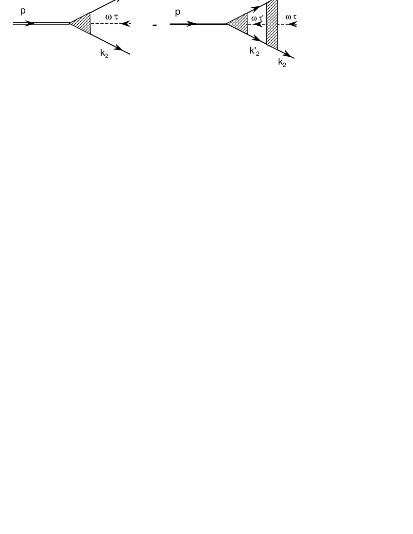
Figure 2: Equation for the two-body wave function.

It is the projection on the two-body sector of the general mass equation $P^{2}\phi=M^{2}\phi$. Its analytical form is obtained by applying the rules of the graph techniques to the diagrams in Fig. 2. In variables (3) this equations reads:

$$\left[4(\vec{k}\,^{2}+m^{2})-M^{2}\right]{\mit\Phi}_{\sigma_{2}\sigma_{1}}(\vec{k},\vec{n})=-\frac{m^{2}}{2\pi^{3}}\int\sum_{\sigma^{\prime}_{1}\sigma^{\prime}_{2}}K_{\sigma_{2}\sigma_{1}}^{\sigma^{\prime}_{2}\sigma^{\prime}_{1}}(\vec{k},\vec{k}\,^{\prime},\vec{n},M^{2}){\mit\Phi}_{\sigma^{\prime}_{2}\sigma^{\prime}_{1}}(\vec{k}\,^{\prime},\vec{n})\frac{d^{3}k^{\prime}}{\varepsilon_{k^{\prime}}}\ .$$ (6)

where $K_{\sigma_{2}\sigma_{1}}^{\sigma^{\prime}_{2}\sigma^{\prime}_{1}}(\vec{k},\vec{k}\,^{\prime},\vec{n},M^{2})$ is the interaction kernel. We detail in what follows the LFD one-boson exchange kernels corresponding to the interaction Lagrangians:

• Scalar (S):

  $${\cal L}^{int}=g_{s}\ \bar{\psi}\psi\phi^{(s)}$$ (7)

• Pseudoscalar (PS):

  $${\cal L}^{int}=i\ g_{ps}\ \bar{\psi}\gamma_{5}\psi\ \phi^{(ps)}$$ (8)

• Pseudovector (PV):

  $${\cal L}^{int}=-\frac{f_{pv}}{2m}\ \bar{\psi}\gamma^{\mu}\gamma_{5}\ \psi\ \partial_{\mu}\ \phi^{(ps)}$$ (9)

• Vector (V):

  $${\cal L}^{int}=\bar{\psi}[g_{v}\gamma^{\mu}\phi^{(v)}_{\mu}+{f_{t}\over 4m}\sigma^{\mu\nu}(\partial_{\mu}\phi^{(v)}_{\nu}-\partial_{\nu}\phi^{(v)}_{\mu})]\psi$$ (10)

  with

  $$\sigma^{\alpha^{\prime}\alpha}=\frac{i}{2}(\gamma^{\alpha^{\prime}}\gamma^{\alpha}-\gamma^{\alpha}\gamma^{\alpha^{\prime}}).$$

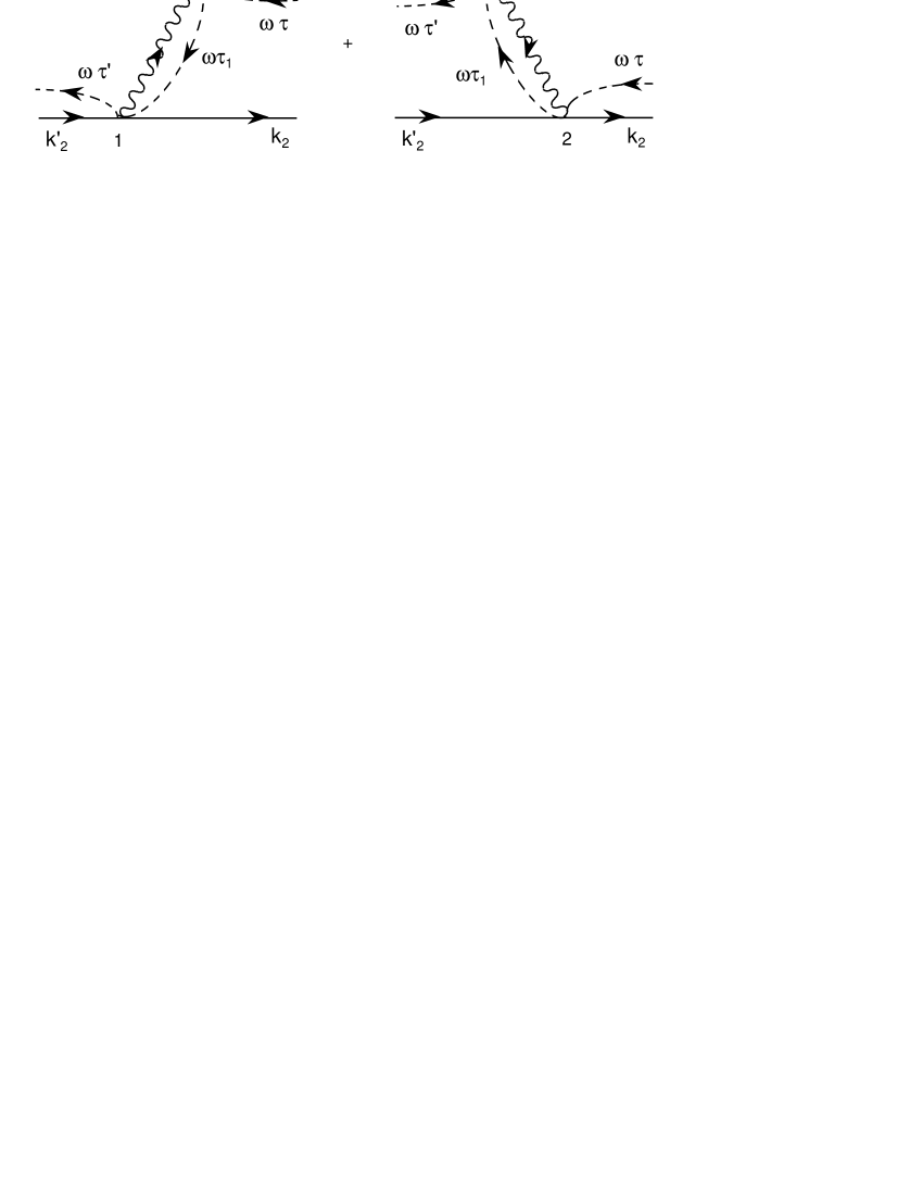
Figure 3: One boson exchange kernel.

The LFD ladder kernels have two contributions corresponding to the two time-ordered diagrams (in the light-front time) shown in Fig. 3. For S, PS and PV couplings they have the structure:

$$K^{\sigma^{\prime}_{2}\sigma^{\prime}_{1}}_{\sigma_{2}\sigma_{1}}(k_{1},k_{2},\omega\tau;k^{\prime}_{1},k^{\prime}_{2},\omega\tau^{\prime})=-\frac{1}{4m^{2}}\left[\bar{u}^{\sigma_{2}}(k_{2})O_{2}u^{\sigma^{\prime}_{2}}(k^{\prime}_{2})\right]\;\left[\bar{u}^{\sigma_{1}}(k_{1})O_{1}u^{\sigma^{\prime}_{1}}(k^{\prime}_{1})\right]\qquad\qquad$$

$$\times \left\{\frac{\theta\left(\omega\makebox[2.27626pt]{$\cdot$}(k^{\prime}_{1}-k_{1})\right)}{\mu^{2}-(k^{\prime}_{1}-k_{1})^{2}+2\tau^{\prime}\omega\makebox[2.27626pt]{$\cdot$}(k^{\prime}_{1}-k_{1})}\right.+\left.\frac{\theta\left(\omega\makebox[2.27626pt]{$\cdot$}(k_{1}-k^{\prime}_{1})\right)}{\mu^{2}-(k_{1}-k^{\prime}_{1})^{2}+2\tau\omega\makebox[2.27626pt]{$\cdot$}(k_{1}-k^{\prime}_{1})}\right\}.$$

For scalar exchange

$$O_{1}=O_{2}=g_{s},$$

for pseudoscalar

$$O_{1}=O_{2}=i\gamma_{5}g_{ps}$$

and for pseudovector

$$O_{1}=\left\{\begin{array}[]{ll}\left(1-\frac{\hat{\omega}\tau}{2m}\right)i\gamma_{5}f_{pv},&\mbox{if}\quad\omega\makebox[2.27626pt]{$\cdot$}(k_{1}-k^{\prime}_{1})>0\\ \left(1+\frac{\hat{\omega}\tau^{\prime}}{2m}\right)i\gamma_{5}f_{pv},&\mbox{if}\quad\omega\makebox[2.27626pt]{$\cdot$}(k_{1}-k^{\prime}_{1})<0\end{array}\right.$$

$$O_{2}=\left\{\begin{array}[]{ll}\left(1+\frac{\hat{\omega}\tau^{\prime}}{2m}\right)i\gamma_{5}f_{pv},&\mbox{if}\quad\omega\makebox[2.27626pt]{$\cdot$}(k_{1}-k^{\prime}_{1})>0\\ \left(1-\frac{\hat{\omega}\tau}{2m}\right)i\gamma_{5}f_{pv},&\mbox{if}\quad\omega\makebox[2.27626pt]{$\cdot$}(k_{1}-k^{\prime}_{1})<0\end{array}\right.$$

with:

$$\tau=\frac{4\varepsilon_{k}^{2}-M^{2}}{2\omega\makebox[2.27626pt]{$\cdot$}p},\quad\tau^{\prime}=\frac{4\varepsilon_{k^{\prime}}^{2}-M^{2}}{2\omega\makebox[2.27626pt]{$\cdot$}p}.$$

For values $\tau,\tau^{\prime}\neq 0$ the kernels are off energy shell. In this case the pseudoscalar and pseudovector kernels differ from each other but coincide on energy shell ($\tau=\tau^{\prime}=0$).

We use the notation $\hat{\omega}=\omega_{\mu}\gamma^{\mu}$. Writing the propagators in the center of mass variables, (II) gets the simpler form:

$$K^{\sigma^{\prime}_{2}\sigma^{\prime}_{1}}_{\sigma_{2}\sigma_{1}}=-\frac{1}{4m^{2}}\frac{1}{Q^{2}+\mu^{2}}\left[\bar{u}_{\sigma_{2}}(k_{2})O_{2}u_{\sigma^{\prime}_{2}}(k^{\prime}_{2})\right]\,\left[\bar{u}_{\sigma_{1}}(k_{1})O_{1}u_{\sigma^{\prime}_{1}}(k^{\prime}_{1})\right],$$ (12)

with

$$Q^{2} = (\vec{k}-\vec{k}^{\prime})^{2}-(\vec{k}\makebox[2.27626pt]{$\cdot$}\vec{n})(\vec{k}^{\prime}\makebox[2.27626pt]{$\cdot$}\vec{n})\frac{(\varepsilon_{k}-\varepsilon_{k^{\prime}})^{2}}{\varepsilon_{k}\varepsilon_{k^{\prime}}}+\left(\varepsilon_{k}^{2}+\varepsilon_{k^{\prime}}^{2}-\frac{1}{2}M^{2}\right)\left|\frac{\vec{k}\makebox[2.27626pt]{$\cdot$}\vec{n}}{\varepsilon_{k}}-\frac{\vec{k}^{\prime}\makebox[2.27626pt]{$\cdot$}\vec{n}}{\varepsilon_{k^{\prime}}}\right|$$ (13)

The kernel for the vector coupling is given by a contraction of terms similar to (12) with the tensor structures $L_{\alpha\beta}$. It reads

$$K^{\sigma^{\prime}_{2}\sigma^{\prime}_{1}}_{\sigma_{2}\sigma_{1}}=-\frac{1}{4m^{2}}\frac{1}{\mu^{2}+Q^{2}}L_{\alpha\beta}\left[\bar{u}(k_{1})O_{1}^{\alpha}u(k^{\prime}_{1})\right]\;\left[\bar{u}(k_{2})O_{2}^{\beta}u(k^{\prime}_{2})\right],$$ (14)

with

$$L_{\alpha\beta}=\left\{\begin{array}[]{ll}-g_{\alpha\beta}+{1\over\mu^{2}}(k_{1}-k^{\prime}_{1}-\omega\tau)_{\alpha}(k^{\prime}_{2}-k_{2}-\omega\tau^{\prime})_{\beta},&\mbox{if}\quad\omega\makebox[2.27626pt]{$\cdot$}(k_{1}-k^{\prime}_{1})>0\\ -g_{\alpha\beta}+{1\over\mu^{2}}(k^{\prime}_{1}-k_{1}-\omega\tau^{\prime})_{\alpha}(k_{2}-k^{\prime}_{2}-\omega\tau)_{\beta},&\mbox{if}\quad\omega\makebox[2.27626pt]{$\cdot$}(k_{1}-k^{\prime}_{1})<0\end{array}\right.$$ (15)

and vertex operators

$$O_{1}^{\alpha}=\left\{\begin{array}[]{ll}g_{v}\gamma^{\alpha}+\frac{\displaystyle{f_{t}}}{\displaystyle{2m}}\sigma^{\alpha^{\prime}\alpha}(-i)(k_{1}-k^{\prime}_{1}-\omega\tau)_{\alpha^{\prime}},&\mbox{if}\quad\omega\makebox[2.27626pt]{$\cdot$}(k_{1}-k^{\prime}_{1})>0\\ g_{v}\gamma^{\alpha}+\frac{\displaystyle{f_{t}}}{\displaystyle{2m}}\sigma^{\alpha^{\prime}\alpha}(i)(k^{\prime}_{1}-k_{1}-\omega\tau^{\prime})_{\alpha^{\prime}},&\mbox{if}\quad\omega\makebox[2.27626pt]{$\cdot$}(k_{1}-k^{\prime}_{1})<0\end{array}\right.$$ (16)

$$O_{2}^{\beta}=\left\{\begin{array}[]{ll}g_{v}\gamma^{\beta}+\frac{\displaystyle{f_{t}}}{\displaystyle{2m}}\sigma^{\beta^{\prime}\beta}(i)(k^{\prime}_{2}-k_{2}-\omega\tau^{\prime})_{\beta^{\prime}},&\mbox{if}\quad\omega\makebox[2.27626pt]{$\cdot$}(k_{1}-k^{\prime}_{1})>0\\ g_{v}\gamma^{\beta}+\frac{\displaystyle{f_{t}}}{\displaystyle{2m}}\sigma^{\beta^{\prime}\beta}(-i)(k_{2}-k^{\prime}_{2}-\omega\tau)_{\beta^{\prime}},&\mbox{if}\quad\omega\makebox[2.27626pt]{$\cdot$}(k_{1}-k^{\prime}_{1})<0\end{array}\right.$$ (17)

Hereafter we will not take into account the tensor coupling, that is we put $f_{t}=0$ and $O_{1}^{\alpha}=O_{2}^{\alpha}=g_{v}\gamma^{\alpha}$. In this case, vector kernel (14) simplifies into:

$$K^{\sigma^{\prime}_{2}\sigma^{\prime}_{1}}_{\sigma_{2}\sigma_{1}} = \frac{g_{v}^{2}}{4m^{2}}\frac{1}{\mu^{2}+Q^{2}}\left\{\left[\bar{u}(k_{1})\gamma^{\alpha}u(k^{\prime}_{1})\right]\;\left[\bar{u}(k_{2})\gamma_{\alpha}u(k^{\prime}_{2})\right]-\frac{\tau\tau^{\prime}}{\mu^{2}}\left[\bar{u}(k_{1})\hat{\omega}u(k^{\prime}_{1})\right]\;\left[\bar{u}(k_{2})\hat{\omega}u(k^{\prime}_{2})\right]\right\}$$ (18)

In the $\mu=0$ case, e.g. one-photon or one-gluon exchange kernels, the $L_{\alpha\beta}$ expressions depend on the gauge. Using the Feynman gauge, one has $L_{\alpha\beta}=-g_{\alpha\beta}$, i.e. the $\mu$-dependent terms on (15) and (18) are simply dropped out.

It will be often necessary to regularize the LFD kernels by means of vertex form factors. Unless explicit mention of the contrary we will take the form used in the Bonn model Bonn , i.e.

$$F(Q^{2})=\left({\Lambda^{2}-\mu^{2}\over\Lambda^{2}+Q^{2}}\right)^{n}$$ (19)

where $\Lambda$ and $n$ are parameters whose values depend on the coupling. Form factors appear in the kernels multiplying each of the vertex operators $O_{i}$. In the non relativistic limit, $Q^{2}\approx(\vec{k}-\vec{k}^{\prime})^{2}$ and $F$ is local in configuration space. This locality is however broken from the very beginning in LFD due to the $\vec{n}$-dependent terms on $Q^{2}$.

III Angular momentum

In LFD the construction of states with definite angular momentum is a delicate problem. Working in the explicitly covariant version, we have developed a method to overcome this difficulty. It will be explained in this section. In contrast to the equal-time approach, the LFD generators $J_{\rho\gamma}=J^{0}_{\rho\gamma}+J^{int}_{\rho\gamma}$ of four-dimensional rotations are not kinematical, but contain interaction in $J^{int}_{\rho\gamma}$. The interaction also enters in the angular momentum operator, i.e. the Pauli-Lubansky vector:

$$S_{\mu}=\frac{1}{2}\varepsilon_{\mu\nu\rho\gamma}P^{\nu}J^{\rho\gamma}.$$ (20)

Like the action of the Hamiltonian on the Schrödinger wave function is expressed through the time derivative

$$H^{int}\,\phi=i\partial_{t}\phi\ ,$$

the action of $J^{int}_{\rho\gamma}$ on the LFD state vector is expressed through derivatives with respect to the four-vector $\omega$ karm82 :

$$J^{int}_{\mu\nu}\,\phi(\omega)=L_{\mu\nu}(\omega)\phi(\omega)\ ,$$ (21)

where:

$$L_{\mu\nu}(\omega)=i\left(\omega_{\mu}\frac{\partial}{\partial\omega^{\nu}}-\omega_{\nu}\frac{\partial}{\partial\omega^{\mu}}\right)\ .$$ (22)

Equation (21) is called angular condition and can also be written in the form:

$$S_{\mu}\,\phi(\omega)=W_{\mu}\,\phi(\omega)$$ (23)

with

$$W_{\mu}=\frac{1}{2}\epsilon_{\mu\nu\rho\gamma}P^{\nu}M^{\rho\gamma}$$ (24)

and

$$M_{\mu\nu}=J^{0}_{\mu\nu}+L_{\mu\nu}(\omega).$$

$W_{\mu}$ is a kinematical Pauli-Lubansky vector. As far as the angular condition is satisfied, the dynamical Pauli-Lubansky vector $S_{\mu}$ can be replaced by the kinematical one $W_{\mu}$. The great benefit of doing so is that the problem of constructing angular momentum states with operator (24) becomes purely kinematical. In practice one rather prefers to start constructing states with definite angular momentum using $W_{\mu}$, and then take into account the restriction imposed by the angular condition (21).

It is worth noticing that without this condition, there is an ambiguity in defining the state vector with given angular momentum. This can be seen by introducing the operator:

$$\hat{A}^{2}=\left(\frac{W\makebox[2.27626pt]{$\cdot$}\omega}{P\makebox[2.27626pt]{$\cdot$}\omega}\right)^{2}.$$ (25)

It commutes with $P_{\mu}$ and $W_{\mu}$ and – taking $A^{2}$ instead of $A$ – with the parity operator. The state vector is then characterized not only by its mass $M^{2}$, momentum $p$, angular momentum $J$ – defined by means of (24) – and parity $\pi$ but also by $a$, square root of the $A^{2}$ eigenvalue:

$$\hat{A}^{2}\ \phi^{(a)}=a^{2}\ \phi^{(a)}\ .$$ (26)

For a total angular momentum $J$ there are $J+1$ eigenstates $\phi^{(a)}$. In principle one could imagine any of these eigenstates to be an acceptable solution. It turns out however that, except for $J=0$, none of these eigenstates can satisfy the angular condition (23). Indeed if $\phi(\omega)$ is an eigenstate of $A^{2}$, the right hand side of (23) – $W_{\mu}\phi(\omega)$ – is still an eigenstate of $A^{2}$ whereas this is not possible in its left hand side – $S_{\mu}\phi(\omega)$ – due to the non zero commutator $[S_{\mu},A^{2}]\neq 0$. What is then the state vector?

A solution of the angular condition – the only remaining equation to be fulfilled – is therefore provided by a linear combination of different eigenstates $\phi^{(a)}$:

$$\phi=\sum_{a=0}^{J}c_{a}\,\phi^{(a)}.$$ (27)

The coefficients $c_{a}$ can in principle be determined by inserting (27) into (21) or (23).

We would like to emphasize this result, which is, to our opinion, an important issue of Light-Front Dynamics. It tells us that the state vector is necessarily a superposition of different $A^{2}$ eigenstates. This conclusion does not depend on the approximation resulting from any eventual Fock-space truncation.

In an exact solution of the problem, i.e. with the generators satisfying the Poincaré algebra, the eigenstates $\phi^{(a)}$ are degenerate in mass and the superposition (27) is furthermore a solution of the mass equation (6). Indeed, as already noticed, $S_{\mu}\phi^{(a)}$ is not an eigenstate of $A^{2}$ but a superposition of different $A^{2}$ eigenstates. On the other hand, the commutation relation $[S_{\mu},P_{\nu}]=0$ implies $S_{\mu}\phi^{(a)}$ to have the same mass than $\phi^{(a)}$. This is possible only if the masses of different states $\phi^{(a)}$ are equal.

Due to the Fock-space truncation, or to some other kind of approximation, the Poincaré algebra is violated. The eigenstates $\phi^{(a)}$ are no longer degenerate and the solution (27), built with eigenstates of different mass, cannot satisfy equation (6). However, while this equation is an approximate one, the form (27) for the state vector remains valid. Each term in (32) is an exact solution of the truncated mass equation (6) with eigenvalue $M^{2}_{a}$. Their superposition satisfies no any mass equation but has the proper form of the non-truncated hamiltonian problem. The corresponding mass squared – at the same level of approximation – is given by:

$$M^{2}=\sum_{a=0}^{J}c_{a}^{2}M_{a}^{2}$$ (28)

The ensemble $(\phi,M)$ obtained that way, constitutes the solution of the problem compatible with the degree of approximation considered.

This formalism is translated to $J=1$ states in the two-body sector as follows. The interaction kernel $K(\vec{k}\,^{\prime},\vec{k},\vec{n},M)$ depends on scalar products of vectors $\vec{k}\,^{\prime},\vec{k},\vec{n}$ and also on scalar products with Pauli matrices: $\vec{k}\makebox[2.27626pt]{$\cdot$}\vec{\sigma}$, $\vec{k}\,^{\prime}\makebox[2.27626pt]{$\cdot$}\vec{\sigma}$, $\vec{n}\makebox[2.27626pt]{$\cdot$}\vec{\sigma}$. Therefore the total angular momentum operator constructed as

$$\vec{J}=-i[\vec{k}\times\partial_{\vec{k}}\,]-i[\vec{n}\times\partial_{\vec{n}}\,]+\vec{s}_{1}+\vec{s}_{2}\ ,$$ (29)

commutes with the kernel ($\vec{s}_{1,2}$ are the fermion spin operators). In the c.m. system this operator is proportional to the kinematical Pauli-Lubansky vector $\vec{W}$ given in (24). The solutions of equation (6) correspond to definite $J$ and $J_{z}$ eigenvalues of the operators $\vec{J}^{2},J_{z}$.

Since $A^{2}$ is applied to states with definite $p$, it has the form:

$$A^{2}=(\vec{n}\makebox[2.27626pt]{$\cdot$}\vec{J})^{2}.$$ (30)

$A^{2}$ commutes with the kernel $K$ since $\vec{J}$ commutes with $K$ and $\vec{n}$ is a parameter. It commutes also with $\vec{J}$ since $A$ is a scalar. Thus, like in the case of a full state vector (26), the truncated solutions in the two-body sector are also labelled by $a$:

$$A^{2}\;\vec{\psi}^{(a)}(\vec{k},\vec{n})=a^{2}\;\vec{\psi}^{(a)}(\vec{k},\vec{n}).$$ (31)

and the two-body wave function is a superposition of $A^{2}$ eigenstates $\vec{\psi}^{(a)}$ with different $a$ values:

$$\vec{\psi}(\vec{k},\vec{n})=c_{0}\;\vec{\psi}^{(0)}(\vec{k},\vec{n})+c_{1}\;\vec{\psi}^{(1)}(\vec{k},\vec{n}).$$ (32)

The mass equations determining the eigenstates $\vec{\psi}^{(a)}$ with different $a$ are decoupled; in particular, the $J=0$ state is determined by one single equation. We would like to comment here that the decoupling into subsystems takes place in any formulation of LFD, both in the explicitly covariant and in the standard one. However, in the latter approach it looks as a matter of art, whereas in ECLFD this splitting has transparent reasons. For example, in GHPSW_PRD47_93 the four equations system for the wave function components with angular momentum projection $m=0$ was split, by a proper transformation, in two subsystems with two equations each. In ECLFD this corresponds to the $a=0$ eigenstate of $J=0$ and $J=1$ states, each of them having two components.

Because the truncation of the Fock space, the states $\vec{\psi}^{(a)}$ are not degenerate. Their splitting was effectively calculated in case of scalar particles in CMP_PRC61_00 ; MCK_Heid_00 ; KCM_Taiw_01 for $J=1,2$ as a function of the coupling constant. It has been shown in CMP_PRC61_00 that this splitting indeed decreased when the interaction kernel incorporates larger number of particles in the intermediate states. However, the number of states taken into account in any practical calculation will be always very limited. The splitting, though decreased, will remain, specially for strongly bound systems like $q\bar{q}$ mesons. The problem of determining the state vector at a given level of approximation is thus not solved by this way. These are some of the reasons why, as explained before, our approach to deal with this problem follows a different philosophy. Despite the non degeneracy of $\vec{\psi}^{(a)}$, we search the physical two-body wave function in the form (32), the same as for the full state vector (27). The corresponding mass squared is given by:

$$M^{2}=c_{0}^{2}M_{0}^{2}+c_{1}^{2}M_{1}^{2}$$ (33)

where $M^{2}_{a}$ is the mass associated with $\vec{\psi}^{(a)}$. The $M^{2}$ value thus obtained is always between $M_{0}^{2}$ and $M_{1}^{2}$, where would be the exact solution.

To determine in practice coefficients $c_{a}$, we use a method proposed in MCK_Heid_00 ; KCM_Taiw_01 ; MMB_These_01 , without explicitly solving (21). It is based on the fact that, when the momentum $k\to 0$, the interaction part in (21) is irrelevant and the angular condition reads simply $L_{\mu\nu}\phi=0$. Thus, in this limit, $\vec{\psi}$ does not depend on the light-front direction $\vec{n}$ anymore. Such a requirement unambiguously determines the coefficients of the superposition. The method was applied to a model with scalar particles KCM_Taiw_01 and found to give very accurate results. The procedure will be detailed in section V and illustrated by numerical calculations in section VII.

IV $J=0$ states

The $J=0^{+}$ two-fermion wave function can be written in the form CK_NPA589_95 ; CDKM_PR_98 :

$${\mit\Phi}_{\sigma_{2}\sigma_{1}}(k_{1},k_{2},p,\omega\tau)=\sqrt{m}\overline{u}_{\sigma_{2}}(k_{2})\;\phi\;U_{c}\overline{u}_{\sigma_{1}}(k_{1}),$$ (34)

where

$$u_{\sigma}(k)=\sqrt{\varepsilon_{k}+m}\left(\begin{array}[]{c}1\\ \frac{\displaystyle\vec{\sigma}\makebox[2.27626pt]{$\cdot$}\vec{k}}{\displaystyle(\varepsilon_{k}+m)}\end{array}\right)w_{\sigma},$$ (35)

is the Dirac spinor normalized to $\bar{u}_{\sigma}u_{\sigma^{\prime}}=2m\delta_{\sigma\sigma^{\prime}}$, $w_{\sigma}$ the Pauli spinor normalized to $w^{\dagger}_{\sigma}w_{\sigma^{\prime}}=\delta_{\sigma\sigma^{\prime}}$ and $\varepsilon_{k}=\sqrt{\vec{k}\,^{2}+m^{2}}$. $U_{c}=\gamma^{2}\gamma^{0}$ is the charge conjugation matrix. In its turn, $\phi$ is written as a superposition of two independent spin structures $S_{i}$

$$S_{1} = \frac{1}{2\sqrt{2}\varepsilon_{k}}\gamma_{5}$$ (36)

$$S_{2} = \frac{\varepsilon_{k}}{2\sqrt{2}mk\sin\theta}\left(\frac{2m}{\omega\makebox[2.27626pt]{$\cdot$}p}\hat{\omega}-\frac{m^{2}}{\varepsilon_{k}^{2}}\right)\gamma_{5}$$

whose coefficients $f_{i}$, scalar functions depending on variables $(k,\cos\theta=\vec{n}\makebox[2.27626pt]{$\cdot$}\vec{k}/k)$, are the wave function components in the spin-space:

$$\phi=f_{1}S_{1}+f_{2}S_{2},$$ (37)

The existence of one additional component with respect to the non-relativistic theory is due to the $\hat{\omega}=\omega_{\mu}\gamma^{\mu}$ term. The number of independent amplitudes determining the wave function is however the same, whatever will be the LFD version used. We have shown in a preceding work MCK_PRD_01 that the $J^{\pi}=0^{+}$ state we are considering is strictly equivalent in the standard approach to the $(1+,2-)$ one GHPSW_PRD47_93 which is described also by two components $\Phi^{1+},\Phi^{2-}$.

In the reference system where $\vec{k}_{1}+\vec{k}_{2}=0$ the wave function (34) takes the form:

$${\mit\Phi}_{\sigma_{2}\sigma_{1}}=\sqrt{m}w_{\sigma_{2}}^{\dagger}\psi(\vec{k},\vec{n})w_{\sigma_{1}}^{\dagger}$$ (38)

with

$$\psi(\vec{k},\vec{n})=\frac{1}{\sqrt{2}}\left(f_{1}+\frac{i\vec{\sigma}\makebox[2.27626pt]{$\cdot$}[\vec{k}\times\vec{n}]}{k\,\sin\theta}f_{2}\right)\sigma_{y},$$ (39)

The definition of the components themselves is to some extent arbitrary, as are arbitrary the choices of structures (36). Our choice (36) is justified by the clear separation of $\vec{n}$-independent and dependent terms it induces in the wave function (39).

The normalization condition reads:

$$\frac{1}{(2\pi)^{3}}\sum_{\sigma_{2}\sigma_{1}}\int\left|{\mit\Phi}_{\sigma_{2}\sigma_{1}}\right|^{2}{d^{3}k\over\varepsilon_{k}} = {m\over(2\pi)^{3}}\int Tr\{\bar{\phi}(\hat{k}_{2}+m)\phi(\hat{k}_{1}-m)\}{d^{3}k\over\varepsilon_{k}}$$ (40)

$$= {m\over(2\pi)^{3}}\int Tr\{\psi^{{\dagger}}(\vec{k},\vec{n})\psi(\vec{k},\vec{n})\}{d^{3}k\over\varepsilon_{k}}={m\over(2\pi)^{3}}\int(f_{1}^{2}+f_{2}^{2}){d^{3}k\over\varepsilon_{k}}=1,$$

where we denote $\bar{\phi}=\gamma_{0}\phi^{\dagger}\gamma_{0}$. The spin structures $S_{i}$ introduced in (36) are orthonormalized relative to the trace:

$$Tr\{\bar{S}_{i}(\hat{k}_{2}+m)S_{j}(\hat{k}_{1}-m)\}=\delta_{ij},$$ (41)

where $\bar{S}_{i}=\gamma_{0}S_{i}^{\dagger}\gamma_{0}$, that is:

$$\bar{S}_{1} = -\frac{1}{2\sqrt{2}\varepsilon_{k}}\gamma_{5}$$ (42)

$$\bar{S}_{2} = -\frac{\varepsilon_{k}}{2\sqrt{2}mk\sin\theta}\gamma_{5}\left(\frac{2m\hat{\omega}}{\omega\makebox[2.27626pt]{$\cdot$}p}-\frac{m^{2}}{\varepsilon_{k}^{2}}\right)$$ (43)

Substituting in (6) the wave function (34), multiplying it on left by $u(k_{2})$, on right by $u(k_{1})$ and using relation $\sum_{\sigma}u^{\sigma}(k)\bar{u}^{\sigma}(k)=\hat{k}+m$, we find:

$$[4(\vec{k}\,^{2}+m^{2})-M^{2}]\;(\hat{k}_{2}+m)\phi(\hat{k}_{1}-m)$$ (44)

$$=-\frac{m^{2}}{2\pi^{3}}\int\frac{1}{4m^{2}(Q^{2}+\mu^{2})}(\hat{k}_{2}+m)O_{2}(\hat{k}^{\prime}_{2}+m)\phi^{\prime}(\hat{k}^{\prime}_{1}-m)\tilde{O}_{1}(\hat{k}_{1}-m)\frac{d^{3}k^{\prime}}{\varepsilon_{k^{\prime}}}$$

with $\tilde{O}=U_{c}O^{t}U_{c}$. Replacing here $\phi$ by its decomposition (37), multiplying equation (44) by $\bar{S}_{i}$ and using the orthogonality relations (41), we end up with a two-dimensional integral equations system for components $f_{i}$:

$$[4(\vec{k}\,^{2}+m^{2})-M^{2}]\;f_{i}(k,\theta)=-\frac{m^{2}}{2\pi^{3}}\sum_{j=1,2}\int K_{ij}(k,\theta;k^{\prime},\theta^{\prime})f_{j}(k^{\prime},\theta^{\prime})\frac{d^{3}k^{\prime}}{\varepsilon_{k^{\prime}}},$$ (45)

Its solution will directly provide the mass of the $J^{\pi}=0^{+}$ state.

Kernels $K_{ij}$ appearing in (45) result from integrating kernels $\kappa_{ij}$ over the azimuthal angle $\varphi$:

$$K_{ij} = {1\over m^{2}\varepsilon_{k}\varepsilon_{k^{\prime}}}\int_{0}^{2\pi}{\kappa_{ij}\over Q^{2}+\mu^{2}}\;{d\varphi^{\prime}\over 2\pi},$$ (46)

with $Q^{2}$ defined in (13). For S, PS and PV couplings $\tilde{O}_{1}=U_{c}O^{t}_{1}U_{c}=O_{1}$ and $\kappa_{ij}$ are given by

$$\kappa_{ij} = {1\over 4}\varepsilon_{k}\varepsilon_{k}^{\prime}Tr\left[\bar{S}_{i}(\hat{k}_{2}+m)O_{2}(\hat{k^{\prime}}_{2}+m)S^{\prime}_{j}(\hat{k^{\prime}}_{1}-m)O_{1}(\hat{k}_{1}-m)\right]$$ (47)

We denote by $S^{\prime}_{j}$ the quantities (36) as a function of primed arguments. For vector exchange:

$$\kappa_{ij}=-\frac{1}{4}\varepsilon_{k}\varepsilon_{k}^{\prime}L_{\alpha\beta}Tr\left[\bar{S}_{i}(\hat{k}_{2}+m)O_{2}^{\alpha}(\hat{k^{\prime}}_{2}+m)S^{\prime}_{j}(\hat{k^{\prime}}_{1}-m)O_{1}^{\beta}(\hat{k}_{1}-m)\right],$$ (48)

Tensor $L_{\alpha\beta}$ is defined in (15) and we have taken into account that for V coupling $\tilde{O}_{1}=U_{c}O^{t}_{1}U_{c}=-O_{1}$. The analytic expressions of $\kappa_{ij}$ for S, PS, PV and V exchanges are given in appendix A.

One would remark that we have kept, for convenience, a three-dimensional volume element in equation (45) despite the fact that kernels $K_{ij}$ as well as amplitudes $f_{j}$ are independent of variable $\varphi^{\prime}$.

V $J=1$ states

In a similar way than in (34), the $J=1^{+}$ two-fermion wave function can be written in the form VAK_81 ; CK_NPA581_95 :

$${\mit\Phi}^{\lambda}_{\sigma_{2}\sigma_{1}}(k_{1},k_{2},p,\omega\tau)=\sqrt{m}\;e_{\mu}(p,\lambda)\;\bar{u}^{\sigma_{2}}(k_{2})\;\phi^{\mu}\;U_{c}\bar{u}^{\sigma_{1}}(k_{1})\ ,$$ (49)

where $e_{\mu}(p,\lambda)$ is the polarization vector. $\phi^{\mu}$ develops over the six spin structures

$$S_{1\mu}=\frac{(k_{1}-k_{2})^{\mu}}{2m^{2}},\quad S_{2\mu}=\frac{1}{m}\gamma^{\mu},\quad S_{3\mu}=\frac{\omega^{\mu}}{\omega\makebox[2.27626pt]{$\cdot$}p},\quad S_{4\mu}=\frac{(k_{1}-k_{2})^{\mu}\hat{\omega}}{2m\omega\makebox[2.27626pt]{$\cdot$}p},$$

$$S_{5\mu}=-\frac{i}{m^{2}\omega\makebox[2.27626pt]{$\cdot$}p}\gamma_{5}\epsilon^{\mu\nu\rho\gamma}k_{1\nu}k_{2\rho}\omega_{\gamma},\quad S_{6\mu}=\frac{m\omega^{\mu}\hat{\omega}}{(\omega\makebox[2.27626pt]{$\cdot$}p)^{2}}$$ (50)

with components $\varphi_{i}$, invariant functions depending on the same scalar variables than for $J=0$,

$$\phi^{\mu}=\varphi_{1}S_{1\mu}+\varphi_{2}S_{2\mu}+\varphi_{3}S_{3\mu}+\varphi_{4}S_{4\mu}+\varphi_{5}S_{5\mu}+\varphi_{6}S_{6\mu}\ .$$ (51)

In the reference system $\vec{k}_{1}+\vec{k}_{2}=0$ this wave function takes the form:

$$\vec{\mit\Psi}_{\sigma_{2}\sigma_{1}}(\vec{k},\vec{n})=\sqrt{m}w^{\dagger}_{\sigma_{2}}\vec{\psi}(\vec{k},\vec{n})\sigma_{y}w^{\dagger}_{\sigma_{1}}\ ,$$ (52)

with

$$\vec{\psi}(\vec{k},\vec{n}) = f_{1}\frac{1}{\sqrt{2}}\vec{\sigma}+f_{2}\frac{1}{2}(\frac{3\vec{k}(\vec{k}\makebox[2.27626pt]{$\cdot$}\vec{\sigma})}{\vec{k}^{2}}-\vec{\sigma})+f_{3}\frac{1}{2}(3\vec{n}(\vec{n}\makebox[2.27626pt]{$\cdot$}\vec{\sigma})-\vec{\sigma})$$ (53)

$$+ f_{4}\frac{1}{2k}(3\vec{k}(\vec{n}\makebox[2.27626pt]{$\cdot$}\vec{\sigma})+3\vec{n}(\vec{k}\makebox[2.27626pt]{$\cdot$}\vec{\sigma})-2(\vec{k}\makebox[2.27626pt]{$\cdot$}\vec{n})\vec{\sigma})+f_{5}\sqrt{\frac{3}{2}}\frac{i}{k}[\vec{k}\times\vec{n}]+f_{6}\frac{\sqrt{3}}{2k}(\vec{n}(\vec{k}\makebox[2.27626pt]{$\cdot$}\vec{\sigma})-\vec{k}(\vec{n}\makebox[2.27626pt]{$\cdot$}\vec{\sigma}))\ .$$

Contrary to the $J=0$ case, components $f_{i}$ appearing in (53) are not the same than $\varphi_{i}$ from (51). Their relation is given in Appendix B. Components $f_{3,4,5,6}$, driving $\vec{n}$-dependent spin structures, are of relativistic origin and are absent in a non relativistic approach.

As explained in section III, the system of equations determining the six components $f_{i}$ is split in two subsystems, corresponding to the eigenvalues $a=0,1$ of $\hat{A}^{2}$ (30). Like for the $J=0$ wave function, the $J=1,a=0$ eigenstate is determined by two components whereas the remaining four correspond to $J=1,a=1$. We would like to notice that the total number of components as well as the dimension of decoupled subsystems (2+4) coincides with what is found in the standard approach GHPSW_PRD47_93 .

The components determining the eigenstates $\vec{\psi}^{(a)}$ of $A^{2}$ will be respectively denote by $g_{i=1,2}^{(a=0)}$ and $g_{i=1,2,3,4}^{(a=1)}$. They are indeed different from the $f_{i}$ appearing in the wave function (53) though $g$’s fully determine $f$’s by linear combinations. In view of constructing the superposition (32) it is convenient to represent the eigenfunctions $\vec{\psi}^{(a)}$ in the form (53). Only some of the six $f_{i}^{(a)}$ involved components will be independent – two for the $a=0$ state and four for $a=1$ – but this way of doing will facilitate further analysis.

In the two coming subsections we will explicitly construct the eigenfunctions $\vec{\psi}^{(a)}$ of the kinematical operator $A^{2}$, obtain the corresponding mass equation (6) in terms of $g_{i}^{(a)}$ and relate them with components $f_{i}^{(a)}$ defined in (53).

V.1 $a=0$

One can check from equation (31) that $\vec{\psi}^{(0)}$ is parallel to $\vec{n}$, i.e. it satisfies $\vec{\psi}^{(0)}=\vec{n}(\vec{n}\makebox[2.27626pt]{$\cdot$}\vec{\psi}^{(0)})$, and has the following general decomposition:

$$\vec{\psi}^{(0)}(\vec{k},\vec{n})=\sqrt{\frac{3}{2}}\left\{g^{(0)}_{1}{\vec{\sigma}\makebox[2.27626pt]{$\cdot$}\vec{k}\over k}+g^{(0)}_{2}\frac{\vec{\sigma}\makebox[2.27626pt]{$\cdot$}(\vec{k}\cos\theta-k\vec{n})}{k\,\sin\theta}\right\}\vec{n},$$ (54)

It can be written in the form (53) by defining the $f^{(0)}_{i}$ components

$$f^{(0)}_{1} = \frac{1}{\sqrt{3}}\cos\theta g^{(0)}_{1}-\frac{1}{\sqrt{3}}\sin\theta g^{(0)}_{2}$$ (55)

$$f^{(0)}_{2} = 0$$ (56)

$$f^{(0)}_{3} = -\frac{\sqrt{2}}{\sqrt{3}\sin\theta}g^{(0)}_{2}$$ (57)

$$f^{(0)}_{4} = \frac{1}{\sqrt{6}}g^{(0)}_{1}+\frac{1}{\sqrt{6}}\cot\theta g^{(0)}_{2}$$ (58)

$$f^{(0)}_{5} = =0$$ (59)

$$f^{(0)}_{6} = \frac{1}{\sqrt{2}}g^{(0)}_{1}+\frac{1}{\sqrt{2}}\cot\theta g^{(0)}_{2}.$$ (60)

that is four non-zero components, with only two of them being independent. It can also be represented in a four-dimensional form similar to (51)

$$\phi^{(0)}_{\mu}=f^{(0)}_{1}S^{(0)}_{1\mu}+f^{(0)}_{2}S^{(0)}_{2\mu}.$$ (61)

by introducing the spin structures $S^{(0)}_{i\mu}$:

$$S^{(0)}_{1\mu} = \frac{\sqrt{3}M}{2\sqrt{2}k}S_{3\mu},$$ (62)

$$S^{(0)}_{2\mu} = \frac{\sqrt{3}M}{m\sqrt{2}\sin\theta}\left(\frac{m^{2}\cos\theta}{2\varepsilon_{k}k}S_{3\mu}+S_{6\mu}\right),$$ (63)

with $S_{i\mu}$ defined in (V).

The normalization condition is

$$\frac{1}{3(2\pi)^{3}}\sum_{\lambda\sigma_{2}\sigma_{1}}\int\left|{\mit\Phi}^{\lambda}_{\sigma_{2}\sigma_{1}}\right|^{2}{d^{3}k\over\varepsilon_{k}}={m\over(2\pi)^{3}}\int\Pi^{\mu\nu}Tr\{\phi^{(0)}_{\mu}(\hat{k}_{2}+m)\phi^{(0)}_{\nu}(\hat{k}_{1}-m)\}{d^{3}k\over\varepsilon_{k}}$$

$$= {m\over 3(2\pi)^{3}}\int Tr\{\vec{\psi}^{(0){\dagger}}(\vec{k},\vec{n})\vec{\psi}^{(0)}(\vec{k},\vec{n})\}{d^{3}k\over\varepsilon_{k}}={m\over(2\pi)^{3}}\int\left[(g^{(0)}_{1})^{2}+(g^{(0)}_{2})^{2}\right]{d^{3}k\over\varepsilon_{k}}=1.$$

with

$$\Pi^{\mu\nu}=\frac{1}{3}\sum_{\lambda}e^{\mu*}(p,\lambda)e^{\nu}(p,\lambda)=\frac{1}{3}\left(\frac{p^{\mu}p^{\nu}}{M^{2}}-g^{\mu\nu}\right).$$ (65)

The spin structures $S^{(0)}_{i\mu}$ are orthonormalized relative to the trace operation in (V.1) (cf. eq. (41)):

$$\Pi^{\mu\nu}Tr\{\bar{S}^{(0)}_{i\mu}(\hat{k}_{2}+m)S^{(0)}_{j\nu}(\hat{k}_{1}-m)\}=\delta_{ij}.$$ (66)

Note that $\bar{S}^{(0)}_{i\mu}=\gamma_{0}S^{(0)\dagger}_{i\mu}\gamma_{0}=S^{(0)}_{i\mu}$. Similarly to equation (44) we get:

$$\left[4(\vec{k}\,^{2}+m^{2})-M^{2}\right](\hat{k}_{2}+m)\phi^{(0)}_{\mu}(\hat{k}_{1}-m)$$ (67)

$$=-\frac{m^{2}}{2\pi^{3}}\int\frac{g^{2}}{4m^{2}(Q^{2}+\mu^{2})}(\hat{k}_{2}+m)O_{2}(\hat{k}^{\prime}_{2}+m)\phi^{\prime(0)}_{\mu}(\hat{k}^{\prime}_{1}-m)\tilde{O}_{1}(\hat{k}_{1}-m)\frac{d^{3}k^{\prime}}{\varepsilon_{k^{\prime}}}.$$

In order to obtain the system of equations for components $g^{(0)}_{i}$, we multiply equation (67) by $\Pi^{\mu\nu}$ and $S^{(0)}_{i\nu}$. Taking the trace and using the orthogonality condition (66) we obtain the system of equations:

$$\left[4(\vec{k}\,^{2}+m^{2})-M^{2}\right]g^{(0)}_{i}(\vec{k},\vec{n})=-\frac{m^{2}}{2\pi^{3}}\int\sum_{j=1}^{2}K^{(0)}_{ij}(\vec{k},\vec{k}\,^{\prime},\vec{n})g^{(0)}_{j}(\vec{k}\,^{\prime},\vec{n})\frac{d^{3}k^{\prime}}{\varepsilon_{k^{\prime}}}.$$ (68)

which provides the mass of the $J=1,a=0$ state. They have the same form than (45), with kernels $K^{(0)}_{ij}$ given in terms of $\kappa^{(0)}_{ij}$ integrated over the azimuthal angle $\varphi^{\prime}$:

$$K^{(0)}_{ij} = \frac{1}{m^{2}\varepsilon_{k}\varepsilon_{k^{\prime}}}\int_{0}^{2\pi}{\kappa^{(0)}_{ij}\over Q^{2}+\mu^{2}}{d\varphi^{\prime}\over 2\pi}.$$ (69)

For S, PS and PV couplings they read

$$\kappa^{(0)}_{ij}={1\over 4}\varepsilon_{k}\varepsilon_{k}^{\prime}\Pi^{\mu\nu}Tr\left[S^{(0)}_{i\mu}(\hat{k}_{2}+m)O_{2}(\hat{k^{\prime}}_{2}+m)\;S^{\prime(0)}_{j\nu}\;(\hat{k^{\prime}}_{1}-m)\;\tilde{O}_{1}(\hat{k}_{1}-m)\right]$$ (70)

where $S^{\prime(0)}_{j\nu}$ denotes (62) with primed arguments. For vector exchange

$$\kappa_{ij}^{(0)}=-\frac{1}{4}\varepsilon_{k}\varepsilon_{k}^{\prime}\Pi^{\nu\mu}L_{\alpha\beta}Tr\left[S^{(0)}_{i\nu}(\hat{k}_{2}+m)O_{2}^{\alpha}(\hat{k}^{\prime}_{2}+m){S^{\prime}}^{(0)}_{j\mu}(\hat{k}^{\prime}_{1}-m)O_{1}^{\beta}(\hat{k}_{1}-m)\right].$$ (71)

Tensors $L_{\alpha\beta}$ and $\Pi^{\nu\mu}$ are defined in (15) and (65). The analytic expressions of $\kappa_{ij}^{(0)}$ for S, PS, PV and V ($f_{t}=0$) exchanges are given in appendix A.

V.2 $a=1$

It follows also from (31) that $\vec{\psi}^{(1)}$, the $A^{2}$ eigenfunction corresponding to $a=1$, is orthogonal to $\vec{n}$, i.e. satisfies $\vec{n}\makebox[2.27626pt]{$\cdot$}\vec{\psi}^{(1)}=0$. To fulfill this condition, it is convenient to introduce two vectors ($\hat{\vec{k}}_{\perp},\vec{\sigma}_{\perp}$) orthogonal to $\vec{n}$:

$$\hat{\vec{k}}_{\perp} = \frac{\hat{\vec{k}}-\cos\theta\vec{n}}{\sin\theta}$$

$$\vec{\sigma}_{\perp} = \vec{\sigma}-(\vec{n}\makebox[2.27626pt]{$\cdot$}\vec{\sigma})\vec{n}.$$

with $\hat{\vec{k}}=\vec{k}/k$ and $\mid\hat{\vec{k}}_{\perp}\mid=1$. Function $\vec{\psi}^{(1)}$ obtains then the decomposition, analogous of (54),

$$\vec{\psi}^{(1)}(\vec{k},\vec{n})=g^{(1)}_{1}\frac{\sqrt{3}}{2}\vec{\sigma}_{\perp}+g^{(1)}_{2}\frac{\sqrt{3}}{2}\left(2\hat{\vec{k}}_{\perp}(\hat{\vec{k}}_{\perp}\makebox[2.27626pt]{$\cdot$}\vec{\sigma}_{\perp})-\vec{\sigma}_{\perp}\right)+g^{(1)}_{3}\sqrt{\frac{3}{2}}\hat{\vec{k}}_{\perp}(\vec{\sigma}\makebox[2.27626pt]{$\cdot$}\vec{n})+g^{(1)}_{4}\sqrt{\frac{3}{2}}i[\hat{\vec{k}}\times\vec{n}]$$ (72)

in terms of the four scalar amplitudes $g^{(1)}_{i}$. It can also be represented in the form (53) by defining components $f^{(1)}_{i}$

$$f^{(1)}_{1} = \sqrt{\frac{2}{3}}g^{(1)}_{1},$$ (73)

$$f^{(1)}_{2} = \frac{2}{\sqrt{3}\sin^{2}\theta}g^{(1)}_{2},$$ (74)

$$f^{(1)}_{3} = -\frac{1}{\sqrt{3}}g^{(1)}_{1}+\frac{(1+\cos^{2}\theta)}{\sqrt{3}\sin^{2}\theta}g^{(1)}_{2}-\frac{\sqrt{2}}{\sqrt{3}}\cot\theta g^{(1)}_{3},$$ (75)

$$f^{(1)}_{4} = -\frac{2\sqrt{3}\cos\theta}{3\sin^{2}\theta}g^{(1)}_{2}+\frac{1}{\sqrt{6}\sin\theta}g^{(1)}_{3},$$ (76)

$$f^{(1)}_{5} = \frac{1}{\sin\theta}g^{(1)}_{4},$$ (77)

$$f^{(1)}_{6} = -\frac{1}{\sqrt{2}\sin\theta}g^{(1)}_{3}$$ (78)

and in the four-dimensional form $\phi^{(1)}_{\mu}$ similar to (52):

$$\phi^{(1)}_{\mu}=g^{(1)}_{1}S^{(1)}_{1\mu}+g^{(1)}_{2}S^{(1)}_{2\mu}+g^{(1)}_{3}S^{(1)}_{3\mu}+g^{(1)}_{4}S^{(1)}_{4\mu}.$$ (79)

The four spin structures $S^{(1)}_{j\mu}$ are orthonormalized according to (66) and read:

$$S^{(1)}_{i\mu}=\sum_{j}h_{ij}S_{j\mu},\quad i=1,\ldots,4;\;j=1,\ldots,6,$$ (80)

with $S_{j\mu}$ defined in (V) and $h_{ij}$ coefficients given in appendix B. The normalization condition in terms of $\phi^{(1)}_{\mu}$ and $\vec{\psi}^{(1)}$ exactly coincides with (V.1). In terms of components $g^{(1)}_{i}$ it becomes:

$${m\over(2\pi)^{3}}\int\left[(g^{(1)}_{1})^{2}+(g^{(1)}_{2})^{2}+(g^{(1)}_{3})^{2}+(g^{(1)}_{4})^{2}\right]{d^{3}k\over\varepsilon_{k}}=1.$$ (81)

The system of equations for the scalar functions $g^{(1)}_{i}$ is obtained similarly to (68) and reads

$$\left[4(\vec{k}\,^{2}+m^{2})-M^{2}\right]g^{(1)}_{i}(\vec{k},\vec{n})=-\frac{m^{2}}{2\pi^{3}}\int\sum_{j=1}^{4}K^{(1)}_{ij}(\vec{k},\vec{k}\,^{\prime},\vec{n})g^{(1)}_{j}(\vec{k}\,^{\prime},\vec{n})\frac{d^{3}k^{\prime}}{\varepsilon_{k^{\prime}}}.$$ (82)

It is the mass equation of the $J=1,a=1$ states. Kernels $K^{(1)}_{ij}$ are calculated in a way similar than (69). The corresponding $\kappa_{ij}^{(1)}$ are obtained with the replacement $S^{(0)}_{i\mu}\rightarrow S^{(1)}_{i\mu}$ in (70) and (71). Their analytic expressions for S and PS exchanges are given in appendix A.

V.3 Physical solution

The solutions $\vec{\psi}^{(a)}$ constructed in the preceding sections, although being exact eigenstates of the truncated Hamiltonian, are only auxiliary. As explained in section III, the solution satisfying the angular condition (21) is given by the superposition (32) of states with different $a$. The coefficients $c_{a}$ of the superposition can be obtained by solving the angular condition in the truncated Fock space. We will show in what follows that they can alternatively be determined by imposing the independence of the wave function on the light-front vector $\vec{n}$ at $k=0$.

In order to do that, it is convenient to write down $\vec{\psi}^{(a)}$ in the form (53) with the components $f^{(a)}_{i}$ given by equations (55) and (73). Written in term of $f$’s the superposition (32) reads

$$f_{i}=c_{0}f^{(0)}_{i}+c_{1}f^{(1)}_{i}.$$ (83)

The condition that $\vec{\psi}(\vec{k}=0,\vec{n})$ does not depend on $\vec{n}$ becomes:

$$\partial_{\theta}f_{i}(k=0,\theta) \equiv 0\qquad i=1,2$$ (84)

$$f_{j}(k=0,\theta) \equiv 0\qquad j=3,4,5,6.$$ (85)

Let us show that there exists two coefficients $c_{a}$, normalized to $c_{0}^{2}+c_{1}^{2}=1$, satisfying the above six equations. They are determined by the only values at $k=0$ of the first components $g^{(a)}_{1}$.

To this aim, we consider the behavior of $f^{(a)}_{i}(k,z)$ in the $k\to 0$ limit. The components in front of structures involving the unit vector $\hat{\vec{k}}$ are $f^{(a)}_{2,4,5,6}$. By construction, they must vanish at $k=0$, i.e. satisfy:

$$f^{(a)}_{2,4,5,6}(k=0,\theta)\equiv 0\qquad a=0,1.$$ (86)

Concerning $a=0$ states, this condition is trivially satisfied by $f^{(0)}_{2,5}$ since from (55), they are identically zero whereas $f^{(0)}_{4,6}$ will satisfy (86) if:

$$g^{(0)}_{1}(k=0,\theta) = +b_{0}\cos\theta,$$ (87)

$$g^{(0)}_{2}(k=0,\theta) = -b_{0}\sin\theta,$$

$b_{0}$ being a priori an arbitrary function of $\theta$ which later on will be shown to be constant. The only components which are non zero at $k=0$ are $f^{(0)}_{1,3}$. Inserting the values (87) in (55) we find:

$$f^{(0)}_{1}(0,\theta) = \frac{1}{\sqrt{3}}\cos\theta g^{(0)}_{1}(0,\theta)-\frac{1}{\sqrt{3}}\sin\theta g^{(0)}_{2}(0,\theta)=\frac{1}{\sqrt{3}}b_{0}$$

$$f^{(0)}_{3}(0,\theta) = -\frac{\sqrt{2}}{\sqrt{3}\sin\theta}g^{(0)}_{2}(0,\theta)=\sqrt{\frac{2}{3}}b_{0}.$$

Concerning $a=1$ solutions, determined by four independent components $g^{(1)}_{i}$, we see from (73) that condition (86) implies $g^{(1)}_{2,3,4}(0,\theta)\equiv 0$. The only non-vanishing component at $k=0$ is thus $g^{(1)}_{1}$ and we will denote by $b_{1}$ its value:

$$g^{(1)}_{1}(0,\theta)=b_{1}.$$ (88)

By inserting this values in (73) we get:

$$f_{1}^{(1)}(0,\theta) = \sqrt{\frac{2}{3}}g_{1}^{(1)}(0,\theta)=\sqrt{\frac{2}{3}}b_{1},$$

$$f^{(1)}_{3}(0,\theta) = -\frac{1}{\sqrt{3}}g^{(1)}_{1}(0,\theta)+\frac{(1+\cos^{2}\theta)}{\sqrt{3}\sin^{2}\theta}g^{(1)}_{2}(0,\theta)-\frac{\sqrt{2}}{\sqrt{3}}\cot\theta g^{(1)}_{3}(0,\theta)=-\frac{1}{\sqrt{3}}b_{1}.$$

Components $f^{(0)}_{3}$ and $f^{(1)}_{3}$ are the only $\vec{n}$-dependent structures which gives non-zero contributions at $k=0$ in the corresponding wave functions $\vec{\psi}^{(0)}$ and $\vec{\psi}^{(1)}$. These contributions must cancel in the physical wave function $\vec{\psi}$, what gives the relation

$$f_{3}(0,\theta)=c_{0}\,f^{(0)}_{3}(0,\theta)+c_{1}\,f^{(1)}_{3}(0,\theta)=c_{0}\sqrt{\frac{2}{3}}b_{0}-c_{1}\frac{1}{\sqrt{3}}b_{1}=0$$

This relation, together with the normalization condition $c_{0}^{2}+c_{1}^{2}=1$, allows us to determine the coefficients $c_{a}$ of the superposition (32). They read:

$$c_{0}=\frac{b_{1}}{\sqrt{2b_{0}^{2}+b_{1}^{2}}},\qquad c_{1}=\frac{\sqrt{2}b_{0}}{\sqrt{2b_{0}^{2}+b_{1}^{2}}}.$$ (89)

We see from the above expressions that conditions (84) and (85) will be satisfied if and only if coefficients $b_{a}$ are actually independent of $\theta$.

It is worth noticing that if the wave function $\vec{\psi}$ does not depend on $\vec{n}$, these coefficients becomes especially simple:

$$c_{0}=\sqrt{\frac{1}{3}},\qquad c_{1}=\sqrt{\frac{2}{3}}.$$ (90)

Indeed, from an $\vec{n}$-independent wave function $\vec{\psi}$ we can construct normalized $\vec{n}$-dependent states with definite $a$ as follows:

$$\vec{\psi}^{(0)}(\vec{k},\vec{n}) = \sqrt{3}\vec{n}\,(\vec{n}\makebox[2.27626pt]{$\cdot$}\vec{\psi}(\vec{k})),$$

$$\vec{\psi}^{(1)}(\vec{k},\vec{n}) = \sqrt{\frac{3}{2}}\,\left[\vec{\psi}(\vec{k})-\vec{n}\,(\vec{n}\makebox[2.27626pt]{$\cdot$}\vec{\psi}(\vec{k}))\right].$$

The initial function $\vec{\psi}(\vec{k})$ is reproduced by taking their superposition with coefficients (90). In the case of scalar constituents, we found MCK_Heid_00 that coefficients $c_{a}$ are very close (with the accuracy $\approx 1\%$) to the values (90), despite the fact that the wave function strongly depended on $\vec{n}$ and the split between $M_{0}$ and $M_{1}$ masses was large.

Let us finally summarize the procedure followed to construct the physical wave function. The solution of the mass equations (68) and (82), provides the mass squared $M_{a}^{2}$ and the components $g^{(0)}_{1,2}$ and $g^{(1)}_{1-4}$ of the $A^{2}$ eigenstates. The non-zero values of the first-components $g^{(a)}_{1}$ at $k=0$ determine – by means of (87) and (88) – the coefficients $b_{a}$. These are inserted in equation (89) to provide $c_{a}$, coefficients of the linear combination determining the physical mass $M^{2}$ from (33) and the components (83) of the wave function (53). Components $f^{(a)}_{i}$ of this superposition are related to $g^{(a)}_{j}$ by (55) and (73) correspondingly.

VI Nonrelativistic limit

In the forthcoming sections the LFD results will be compared to the corresponding non relativistic limits. We mean by that the zero order terms in the ${1/m}$ expansion of the LFD equations and kernels. This section is devoted to precise how this limit is obtained in the different OBE kernels, having in mind in each case (i) what are the LFD wave function components that should be retained and (ii) what kind of equations will they satisfy.

In order to have some insight in the weak coupling limit, but also as a test for numerical calculations, it is often useful to consider the LFD solutions as a perturbation of the non relativistic wave functions. This approximation was used in CK_NPA581_95 ; CK_NPA589_95 to calculate the NN S-wave function and deuteron electromagnetic form factors CK_EPJA_99 . We will also present in what follows how these first order relativistic corrections can be obtained in the different mass equations (39), (68) we consider.

VI.1 $J=0$ states

For the scalar exchange the leading contribution in the kernel matrix is, according to (117):

$$K_{11}=-\frac{4\pi\alpha}{(\vec{k}-\vec{k^{\prime}})^{2}+\mu^{2}}\equiv V_{S}(\vec{k}-\vec{k^{\prime}})$$ (91)

Corrections to this kernel are of the $1/m^{2}$ order both in diagonal and non-diagonal terms. It follows that the $J=0$ wave function (39), contains in the non-relativistic limit the $f_{1}$ component only, which is furthermore independent of $\theta$. Introducing non-relativistic kinematics, i.e. $4(\vec{k}\,^{2}+m^{2})-M^{2}\approx 4(k^{2}+mB)$ where $B=2m-M<<m$ is the binding energy, the equation for $f_{1}\equiv f_{NR}$ component becomes:

$$(k^{2}+mB)f_{NR}(k)=-m\int V_{S}(\vec{k}-\vec{k^{\prime}})f_{NR}(k^{\prime})\frac{d^{3}k^{\prime}}{(2\pi)^{3}}$$ (92)

with kernel (91). This is the Schrödinger equation with the Yukawa potential $V_{S}(r)=-\alpha\exp(-\mu r)/r$.

For vector exchange we obtain the same equation (92) with a kernel differing from (91) by a global sign. This corresponds to the repulsion between two fermions ($e^{-}e^{-}$, for instance).

We see that for the scalar and vector couplings, the non relativistic limit of LFD equations coincides with the one-component Schrodinger equation.

For pseudoscalar and pseudovector exchanges the leading diagonal kernels are of the $1/m^{2}$ order, whereas the non-diagonal ones are of $1/m^{3}$. Thus, for these couplings the non relativistic limit does not exist. In the leading order and since the $K_{22}$ kernel is repulsive, only the $f_{1}$ component remains. The corrections due to $f_{2}$ are expected to be bigger than for scalar and vector cases. Component $f_{1}$ satisfies at this order the Schrodinger equation (92) with a kernel proportional to $1/m^{2}$:

$$V_{PS}(\vec{k}-\vec{k^{\prime}})=\frac{\pi\alpha}{(\vec{k}-\vec{k^{\prime}})^{2}+\mu^{2}}\,\frac{(\vec{k}-\vec{k^{\prime}})^{2}}{m^{2}}=\frac{\pi\alpha}{m^{2}}\left[1-\frac{\mu^{2}}{(\vec{k}-\vec{k^{\prime}})^{2}+\mu^{2}}\right]$$ (93)

In coordinate space it corresponds to

$$V_{PS}(\vec{r})=\frac{\pi\alpha}{m^{2}}\left[\delta^{(3)}(\vec{r})-\frac{\mu^{2}}{4\pi}\frac{\exp(-\mu r)}{r}\right].$$ (94)

For these couplings the leading term is of the same order as relativistic correction in the scalar and vector cases. We will see that a similar situation takes place for the $J=1$ state. This fact makes an important difference between the couplings. Pseudoscalar and pseudovector exchanges appear always as being relativistic corrections.

We would like to remark from the above results that in the non relativistic limit the $\vec{n}$-dependent terms in the LFD wave function (39) and kernels disappear.

For models involving the sum of all exchanges (like for the OBE $NN$ interaction) the non-relativistic limit is determined only by the S and V exchanges. First order corrections can be obtained by inserting the non-relativistic component $f_{1}=f_{NR}$ into the r.h.-side of equations (45).

$$[4(\vec{k}\,^{2}+m^{2})-M^{2}]\;f_{i}(k,\theta)=-\frac{m^{2}}{2\pi^{3}}\int K_{i1}(k,\theta;k^{\prime},\theta^{\prime})f_{NR}(k^{\prime})\frac{d^{3}k^{\prime}}{\varepsilon_{k^{\prime}}}.$$ (95)

They generate a perturbative solution for the two components which incorporates the first order relativistic effects. This approach was followed in CK_NPA589_95 to obtain the ${}^{1}S_{0}$ NN scattering wave function.

VI.2 $J=1$ states

For $J=1$ states, components $g_{i}^{(a)}$ obtained by solving the mass equations differ from those appearing in the wave function ($f_{i}$). Our first step is to determine the form of $g_{i}^{(a)}$ in case of a non relativistic wave function. The non relativistic wave function components do not depend on $\vec{n}$ and, according to (90), are given by:

$$f_{i}=\frac{1}{\sqrt{3}}f^{(0)}_{i}+\sqrt{\frac{2}{3}}f^{(1)}_{i}.$$ (96)

Substituting (96) into (55) and (73) we obtain a relation between $f_{i}$ and $g^{(a)}_{j}$ components. These equations are solved relative to $g^{(a)}_{j}$ and the result, expressed through $f_{i}$, reads:

$$g_{1}^{(0)} = f_{1}\cos\theta+f_{2}\sqrt{2}\cos\theta+f_{3}\sqrt{2}\cos\theta+f_{4}\frac{7+\cos 2\theta}{2\sqrt{2}}+f_{6}\sqrt{\frac{3}{2}}\sin^{2}\theta$$

$$g_{2}^{(0)} = -f_{1}\sin\theta+f_{2}\frac{1}{\sqrt{2}}\sin\theta-f_{3}\sqrt{2}\sin\theta-f_{4}\frac{1}{2\sqrt{2}}\sin 2\theta+f_{6}\sqrt{\frac{3}{8}}\sin 2\theta$$

$$g_{1}^{(1)} = f_{1}-f_{2}\frac{1+3\cos 2\theta}{4\sqrt{2}}-f_{3}\frac{1}{\sqrt{2}}-f_{4}\sqrt{2}\cos\theta$$

$$g_{2}^{(1)} = f_{2}\frac{3}{2\sqrt{2}}\sin^{2}\theta$$

$$g_{3}^{(1)} = f_{2}\frac{3}{4}\sin 2\theta+f_{4}\frac{3}{2}\sin\theta-f_{6}\frac{\sqrt{3}}{2}\sin\theta$$

$$g_{4}^{(1)} = f_{5}\sqrt{\frac{3}{2}}\sin\theta$$ (97)

As previously discussed, in the non relativistic limit there are no $\vec{n}$-dependent terms in the LFD wave function (53) and only $f_{1}$ and $f_{2}$ components among the six $f_{i}$ survive. We have shown in CK_NPA581_95 that one actually has $f_{1}\approx u_{S},f_{2}\approx-u_{D},f_{3-6}\approx 0$ where $u_{S}$ and $u_{D}$ are respectively the usual S- and D-wave non relativistic components. Inserting their expressions in (VI.2) we obtain the form of the non-relativistic functions $g$:

$$g^{(0)}_{1} = (u_{S}-\sqrt{2}\;u_{D})\cos\theta,$$

$$g^{(0)}_{2} = -\left(u_{S}+\frac{1}{\sqrt{2}}\;u_{D}\right)\sin\theta,$$

$$g^{(1)}_{1} = u_{S}+\frac{1}{4\sqrt{2}}(1+3\cos 2\theta)\;u_{D},$$

$$g^{(1)}_{2} = -\frac{3}{2\sqrt{2}}\sin^{2}\theta\;u_{D},$$

$$g^{(1)}_{3} = -\frac{3}{4}\sin 2\theta\;u_{D},$$

$$g^{(1)}_{4} = 0.$$ (98)

We see here that the $\theta$-dependence of the auxiliary components $g^{(a)}_{i}$ remains even in the non relativistic limit. It will disappear only in the linear combination giving the physical components $f_{1,2}$.

Let us first consider the scalar exchange. The mass equation for $a=0$ eigenstate (68) and the scalar kernels (A.1), becomes in the leading order $(1/m)^{0}$:

$$C(k)g^{(0)}_{1}(k,\theta) = -4\alpha\pi\cos\theta\int\left[g^{(0)}_{1}(k^{\prime},\theta^{\prime})\cos\theta^{\prime}-g^{(0)}_{2}(k^{\prime},\theta^{\prime})\sin\theta^{\prime}\right]\left\{\ldots\right\}\frac{d^{3}k^{\prime}}{\varepsilon_{k^{\prime}}}$$ (99)

$$C(k)g^{(0)}_{2}(k,\theta) = +4\alpha\pi\sin\theta\int\left[g^{(0)}_{1}(k^{\prime},\theta^{\prime})\cos\theta^{\prime}-g^{(0)}_{2}(k^{\prime},\theta^{\prime})\sin\theta^{\prime}\right]\left\{\ldots\right\}\frac{d^{3}k^{\prime}}{\varepsilon_{k^{\prime}}}$$

For shortness we denote by $C(k)$ the kinematical part and by $\{\ldots\}$ the kernel contributions which are common to all couplings and states.

$$\left\{\ldots\right\}=\frac{1}{m^{2}\,\varepsilon_{k}\varepsilon_{k^{\prime}}}\frac{1}{Q^{2}+\mu^{2}}$$

These factors contain $1/m$ and $1/m^{2}$ terms but we do not write them explicitly and analyze only the kernel contributions resulting from $\kappa_{ij}$.

Since the integrals in the right hand sides of (99) are the same, its solution has the form:

$$g^{(0)}_{1}(k,\theta) = +g^{(0)}(k)\cos\theta,$$

$$g^{(0)}_{2}(k,\theta) = -g^{(0)}(k)\sin\theta.$$ (100)

with $g^{(0)}$ an unknown function to determine. Substituting (VI.2) into (99) we find the equation for $g^{(0)}$:

$$C(k)g^{(0)}(k)=-4\alpha\pi\int g^{(0)}(k^{\prime})\left\{\ldots\right\}\frac{d^{3}k^{\prime}}{\varepsilon_{k^{\prime}}}$$ (101)

For $a=1$ state, we found in a similar way that only $g^{(1)}_{1}$ survives and satisfies to the same $(1/m)^{0}$ order, the equation

$$C(k)g^{(1)}_{1}(k,\theta)=-4\alpha\pi\int g^{(1)}_{1}(k^{\prime},\theta^{\prime})\left\{\ldots\right\}\frac{d^{3}k^{\prime}}{\varepsilon_{k^{\prime}}}$$ (102)

It coincides with the equation (101) for $a=0$ and, hence, provides the same mass. We see in this way that, in the leading order, $a=0$ and $a=1$ states are degenerate. The coefficients $c_{a}$ of the superposition (83) are calculated in terms of $b_{a}$ given by (87) and (88). Since in the leading order, $g^{(0)}_{1}$ and $g^{(1)}_{1}$ equals $g^{(0)}$, one has $b_{0}=b_{1}=g^{(0)}(0)$ and, from (89), the values (90).

In next to leading order – $1/m^{2}$ – we get for $a=0$:

$$C(k)g^{(0)}_{1} = \alpha\pi\frac{1}{m^{2}}\int\left[2g^{\prime(0)}_{1}kk^{\prime}-3(k^{2}+k^{\prime 2})\cos\theta(g^{\prime(0)}_{1}\cos\theta^{\prime}-g^{\prime(0)}_{1}\sin\theta^{\prime})\right]\left\{\ldots\right\}\frac{d^{3}k^{\prime}}{\varepsilon_{k^{\prime}}}$$

$$C(k)g^{(0)}_{2} = \alpha\pi\sin\theta\frac{1}{m^{2}}\int 3(k^{2}+k^{\prime 2})(g^{\prime(0)}_{1}\cos\theta^{\prime}-g^{\prime(0)}_{1}\sin\theta^{\prime})\left\{\ldots\right\}\frac{d^{3}k^{\prime}}{\varepsilon_{k^{\prime}}}$$ (103)

and for $a=1$:

$$C(k)g^{(1)}_{1} = -\alpha\pi\frac{1}{m^{2}}\int[3(k^{2}+k^{\prime 2})g^{\prime(1)}_{1}+kk^{\prime}\cos\theta(-2g^{\prime(1)}_{1}\cos\theta^{\prime}+\sqrt{2}g^{\prime(1)}_{3}\sin\theta^{\prime})]\left\{\ldots\right\}\frac{d^{3}k^{\prime}}{\varepsilon_{k^{\prime}}}$$

$$C(k)g^{(1)}_{3} = -\alpha\pi\sin\theta\frac{1}{m^{2}}\int kk^{\prime}(\sqrt{2}g^{\prime(1)}_{1}\cos\theta^{\prime}-g^{\prime(1)}_{3}\sin\theta^{\prime})\left\{\ldots\right\}\frac{d^{3}k^{\prime}}{\varepsilon_{k^{\prime}}}.$$ (104)

These systems of equations – (VI.2) and (VI.2) – are already different and the masses of the two eigenstates are split.

For vector exchange, the situation is quite similar. The equations in the leading order $(1/m)^{0}$ differ from (99) an (102) only by a global sign in their right hand sides. Thus for these two couplings, as it was the case for $J=0$, the leading order is $(1/m)^{0}$.

For pseudoscalar exchange, the leading contribution in the kernel has order $1/m^{2}$. Indeed, from the analytic expressions given in A.2, we found for the $a=0$ state:

$$g^{(0)}_{1} = \phantom{-}\alpha\pi\cos\theta\frac{1}{m^{2}}\int k^{\prime 2}\left(g^{(0)}_{1}\cos\theta^{\prime}+g^{(0)}_{2}\sin\theta^{\prime}\right)\left\{\ldots\right\}\frac{d^{3}k^{\prime}}{\varepsilon_{k^{\prime}}}$$

$$g^{(0)}_{2} = -\alpha\pi\sin\theta\frac{1}{m^{2}}\int k^{\prime 2}\left(g^{(0)}_{1}\cos\theta^{\prime}+g^{(0)}_{2}\sin\theta^{\prime}\right)\left\{\ldots\right\}\frac{d^{3}k^{\prime}}{\varepsilon_{k^{\prime}}}$$ (105)

Like for the scalar coupling, the solution of (VI.2) has the form (VI.2) with $g^{(0)}$ satisfying the equation:

$$g^{(0)}=\alpha\pi\frac{1}{m^{2}}\int{k^{\prime}}^{2}(\cos^{2}\theta^{\prime}-\sin^{2}\theta^{\prime})g^{(0)}\left\{\ldots\right\}\frac{d^{3}k^{\prime}}{\varepsilon_{k^{\prime}}},$$ (106)

For $a=1$ the leading order equation reads:

$$g^{(1)}_{1}=-\alpha\pi\frac{1}{m^{2}}\int k^{\prime 2}\cos^{2}\theta^{\prime}g^{(1)}_{1}\left\{\ldots\right\}\frac{d^{3}k^{\prime}}{\varepsilon_{k^{\prime}}}$$ (107)

which is now different from (106). The masses $M_{0}$ and $M_{1}$ calculated with pseudoscalar exchange are therefore always different. Their difference remains even in systems having small binding energies or when the large momentum contributions are removed using small cutoff parameter $\Lambda$ in form factors (19).

Pseudovector exchange kernel differs from the pseudoscalar one by the replacement $\gamma_{5}\to\gamma_{5}-\frac{\hat{\omega}\gamma_{5}\tau}{2m}$ or by $\gamma_{5}\to\gamma_{5}+\frac{\hat{\omega}\gamma_{5}\tau^{\prime}}{2m}$ (see eq. (4.18) in CDKM_PR_98 ). There is so an extra term proportional to $\frac{\hat{\omega}\gamma_{5}\tau^{\prime}}{2m}\propto\frac{k^{\prime 2}+m|B|}{m^{2}}$ which does not contain $(1/m)^{0}$ terms. The situation is therefore the same as for the pseudoscalar case.

To summarize, we have shown analytically that in the non-relativistic limit for scalar and vector exchanges, the energies $B(a=0)$ and $B(a=1)$ coincide with each other and the coefficients $c_{0},c_{1}$ tend to $\sqrt{\frac{1}{3}},\sqrt{\frac{2}{3}}$ respectively. On the contrary, for pseudoscalar and pseudovector couplings this is not the case. In this sense, for the pseudoscalar and pseudovector exchanges, the non-relativistic limit does not exist. If the kernel is the sum of all the exchanges, like $NN$ kernel, the situation is the same as for the scalar and vector exchanges, since in non-relativistic limit the $(1/m)^{0}$ order dominates, resulting from these exchanges. The existence of deuteron, for example, as a nonrelativistic system (with a reasonable accuracy) is due to contribution of the scalar and vector exchanges in NN interaction.

Perturbative solutions are obtained by substituting the zero-order functions (VI.2) into the right hand sides of LFD equations (68) and (82). If D-wave is neglected, the six perturbative components are given in terms of the only non relativistic wave function $u_{S}$ simply by:

$$\left[4(\vec{k}\,^{2}+m^{2})-M^{2}\right]g^{(0)}_{i}(\vec{k},\vec{n}) = -\frac{m^{2}}{2\pi^{3}}\int\left(K^{(0)}_{i1}\cos\theta^{\prime}-K^{(0)}_{i2}\sin\theta^{\prime}\right)u_{S}(k^{\prime})\frac{d^{3}k^{\prime}}{\varepsilon_{k^{\prime}}}$$ (108)

$$\left[4(\vec{k}\,^{2}+m^{2})-M^{2}\right]g^{(1)}_{i}(\vec{k},\vec{n}) = -\frac{m^{2}}{2\pi^{3}}\int K^{(1)}_{i1}u_{S}(k^{\prime})\frac{d^{3}k^{\prime}}{\varepsilon_{k^{\prime}}}$$ (109)

We would like to mention here that one appreciable advantage of the LFD formalism with respect to other relativistic approaches is the clear link it has with the non relativistic dynamics. On one hand because LFD wave functions have the same physical meaning of probability amplitudes. On the other hand, because their components $f_{i}$ split in two families: those which in the non relativistic limits become negligible and those which tend to the usual non relativistic wave functions.

Next sections are devoted to show the numerical solutions obtained with differents couplings. Their very different behaviour motivates to be treated separately.

VII Results for scalar coupling

Our first results concerning the Yukawa model have been reported in MCK_PRD_01 ; KMC_Prague_01 . The main interest in these papers concerned the stability of the $J=0,1$ solutions with respect to the cut-off, i.e. the possibility of getting stable results without any vertex form factor. We showed in particular that $J=0^{+}$ states were stable for coupling constant smaller than some critical value $\alpha\leq\alpha_{c}\simeq 3.72$ and unstable above. On the contrary the $J=1^{+}$ states were found to be unstable for any value of the coupling constant and both projections $a=0,1$. This instability manifests in the logarithmic decrease of $M^{2}(k_{max})$ for a given value of $\alpha$ – or equivalently of $\alpha(k_{max})$ for a given value of $M$ – and imposes the use of form factors.

     

Figure 4: LFD wave function components $f_{i}$ for scalar coupling (B=0.001, $\mu=0.15$) in linear (a) and logarithmic (b) scale compared with the non relativistic solutions

We first consider the $J=0^{+}$ state. Its wave function is determined by two components $f_{i}$. Although the use of vertex form factors (FF) is not required MCK_PRD_01 , we would like to notice that the convergence as a function of $k_{max}$ is very slow. Unless otherwise specified the results that follow correspond to $\mu=0.15$.

For a weakly bound system (B=0.001), the coupling constant found solving LFD equations is $\alpha_{Yuk}$=0.331 whereas the non relativistic (NR) value is $\alpha_{NR}$=0.323. By the latter we understand, the results obtained by inserting into the Schrodinger equation (92) the static potential (91) resulting from the leading order approximation as has been discussed in section VI. Like in the Wick-Cutkosky (WC) model – scalar particles interacting by scalar exchange – relativistic effects are repulsive MC_PLB_00 . They account for only a 3% difference in the coupling constants whereas in WC they are sizeably bigger ($\alpha_{WC}$=0.364).

Corresponding wave functions are displayed in Figs. 4a and 4b. One can see that component $f_{1}$ dominates over $f_{2}$ in all the interesting momentum range and that $f_{2}$ has a zero at $k\approx 0.25$. One also notices in Fig. 4b that $f_{1}$ is very close to the NR wave function in the small momentum but it sensibly departs with increasing $k$; for $k\sim 1.5$ the differences represents more than one order of magnitude in the probability densities. The coupling between the two relativistic amplitudes has a very small (0.1%) attractive effect in the binding energy.

     

Figure 5: LFD wave function components $f_{i}$ for scalar coupling (B=0.5, $\mu=0.15$) in linear (a) and logarithmic (b) scale compared with the non relativistic solutions

In the strong binding limit (B=0.5), the situation is quite similar with enhanced relativistic effects in binding energies and wave functions. One has $\alpha_{Yuk}$=2.44 for $\alpha_{NR}$=1.71 and the differences in the wave functions - displayed in Figs. 5a and 5b - are already visible at $k=0$ momentum (Fig. 5). One can see however in Fig. 5b that – even for deeply bound systems – $f_{1}$ component still dominates over $f_{2}$.

It has some interest to compare the LFD results for Yukawa (two-fermion) and WC (two-scalar) models with the NR results. We have displayed in Fig. 6 the corresponding coupling constants for different values of the binding energy. One can see that the Yukawa results ($\alpha_{Yuk}$) are systematically closer to the non relativistic values than $\alpha_{WC}$ are, as if the fermionic character of the constituents generates closer binding energies to the NR ones but larger differences in the high momentum components of the wave function, due to the different asymptotic of interaction kernels.

Though not necessary to get stable solutions, form factors they have been widely used in most of the preceding OBEP calculations performed in momentum space Bonn . It is thus interesting to estimate their influence in the predictions. To this aim we have considered the vertex form factors used in the Bonn model (19) with, for the scalar coupling, n=1 and $\Lambda$=2.0. Their effects are found to be repulsive. For B=0.001 they remain relatively small ($\alpha_{Yuk}$=0.376 instead of $\alpha_{Yuk}$=0.331) but for B=0.5 the differences reach already a factor two ($\alpha_{Yuk}$=5.32 instead of $\alpha_{Yuk}=2.44$). It is worth emphasizing that whatever will be the degree of refinement in the dynamics, the results of a relativistic calculation will be strongly influenced by this phenomenological and not well controlled trick.

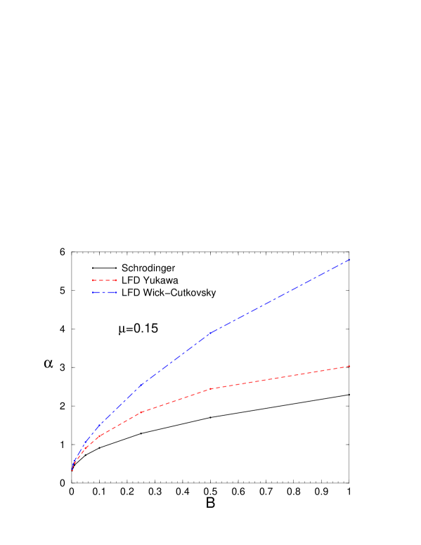
Figure 6: Comparison of $B(\alpha)$ between the Yukawa (dashed line) and Wick-Cutkosky (dot dashed lines) models in LFD and non relativistic (solid line) results in $J=0^{+}$ state

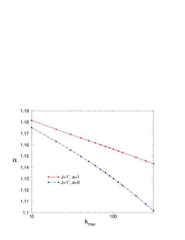
Figure 7: Logarithmic dependence of the coupling constant as a function of cutoff for the $J=1^{+}$ a=0 and a=1 states. Calculations correspond to B=0.05 and $\mu=0.25$

The system of equations for determining the $J=1^{+},a=0$ ($g^{(a=0)}_{i=1,2}$) and $a=1$ ($g^{(a=1)}_{i=1,2,3,4}$) solutions are both unstable and require cutoff regularization GHPSW_PRD47_93 ; MCK_PRD_01 . This can be seen in Fig. 7 where the $\alpha(k_{max})$ variation for $a=0$ and $a=1$ cases displays a logarithmic dependence. One can also see in this figure the non degeneracy of both states due to the Fock space truncation discussed in section III. We remark however that if the binding energies – or equivalently coupling constants – of states with different projections $a$ are not equal, they are almost-degenerated in a wide range of $k_{max}$ values. For instance, at $k_{max}=10$ one has $\alpha_{a=0}$=1.17 and $\alpha_{a=1}$=1.18 while at $k_{max}=90$ one has $\alpha_{a=0}$=1.14 and $\alpha_{a=1}$=1.16. These weak splitting – of less than 1% – for a noticeably bound system ($B=0.05$), are rather surprising in view of the results obtained in the purely scalar WC case MCK_Heid_00 ; KCM_Taiw_01 , in which the difference in coupling constants for the same binding energy is rather 20%, what corresponds to $\Delta B\approx B$.

The $g^{(a)}_{i}$ solutions for a=0 and a=1 states are respectively represented in Figs. 8 and 9 for several values of $\theta$. They were obtained with a coupling constant $\alpha_{s}=1.18$ and a sharp cutoff at $k_{max}=10$. We remark that with the conventions used $g^{(0)}_{2}(k,0)=0$ and on has $g^{(0)}_{1}(0,0)=-g^{(0)}_{2}(0,90^{\circ})$, as expected from (87). In addition: $g^{(0)}_{1}(0,0)=-g^{(0)}_{2}(0,90^{\circ})\approx g^{(1)}_{1}(0,\theta)$, as expected from (88) and from the fact that coefficient $c_{i}$, defined in (89), are very close to the values (90). Corresponding binding energies are $B_{a=0}=0.0506$ and $B_{a=1}=0.0498$, values which are 1% close to each other. The splitting of the binding energies is an increasing function of the coupling constant. Figure 10 shows the calculated $B_{a}(\alpha)$ dependence for both J=1 eigenstates. For $\alpha_{s}=0.55$ the values are respectively $B_{a=0}=9.7\,10^{-3}$ and $B_{a=1}=9.6\,10^{-3}$ whereas for $\alpha_{s}=2.87$ $B_{a=0}=0.523$ and $B_{a=1}=0.467$. The non degeneracy remains reasonably small even for strongly bound systems.

     

Figure 8: $g^{a=0}_{i=1,2}$ solutions for scalar coupling with $\alpha=1.18$, $\mu=0.25$ and sharp cutoff at $k_{max}=10$. Binding energy is $B=0.0506$.

Figure 9: $g^{a=1}_{i=1,\ldots,4}$ solutions for scalar coupling with $\alpha=1.18$, $\mu=0.25$ and sharp cutoff at $k_{max}=10$. Corresponding binding energy is $B=0.0498$

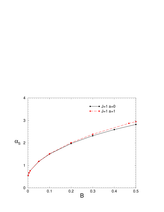
Figure 10: Splitting of the J=1 solutions for the scalar coupling. Results correspond to $\mu=0.25$ and sharp cut-off at kmax=10

The six components $f_{i}$ of the $J=1^{+}$ physical wave function are determined by a linear combination (83) of functions $f_{i}^{(a)}$ which in their turn are expressed in terms of $g_{i}^{(a)}$ by (55) and (73). We remind that coefficients $c_{a}$ of this linear combination are computed from components $g_{1}^{(a=0,1)}$ only. For the solutions presented in Figs. 8 and 9 they are found to be $c_{0}=0.582$ and $c_{1}=0.813$ and the corresponding energy is B=0.0501. Note that these values are very close to those obtained in case of $\vec{n}$-independent interactions (90): $c_{0}={1\over\sqrt{3}}=0.577$ and $c_{1}=\sqrt{\frac{2}{3}}=0.816$. They become even closer to these values for smaller binding energies and they smoothly depart for strongly bound systems. For a state with $B\approx 0.5$ and the same sharp cutoff $k_{max}=10$ one has for instance $c_{0}=0.610$ and $c_{0}=0.793$. Components $f_{i}$ thus obtained are displayed in Fig. 11 for $\theta=30$ degrees in linear (a) and logarithmic (b) scales. One can see that component $f_{1}$ dominates over all remaining five in all the momentum range. Among the components of relativistic origin there is not a clear dominance. Notice the very small value of $f_{2}$ component, corresponding to the tensor D-wave, that would be absent in a non relativistic approach. These components have a definite parity in variable $\cos\theta$, $f_{1,2,3,5}$ being even and $f_{4,6}$ odd, as shown in Fig. 11b for a fixed value $k=1$.

     

Figure 11: Wave function components $f_{i}$ of the physical solutions (a) as a function of $k$ at $\theta=30^{o}$ and (b) their $\theta$-dependence at fixed $k=1$ value. Calculations are for the scalar coupling with $\alpha=1.18$, $\mu=0.25$ and sharp cut-off $k_{max}=10$. Binding energy is B=0.0501.

VIII Results for pseudoscalar coupling

For pseudoscalar coupling, the stability analysis was performed using the same methods than for the scalar one MMB_These_01 ; MCK_LCM_01 and presents some peculiarities.

Equations for J=$0^{+}$ states are found to be stable without any regularization. The asymptotic behavior of the pseudoscalar kernel is the same than the scalar one it has a repulsive character which do not generates instability. The results lead to a quasidegeneracy of the coupling constants for binding energies which vary over all the physical range $[0,2m]$. One gets for instance, $\alpha=55.4$ for $B=0.001$ whereas $\alpha=58.5$ for a binding energy 500 times bigger $B=0.5$, showing an extreme sensibility of this model to small variations of the coupling constant. The origin of this behavior was found to lie in the second channel equation ($\kappa_{22}$) and has been understood analytically MCK_LCM_01 with a simple model. The use of form factors – though not required for the convergence of solutions – is necessary if one wishes to eliminate this unusual $\alpha(B)$ dependence. Calculations have thus been performed using form factors (19) with n=1 and $\Lambda$=1.3 as in the Bonn model.

In the weak binding limit (B=0.001) one has $\alpha_{LFD}=190$ and $\alpha_{NR}=166$, a repulsive effect much stronger (15%) than in the scalar coupling. Corresponding wave functions are shown in Fig. 12. One can see that the component of relativistic origin $f_{2}\approx f_{1}$ at $k\sim 0.3$ and dominates above $k$=1. A similar result was found in the np ${}^{1}S_{0}$ scattering wave function calculated perturbatively with all the OBEP kernel in CK_NPA589_95 . Contrary to the Yukawa model, the role of relativistic components is crucial already for such a loosely bound system. The coupling between components is also very important: by switching off the non diagonal kernels $K_{12}=K_{21}=0$ the coupling constant moves from $\alpha_{LFD}=190$ to $\alpha_{LFD}=251$. It has thus an attractive effect which tends to minimize the difference between LFD and NR results. The comparison between $f_{1}$ and the non relativistic solution $f_{NR}$ shows a very good agreement in the small $k$. When $k$ increases, large differences appear and $f_{NR}$ has even an additional zero at $k=1.1$.

Figure 12: Wave function components (in logarithmic scale) for $J=0^{+}$ state with B=0.001, $\mu=0.15$ obtained with pseudoscalar coupling and form factor $\Lambda=1.3$.

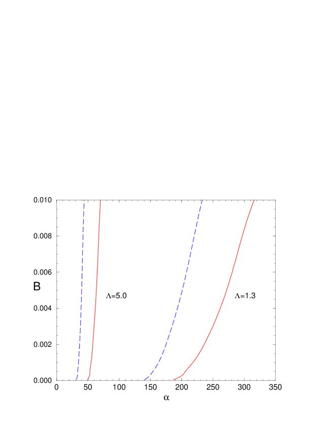
Figure 13: B($\alpha$) for pseudoscalar coupling and $J^{\pi}=0^{+}$ state with $\mu=0.5$ and two different form factors compared to non relativistic results

It is worth noticing the dramatic influence of the form factor in all these calculations. One has for instance $\alpha_{LFD}$=103 for $\Lambda=5$ and $\alpha_{LFD}$=1725 for $\Lambda$=0.3. We remind that the value used in the Bonn model for this coupling is $\Lambda_{Bonn}=1.3$.

Quite surprisingly, in the strong binding limit (B=0.5) we have found $\alpha_{LFD}$=1462 and $\alpha_{NR}$=3065. Relativistic effects become now strongly attractive ($\alpha_{LFD}<\alpha_{NR}$). An essential part of this attraction is due to the coupling of the two $f_{1}-f_{2}$ components in the LFD wave function. By performing one channel calculations, one has indeed $\alpha_{LFD}$=3001, what represents a strong reduction in the effect though it remains slightly attractive. We have checked if this attractive effect happens for different values of the exchange mass $\mu$. For the same binding energy ($B=0.5$) and $\mu=0.5$ we have found $\alpha_{LFD}$=1728 and $\alpha_{NR}$=1400, repulsive once again. It is worth noticing that for this coupling $\alpha_{NR}$ is a decreasing function of $\mu$ whereas $\alpha_{LFD}$ increases, at least in this energy region. This tells us the difficulty of talking about the ”sign of relativistic effects” in general. They turn to depend not only on the kind of coupling but also on the binding energy of the system and - furthermore - on the mass of the exchanged particle.

It is interesting to study the zero binding limit of the LFD results and compare them with the non relativistic ones. The NR potential (94) has been modified by including the Bonn form factor (19). The results are given in Fig. 13 for an exchange mass $\mu=0.5$ and with two different cutoff parameters $\Lambda$ in the form factors. They show the same behavior that was found in the scalar case MC_PLB_00 i.e. that the relativistic and non relativistic approaches do not coincide even when describing systems with zero binding energies as far as they interact with massive exchanges.

The $J=1$ state displays the same kind of departures from the scalar case than $J=0$. Functions $g^{(a)}_{i}$ for $a=0,1$ have been calculated using the values $\alpha_{PS}=60$, $\mu=0.25$ and $\Lambda=1.3$. Contrary to the scalar case, binding energies are sizeably different: $B_{a=0}=0.103$ whereas $B_{a=1}=0.0494$. The physical wave function is obtained using the same procedure than for the scalar case, i.e. compute $f^{a=0,1}_{i=1,6}$ and extract from them the coefficients $c_{i}$. Their values, $c_{0}=0.749$ and $c_{1}=0.662$, are different from $c_{0}\approx{1\over\sqrt{3}},c_{1}\approx\sqrt{2\over 3}$ with $c_{0}$ bigger than $c_{1}$. The averaged binding energy is $B=0.0793$. The corresponding solutions are plotted in Figs. 14. One can see that $f_{1}$ dominates at small momenta ($k<<1$) but starting from $k\sim 1$, the components of relativistic origin become larger than $f_{1}$.

Figure 14: Physical solutions for $J=1^{+}$ state with PS coupling. Parameters are $\alpha=60$, $\mu=0.25$, $\Lambda=1.3$. Corresponding binding energy is $B=0.079$ and components are plotted for $\theta=30^{o}$.

The splitting in binding energies is much bigger than for the scalar coupling. It can be seen in Figure 15a where the results of $B_{a}(\alpha)$ for both $\hat{A}^{2}$ eigenstates are plotted. The energy differences remain important even in the $B\to 0$ limit – Figure 15b – in accordance with the analytical considerations in section VI.

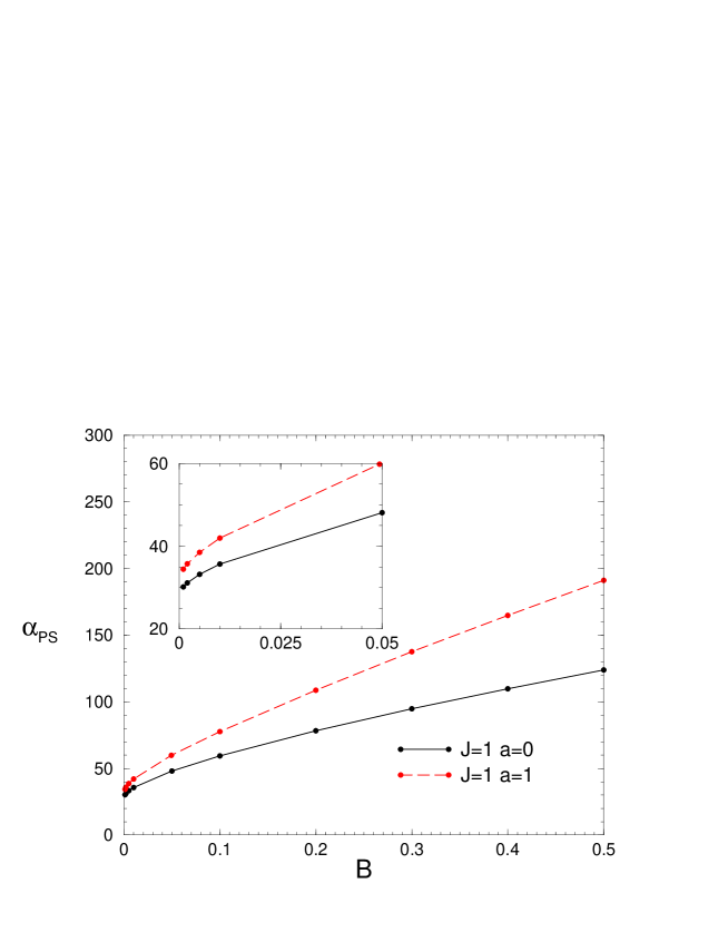
Figure 15: Splitting of the J=1 solutions for pseudoscalar coupling. Results correspond to $\mu=0.25$ and $\Lambda$=1.3, $n$=1

In summary, as it was noticed in Section VI, pseudoscalar coupling displays the largest deviations with respect to the non relativistic dynamics. Small and large spinor components are mixed to the first order. The coupling between $f_{1}$ and $f_{2}$ is essential even for very weakly bound systems, the components of relativistic origin dominates already at moderates values of $k$ and the splitting of the binding energies for the different projections of the $J\neq 0$ states are of the same order than the energies themselves.

IX Results for vector coupling

The stability analysis applied to vector kernels shows that vertex form factors are required for both $J=0^{+}$ and $J=1^{+}$ states to obtain stable solutions.

This is true in particular in the simplest application of vector coupling: the positronium $J=0^{-}$ state. The negative parity of the state comes from the intrinsic positron parity so that the corresponding kernels are those of the $J^{\pi}=0^{+}$ two-fermion system already given in Appendix A. In Table 1 are presented the values of the coupling constant $\alpha$ as a function of the sharp cut-off $k_{max}$ and for a fixed binding energy $B=0.0225$. The dependence is very slow – 0.3% variation for $k_{max}\in[10,300]$ – but it actually corresponds to a logarithmic divergence of $\alpha(k_{max})$ as it can be seen in Fig. 16. The origin of this instability is the coupling to the second component, whose kernel matrix element $\kappa_{22}$ has an attractive, constant asymptotic limit. If one removes this component – which has a very small contribution in norm – calculations become stable and give for $\alpha_{NR}=0.30$ the value $\alpha_{LFD}=0.3975$.

Table 1: Coupling constant $\alpha$ as a function of the sharp cut-off $k_{max}$ for the $J=0^{-}$ positronium state with binding energy $B=0.0225$ a.u.

$k_{max}$	10	20	30	40	50	70	100	200	300
$\alpha$	0.3945	0.3928	0.3918	0.3911	0.3905	0.3896	0.3887	0.3867	0.3854

The comparison of LFD ladder results with those obtained in perturbative QED or to the physical energies is meaningless due to the instability of the solutions themselves. The use of vertex form factors in a system of pointlike particles would be hazardous and the introduction of renormalizable counterterms seems to be a more appropriate cure.

First positronium results in Light Front Dynamics were obtained in GPW_PRD45_92 ; TP_NP90_00 . These authors introduced a large number of states in the Fock expansion but observed the same instability of the solutions. For a fixed value of the cut-off, the results become finite and can be compared. By taking $k_{max}=10$ and $\alpha=0.3$ – which corresponds to $B_{NR}=0.0225$ – we found $B_{LFD}=0.0132$, i.e. repulsive relativistic effects. The leading order QED corrections BS_QM_77 reads

$$B_{QED}={\alpha^{2}\over 4}\left[1+\frac{21}{16}\alpha^{2}+o(\alpha^{4})\right]\approx 0.02516,$$

and are so attractive. Equation (10) from TP_NP90_00 gives for $k_{max}=10$ the value $B_{DLC}=0.0308$, in qualitative agreement – thought still sizeably different – with $B_{QED}$. We should notice that a recent work Tritmann_IJMP_01 analyzes the results of TP_NP90_00 in terms of flow equations and obtains a closer value $B_{DLC}=0.02341$. We conclude from that, that the ladder LFD predictions for such a genuine system are unable to reproduce even the sign of first order relativistic corrections. Because the lowest order corrections of the singlet state are not affected by the annihilation channels, the differences could be due to cross ladder graphes.

Figure 16: Coupling constant $\alpha$ as a function of the sharp cut-off $k_{max}$ for the $J=0^{-}$ positronium state with binding energy $B=0.0225$ a.u.

For $\mu\neq 0$, the two fermion system is bound due to the $\mu$-dependent terms ($\sim{tt^{\prime}\over\mu^{2}}\upsilon_{ij}$) in the vector kernel (121), since the $\mu$-independent ones ($\chi_{ij}$) are repulsive. This binding disappear in the non relativistic limit.

When solving the equations for $J=0^{+}$ state, the standard form factors (19) – depending on $Q^{2}$ and local in the non relativistic limit – were found to be insufficient for any power $n$ to ensure stable solution. A $Q^{2}$ dependent gaussian form factor failed as well. This unstability comes from the $\mu$-dependent terms. These are off-shell corrections depending on variables $t,t^{\prime}$ defined by

$$4m^{2}t=4\varepsilon^{2}_{k}-M^{2},\qquad 4m^{2}t^{\prime}=4\varepsilon^{2}_{k^{\prime}}-M^{2}$$ (110)

and are not regularized by a form factor depending on variable $Q^{2}$. Such a function cuts off the high $|\vec{k}-\vec{k^{\prime}}|$ components, but not the $|\vec{k}+\vec{k^{\prime}}|$ ones. A similar situation is encountered in the framework of chiral perturbation theory EGM_NPA67_00 and was solved by the replacement $\kappa(k,k^{\prime})\to F(k)\kappa(k,k^{\prime})F(k^{\prime})$.

Our way of doing is the following. Variable $Q^{2}=-(k_{meson}-\omega\tau_{1})^{2}$ entering $F(Q^{2})$ is associated with the off-energy shell effects in the intermediate state containing one massive meson ($\mu$). In a similar way, we introduce the variable $\eta=m^{2}-(k_{1}-\omega\tau)^{2}$ – see vertex 2 in the first graph of Fig. 3 – and correspondingly $\eta^{\prime}=m^{2}-(k^{\prime}_{2}-\omega\tau^{\prime})^{2}$ from vertex 1. Variables $\eta,\eta^{\prime}$ control the off-energy shell contribution to the fermion states and have been regularized by means of a cut-off function

$$H(\eta)=\left(\Lambda^{2}\over\Lambda^{2}+\eta\right)^{n}.$$

This corresponds to a non-local form factor even in the non relativistic limit. On energy shell one has $\eta=\eta^{\prime}=0$.

Thus, for instance, the total form factor associated with vertex 2 in of Fig. 3 reads:

$$F_{nloc}(Q^{2},\eta)=F(Q^{2})H(\eta)$$ (111)

In center of mass variables (3) the expressions for $\eta,\eta^{\prime}$ are:

$$\eta=\left\{\begin{array}[]{ll}(1-{\vec{k}\makebox[2.27626pt]{$\cdot$}\vec{n}\over\varepsilon_{k}})\;2m^{2}t&\rm{if\;\;{\vec{k}\,^{\prime}\makebox[2.27626pt]{$\cdot$}\vec{n}\over\varepsilon_{k^{\prime}}}-{\vec{k}\cdot\vec{n}\over\varepsilon_{k}}>0}\\ (1+{\vec{k}\makebox[2.27626pt]{$\cdot$}\vec{n}\over\varepsilon_{k}})\;2m^{2}t&\rm{if\;\;{\vec{k}\,^{\prime}\makebox[2.27626pt]{$\cdot$}\vec{n}\over\varepsilon_{k^{\prime}}}-{\vec{k}\makebox[2.27626pt]{$\cdot$}\vec{n}\over\varepsilon_{k}}<0}\end{array}\right.$$ (112)

and

$$\eta^{\prime}=\left\{\begin{array}[]{ll}(1+{\vec{k}\,^{\prime}\makebox[2.27626pt]{$\cdot$}\vec{n}\over\varepsilon_{k^{\prime}}})\;2m^{2}t^{\prime}&\rm{if\;\;{\vec{k}\,^{\prime}\cdot\vec{n}\over\varepsilon_{k^{\prime}}}-{\vec{k}\makebox[2.27626pt]{$\cdot$}\vec{n}\over\varepsilon_{k}}>0}\\ (1-{\vec{k}\,^{\prime}\makebox[2.27626pt]{$\cdot$}\vec{n}\over\varepsilon_{k^{\prime}}})\;2m^{2}t^{\prime}&\rm{if\;\;{\vec{k}\,^{\prime}\makebox[2.27626pt]{$\cdot$}\vec{n}\over\varepsilon_{k^{\prime}}}-{\vec{k}\makebox[2.27626pt]{$\cdot$}\vec{n}\over\varepsilon_{k}}<0}\end{array}\right.$$ (113)

with $t,t^{\prime}$ given defined in (110).

Each coupling constant is replaced by $g\to gF(Q^{2})H(\eta)$ – or $g\to gF(Q^{2})H(\eta^{\prime})$ – and the kernel is multiplied by $F^{2}(Q^{2})H(\eta)H(\eta^{\prime})$. The values for $\Lambda$ and $n$ in $H$ are taken the same than for $F(Q^{2})$, but could in principle be different.

     

Figure 17: Wave functions $f_{i}$ for a $J^{\pi}=0^{+}$ state in the vector coupling with $\mu=0.15$ and using the non-local form factor (111) with n=1 and $\Lambda=1.3$. The coupling constant is $\alpha=1.485$ and the binding energy $B=0.0225$.

By means of (111), the solutions become stable but we notice that the use of only one kind of form factor is not enough to ensure the stability. Wave functions corresponding to $\mu=0.15$ obtained with $n=1$ and $\Lambda=1.3$ in (111) are displayed in Fig. 17. Binding energy is B=0.0225 and $\alpha_{v}=1.485$. They have normal behavior and one remarks sizeable relativistic component $f_{2}$ starting from $k\approx 0.5$ with a strong $\theta$-dependence despite the small binding energy of the state.

Let us now consider the $J^{\pi}=1^{+}$ state. Solving the $J^{\pi}=1^{+},a=0$ equations with the $F(Q^{2})$ form factor only, leads to the same anomalies than for $J^{\pi}=0^{+}$. With the non-local form factor the situations is regularised. With parameters $B=0.050$, $\mu=0.25$, $\Lambda=1.3$ and $n=1$ for instance, one has a coupling constant $\alpha=6.18$ and a well behaved wave function. The same happens for the $J^{\pi}=1^{+},a=1$ state. When using, with the same parameters, the non-local form factor (111), we get $\alpha=6.01$.

The mass splitting between the two $a=0,1$ projections is shown in Fig. 18. One first remark the striking behavior of $\alpha_{a}(B)$ curves, i.e. larger binding energies correspond to smaller values of the coupling constant $\alpha$. This fact – which takes place also for $J=0^{+}$ states – is a consequence of the $M^{2}$-dependence of the $\frac{tt^{\prime}}{\mu^{2}}$ terms driving the vector kernel $\kappa_{ij}^{(\mu)}$ in (121). Its contribution is large, because of $\mu^{2}$ in denominator. Increasing the binding energy – i.e. decreasing $M^{2}$ – increases $t,t^{\prime}$ factors, and results into smaller values of $\alpha$. When the $M^{2}$ dependence in $t,t^{\prime}$ kernel is frozen – setting e.g. $M^{2}=4m^{2}$ – the usual $\alpha(B)$ variation is recovered (dotted curve in Figure 18). When including the full dynamics, both $\alpha_{a}(B)$ curves get close each other in all the variation domain $B=[0,0.5]$, as it was the case in the scalar coupling. However due to their peculiar behavior – flat and almost parallel – the splitting in binding energies corresponding to a fixed value of the coupling constant, can be very large. One can also remark in Fig. 18 the different values of $\alpha_{a}$ at B=0 despite the fact that the systems of equations for a=0 and a=1 have – as in the scalar coupling – the same non-relativistic limit. This difference is due to the $1/\mu^{2}$ terms in the kernel. They are not relevant at the $(1/m)^{0}$ order but are crucial for binding a relativistic two-fermion system by vector exchange. For a fermion-antifermion system with massless exchange, e.g. positronium, the splitting at B=0 disappears.

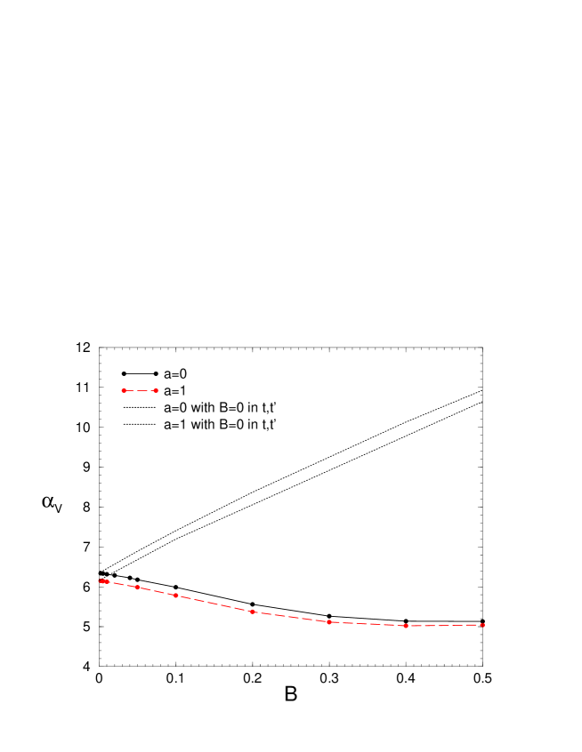
Figure 18: Splitting of the $J=1^{+}$ solutions for vector coupling with $\mu=0.25$ and form factors (111) with $\Lambda=1.3$ n=1. Dotted lines correspond to a fixed binding energy (B=0) in $t,t^{\prime}$ off-shell variables of kernel (121)

X Conclusion

We have presented the explicitly covariant LFD solutions for the bound state of two fermion systems in the ladder approximation. A method for constructing non zero angular momentum states has been proposed and illustrated by numerical examples. It is based on satisfying the angular condition by a linear superposition of eigenstates of an operator commuting with the LFD ladder hamiltonian.

We have separately examined the different types of OBE couplings and found very different behaviours concerning the stability of the solutions themselves and their relation with the corresponding non relativistic reductions.

Scalar coupling (Yukawa model) is found to be stable without any kernel regularization for the $J^{\pi}=0^{+}$ state and coupling constants below some critical value $\alpha<\alpha_{c}=3.72$. For values above $\alpha_{c}$ the system collapses. For $J^{\pi}=1^{+}$ state the solutions of both a=0 and a=1 projections are unstable. Their energy splitting is very small even for binding energies (B) of the same order than the constituents mass and vanishes at B=0. The physical solution, satisfying the angular condition, has been constructed by a suitable linear combination of a=0,1 states. LFD binding energies are found to be close to those given by their non relativistic limit, even closer than the case of purely scalar particles (Wick Cutkosky model extended to $\mu\neq 0$). The comparison with the non relativistic solutions shows always repulsive effects. The LFD wavefunction is dominated by the components which has non-relativistic counterpart. Extra components of relativistic origin remain negligible even at large values of the relative momentum ($k>m$).

Pseudoscalar coupling is also found stable for $J^{\pi}=0^{+}$ state. It displays a very strong dependence of binding energies as a function of the coupling constant: they vary from B=0.001 to B=0.500 (in constituent mass units) while the coupling constant changes from $\alpha=55.5$ to $\alpha=58.5$. This dependence is due to the coupling to the wave function component of relativistic origin. Vertex form factors are required for $J^{\pi}=1^{+}$ states. LFD solutions, obtained with regularized kernels, presents large deviations with respect to non relativistic case, even for weakly bound states, and display a big sensitivity to the cut-off parameters. The LFD wave function is dominated by relativistic component at relatively small momenta ($k<m$). The coupling between different components is strongly attractive and can compensate the repulsive effects observed in the Yukawa model. Thus, relativistic corrections can be attractive or repulsive depending on the quantum number of state, the value of the binding energy and even the mass $\mu$ of the exchanged meson. The energy splitting between different projections of $J=1$ states is large and remains at B=0.

Vector coupling presents the stronger anomalies. For $\mu=0$ it has been applied to positronium $0^{+}$ state. It is found to be unstable and, once regularized by means of sharp cut-off, the ladder approximation gives relativistic corrections of opposite sign compared to QED perturbative results. This failure shows the poorness of the ladder approximation in one of the rare cases in which it can be confronted to experimental results. For $\mu\neq 0$ the LFD solutions collapse even using local cutoff form factors. The reason lies in the strong non-localities of the $\mu$-dependent terms in the LFD kernel. These terms have their origin in the massive vector propagator and manifest as off-shell corrections of the $\mu=0$ kernels. They have been regularized using appropriate vertex form factors. The $J=1^{+}$ state has thus been calculated. This state is not bound in the non relativistic limit and its existence in a relativistic approach is entirely due to the $\mu$-dependent terms in the kernel The importance of this off-shell terms is thus dramatic. In particular their energy dependence generates a decreases of the binding energy as a function of the coupling constant, what questions the very meaning of the interaction strength. The $\alpha_{a}(B)$ dependence for different projections of $J=1$ states remain very close to each other even for $B\sim m$ but their particular form – smooth and almost parallel variation – can give rise to large energy splitting for a fixed value of the coupling constant.

Some general additional remarks concerning the relativistic calculations are given in order.

• Contrary to the non relativistic case, vertex form factors are unavoidable in any realistic calculation. The full spinor structure generates highly singular kernels which are not regularized by local vertex form factors. It is clear that specially at large k-values, the obtained wave function and consequently the electromagnetic form factors will crucially depend on the way the regularization is performed. The large momentum components will thus be determined not by the dynamics but by uncontrolled parameters. We believe that here is the main drawback of relativistic approaches.

• The consequences of implementing the Lorentz invariance in a quantum mechanical description of a system are not only kinematical but mainly dynamical. Large differences with respect to the non relativistic solutions appear even in the zero binding limit for systems with ${k\over m}\ll 1$ as far as the exchanged mass is non zero. We have explicitly shown for scalar and pseudoscalar couplings that the behavior of $\alpha(B)$ at $B\approx 0$ differs from their non relativistic counterparts, a result already found in the Wick-Cutkosky model MC_PLB_00 .

• The question about the sign of relativistic effects has no simple answer. They can be different, following: the nature of the constituents, the kind of interaction, the quantum numbers of the state, its binding energy, and even the mass of the exchanged particle. This shows that there are no simple recipes to perform a priori evaluations.

• The splitting of different projections of J=1 states is very different following the kind of coupling. In nuclear physics – where the weight of scalar mesons in the binding energy is dominating – is expected to be very small. The same is true for the massless vector coupling like one-photon or one-gluon exchange. It can be however very large in relativistic models where pseudoscalar exchange plays an important role.

Finally we would to emphasize one of the interest of using LFD in describing the relativistic composite systems. It lies in the fact that wave functions components appearing in this approach are closely related to their non relativistic counterparts. Some of these components are the formal equivalent of the usual non relativistic solutions while others are of pure relativistic origin. Relativity manifests both in modifying the former and in giving a sizeable weight to the latter ones. We have found that the coupling between these components plays an essential role, even in determining the stability of the solutions. In addition – except for the scalar exchange – the total wave function is dominated by the relativistic components at moderate values of its arguments ($k<m$) and that, even for loosely bound systems.

Acknowledgements. One of the authors (V.A.K.) is sincerely grateful for the warm hospitality of the theory group at the Institut des Sciences Nucléaires de Grenoble, where this work was performed. Numerical calculations were carried out at CGCV (CEA Grenoble) and IDRIS (CNRS). We thank the staff members of these organizations for their constant support. This work is partially supported by the French-Russian PICS and RFBR grants Nos. 1172 and 01-02-22002 as well as by the RFBR grant 02-02-16809.

Appendix A Kernels

Kernels $\kappa_{ij}$ are obtained from equations (47), (48), (70) and (71) as traces of 4x4 matrices. To calculate these traces, it is useful to express the scalar products between all the concerned four-vectors in terms of variables $(k,k^{\prime},\theta,\theta^{\prime})$. They read:

$$\omega^{2} = 0,$$

$$k_{1}^{2} = k_{2}^{2}=k^{\prime 2}_{1}=k^{\prime 2}_{2}=m^{2},$$

$$\omega\makebox[2.27626pt]{$\cdot$}k_{1} = x\,\omega\makebox[2.27626pt]{$\cdot$}p,$$

$$\omega\makebox[2.27626pt]{$\cdot$}k_{2} = (1-x)\,\omega\makebox[2.27626pt]{$\cdot$}p,$$

$$\omega\makebox[2.27626pt]{$\cdot$}k^{\prime}_{1} = x^{\prime}\,\omega\makebox[2.27626pt]{$\cdot$}p,$$

$$\omega\makebox[2.27626pt]{$\cdot$}k^{\prime}_{2} = (1-x^{\prime})\,\omega\makebox[2.27626pt]{$\cdot$}p,$$

$$k_{1}\makebox[2.27626pt]{$\cdot$}k_{2} = 2\varepsilon_{k}^{2}-m^{2},$$

$$k^{\prime}_{1}\makebox[2.27626pt]{$\cdot$}k^{\prime}_{2} = 2\varepsilon_{k^{\prime}}^{2}-m^{2},$$

$$k_{1}\makebox[2.27626pt]{$\cdot$}p = 2\varepsilon_{k}^{2}(1-x)+\frac{1}{2}M^{2}x,$$

$$k_{2}\makebox[2.27626pt]{$\cdot$}p = 2\varepsilon_{k}^{2}x+\frac{1}{2}M^{2}(1-x),$$

$$k^{\prime}_{1}\makebox[2.27626pt]{$\cdot$}p = 2\varepsilon_{k^{\prime}}^{2}(1-x^{\prime})+\frac{1}{2}M^{2}x^{\prime},$$

$$k^{\prime}_{2}\makebox[2.27626pt]{$\cdot$}p = 2\varepsilon_{k^{\prime}}^{2}x+\frac{1}{2}M^{2}(1-x^{\prime}),$$

$$k_{1}\makebox[2.27626pt]{$\cdot$}k^{\prime}_{1} = -kk^{\prime}\sin\theta\sin\theta^{\prime}\cos\phi+2\varepsilon_{k^{\prime}}^{2}x+2\varepsilon_{k}^{2}x^{\prime}-2\varepsilon_{k}^{2}xx^{\prime}-2\varepsilon_{k^{\prime}}^{2}xx^{\prime},$$

$$k_{2}\makebox[2.27626pt]{$\cdot$}k^{\prime}_{2} = -kk^{\prime}\sin\theta\sin\theta^{\prime}\cos\phi+2\varepsilon_{k}^{2}x+2\varepsilon_{k^{\prime}}^{2}x^{\prime}-2\varepsilon_{k}^{2}xx^{\prime}-2\varepsilon_{k^{\prime}}^{2}xx^{\prime},$$

$$k_{1}\makebox[2.27626pt]{$\cdot$}k^{\prime}_{2} = kk^{\prime}\sin\theta\sin\theta^{\prime}\cos\phi+2\varepsilon_{k}^{2}(1-x)(1-x^{\prime})+2\varepsilon_{k^{\prime}}^{2}xx^{\prime},$$

$$k_{2}\makebox[2.27626pt]{$\cdot$}k^{\prime}_{1} = kk^{\prime}\sin\theta\sin\theta^{\prime}\cos\phi+2\varepsilon_{k^{\prime}}^{2}(1-x)(1-x^{\prime})+2\varepsilon_{k}^{2}xx^{\prime},$$ (114)

where

$$x=\frac{1}{2}(1-\frac{k}{\varepsilon_{k}}\cos\theta)\qquad x^{\prime}=\frac{1}{2}(1-\frac{k^{\prime}}{\varepsilon_{k^{\prime}}}\cos\theta^{\prime})$$ (115)

Using the above result, we have obtained the analytical expressions of $\kappa_{ij}$ kernels for $J^{\pi}=0^{+},1^{+}$ states. They are written below, coupling by coupling, in the form

$$\kappa_{ij}(k,\theta,k^{\prime},\theta^{\prime},\varphi^{\prime})=c_{ij}(k,\theta,k^{\prime},\theta^{\prime})+d_{ij}(k,\theta,k^{\prime},\theta^{\prime})\cos\varphi^{\prime}+e_{ij}(k,\theta,k^{\prime},\theta^{\prime})\cos^{2}\varphi^{\prime}$$ (116)

with coefficients $c_{ij},d_{ij},e_{ij}$ invariant under the transformation $(i,k,\theta)\leftrightarrow(i^{\prime},k^{\prime},\theta^{\prime})$. We introduce for shortness the notations

$$s\theta=\sin\theta\quad c\theta=\cos\theta\quad S\theta=k\sin\theta\quad C\theta=k\cos\theta\quad c\varphi^{\prime}=\cos\varphi^{\prime}$$

– plus corresponding primed – and the following quantities

$$b_{\pm}^{2} = m^{2}(\varepsilon_{k}^{2}+\varepsilon_{k^{\prime}}^{2})\pm 2\varepsilon_{k}^{2}\varepsilon_{k^{\prime}}^{2}$$

$$\varepsilon_{k}^{\pm} = \varepsilon_{k}\pm m$$

$$\Delta^{\pm} = \varepsilon_{k}^{2}\pm\varepsilon_{k^{\prime}}^{2}$$

Coupling constants appear through $\alpha={g^{2}\over 4\pi}$.

A.1 Scalar

Kernels for the scalar coupling were already given in MCK_PRD_01 and are included here for completeness.

$J=0^{+}$:

$${\kappa_{11}\over\alpha\pi} = -[m^{2}\Delta^{+}+2\varepsilon_{k}\varepsilon_{k^{\prime}}(\varepsilon_{k}\varepsilon_{k^{\prime}}-C\theta C\theta^{\prime})]+\Delta^{+}S\theta S\theta^{\prime}c\varphi^{\prime}$$

$${\kappa_{12}\over\alpha\pi} = -m\Delta^{-}(S\theta^{\prime}+S\theta c\varphi^{\prime})$$

$${\kappa_{21}\over\alpha\pi} = +m\Delta^{-}(S\theta+S\theta^{\prime}c\varphi^{\prime})$$ (117)

$${\kappa_{22}\over\alpha\pi} = \Delta^{+}S\theta S\theta^{\prime}-[m^{2}\Delta^{+}+2\varepsilon_{k}\varepsilon_{k^{\prime}}(\varepsilon_{k}\varepsilon_{k^{\prime}}-C\theta C\theta^{\prime})]c\varphi^{\prime}$$

$J=1^{+},a=0$:

$${\kappa_{11}\over\alpha\pi} = [2kk^{\prime}\varepsilon_{k}\varepsilon_{k^{\prime}}-b_{+}^{2}c\theta c\theta^{\prime}]-\varepsilon_{k}\varepsilon_{k^{\prime}}\Delta^{+}s\theta s\theta^{\prime}c\varphi^{\prime}$$ (118)

$${\kappa_{12}\over\alpha\pi} = m\varepsilon_{k^{\prime}}(2\varepsilon_{k}^{2}+\Delta^{+})c\theta s\theta^{\prime}-m\varepsilon_{k}(2\varepsilon_{k^{\prime}}^{2}+\Delta^{+})s\theta c\theta^{\prime}c\varphi^{\prime}$$

$${\kappa_{21}\over\alpha\pi} = m\varepsilon_{k}(2\varepsilon_{k^{\prime}}^{2}+\Delta^{+})s\theta c\theta^{\prime}-m\varepsilon_{k^{\prime}}(2\varepsilon_{k}^{2}+\Delta^{+})c\theta s\theta^{\prime}c\varphi^{\prime}$$

$${\kappa_{22}\over\alpha\pi} = -\varepsilon_{k}\varepsilon_{k^{\prime}}\Delta^{+}s\theta s\theta^{\prime}+\left[2kk^{\prime}\varepsilon_{k}\varepsilon_{k^{\prime}}-b_{+}^{2}c\theta c\theta^{\prime}\right]c\varphi^{\prime}$$

$J=1^{+},a=1$:

$${2\kappa_{11}\over\alpha\pi} = -\left\{m\varepsilon_{k}s^{2}\theta(\Delta^{+}+2\varepsilon_{k^{\prime}}^{2})+m\varepsilon_{k^{\prime}}s^{2}\theta^{\prime}(\Delta^{+}+2\varepsilon_{k}^{2})+(c^{2}\theta+c^{2}\theta^{\prime})b_{+}^{2}-4\varepsilon_{k}\varepsilon_{k^{\prime}}C\theta C\theta^{\prime}\right\}$$

$$- \left\{\Delta^{+}(\varepsilon_{k}^{-}\varepsilon_{k^{\prime}}^{-}c\theta c\theta^{\prime}-kk^{\prime})s\theta s\theta^{\prime}\right\}c\varphi^{\prime}-\left\{\Delta^{+}\varepsilon_{k}^{-}\varepsilon_{k^{\prime}}^{-}s^{2}\theta s^{2}\theta^{\prime}\right\}c^{2}\varphi^{\prime}$$

$${2\kappa_{12}\over\alpha\pi} = [m\varepsilon_{k}(\Delta^{+}+2\varepsilon_{k^{\prime}}^{2})-b_{+}^{2}]s^{2}\theta-[m\varepsilon_{k^{\prime}}(\Delta^{+}+2\varepsilon_{k}^{2})-b_{+}^{2}]s^{2}\theta^{\prime}$$

$$- \left\{kk^{\prime}(\varepsilon_{k}-\varepsilon_{k^{\prime}})^{2}+(\varepsilon_{k}+\varepsilon_{k^{\prime}})^{2}\varepsilon_{k}^{-}\varepsilon_{k^{\prime}}^{-}c\theta c\theta^{\prime}\right\}s\theta s\theta^{\prime}c\varphi^{\prime}+\left\{\varepsilon_{k^{\prime}}^{-}(\varepsilon_{k}+\varepsilon_{k^{\prime}})^{2}c^{2}\theta^{\prime}-\varepsilon_{k^{\prime}}^{+}(\varepsilon_{k}-\varepsilon_{k^{\prime}})^{2}\right\}\varepsilon_{k}^{-}s^{2}\theta c^{2}\varphi^{\prime}$$

$${\sqrt{2}\kappa_{13}\over\alpha\pi} = -2\varepsilon_{k}\varepsilon_{k^{\prime}}C\theta S\theta^{\prime}-\varepsilon_{k^{\prime}}^{-}(m\Delta^{+}-2\varepsilon^{2}_{k}\varepsilon_{k^{\prime}})c\theta^{\prime}s\theta^{\prime}$$

$$+ \left\{2\varepsilon_{k}\varepsilon_{k^{\prime}}kC\theta^{\prime}+\varepsilon_{k}^{-}c\theta\left[\varepsilon_{k^{\prime}}(\Delta^{+}-2m\varepsilon_{k})-\varepsilon_{k^{\prime}}^{-}(\varepsilon_{k}+\varepsilon_{k^{\prime}})^{2}c^{2}\theta^{\prime}\right]\right\}s\theta c\varphi^{\prime}-(\varepsilon_{k}+\varepsilon_{k^{\prime}})^{2}\varepsilon_{k}^{-}\varepsilon_{k^{\prime}}^{-}s^{2}\theta s\theta^{\prime}c\theta^{\prime}c^{2}\varphi^{\prime}$$

$${\sqrt{2}\kappa_{14}\over\alpha\pi} = \Delta^{-}\left\{(m+\varepsilon_{k}^{-}s^{2}\theta)S\theta^{\prime}+mS\theta c\varphi^{\prime}-\varepsilon_{k}^{-}s^{2}\theta S\theta^{\prime}c^{2}\varphi^{\prime}\right\}$$

$${2\kappa_{21}\over\alpha\pi} = [m\varepsilon_{k^{\prime}}(\Delta^{+}+2\varepsilon_{k}^{2})-b_{+}^{2}]s^{2}\theta^{\prime}-[m\varepsilon_{k}(\Delta^{+}+2\varepsilon_{k^{\prime}}^{2})-b_{+}^{2}]s^{2}\theta$$

$$- \left\{kk^{\prime}(\varepsilon_{k}-\varepsilon_{k^{\prime}})^{2}+(\varepsilon_{k}+\varepsilon_{k^{\prime}})^{2}\varepsilon_{k^{\prime}}^{-}\varepsilon_{k}^{-}c\theta c\theta^{\prime}\right\}s\theta s\theta^{\prime}c\varphi^{\prime}+\left\{\varepsilon_{k}^{-}(\varepsilon_{k^{\prime}}+\varepsilon_{k})^{2}c^{2}\theta-\varepsilon_{k}^{+}(\varepsilon_{k^{\prime}}-\varepsilon_{k})^{2}\right\}\varepsilon_{k^{\prime}}^{-}s^{2}\theta^{\prime}c^{2}\varphi^{\prime}$$

$${2\kappa_{22}\over\alpha\pi} = m(\varepsilon_{k}+\varepsilon_{k^{\prime}})^{3}-\varepsilon_{k}^{-}(m\Delta^{+}-2\varepsilon_{k}\varepsilon_{k^{\prime}}^{2})c^{2}\theta-\varepsilon_{k^{\prime}}^{-}(m\Delta^{+}-2\varepsilon_{k}^{2}\varepsilon_{k^{\prime}})c^{2}\theta^{\prime}-4\varepsilon_{k}\varepsilon_{k^{\prime}}C\theta C\theta^{\prime}$$

$$- (\varepsilon_{k}+\varepsilon_{k^{\prime}})^{2}(\varepsilon_{k}^{-}\varepsilon_{k^{\prime}}^{-}-C\theta C\theta^{\prime})s\theta s\theta^{\prime}c\varphi^{\prime}$$

$$- \left\{2b_{+}^{2}(c^{2}\theta+c^{2}\theta^{\prime})+2m[\varepsilon_{k}(\Delta^{+}+2\varepsilon_{k^{\prime}}^{2})s^{2}\theta+\varepsilon_{k^{\prime}}(\Delta^{+}+2\varepsilon_{k}^{2})s^{2}\theta^{\prime}]+(\varepsilon_{k}+\varepsilon_{k^{\prime}})^{2}\varepsilon_{k}^{-}\varepsilon_{k^{\prime}}^{-}s^{2}\theta s^{2}\theta^{\prime}-8\varepsilon_{k}\varepsilon_{k^{\prime}}C\theta C\theta^{\prime}\right\}c^{2}\varphi^{\prime}$$

$${\sqrt{2}\kappa_{23}\over\alpha\pi} = \left\{2k^{\prime}\varepsilon_{k}\varepsilon_{k^{\prime}}C\theta+\varepsilon_{k^{\prime}}^{-}(m\Delta^{+}-2\varepsilon^{2}_{k}\varepsilon_{k^{\prime}})c\theta^{\prime}\right\}s\theta^{\prime}-\left\{\varepsilon_{k}^{-}c\theta\left[\varepsilon_{k^{\prime}}^{-}(\varepsilon_{k}+\varepsilon_{k^{\prime}})^{2}c^{2}\theta^{\prime}-\varepsilon_{k^{\prime}}(\Delta^{+}-2m\varepsilon_{k})\right]-2k\varepsilon_{k}\varepsilon_{k^{\prime}}C\theta^{\prime}\right\}s\theta c\varphi^{\prime}$$

$$- \left\{\varepsilon_{k^{\prime}}^{-}c\theta^{\prime}\left((\varepsilon_{k}-\varepsilon_{k^{\prime}})^{2}\varepsilon_{k}^{+}-(\varepsilon_{k}+\varepsilon_{k^{\prime}})^{2}\varepsilon_{k}^{-}c^{2}\theta\right)+4k^{\prime}\varepsilon_{k}\varepsilon_{k^{\prime}}C\theta\right\}s\theta^{\prime}c^{2}\varphi^{\prime}$$

$${\sqrt{2}\kappa_{24}\over\alpha\pi} = +\Delta^{-}\left\{(\varepsilon_{k}-\varepsilon_{k}^{-}c^{2}\theta)S\theta^{\prime}-mS\theta c\varphi^{\prime}-(\varepsilon_{k}^{+}-\varepsilon_{k}^{-}c^{2}\theta)S\theta^{\prime}c^{2}\varphi^{\prime}\right\}$$

$${\sqrt{2}\kappa_{31}\over\alpha\pi} = -2\varepsilon_{k}\varepsilon_{k^{\prime}}S\theta C\theta^{\prime}-\varepsilon_{k}^{-}(m\Delta^{+}-2\varepsilon_{k}\varepsilon_{k^{\prime}}^{2})s\theta c\theta$$

$$+ s\theta^{\prime}\left\{\varepsilon_{k}^{-}c\theta^{\prime}\left[(m\Delta^{+}-2\varepsilon_{k}^{2}\varepsilon_{k^{\prime}})c^{2}\theta+\varepsilon_{k}(\Delta^{+}-2m\varepsilon_{k^{\prime}})s^{2}\theta\right]+2\varepsilon_{k}\varepsilon_{k^{\prime}}kC\theta^{\prime}\right\}c\varphi^{\prime}-\Delta^{+}\varepsilon_{k}^{-}\varepsilon_{k^{\prime}}^{-}s\theta c\theta s^{2}\theta^{\prime}c^{2}\varphi^{\prime}$$

$${\sqrt{2}\kappa_{32}\over\alpha\pi} = \left\{2k\varepsilon_{k}\varepsilon_{k^{\prime}}C\theta^{\prime}+\varepsilon_{k}^{-}(m\Delta^{+}-2\varepsilon_{k}\varepsilon_{k^{\prime}}^{2})c\theta\right\}s\theta-\left\{\varepsilon_{k^{\prime}}^{-}c\theta^{\prime}\left[\varepsilon_{k}^{-}(\varepsilon_{k}+\varepsilon_{k^{\prime}})^{2}c^{2}\theta-\varepsilon_{k}(\Delta^{+}-2m\varepsilon_{k^{\prime}})\right]-2k^{\prime}\varepsilon_{k}\varepsilon_{k^{\prime}}C\theta\right\}s\theta^{\prime}c\varphi^{\prime}$$

$$- \left\{\varepsilon_{k}^{-}c\theta\left[(\varepsilon_{k}-\varepsilon_{k^{\prime}})^{2}\varepsilon_{k^{\prime}}^{+}-(\varepsilon_{k}+\varepsilon_{k^{\prime}})^{2}\varepsilon_{k^{\prime}}^{-}c^{2}\theta^{\prime}\right]+4k\varepsilon_{k}\varepsilon_{k^{\prime}}C\theta^{\prime}\right\}s\theta c^{2}\varphi^{\prime}$$

$${\kappa_{33}\over\alpha\pi} = \left\{\varepsilon_{k}\varepsilon_{k^{\prime}}^{-}(\Delta^{+}{\rm-2m}\varepsilon_{k^{\prime}})c^{2}\theta^{\prime}{\rm+}\varepsilon_{k^{\prime}}\varepsilon_{k}^{-}(\Delta^{+}{\rm-2m}\varepsilon_{k})c^{2}\theta{\rm-}\varepsilon_{k}\varepsilon_{k^{\prime}}(\Delta^{+}{\rm+2m^{2}}){\rm-}\left[(\varepsilon_{k}{\rm+}\varepsilon_{k^{\prime}})^{2}\varepsilon_{k}^{-}\varepsilon_{k^{\prime}}^{-}c\theta c\theta^{\prime}{\rm-}2kk^{\prime}\varepsilon_{k}\varepsilon_{k^{\prime}}\right]c\theta c\theta^{\prime}\right\}c\varphi^{\prime}$$

$$- \left[(\varepsilon_{k}+\varepsilon_{k^{\prime}})^{2}\varepsilon_{k}^{-}\varepsilon_{k^{\prime}}^{-}c\theta c\theta^{\prime}-2kk^{\prime}\varepsilon_{k}\varepsilon_{k^{\prime}}\right]s\theta s\theta^{\prime}c^{2}\varphi^{\prime}$$

$${\kappa_{34}\over\alpha\pi} = +\Delta^{-}\varepsilon_{k}^{-}s\theta c\theta S\theta^{\prime}(1-c^{2}\varphi^{\prime})$$

$${\sqrt{2}\kappa_{41}\over\alpha\pi} = -\Delta^{-}\left\{(m+\varepsilon_{k^{\prime}}^{-}s^{2}\theta^{\prime})S\theta+mS\theta^{\prime}c\varphi^{\prime}-\varepsilon_{k^{\prime}}^{-}s^{2}\theta^{\prime}S\theta c^{2}\varphi^{\prime}\right\}$$

$${\sqrt{2}\kappa_{42}\over\alpha\pi} = -\Delta^{-}\left\{(\varepsilon_{k^{\prime}}-\varepsilon_{k^{\prime}}^{-}c^{2}\theta^{\prime})S\theta-mS\theta^{\prime}c\varphi^{\prime}-(\varepsilon_{k^{\prime}}^{+}-\varepsilon_{k^{\prime}}^{-}c^{2}\theta^{\prime})S\theta c^{2}\varphi^{\prime}\right\}$$

$${\kappa_{43}\over\alpha\pi} = -\Delta^{-}\varepsilon_{k^{\prime}}^{-}s\theta^{\prime}c\theta^{\prime}S\theta(1-c^{2}\varphi^{\prime})$$

$${\kappa_{44}\over\alpha\pi} = \left[2\varepsilon_{k}\varepsilon_{k^{\prime}}(C\theta C\theta^{\prime}-\varepsilon_{k}\varepsilon_{k^{\prime}})-m^{2}\Delta^{+}\right]c\varphi^{\prime}+\Delta^{+}S\theta S\theta^{\prime}c^{2}\varphi^{\prime}$$

A.2 Pseudoscalar

$J=0^{+}$:

$${\kappa_{11}\over\alpha\pi} = -[m^{2}\Delta^{+}-2\varepsilon_{k}\varepsilon_{k^{\prime}}(\varepsilon_{k}\varepsilon_{k^{\prime}}-C\theta C\theta^{\prime})]+\Delta^{+}S\theta S\theta^{\prime}c\varphi^{\prime}$$

$${\kappa_{12}\over\alpha\pi} = -m\Delta^{-}\left(S\theta^{\prime}-S\theta c\varphi^{\prime}\right)$$

$${\kappa_{21}\over\alpha\pi} = +m\Delta^{-}\left(S\theta-S\theta^{\prime}c\varphi^{\prime}\right)$$ (119)

$${\kappa_{22}\over\alpha\pi} = \Delta^{+}S\theta S\theta^{\prime}+[m^{2}\Delta^{+}-2\varepsilon_{k}\varepsilon_{k^{\prime}}(\varepsilon_{k}\varepsilon_{k^{\prime}}-C\theta C\theta^{\prime})]c\varphi^{\prime}$$

$J=1,a=0:$

$${\kappa_{11}\over\alpha\pi} = -(2kk^{\prime}\varepsilon_{k}\varepsilon_{k^{\prime}}+b_{-}^{2}c\theta c\theta^{\prime})+\varepsilon_{k}\varepsilon_{k^{\prime}}(\Delta^{+}-2m^{2})s\theta s\theta^{\prime}c\varphi^{\prime}$$

$${\kappa_{12}\over\alpha\pi} = -m\Delta^{-}\left(\varepsilon_{k^{\prime}}c\theta s\theta^{\prime}-\varepsilon_{k}s\theta c\theta^{\prime}c\varphi^{\prime}\right)$$

$${\kappa_{21}\over\alpha\pi} = +m\Delta^{-}\left(\varepsilon_{k}s\theta c\theta^{\prime}-\varepsilon_{k^{\prime}}c\theta s\theta^{\prime}c\varphi^{\prime}\right)$$ (120)

$${\kappa_{22}\over\alpha\pi} = -\varepsilon_{k}\varepsilon_{k^{\prime}}(\Delta^{+}-2m^{2})s\theta s\theta^{\prime}+(2kk^{\prime}\varepsilon_{k}\varepsilon_{k^{\prime}}+b_{-}^{2}c\theta c\theta^{\prime})c\varphi^{\prime}$$

$J=1^{+},a=1$:

$${2\kappa_{11}\over\alpha\pi} = 4C\theta C\theta^{\prime}\varepsilon_{k}\varepsilon_{k^{\prime}}+m\Delta^{-}(\varepsilon_{k}s^{2}\theta-\varepsilon_{k^{\prime}}s^{2}\theta^{\prime})+b_{-}^{2}(c^{2}\theta+c^{2}\theta^{\prime})$$

$$+ (\varepsilon_{k}-\varepsilon_{k^{\prime}})^{2}(kk^{\prime}-\varepsilon_{k}^{-}\varepsilon_{k^{\prime}}^{-}c\theta c\theta^{\prime})s\theta s\theta^{\prime}c\varphi^{\prime}+(\varepsilon_{k}-\varepsilon_{k^{\prime}})^{2}\varepsilon_{k}^{-}\varepsilon_{k^{\prime}}^{-}s^{2}\theta s^{2}\theta^{\prime}c^{2}\varphi^{\prime}$$

$${2\kappa_{12}\over\alpha\pi} = (c^{2}\theta-c^{2}\theta^{\prime})b_{-}^{2}-m\Delta^{-}(\varepsilon_{k}s^{2}\theta+\varepsilon_{k^{\prime}}s^{2}\theta^{\prime})-\left\{kk^{\prime}(\varepsilon_{k}+\varepsilon_{k^{\prime}})^{2}+c\theta c\theta^{\prime}(\varepsilon_{k}-\varepsilon_{k^{\prime}})^{2}\varepsilon_{k}^{-}\varepsilon_{k^{\prime}}^{-}\right\}s\theta s\theta^{\prime}c\varphi^{\prime}$$

$$- \left\{(b_{-}^{2}-m\varepsilon_{k}\Delta^{-})(1+c^{2}\theta^{\prime})+\varepsilon_{k^{\prime}}\varepsilon_{k}^{-}(\Delta^{+}+2m\varepsilon_{k})s^{2}\theta^{\prime}\right\}s^{2}\theta c^{2}\varphi^{\prime}$$

$${\sqrt{2}\kappa_{13}\over\alpha\pi} = \left\{\left[\varepsilon_{k^{\prime}}(\Delta^{-}+2m\varepsilon_{k})-\varepsilon_{k^{\prime}}^{-}(\varepsilon_{k}-\varepsilon_{k^{\prime}})^{2}c^{2}\theta^{\prime}\right]\varepsilon_{k}^{-}c\theta-2k\varepsilon_{k}\varepsilon_{k^{\prime}}C\theta^{\prime}\right\}s\theta c\varphi^{\prime}$$

$$- \left\{(b^{2}_{-}+m\varepsilon_{k^{\prime}}\Delta^{-})c\theta^{\prime}+2kk^{\prime}\varepsilon_{k}\varepsilon_{k^{\prime}}c\theta\right\}s\theta^{\prime}+\varepsilon_{k}^{-}\varepsilon_{k^{\prime}}^{-}(\varepsilon_{k}-\varepsilon_{k^{\prime}})^{2}s^{2}\theta s\theta^{\prime}c\theta^{\prime}c^{2}\varphi^{\prime}$$

$${\sqrt{2}\kappa_{14}\over\alpha\pi} = \Delta^{-}\left\{-(\varepsilon_{k}-\varepsilon_{k}^{+}c^{2}\theta)S\theta^{\prime}+mS\theta c\varphi^{\prime}+\varepsilon_{k}^{-}s^{2}\theta S\theta^{\prime}c^{2}\varphi^{\prime}\right\}$$

$${2\kappa_{21}\over\alpha\pi} = (c^{2}\theta-c^{2}\theta^{\prime})b_{-}^{2}+m\Delta^{-}(\varepsilon_{k}s^{2}\theta+\varepsilon_{k^{\prime}}s^{2}\theta^{\prime})-\left\{kk^{\prime}(\varepsilon_{k}+\varepsilon_{k^{\prime}})^{2}+c\theta c\theta^{\prime}(\varepsilon_{k}-\varepsilon_{k^{\prime}})^{2}\varepsilon_{k}^{-}\varepsilon_{k^{\prime}}^{-}\right\}s\theta s\theta^{\prime}c\varphi^{\prime}$$

$$- \left\{(b_{-}^{2}+m\varepsilon_{k^{\prime}}\Delta^{-})(1+c^{2}\theta)+\varepsilon_{k}\varepsilon_{k^{\prime}}^{-}(\Delta^{+}+2m\varepsilon_{k^{\prime}})s^{2}\theta\right\}s^{2}\theta^{\prime}c^{2}\varphi^{\prime}$$

$${2\kappa_{22}\over\alpha\pi} = -m\Delta^{-}(\varepsilon_{k}s^{2}\theta-\varepsilon_{k^{\prime}}s^{2}\theta^{\prime})-b_{-}^{2}(c^{2}\theta+c^{2}\theta^{\prime})-4\varepsilon_{k}\varepsilon_{k^{\prime}}C\theta C\theta^{\prime}$$

$$+ \left\{kk^{\prime}(\varepsilon_{k}-\varepsilon_{k^{\prime}})^{2}+c\theta c\theta^{\prime}\left[m\Delta^{-}(\varepsilon_{k}-\varepsilon_{k^{\prime}})-b_{-}^{2}-\varepsilon_{k}\varepsilon_{k^{\prime}}(\Delta^{+}-2m^{2})\right]\right\}s\theta s\theta^{\prime}c\varphi^{\prime}$$

$$+ \left\{8\varepsilon_{k}\varepsilon_{k^{\prime}}C\theta C\theta^{\prime}+2b_{-}^{2}(c^{2}\theta+c^{2}\theta^{\prime})+2m\Delta^{-}(\varepsilon_{k}s^{2}\theta-\varepsilon_{k^{\prime}}s^{2}\theta^{\prime})+s^{2}\theta s^{2}\theta^{\prime}(\varepsilon_{k}-\varepsilon_{k^{\prime}})^{2}\varepsilon_{k}^{-}\varepsilon_{k^{\prime}}^{-}\right\}c^{2}\varphi^{\prime}$$

$${\sqrt{2}\kappa_{23}\over\alpha\pi} = \left\{2k^{\prime}\varepsilon_{k}\varepsilon_{k^{\prime}}C\theta+(b_{-}^{2}+m\varepsilon_{k^{\prime}}\Delta^{-})c\theta^{\prime}\right\}s\theta^{\prime}$$

$$+ \left\{\left[\varepsilon_{k^{\prime}}(\Delta^{+}+2m\varepsilon_{k})s^{2}\theta^{\prime}+(m\Delta^{+}+2\varepsilon_{k}\varepsilon_{k^{\prime}}^{2})c^{2}\theta^{\prime}\right]\varepsilon_{k}^{-}c\theta-2k\varepsilon_{k}\varepsilon_{k^{\prime}}C\theta^{\prime}\right\}s\theta c\varphi^{\prime}$$

$$+ \left\{\left[\varepsilon_{k}(\Delta^{+}+2m\varepsilon_{k^{\prime}})s^{2}\theta+(m\Delta^{+}+2\varepsilon_{k}^{2}\varepsilon_{k^{\prime}})(1+c^{2}\theta)\right]\varepsilon_{k^{\prime}}^{-}c\theta^{\prime}-4k^{\prime}\varepsilon_{k}\varepsilon_{k^{\prime}}C\theta\right\}s\theta^{\prime}c^{2}\varphi^{\prime}$$

$${\sqrt{2}\kappa_{24}\over\alpha\pi} = -\Delta^{-}\left\{(\varepsilon_{k}-c^{2}\theta\varepsilon_{k}^{-})S\theta^{\prime}+mS\theta c\varphi^{\prime}-(\varepsilon_{k}^{+}-\varepsilon_{k}^{-}c^{2}\theta)S\theta^{\prime}c^{2}\varphi^{\prime}\right\}$$

$${\sqrt{2}\kappa_{31}\over\alpha\pi} = \left\{\left[\varepsilon_{k}(\Delta^{+}+2m\varepsilon_{k^{\prime}})-\varepsilon_{k}^{-}(\varepsilon_{k}-\varepsilon_{k^{\prime}})^{2}c^{2}\theta\right]\varepsilon_{k^{\prime}}^{-}c\theta^{\prime}-2k^{\prime}\varepsilon_{k}\varepsilon_{k^{\prime}}C\theta\right\}s\theta^{\prime}c\varphi^{\prime}$$

$$- \left\{(b^{2}_{-}-m\varepsilon_{k}\Delta^{-})c\theta+2kk^{\prime}\varepsilon_{k}\varepsilon_{k^{\prime}}c\theta^{\prime}\right\}s\theta+\varepsilon_{k}^{-}\varepsilon_{k^{\prime}}^{-}(\varepsilon_{k}-\varepsilon_{k^{\prime}})^{2}s\theta c\theta s^{2}\theta^{\prime}c^{2}\varphi^{\prime}$$

$${\sqrt{2}\kappa_{32}\over\alpha\pi} = \left\{2k\varepsilon_{k}\varepsilon_{k^{\prime}}C\theta^{\prime}+(b_{-}^{2}-m\varepsilon_{k}\Delta^{-})c\theta\right\}s\theta$$

$$+ \left\{\left[\varepsilon_{k}(\Delta^{+}+2m\varepsilon_{k^{\prime}})s^{2}\theta+(m\Delta^{+}+2\varepsilon_{k}^{2}\varepsilon_{k^{\prime}})c^{2}\theta\right]\varepsilon_{k^{\prime}}^{-}c\theta^{\prime}-2k^{\prime}\varepsilon_{k}\varepsilon_{k^{\prime}}C\theta\right\}s\theta^{\prime}c\varphi^{\prime}$$

$$+ \left\{\left[\varepsilon_{k^{\prime}}(\Delta^{+}+2m\varepsilon_{k})s^{2}\theta^{\prime}+(m\Delta^{+}+2\varepsilon_{k}\varepsilon_{k^{\prime}}^{2})(1+c^{2}\theta^{\prime})\right]\varepsilon_{k}^{-}c\theta-4kk^{\prime}\varepsilon_{k}\varepsilon_{k^{\prime}}c\theta^{\prime}\right\}s\theta c^{2}\varphi^{\prime}$$

$${\kappa_{33}\over\alpha\pi} = \left\{-\varepsilon_{k^{\prime}}\varepsilon_{k^{\prime}}\left[(\Delta^{+}-2m^{2})s^{2}\theta s^{2}\theta^{\prime}+2C\theta C\theta^{\prime}\right]-b_{-}^{2}c^{2}\theta c^{2}\theta^{\prime}+m\Delta^{-}\left[\varepsilon_{k^{\prime}}s^{2}\theta^{\prime}c^{2}\theta-\varepsilon_{k}s^{2}\theta c^{2}\theta^{\prime}\right]\right\}c\varphi^{\prime}$$

$$+ \left[2kk^{\prime}\varepsilon_{k}\varepsilon_{k^{\prime}}+\varepsilon_{k}^{-}\varepsilon_{k^{\prime}}^{-}(\varepsilon_{k}-\varepsilon_{k^{\prime}})^{2}c\theta c\theta^{\prime}\right]s\theta s\theta^{\prime}c^{2}\varphi^{\prime}$$

$${\kappa_{34}\over\alpha\pi} = -\Delta^{-}\varepsilon_{k}^{-}s\theta S\theta^{\prime}c\theta s^{2}\varphi^{\prime}$$

$${\sqrt{2}\kappa_{41}\over\alpha\pi} = -\Delta^{-}\left\{-S\theta(\varepsilon_{k^{\prime}}-\varepsilon_{k^{\prime}}^{-}c^{2}\theta^{\prime})+mS\theta^{\prime}c\varphi^{\prime}+S\theta s^{2}\theta^{\prime}\varepsilon_{k^{\prime}}^{-}c^{2}\varphi^{\prime}\right\}$$

$${\sqrt{2}\kappa_{42}\over\alpha\pi} = \Delta^{-}\left\{(\varepsilon_{k^{\prime}}-\varepsilon_{k^{\prime}}^{-}c^{2}\theta^{\prime})S\theta+mS\theta^{\prime}c\varphi^{\prime}-(\varepsilon_{k^{\prime}}^{+}-\varepsilon_{k^{\prime}}^{-}c^{2}\theta^{\prime})S\theta c^{2}\varphi^{\prime}\right\}$$

$${\kappa_{43}\over\alpha\pi} = \Delta^{-}\varepsilon_{k^{\prime}}^{-}s\theta^{\prime}S\theta c\theta^{\prime}s^{2}\varphi^{\prime}$$

$${\kappa_{44}\over\alpha\pi} = (-b_{-}^{2}-2\varepsilon_{k}\varepsilon_{k^{\prime}}C\theta C\theta^{\prime})c\varphi^{\prime}-\Delta^{+}S\theta S\theta^{\prime}c^{2}\varphi^{\prime}$$

A.3 Pseudo-Vector

Pseudovector kernels will be given as a sum of the pseudoscalar ones plus a term $\delta_{ij}$ which depends on variables $t,t^{\prime}$ defined in (110) and vanishes on energy shell ($t=t^{\prime}=0$).

$$\kappa_{ij}=\kappa^{ps}_{ij}+\delta_{ij}$$

The following expressions for $\delta_{ij}$ are valid only for $x-x^{\prime}>0$ – with $x,x^{\prime}$ defined by (115)– and because of that, coefficients (116) are not symmetric in the exchange $(i,k,\theta)\leftrightarrow(i^{\prime},k^{\prime},\theta^{\prime})$. For $x-x^{\prime}<0$, the corresponding expressions are obtained by replacing $t\to-t^{\prime}$, $t^{\prime}\to-t$ and their symmetry properties restaured.

$J=0^{+}$:

$${\delta_{11}\over\alpha\pi} = m^{2}\left\{m^{2}tt^{\prime}+(t-t^{\prime})\Delta^{-}-(t+t^{\prime})(\varepsilon_{k^{\prime}}C\theta^{\prime}-\varepsilon_{k}C\theta)\right\}-m^{2}tt^{\prime}S\theta S\theta^{\prime}c\varphi^{\prime}$$

$${\delta_{12}\over\alpha\pi} = m\left\{m^{2}tt^{\prime}+\varepsilon_{k}^{2}(t-t^{\prime})+\varepsilon_{k}(t+t^{\prime})C\theta\right\}S\theta^{\prime}+m\left\{m^{2}tt^{\prime}-\varepsilon_{k^{\prime}}^{2}(t-t^{\prime})-\varepsilon_{k^{\prime}}C\theta^{\prime}(t+t^{\prime})\right\}S\theta c\varphi^{\prime}$$

$${\delta_{21}\over\alpha\pi} = m\left\{m^{2}tt^{\prime}-\varepsilon_{k^{\prime}}^{2}(t-t^{\prime})-\varepsilon_{k^{\prime}}(t+t^{\prime})C\theta^{\prime}\right\}S\theta+m\left\{m^{2}tt^{\prime}+\varepsilon_{k}^{2}(t-t^{\prime})+\varepsilon_{k}(t+t^{\prime})C\theta\right\}S\theta^{\prime}c\varphi^{\prime}$$

$${\delta_{22}\over\alpha\pi} = m^{2}tt^{\prime}S\theta S\theta^{\prime}-m^{2}\left[m^{2}tt^{\prime}+(t-t^{\prime})\Delta^{-}-(t+t^{\prime})(\varepsilon_{k^{\prime}}C\theta^{\prime}-\varepsilon_{k}C\theta)\right]c\varphi^{\prime}$$

A.4 Vector

Vector kernels are written in the form

$$\kappa_{ij}=2m^{2}tt^{\prime}{m^{2}\over\mu^{2}}\;\upsilon_{ij}+\chi_{ij}$$

in which $\chi_{ij}$ correspond to the $\mu=0$ case. The $\upsilon_{ij}$ contribution, due to $\mu$-dependent term in the vector propagator, appears as being of shell corrections. Positronium kernels are simply given by $\kappa^{(PS)}_{ij}=-\chi_{ij}$.

$J=0^{+}$:

$$-{\kappa_{11}\over 2\alpha\pi} = 2m^{2}tt^{\prime}\frac{m^{2}}{\mu^{2}}(m^{2}+S\theta S\theta^{\prime}c\varphi^{\prime})+(b_{-}^{2}-2\epsilon_{k^{\prime}}^{2}\epsilon_{k}^{2})$$

$$-{\kappa_{12}\over 2\alpha\pi} = 2m^{3}tt^{\prime}\frac{m^{2}}{\mu^{2}}(S\theta^{\prime}-S\theta c\varphi^{\prime})+m\Delta^{-}S\theta^{\prime}$$

$$-{\kappa_{21}\over 2\alpha\pi} = 2m^{3}tt^{\prime}\frac{m^{2}}{\mu^{2}}(S\theta-S\theta^{\prime}c\varphi^{\prime})-m\Delta^{-}S\theta$$ (121)

$$-{\kappa_{22}\over 2\alpha\pi} = 2m^{2}tt^{\prime}\frac{m^{2}}{\mu^{2}}(S\theta S\theta^{\prime}+m^{2}c\varphi^{\prime})-(\Delta^{+}S\theta S\theta^{\prime}+2\epsilon_{k}\epsilon_{k^{\prime}}(\epsilon_{k}\epsilon_{k^{\prime}}+C\theta C\theta^{\prime})c\varphi^{\prime})$$

$J=1^{+},a=0$:

$${\kappa_{11}\over 2\alpha\pi} = -2m^{2}tt^{\prime}\frac{m^{2}}{\mu^{2}}\left[m^{2}c\theta c\theta^{\prime}+\epsilon_{k}\epsilon_{k^{\prime}}s\theta s\theta^{\prime}c\varphi^{\prime}\right]+\left[m^{2}\Delta^{+}c\theta c\theta^{\prime}+2\epsilon_{k}\epsilon_{k^{\prime}}(kk^{\prime}+2m^{2}s\theta s\theta^{\prime}c\varphi^{\prime})\right]$$

$${\kappa_{12}\over 2\alpha\pi} = 2m^{3}tt^{\prime}\frac{m^{2}}{\mu^{2}}\left[\epsilon_{k^{\prime}}c\theta s\theta^{\prime}-\epsilon_{k}s\theta c\theta^{\prime}c\varphi^{\prime}\right]-m\epsilon_{k^{\prime}}\left[\Delta^{+}c\theta s\theta^{\prime}-2\epsilon_{k}\epsilon_{k^{\prime}}s\theta c\theta^{\prime}c\varphi^{\prime}\right]$$

$${\kappa_{21}\over 2\alpha\pi} = 2m^{3}tt^{\prime}\frac{m^{2}}{\mu^{2}}\left[\epsilon_{k}s\theta c\theta^{\prime}-\epsilon_{k^{\prime}}c\theta s\theta^{\prime}c\varphi^{\prime}\right]-m\epsilon_{k}\left[\Delta^{+}s\theta c\theta^{\prime}-2\epsilon_{k}\epsilon_{k^{\prime}}c\theta s\theta^{\prime}c\varphi^{\prime}\right]$$ (122)

$${\kappa_{22}\over 2\alpha\pi} = -2m^{2}tt^{\prime}\frac{m^{2}}{\mu^{2}}\left[\epsilon_{k}\epsilon_{k^{\prime}}s\theta s\theta^{\prime}+m^{2}c\theta c\theta^{\prime}c\varphi^{\prime}\right]+\left[\epsilon_{k}\epsilon_{k^{\prime}}\Delta^{+}s\theta s\theta^{\prime}+2\epsilon_{k}\epsilon_{k^{\prime}}(kk^{\prime}+\epsilon_{k}\epsilon_{k^{\prime}}c\theta c\theta^{\prime})c\varphi^{\prime}\right]$$

$J=1^{+},a=1:$

The $\mu$-independent kernels $\chi_{ij}$ are given by:

$${\chi_{11}\over\alpha\pi} = 2\varepsilon_{k}\varepsilon_{k^{\prime}}\left[2C\theta C\theta^{\prime}+(m\Delta^{+}+\varepsilon_{k^{\prime}}\varepsilon_{k}^{-}c^{2}\theta+\varepsilon_{k}\varepsilon_{k^{\prime}}^{-}c^{2}\theta^{\prime})\right]+[4kk^{\prime}\varepsilon_{k}\varepsilon_{k^{\prime}}+\Delta^{+}(kk^{\prime}+\varepsilon_{k}^{-}\varepsilon_{k^{\prime}}^{-})]s\theta s\theta^{\prime}c\varphi^{\prime}$$

$$+ 2\varepsilon_{k}\varepsilon_{k^{\prime}}\varepsilon_{k}^{-}\varepsilon_{k^{\prime}}^{-}s^{2}\theta s^{2}\theta^{\prime}c^{2}\varphi^{\prime}$$

$${\chi_{12}\over\alpha\pi} = \left[kk^{\prime}(4\varepsilon_{k}\varepsilon_{k^{\prime}}-\Delta^{+})+\varepsilon_{k}^{-}\varepsilon_{k^{\prime}}^{-}\Delta^{+}c\theta c\theta^{\prime}\right]s\theta s\theta^{\prime}c\varphi^{\prime}$$

$$- 2\varepsilon_{k}\varepsilon_{k^{\prime}}\varepsilon_{k}^{-}(2\varepsilon_{k^{\prime}}-\varepsilon_{k^{\prime}}^{-}s^{2}\theta^{\prime})s^{2}\theta c^{2}\varphi^{\prime}+2\varepsilon_{k}\varepsilon_{k^{\prime}}\left[\varepsilon_{k}\varepsilon_{k^{\prime}}(c^{2}\theta^{\prime}-c^{2}\theta)+m(\varepsilon_{k}s^{2}\theta^{\prime}-\varepsilon_{k^{\prime}}s^{2}\theta)\right]$$

$${\chi_{13}\over\sqrt{2}\alpha\pi} = -2\varepsilon_{k}\varepsilon_{k^{\prime}}(kk^{\prime}c\theta+\varepsilon_{k}\varepsilon_{k^{\prime}}^{-}c\theta^{\prime})s\theta^{\prime}-\left\{\varepsilon_{k}^{-}\Delta^{+}(m+\varepsilon_{k^{\prime}}^{-}s^{2}\theta^{\prime})c\theta-4kk^{\prime}\varepsilon_{k}\varepsilon_{k^{\prime}}c\theta^{\prime}\right\}s\theta c\varphi^{\prime}+2\varepsilon_{k}\varepsilon_{k^{\prime}}\varepsilon_{k}^{-}\varepsilon_{k^{\prime}}^{-}s^{2}\theta s\theta^{\prime}c\theta^{\prime}c^{2}\varphi^{\prime}$$

$${\chi_{14}\over\sqrt{2}\alpha\pi} = m\Delta^{-}S\theta c\varphi^{\prime}$$

$${\chi_{21}\over\alpha\pi} = \left[kk^{\prime}(4\varepsilon_{k}\varepsilon_{k^{\prime}}-\Delta^{+})+\varepsilon_{k}^{-}\varepsilon_{k^{\prime}}^{-}\Delta^{+}c\theta c\theta^{\prime}\right]s\theta s\theta^{\prime}c\varphi^{\prime}$$

$$- 2\varepsilon_{k}\varepsilon_{k^{\prime}}\varepsilon_{k^{\prime}}^{-}(2\varepsilon_{k}-\varepsilon_{k}^{-}s^{2}\theta)s^{2}\theta^{\prime}c^{2}\varphi^{\prime}-2\varepsilon_{k}\varepsilon_{k^{\prime}}\left[\varepsilon_{k}\varepsilon_{k^{\prime}}(c^{2}\theta^{\prime}-c^{2}\theta)+m(\varepsilon_{k}s^{2}\theta^{\prime}-\varepsilon_{k^{\prime}}s^{2}\theta)\right]$$

$${\chi_{22}\over\alpha\pi} = -2\varepsilon_{k}\varepsilon_{k^{\prime}}\left\{m(\varepsilon_{k}+\varepsilon_{k^{\prime}})+\varepsilon_{k}\varepsilon_{k^{\prime}}^{-}c^{2}\theta^{\prime}+\varepsilon_{k^{\prime}}\varepsilon_{k}^{-}c^{2}\theta+2C\theta C\theta^{\prime}\right\}+\left\{kk^{\prime}(4\varepsilon_{k}\varepsilon_{k^{\prime}}+\Delta^{+})+\varepsilon_{k}^{-}\varepsilon_{k^{\prime}}^{-}\Delta^{+}c\theta c\theta^{\prime}\right\}s\theta s\theta^{\prime}c\varphi^{\prime}$$

$$+ 2\varepsilon_{k}\varepsilon_{k^{\prime}}\left\{(\varepsilon_{k^{\prime}}^{+}+\varepsilon_{k^{\prime}}^{-}c^{2}\theta^{\prime})(\varepsilon_{k}^{+}+\varepsilon_{k}^{-}c^{2}\theta)+4C\theta C\theta^{\prime}\right\}c^{2}\varphi^{\prime}$$

$${\chi_{23}\over\sqrt{2}\alpha\pi} = 2\varepsilon_{k}\varepsilon_{k^{\prime}}(kk^{\prime}c\theta+\varepsilon_{k^{\prime}}^{-}\varepsilon_{k}c\theta^{\prime})s\theta^{\prime}-2\varepsilon_{k}\varepsilon_{k^{\prime}}\left\{2kk^{\prime}c\theta+(\varepsilon_{k}^{+}+\varepsilon_{k}^{-}c^{2}\theta)\varepsilon_{k^{\prime}}^{-}c\theta^{\prime}\right\}s\theta^{\prime}c^{2}\varphi^{\prime}$$

$$+ \left\{4kk^{\prime}\varepsilon_{k}\varepsilon_{k^{\prime}}c\theta^{\prime}-\varepsilon_{k}^{-}\Delta^{+}(m+\varepsilon_{k^{\prime}}^{-}s^{2}\theta^{\prime})c\theta\right\}s\theta c\varphi^{\prime}$$

$${\chi_{24}\over\sqrt{2}\alpha\pi} = -m\Delta^{-}S\theta c\varphi^{\prime}$$

$${\chi_{31}\over\sqrt{2}\alpha\pi} = -2\varepsilon_{k}\varepsilon_{k^{\prime}}(kk^{\prime}c\theta^{\prime}+\varepsilon_{k^{\prime}}\varepsilon_{k}^{-}c\theta)s\theta-\left\{\varepsilon_{k^{\prime}}^{-}\Delta^{+}(m+\varepsilon_{k}^{-}s^{2}\theta)c\theta^{\prime}-4kk^{\prime}\varepsilon_{k}\varepsilon_{k^{\prime}}c\theta\right\}s\theta^{\prime}c\varphi^{\prime}+2\varepsilon_{k}\varepsilon_{k^{\prime}}\varepsilon_{k}^{-}\varepsilon_{k^{\prime}}^{-}c\theta s\theta s^{2}\theta^{\prime}c^{2}\varphi^{\prime}$$

$${\chi_{32}\over\sqrt{2}\alpha\pi} = 2\varepsilon_{k}\varepsilon_{k^{\prime}}(kk^{\prime}c\theta^{\prime}+\varepsilon_{k}^{-}\varepsilon_{k^{\prime}}c\theta)s\theta-2\varepsilon_{k}\varepsilon_{k^{\prime}}\left\{2kk^{\prime}c\theta^{\prime}+(\varepsilon_{k^{\prime}}^{+}+\varepsilon_{k^{\prime}}^{-}c^{2}\theta^{\prime})\varepsilon_{k}^{-}c\theta\right\}s\theta c^{2}\varphi^{\prime}$$

$$+ \left\{4kk^{\prime}\varepsilon_{k}\varepsilon_{k^{\prime}}c\theta-\varepsilon_{k^{\prime}}^{-}\Delta^{+}(m+\varepsilon_{k}^{-}s^{2}\theta)c\theta^{\prime}\right\}s\theta^{\prime}c\varphi^{\prime}$$

$${\chi_{33}\over\alpha\pi} = 4\varepsilon_{k}\varepsilon_{k^{\prime}}(kk^{\prime}+\varepsilon_{k}^{-}\varepsilon_{k^{\prime}}^{-})s\theta s\theta^{\prime}c^{2}\varphi^{\prime}+2\left\{4\varepsilon_{k}\varepsilon_{k^{\prime}}C\theta C\theta^{\prime}+\Delta^{+}(\varepsilon_{k}\varepsilon_{k^{\prime}}+\varepsilon_{k}^{-}\varepsilon_{k^{\prime}}^{-}c^{2}\theta c^{2}\theta^{\prime}-\varepsilon_{k^{\prime}}\varepsilon_{k}^{-}c^{2}\theta-\varepsilon_{k}\varepsilon_{k^{\prime}}^{-}c^{2}\theta^{\prime})\right\}c\varphi^{\prime}$$

$${\chi_{34}\over\alpha\pi} = 0$$

$${\chi_{41}\over\sqrt{2}\alpha\pi} = -m\Delta^{-}S\theta^{\prime}c\varphi^{\prime}$$

$${\chi_{42}\over\alpha\pi} = m\Delta^{-}S\theta^{\prime}c\varphi^{\prime}$$

$${\chi_{43}\over\alpha\pi} = 0$$

$${\chi_{44}\over\alpha\pi} = 2(2\varepsilon_{k}^{2}\varepsilon_{k^{\prime}}^{2}-b_{-}^{2})c\varphi^{\prime}$$

and the $\upsilon_{ij}$ contribution reads:

$${\upsilon_{11}\over\alpha\pi} = m[\varepsilon_{k}^{-}c^{2}\theta+\varepsilon_{k^{\prime}}^{-}c^{2}\theta^{\prime}-(\varepsilon_{k}+\varepsilon_{k^{\prime}})]-[kk^{\prime}+\varepsilon_{k}^{-}\varepsilon_{k^{\prime}}^{-}c\theta c\theta^{\prime}]s\theta s\theta^{\prime}c\varphi^{\prime}-\varepsilon_{k}^{-}\varepsilon_{k^{\prime}}^{-}s^{2}\theta s^{2}\theta^{\prime}c^{2}\varphi^{\prime}$$

$${\upsilon_{12}\over\alpha\pi} = m[(\varepsilon_{k}-\varepsilon_{k^{\prime}})-\varepsilon_{k}^{-}c^{2}\theta+\varepsilon_{k^{\prime}}^{-}c^{2}\theta^{\prime}]+[kk^{\prime}-\varepsilon_{k}^{-}\varepsilon_{k^{\prime}}^{-}c\theta c\theta^{\prime}]s\theta s\theta^{\prime}c\varphi^{\prime}-\varepsilon_{k}^{-}(\varepsilon_{k^{\prime}}^{+}-\varepsilon_{k^{\prime}}^{-}c^{2}\theta^{\prime})s^{2}\theta c^{2}\varphi^{\prime}$$

$${\upsilon_{13}\over\sqrt{2}\alpha\pi} = -m\varepsilon_{k^{\prime}}^{-}s\theta^{\prime}c\theta^{\prime}+\varepsilon_{k}^{-}(m+\varepsilon_{k^{\prime}}^{-}s^{2}\theta^{\prime})s\theta c\theta c\varphi^{\prime}-\varepsilon_{k}^{-}\varepsilon_{k^{\prime}}^{-}s^{2}\theta s\theta^{\prime}c\theta^{\prime}c^{2}\varphi^{\prime}$$

$${\upsilon_{14}\over\sqrt{2}\alpha\pi} = (m+\varepsilon_{k}^{-}s^{2}\theta)S\theta^{\prime}-mS\theta c\varphi^{\prime}-\varepsilon_{k}^{-}s^{2}\theta S\theta^{\prime}c^{2}\varphi^{\prime}$$

$${\upsilon_{21}\over\alpha\pi} = -m[(\varepsilon_{k}-\varepsilon_{k^{\prime}})+\varepsilon_{k^{\prime}}^{-}c^{2}\theta^{\prime}-\varepsilon_{k}^{-}c^{2}\theta]+[kk^{\prime}-\varepsilon_{k}^{-}\varepsilon_{k^{\prime}}^{-}c\theta c\theta^{\prime}]s\theta s\theta^{\prime}c\varphi^{\prime}-\varepsilon_{k^{\prime}}^{-}(\varepsilon_{k}^{+}-\varepsilon_{k^{\prime}}^{-}c^{2}\theta)s^{2}\theta^{\prime}c^{2}\varphi^{\prime}$$

$${\upsilon_{22}\over\alpha\pi} = m[(\varepsilon_{k}+\varepsilon_{k^{\prime}})-\varepsilon_{k}^{-}c^{2}\theta-\varepsilon_{k^{\prime}}^{-}c^{2}\theta^{\prime}]-(kk^{\prime}+\varepsilon_{k}^{-}\varepsilon_{k^{\prime}}^{-}c\theta c\theta^{\prime})s\theta s\theta^{\prime}c\varphi^{\prime}-(2m+\varepsilon_{k}^{-}s^{2}\theta)(2m+\varepsilon_{k^{\prime}}^{-}s^{2}\theta^{\prime})c^{2}\varphi^{\prime}$$

$${\upsilon_{23}\over\sqrt{2}\alpha\pi} = m\varepsilon_{k^{\prime}}^{-}s\theta^{\prime}c\theta^{\prime}+\varepsilon_{k}^{-}s\theta c\theta(m+\varepsilon_{k^{\prime}}^{-}s^{2}\theta^{\prime})c\varphi^{\prime}-\varepsilon_{k^{\prime}}^{-}(\varepsilon_{k}^{+}-\varepsilon_{k}^{-}c^{2}\theta)s\theta^{\prime}c\theta^{\prime}c^{2}\varphi^{\prime}$$

$${\upsilon_{24}\over\sqrt{2}\alpha\pi} = (m+\varepsilon_{k}^{-}s^{2}\theta)S\theta^{\prime}+mS\theta c\varphi^{\prime}-(2m+\varepsilon_{k}^{-}s^{2}\theta)S\theta^{\prime}c^{2}\varphi^{\prime}$$

$${\upsilon_{31}\over\sqrt{2}\alpha\pi} = -m\varepsilon_{k}^{-}s\theta c\theta+\varepsilon_{k^{\prime}}^{-}(m+\varepsilon_{k}^{-}s^{2}\theta)s\theta^{\prime}c\theta^{\prime}c\varphi^{\prime}-\varepsilon_{k}^{-}\varepsilon_{k^{\prime}}^{-}s^{2}\theta^{\prime}s\theta c\theta c^{2}\varphi^{\prime}$$

$${\upsilon_{32}\over\sqrt{2}\alpha\pi} = m\varepsilon_{k}^{-}s\theta c\theta+\varepsilon_{k^{\prime}}^{-}s\theta^{\prime}c\theta^{\prime}(m+\varepsilon_{k}^{-}s^{2}\theta)c\varphi^{\prime}-\varepsilon_{k}^{-}(\varepsilon_{k^{\prime}}^{+}-\varepsilon_{k^{\prime}}^{-}c^{2}\theta^{\prime})s\theta c\theta c^{2}\varphi^{\prime}$$

$${\upsilon_{33}\over\alpha\pi} = -2(m+\varepsilon_{k^{\prime}}^{-}s^{2}\theta^{\prime})(m+\varepsilon_{k}^{-}s^{2}\theta)c\varphi^{\prime}-2\varepsilon_{k}^{-}\varepsilon_{k^{\prime}}^{-}c\theta c\theta^{\prime}s\theta s\theta^{\prime}c^{2}\varphi^{\prime}$$

$${\upsilon_{34}\over\alpha\pi} = 2\varepsilon_{k}^{-}s\theta c\theta S\theta^{\prime}s^{2}\varphi^{\prime}$$

$${\upsilon_{41}\over\sqrt{2}\alpha\pi} = (m+\varepsilon_{k^{\prime}}^{-}s^{2}\theta^{\prime})S\theta-mS\theta^{\prime}c\varphi^{\prime}-\varepsilon_{k^{\prime}}^{-}S\theta s^{2}\theta^{\prime}c^{2}\varphi^{\prime}$$

$${\upsilon_{42}\over\alpha\pi} = (m+\varepsilon_{k^{\prime}}^{-}s^{2}\theta^{\prime})S\theta+mS\theta^{\prime}c\varphi^{\prime}-(2m+\varepsilon_{k^{\prime}}^{-}s^{2}\theta^{\prime})S\theta c^{2}\varphi^{\prime}$$

$${\upsilon_{43}\over\alpha\pi} = 2\varepsilon_{k^{\prime}}^{-}s\theta^{\prime}c\theta^{\prime}S\theta s^{2}\varphi^{\prime}$$

$${\upsilon_{44}\over\alpha\pi} = -2(m^{2}+S\theta S\theta^{\prime}c\varphi^{\prime})c\varphi^{\prime}$$

Appendix B Relations between the components of $J=1$ state

The wave function of the $J=1$ state is represented in two forms: in the form (51) with the components $\varphi_{i}$ and in the form (53) with the components $f_{i}$. The formulas expressing the components $\varphi_{i}$ in terms of the $f_{i}$, in approximation $M\approx 2m$, are given in Appendix C from CDKM_PR_98 . Here we give these relations for arbitrary $M$. Note that $\varphi_{3}$ and $\varphi_{6}$ only differ relative to CDKM_PR_98 . We denote below $z=\cos\theta$.

$$\varphi_{1} = \frac{m^{2}(2\varepsilon_{k}+m)}{4\varepsilon_{k}k^{2}}f_{2}+\frac{m^{2}}{4\varepsilon_{k}(\varepsilon_{k}+m)}(\sqrt{2}f_{1}-f_{3}+zf_{4}-\sqrt{3}zf_{6})\ ,$$

$$\varphi_{2} = \frac{m}{4\varepsilon_{k}}(\sqrt{2}f_{1}-f_{2}-f_{3}-2zf_{4})\ ,$$

$$\varphi_{3} = -\frac{\sqrt{2}(2\varepsilon_{k}-M)^{2}k}{16\varepsilon_{k}^{2}(\varepsilon_{k}+m)}zf_{1}-\frac{(2\varepsilon_{k}+m)(2\varepsilon_{k}-M)^{2}}{16\varepsilon_{k}^{2}k}zf_{2}+\frac{(4\varepsilon_{k}^{2}+8M\varepsilon_{k}+M^{2})k}{16\varepsilon_{k}^{2}(\varepsilon_{k}+m)}zf_{3}$$

$$+\frac{3M}{4k}\left(1-\frac{z^{2}(2\varepsilon_{k}-M)^{2}k^{2}}{12M\varepsilon_{k}^{2}(\varepsilon_{k}+m)}\right)f_{4}+\frac{\sqrt{3}M}{4k}\left(1+\frac{z^{2}(2\varepsilon_{k}-M)^{2}k^{2}}{4M\varepsilon_{k}^{2}(\varepsilon_{k}+m)}\right)f_{6}\ ,$$

$$\varphi_{4} = -\frac{3m}{2k}f_{4}+\frac{\sqrt{3}m}{2k}f_{6}\ ,$$

$$\varphi_{5} = \frac{1}{2}\sqrt{\frac{3}{2}}\frac{m^{2}}{k\varepsilon_{k}}f_{5}\ ,$$

$$\varphi_{6} = \frac{(2\varepsilon_{k}-M)^{2}}{8m\varepsilon_{k}}(\sqrt{2}f_{1}-f_{2}+zf_{4}-\sqrt{3}zf_{6})-\frac{(4\varepsilon_{k}^{2}+8M\varepsilon_{k}+M^{2})}{8m\varepsilon_{k}}f_{3}\ .$$ (123)

The state with $J=1,a=1$ is determined by eq. (79) as a decomposition in four orthogonal spin structures $S^{(1)}_{i\mu}$. These four structures are expressed by eq. (80) in terms of six structures $S_{j\mu}$, defined in (V), with the coefficients $h_{ij}$ given below. These coefficient are found as follows. We substitute the formulas (73) into (123), then eqs. (123) – into (51). In this way, the way function $\phi^{(1)}_{\mu}$ is expressed in terms of the four functions $g^{(1)}_{i}$, i.e., obtains the form (79). The coefficients at the front of $g^{(1)}_{i}$ are the structures $S^{(1)}_{i\mu}$. Collecting these coefficients, we find $S^{(1)}_{i\mu}$ in terms of six structures $S_{j\mu}$, in the form of eq. (80) with the following coefficients $h_{ij}$:

$$h_{11}=\frac{\sqrt{3}m^{2}}{4\varepsilon_{k}(\varepsilon_{k}+m)},\quad h_{12}=\frac{\sqrt{3}m}{4\varepsilon_{k}},\quad h_{13}=-\frac{\sqrt{3}(\varepsilon_{k}-m)(4\varepsilon_{k}^{2}+M^{2})z}{16\varepsilon_{k}^{2}k},$$

$$h_{14}=h_{15}=0,\quad h_{16}=\frac{\sqrt{3}(4\varepsilon_{k}^{2}+M^{2})}{8\varepsilon_{k}m},$$

$$h_{21}=\frac{\sqrt{3}m^{2}[\varepsilon_{k}(1-z^{2})+m(1+z^{2})]}{4\varepsilon_{k}k^{2}(1-z^{2})},\quad h_{22}=-\frac{\sqrt{3}m}{4\varepsilon_{k}},$$

$$h_{23}=-\frac{\sqrt{3}(4\varepsilon_{k}^{2}+M^{2})[\varepsilon_{k}(1-z^{2})+m(1+z^{2})]z}{16\varepsilon_{k}^{2}k(1-z^{2})},\quad h_{24}=\frac{\sqrt{3}mz}{k(1-z^{2})},$$

$$h_{25}=0,\quad h_{26}=-\frac{\sqrt{3}(4\varepsilon_{k}^{2}+M^{2})(1+z^{2})}{8\varepsilon_{k}m(1-z^{2})}$$

$$h_{31}=\frac{\sqrt{3}m^{2}z}{2\varepsilon_{k}(\varepsilon_{k}+m)\sqrt{2(1-z^{2})}},\quad h_{32}=0,\quad h_{33}=-\frac{\sqrt{3}(\varepsilon_{k}-m)(4\varepsilon_{k}^{2}+M^{2})z^{2}}{8\varepsilon_{k}^{2}k\sqrt{2(1-z^{2})}},$$

$$h_{34}=-\frac{\sqrt{3}m}{k\sqrt{2(1-z^{2})}},\quad h_{35}=0,\quad h_{36}=\frac{\sqrt{3}(4\varepsilon_{k}^{2}+M^{2})z}{4\varepsilon_{k}m\sqrt{2(1-z^{2})}},$$

$$h_{41}=h_{42}=h_{43}=h_{44}=0,\quad h_{45}=\frac{\sqrt{3}m^{2}}{2\varepsilon_{k}k\sqrt{2(1-z^{2})}},\quad h_{46}=0.$$ (124)

References

• (1) The so called Klein-Gordon equation with the many fathers: O. Klein, Z. Physik 37 (1926) 895; V. Fock, Z. Physik, 38 (1926) 242; 39 (1926) 226; E. Schrodinger, Ann. Physik 81 (1926) 109; J. Kudar, Ann. Physik 81 (1926) 632; W. Gordon, Z. Physik 40 (1926) 117; Th. de Donder and H. Van Dungen, Comptes Rendus, 183 (1926) 22. See for instance H. Kragh Am. J. Phys. 52 (1984) 1024 for an historical review.
• (2) P.A.M. Dirac, Proc. Roy. Soc. (London) A117 (1928) 610.
• (3) C. Bochna et al, Phys. Rev. Lett. 81 (1998) 4576.
• (4) L.C. Alexa et al, Phys. Rev. Lett. 82 (1999) 1374.
• (5) D. Abbott et al, Phys. Rev. Lett. 82 (1999) 1379.
• (6) D. Abbott et al, Phys. Rev. Lett. 84 (2000) 5053.
• (7) M. Garcon, J.W. Van Orden, Advances in Nucl. Phys. 26 (2001) 293; nucl-th/0102049.
• (8) R. Gilman, F. Gross, J.Phys. G28 (2002) R37; nucl-th/0111015
• (9) E.E. Salpeter, H.A. Bethe, Phys. Rev. 84 (1951) 1232.
• (10) J. Fleischer, J.A. Tjon, Phys. Rev. D21 (1980) 87
• (11) M.J. Zuilhof and J.A. Tjon, Phys. Rev. C22 (1980) 2369
• (12) E. E. van Faassen, J. A. Tjon, Phys. Rev. C33 (1986) 2105
• (13) G. Rupp and J.A. Tjon, Phys. Rev. C45 (1992) 2133.
• (14) D.R. Phillips and I.R. Afnan, Rev. C54 (1992) 1542.
• (15) S.G. Bondarenko et al, Prog. in Part. and Nucl. Phys. 48 (2002) 449
• (16) A.A. Logunov, A.N. Tavkhelidze, Nuovo Cim. 29 (1963) 370.
• (17) R. Blankenbecler, R. Sugar, Phys. Rev. 142 (1966) 1951.
• (18) F. Gross, Phys. Rev. 186 (1969) 1448; Phys. Rev. D10 (1974) 223; Phys. Rev. C26 (1982) 2203.
• (19) W. Buck and F. Gross, Phys. Lett. B63 (1976) 286; Phys. Rev. D20 (1979) 2361;
G. Arnold, C.E. Carlson and F. Gross, Phys. Rev. C21 (1980) 1426;
F. Gross, J.W. Van Orden and K. Holinde, Phys. Rev. C45 (1992) 2094.
• (20) D.R. Phillips, S.J. Wallace, Phys. Rev. C54 (1996) 507; Few Body Syst. 24 (1998) 175.
P.C. Dulany, S. J. Wallace, Phys. Rev. C56 (1997) 2992.
D.R. Phillips, S.J. Wallace, N.K.Devine, Phys. Rev. C58 (1998) 2261.
• (21) E. Hummel, J.A. Tjon, Phys. Rev. C42 (1990) 423
• (22) P.A.M. Dirac, Rev. Mod. Phys. 21 (1949) 392
• (23) H. Leutwyler, J. Stern, Annals of Physics, 112 (1978) 94-164
• (24) P.L. Chung, F. Coester, B.D. Keister, W.N. Polyzou, Phys. Rev. C37 (1988) 2000
• (25) F. Coester, Prog. Part. Nucl. Phys. 29 (1992) 1.
• (26) M.G. Fuda, Ann. Phys. (N.Y.) 197 (1990) 265; 231 (1994) 1; Nucl. Phys. A543 (1992) 111c.
• (27) M.G. Fuda, Y. Zhang, Phys. Rev. C51 (1995) 23
• (28) Ch.-R. Ji, Phys. Lett. B322 (1994) 389
• (29) M. Burkardt, Adv. in Nucl. Phys. Vol. 23 (1996) 1.‘
• (30) B. L. Bakker, L. A. Kondratyuk and M. V. Terentev, Nucl. Phys. B 158, 497 (1979).
• (31) N. E. Ligterink and B. L. G. Bakker, Phys. Rev. D52 (1995) 5954
• (32) N.C.J. Schoonderwoerd and B. L. G. Bakker, Phys. Rev. D58 (1998) 025013
• (33) N. Schoonderwoerd, B.L.G. Bakker, V.A. Karmanov, Phys. Rev. C58 (1998) 3093
• (34) J.R. Hiller, Nucl. Phys. B90 (2000) 170
• (35) B.D. Keister, W.N. Polyzou, Adv. in Nucl. Phys. 20 (1991) 225.
• (36) S.J. Brodsky, H.-C. Pauli and S.S. Pinsky, Phys. Rep., 301 (1998) 299.
• (37) M. Kraugartner, H.C. Pauli, F. Wolz, Phys. Rev. D45 (1992) 3755.
• (38) U. Trittmann, H.-C. Pauli, Nucl. Phys. Proc. Suppl. 90 (2000) 161-169
• (39) Uwe Trittmann, Int. J. Mod. Phys. A 16S1C (2001) 987-993, hep-th/9808077
• (40) T. Frederico, H.-C. Pauli, Phys.Rev. D64 (2001) 054007
• (41) T. Frederico, H.-C. Pauli, S.-G. Zhou, Phys. Rev. D66 (2002) 054007
• (42) G.A. Miller, Prog. Part. Nucl. Phys. 45 (2000) 83;
• (43) G.A. Miller and R. Machleidt, Phys. Rev. C60 (1999) 035202; nucl-th/9903080
• (44) J.R. Cooke, G.A. Miller, D.R. Phillips, Phys. Rev. C61 (2000) 064005; nucl-th/9910013
• (45) J.R. Cooke, G.A. Miller, Phys. Rev. C66 (2002) 034002
• (46) St. Glazek, A. Harindranath, S. Pinsky, J. Shigemutsu and K. Wilson, Phys. Rev. D47 (1993) 1599.
• (47) J.H.O. Sales, T. Frederico, B.V. Carlson, P.U. Sauer, Phys. Rev. C61 (2000) 04003
• (48) L.L. Frankfurt, M.I. Strikman, L. Mankiewicz, M. Sawicki, Few-Body Systems 8 (1990) 37
• (49) M.M. Gianini, L. Kondratyuk, P. Saracco, Few-Body Systems 17 (1994) 21
• (50) H.J. Weber, Ann. of Phys. 207 (1991) 417
• (51) F. Cardarelli, I.L. Grach, I.M. Narodetskii, G. Salme, S. Simula, Phys. Lett. B349 (1995) 393
• (52) Proc. 10th Light-Cone Meeting, Heidelberg june 2000, Ed. H.C. Pauli et al, Nucl. Phys. B Proc. Suppl. 90 (2000)
• (53) Proc. 11th Light-Cone Meeting, Trento, sept. 2001, Ed. A. Bassetto et al, Nucl. Phys. B Proc. Suppl. 108 (2002)
• (54) V.A. Karmanov, ZhETF 71 (1976) 399 [transl.: JETP 44 (1976) 210].
• (55) V.A. Karmanov, Nucl. Phys. B166 (1980) 378
• (56) V.A. Karmanov, Nucl. Phys. A362 (1981) 331.
• (57) J. Carbonell, B. Desplanques, V.A. Karmanov, J.F. Mathiot, Phys. Rep. 300 (1998) 218.
• (58) J. Carbonell, V.A. Karmanov, Nucl. Phys. A581 (1995) 625.
• (59) J. Carbonell, V.A. Karmanov, Nucl. Phys. A589 (1995) 713.
• (60) R. Machleidt, K. Holinde, C. Elster, Phys. Rep. 149 (1987) 1
• (61) J. Carbonell and V.A. Karmanov, Eur. Phys. J. A6 (1999) 9.
• (62) A.N. Antonov, M. Gaidarov, M.V. Ivanov, D.N. Kadrev, G.Z. Krumova , P.E. Hodgson and H.V. von Geramb, Phys. Rev. C65 (2002) 024306; nucl-th/0106044
• (63) M.K. Gaidarov, M.V. Ivanov, A.N. Antonov; nucl-th/0207081
• (64) M. Mangin-Brinet, J. Carbonell, Phys. Lett. B474, (2000) 237.
• (65) M. Mangin-Brinet, J. Carbonell, V.A. Karmanov, Nucl. Phys. B90 (2000) 123.
• (66) V.A. Karmanov, J. Carbonell, M. Mangin-Brinet, Nucl. Phys. A684 (2001) 366c.
• (67) M. Mangin-Brinet, J. Carbonell, Nucl. Phys. A689 (2001) 463c.
• (68) M. Mangin-Brinet, J. Carbonell, V.A. Karmanov, Phys. Rev. D64, (2001) 027701; 125005.We noticed a misprint in $\kappa_{12},\kappa_{32},\kappa_{41}$ of the J=1,a=1 kernel given in Appendix A and is now corrected.
• (69) V.A. Karmanov, J. Carbonell, M. Mangin-Brinet, Proc. of 8-th Int. Conf. ”Mesons and Light Nuclei”, Prague, Czech Republic, 2-6 July 2001. AIP Conference Proceedings, 2001, v. 603, p. 271-274; hep-th/0107237.
• (70) V.A. Karmanov, J. Carbonell, M. Mangin-Brinet, Nucl. Phys. B108 Proc. Suppl. (2002) 256; nucl-th/0112005
• (71) M. Mangin-Brinet, J. Carbonell, V.A. Karmanov, Nucl. Phys. B108 Proc. Suppl. (2002) 259; hep-th/0112017
• (72) M. Mangin-Brinet, Thèse Université de Paris VII (2001)
• (73) J. Carbonell, V.A. Karmanov, to be published in Phys. Rev. C; nucl-th/0207073.
• (74) J. Carbonell, M. Mangin-Brinet, V.A. Karmanov, nuc-th/0202042
• (75) V.A. Karmanov, J. Carbonell, nucl-th/0207075
• (76) G.C. Wick, Phys. Rev. 96 (1954) 1124; R.E. Cutkosky Phys. Rev. 96 (1954) 1135
• (77) V.G. Kadyshevsky, ZhETF 46 (1964) 645, 872 [JETP 19 (1964) 443, 597]; Nucl. Phys. B6 (1968) 125.
• (78) V.A. Karmanov, ZhETF 83 (1982) 3 [JETP 56 (1982) 1].
• (79) H.A. Bethe and E.E. Salpeter, Quantum Mechanics of one- and two-electron atoms, A Plenum/Roseta Ed., (1977)
• (80) E. Epelbaum, W. Glockle, U.G. Meissner, Nucl. Phys. A671 (2000) 295.