Scattering of periodic solitons

Abstract

With the help of numerical simulations we study $N$-soliton scattering ($N$=3,4) in the (2+1)-dimensional $CP^{1}$ model with periodic boundary conditions. When the solitons are scattered from symmetrical configurations the scattering angles observed agree with the earlier $\pi/N$ predictions based on the model on $\Re_{2}$ with standard boundary conditions. When the initial configurations are not symmetric the angles are different from $\pi/N$. We present an explanation of our observed patterns based on a properly formulated geodesic approximation.

1 Introduction

Physics in (2+1) dimensions is an area of much active research, covering topics that include Heisenberg ferromagnets, the quantum Hall effect, superconductivity, nematic crystals, topological fluids, vortices and solitary waves [1]. Most of these systems are non-linear. In their mathematical description the well-known family of sigma models plays a starring role. The simplest Lorentz-covariant soliton model in (2+1) dimensions is the $CP^{1}$ or non-linear $O(3)$ sigma model. Its solutions, sometimes called ‘lumps’, are realisations of harmonic maps, a long-established area of research in pure mathematics. However, analytical $O(3)$ solitons solutions have only been found for the static case; the full time-dependent model must be studied using numerical methods and/or other approximation procedures [2].

Sigma models are also useful as low dimensional analogues of field theories in higher dimensions. In effect, the $O(3)$ model in two dimensions exhibits conformal invariance, spontaneous symmetry breaking, asymptotic freedom and topological solitons, properties similar to those present in a number of important field theories in (3+1) dimensions –like the Skyrme model of nuclear physics [3].

We are concerned with the planar $CP^{1}$ model (both in its original and Skyrme-like versions) with periodic boundary conditions where the solitons are harmonic maps $T_{2}\mapsto S_{2}$. A rich diversity of phenomena has been found in this model [4, 5, 6], going beyond the two-soliton and annular structures one might expect by analogy with the model with standard boundary conditions, where the soliton fields are harmonic maps $\Re_{2}\cup\{\infty\}\approx S_{2}\mapsto S_{2}$.

For planar systems, $N$ identical lumps initially placed at the vertices of a rectangular $N$-gon, fired with equal speed to collide head-on at the centre of the polygon, scatter and emerge on the vertices of the dual polygon. Such $\pi/N$ scattering, studied for the $CP^{1}$ model on $\Re_{2}$ in reference [7], may be understood on symmetry grounds: the initial data has $D_{N}$ (dihedral group) symmetry and the time evolution respects that. But imposing periodic boundary conditions breaks the foresaid symmetry, and the interesting question whether dual-polygon scattering still holds for this case must be investigated.

Through numerical simulations on $T_{2}$ we confirm the $\pi/N$ scattering for 3 and 4 identical lumps. The case $N=2$ has being considered elsewhere [4] and it conforms to the well-documented scattering at 90^∘. We also look into non-symmetrical configurations (they do not scatter at $\pi/N$) and explain the results using the geodesic approximation.

In the following section we introduce our periodic $CP^{1}$ model. The numerical procedure is explained in section 3. Section 4 analyses collisions between three solitons, and the case $N=4$ is considered in section 5. In section 6 we present our version of the geodesic approximation which includes the case of initial configurations that are not symmetrical. We find that our predictions (based on this approximation) are in agreement with what is observed in numerical simulations. We close with some concluding remarks in section 7.

2 The $CP^{1}$ model on the torus

The non-linear $O(3)$ model involves three real scalar fields $\vec{\phi}(x^{\mu})\equiv(\phi_{1},\phi_{2},\phi_{3})\,$ which satisfy the constraint that $\forall$ $x^{\mu}\equiv(x^{0},x^{1},x^{2})=(t,x,y)\in T_{2}$ the fields lie on the unit sphere $S_{2}$:

$$\vec{\phi}.\vec{\phi}=1.$$ (1)

Subject to this constrain, the Lagrangian density of the system is

$${\cal L}=\frac{1}{4}(\partial_{\mu}\vec{\phi}).(\partial^{\mu}\vec{\phi}).$$ (2)

The invariance of the model under global $O(3)$ rotations in field-space is apparent.

The model is conveniently recast in terms of one independent complex field $W$ (the $CP^{1}$ formulation) related to $\vec{\phi}$ via

$$\vec{\phi}=(\underbrace{\frac{W+\bar{W}}{|W|^{2}+1}}_{\phi_{1}},\underbrace{i\frac{-W+\bar{W}}{|W|^{2}+1}}_{\phi_{2}},\underbrace{\frac{|W|^{2}-1}{|W|^{2}+1}}_{\phi_{3}}).$$ (3)

The Lagrangian (2) now reads

$${\cal L}=\frac{|\partial_{t}W|^{2}-2|\partial_{z}W|^{2}-2|\partial_{\bar{z}}W|^{2}}{(1+|W|^{2})^{2}},$$ (4)

where $z=x+iy$ and $\bar{z}=x-iy$. For all $t$, the fields $W$ are mappings from the torus $T_{2}$ to the sphere $S_{2}$, ie, they satisfy the periodic boundary conditions

$$W(z+mL+inL)=W(z),$$ (5)

where $m,n=0,1,2,\ldots$ and the period $L$ denotes the size of the square torus.

The static soliton solutions of the model are thus doubly periodic functions of $z$, that is, elliptic functions that may be expressed through Weierstrass $\sigma$-function as [8, 9]

$$W=\lambda\prod_{j=1}^{\kappa}\frac{\sigma(z-a_{j})}{\sigma(z-b_{j})},\qquad\sum_{j=1}^{\kappa}a_{j}=\sum_{j=1}^{\kappa}b_{j}.$$ (6)

The complex number $\lambda$ is related to the overall size of the solitons, the zeros $a_{j}$ and poles $b_{j}$ determine their sizes and positions on $T_{2}$, and the positive integer $\kappa$ is the order of the elliptic function $W$.

The static energy density (or potential energy density) associated with (6) can be read-off from (4):

$$E=2\frac{|\partial_{z}W|^{2}+|\partial_{\bar{z}}W|^{2}}{(1+|W|^{2})^{2}}.$$ (7)

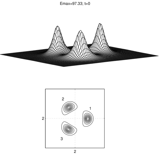
Figure 1: The energy distribution for $N$=3 at the initial time, both in three dimensional and contour plot forms.

Pictures of this energy distribution reveal the familiar $CP^{1}$ lumps, as those of figure 1 for example.

The energy is related to the topological charge by the Bogomolnyi bound

$$E\geq 2\pi|N|.$$ (8)

The instanton solutions correspond to the equality in (8): solutions carrying $N>0$ ($N<0$) imply $\partial_{\bar{z}}W=0$ ($\partial_{z}W=0$), the Cauchy-Riemann conditions for $W$ being an analytic function of $z$ ($\bar{z}$). Note that the simplest non-trivial elliptic function is of order two, hence there are no single-soliton solutions on $T_{2}$.

We utilise the pure model (4) for $N=3$, but for $N=4$ the energy involved is so large that the well-known instability of the planar model (recall its conformal invariance means that the lumps can have any width) breaks the numerical procedure fast. A stabilising Skyrme term must be introduced for this case.

3 Numerical procedure

In this paper we want to discuss time dependent solutions of the model (4) and its Skyrme version [see equation (5)], where the time dependence describes the movement of solitons. As we do not have analytical time-dependent solutions, we resort to numerical simulations. For this we take fields of the form (6) as the initial conditions. Since during the simulations the field $W$ may become arbitrarily large, we have preferred to run our simulations in the $\phi$-formulation of the model. One returns to the $CP^{1}$ formulation inverting (3): $W=(1-\phi_{3})/(\phi_{1}+i\phi_{2})$.

Strictly speaking, truly independent solitons can only be obtained in the asymptotic regime of large soliton separation, which really never happens on a compact manifold such as $T_{2}$. However, each factor $W_{j}\equiv\sigma(z-a_{j})/\sigma(z-b_{j})$ in (6) (when $a_{j}\sim b_{j}$) roughly represents one soliton, providing a setting to studying more or less independent structures. The present work is limited to systems in the topological classes 3 and 4. These systems move, collide and scatter off upon being set into motion by boosting each $W_{j}$ separately. The initial-value problem is then completely specified by giving both $W(t)$ and $\partial_{t}W(t)$ at the initial time $t=0$.

For a square torus we have the so-called lemniscatic case [10] where $\sigma$ posseses the simple Laurent expansion

$$\sigma(u)=\sum_{j=0}^{\infty}{G}_{j}u^{4j+1},\qquad G_{j}\equiv G_{j}(L)\in\Re.$$ (9)

For the accuracy of our calculations it is sufficient to compute the series (9) up to $G_{5}$ (our coefficients for $j>5$ are negligible):

$$\left.\begin{array}[]{lll}G_{0}&=&1\\ G_{1}&=&-0.7878030\\ G_{2}&=&-0.221654845\\ G_{3}&=&9.36193\times 10^{-3}\\ G_{4}&=&7.20830\times 10^{-5}\\ G_{5}&=&2.37710\times 10^{-5}\end{array}\right\}.$$

We have employed the fourth-order Runge-Kutta method and approximated the spatial derivatives by finite differences. The Laplacian has been evaluated using the standard nine-point formula and, to further check our results, a 13-point recipe has also been used. Respectively, the Laplacians are:

$$\nabla^{2}=\frac{\left[\begin{array}[]{cccc}1&4&1\\ 4&-20&4\\ 1&4&1\end{array}\right]}{6\times(\delta x)^{2}},\qquad\nabla^{2}=\frac{\left[\begin{array}[]{ccccc}&&-1&&\\ &1&12&1&\\ -1&12&-48&12&-1\\ &1&12&1&\\ &&-1&&\end{array}\right]}{10\times(\delta x)^{2}}.$$ (10)

The discrete model has been evolved on a $n_{x}\times n_{y}=200\times 200$ square periodic lattice with spatial and time steps $\delta x$=$\delta y$=0.02 and $\delta t$=0.005, respectively. The vertices of the fundamental period cell we have used for our simulations were at

$$(0,0),\;(0,L),\;(L,L),\;(L,0),\quad L=n_{x}\times\delta x=4.$$ (11)

Unavoidable round-off errors have gradually shifted the fields away from the constraint $\vec{\phi}.\vec{\phi}=1$. So, like in the planar case [11], to correct for this we have rescaled $\vec{\phi}\rightarrow\vec{\phi}/\sqrt{\vec{\phi}.\vec{\phi}}$ every few iterations. Each time, just before the rescaling operation, we have evaluated the quantity $\mu\equiv\vec{\phi}.\vec{\phi}-1$  at each lattice point. Treating the maximum of the absolute value of $\mu$ as a measure of the numerical errors, we have found that max$|\mu|$ $\approx$ 10^-8. This magnitude is useful as a guide to determine how reliable a given numerical outcome is. Usage of unsound numerics in the Runge-Kutta evolution shows itself as a rapid growth of max$|\mu|$; this also occurs, for instance, when the solitons pinch-off.

The parameter $\lambda$ in (6) has been set to $\lambda=(1,0)$ all throughout.

4 Three solitons

First we have considered states with three solitons. Our initial configuration is given by taking $\kappa=3$ in (6), the elliptic function of order 3

$$W=\frac{\sigma(z-a_{1})}{\sigma(z-b_{1})}\frac{\sigma(z-a_{2})}{\sigma(z-b_{2})}\frac{\sigma(z-a_{3})}{\sigma(z-b_{3})},\quad\sum_{j=1}^{3}a_{j}=\sum_{j=1}^{3}b_{j}.$$ (12)

The values of $a_{j},b_{j}$ have been selected in such a way that the solitons lie symmetrically around a circle in the network (11). This is easily achieved by fixing $a_{1},b_{1}$ to reasonable values and setting

$$\left.\begin{array}[]{lll}a^{\prime}_{1}&=&a_{1}-c\\ b^{\prime}_{1}&=&b_{1}-c\end{array}\right\},$$ (13)

where $c=(2,2)$ stands for the centre of the period cell. Then

$$\left.\begin{array}[]{lll}a^{\prime}_{j}&=&a^{\prime}_{1}\exp{(i\beta_{j})}\\ b^{\prime}_{j}&=&b^{\prime}_{1}\exp{(i\beta_{j})}\end{array}\right\};\quad\beta_{j}=(j-1)\frac{2\pi}{3},\;j=1,2,3.$$ (14)

This symmetrical arrangement gives solitons of the same size, and satisfies the selection rule in (12) for any choice of the complex numbers $a^{\prime}_{1},\,b^{\prime}_{1}$:

$$\sum_{\kappa=1}^{3}a^{\prime}_{j} = (0,0)$$ (15)

$$= \sum_{\kappa=1}^{3}b^{\prime}_{j}.$$

Next we go back to $a_{j}$ and $b_{j}$ through

$$\left.\begin{array}[]{lll}a_{j}&=&a^{\prime}_{j}+c\\ b_{j}&=&b^{\prime}_{j}+c\end{array}\right.$$ (16)

and supply the system with an initial speed $v_{0}$ by boosting

$$\left.\begin{array}[]{lll}a_{j}&\rightarrow&a_{j}+v_{j}t\\ b_{j}&\rightarrow&b_{j}+v_{j}t\end{array}\right\};\quad v_{j}=-v_{0}\exp{(i\beta_{j})}.$$ (17)

It is now possible to evaluate the time derivative of $W$ at the initial time. Inserting (17) into (12) we get

$$\partial_{t}W(t)\mid_{t=0}=-\prod_{j=1}^{3}v_{j}[\frac{\partial_{z}\sigma(z-a_{j})}{\sigma(z-a_{j})}-\frac{\partial_{z}\sigma(z-b_{j})}{\sigma(z-b_{j})}]W_{j},$$ (18)

where $W_{j}\equiv\sigma(z-a_{j})/\sigma(z-b_{j})$ denotes the $j$-th soliton. Our initial-value problem is defined by (12) and (18).

Choosing

$$\left.\begin{array}[]{lll}a_{1}=(3,2)\\ b_{1}=(1.45,1.95)\\ v_{0}=0.35\end{array}\right\},$$ (19)

gives an initial configuration whose energy density is exhibited in figure 1. The solitons are placed on the vertices of an equilateral triangle; the first lump is situated along the line $y$=2 at $\beta_{1}=0^{\circ}$, with respect to which solitons 2 and 3 are rotated $\beta_{2}=120^{\circ}$ and $\beta_{3}=240^{\circ}$, respectively. These angles are readily checked from the picture with the help of a protractor.

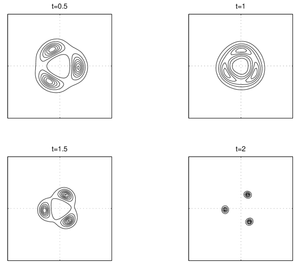
Figure 2: The evolution of the three lumps of figure 1 at various times.

The results of simulations for this case are depicted in figure 2 for various times. The three solitons are fired towards the centre of the triangle and in so doing they expand: the peak $E_{max}$ of the energy density decreases. The solitonic trio collides head-on and coalesces in a ringish structure, then emerging towards the vertices of the dual triangle, that is, the initial line of approach of a given incoming soliton forms an angle of $\pi/3$ with the line along which an outgoing, emerging soliton progresses. This $\pi/3$ scattering can be best appreciated in figure 3, where both the initial state ($t$=0) and the final state ($t=2$) are displayed together.

Returning to figure 2 we see that $E_{max}$ becomes narrower with time, particularly after the lumps scatter off and start drawing away from each other. At $t=2$, for instance, the maximum value of the energy density goes up to $E_{max}=579.37$. Soon after $t>2$ this peak gets so spiky that the numerics breaks down: the instability of the planar $O(3)$ model takes over and leads to singularity formation.

Our result is noteworthy: the initial configuration, although positioned at the vertices of an equilateral triangle in the period cell, does not produce $D_{3}$ symmetry because the torus itself, being homogeneous but not isotropic, has no such symmetry (the fundamental grid has directed sides). One could reasonably expect the lumps to scatter along directions that need not respect $D_{3}$ symmetry. Therefore, the rationale applied to explain $\pi/N$ scattering for the model on $\Re_{2}$ is no longer valid for the model with periodic boundary conditions.

However, we observe that as the solitons are well localised the boundary conditions may not be very important. Note that our numerical results are consistent with this expectation. To test this further we could place our solitons nearer the edges of the grid and see whether we still observe the 60⁰ scattering. We hope to investigate this issue in the future.

5 Four solitons

Next we have looked at the $N=4$ configurations. The initial field is given by the elliptic function of order 4

$$W=\frac{\sigma(z-a_{1})}{\sigma(z-b_{1})}\frac{\sigma(z-a_{2})}{\sigma(z-b_{2})}\frac{\sigma(z-a_{3})}{\sigma(z-b_{3})}\frac{\sigma(z-a_{4})}{\sigma(z-b_{4})},\quad\sum_{j=1}^{4}a_{j}=\sum_{j=1}^{4}b_{j},$$ (20)

where $a_{j},b_{j}$ are chosen so that the solitons sit symmetrically at the vertices of a square in the basic cell. A treatment parallel to that of the previous section leads to

$$\left.\begin{array}[]{lll}a^{\prime}_{j}&=&a^{\prime}_{1}\exp{(i\varphi_{j})}\\ b^{\prime}_{j}&=&b^{\prime}_{1}\exp{(i\varphi_{j})}\end{array}\right\};\quad\varphi_{j}=(j-1)\frac{\pi}{2},\;j=1,2,3,4,$$ (21)

The condition between the zeros and poles is again verified $\forall\;a^{\prime}_{1},\,b^{\prime}_{1}$ :

$$\quad\sum_{j=1}^{4}a^{\prime}_{j} = (0,0)$$

$$= \sum_{j=1}^{4}b^{\prime}_{j}.$$

Both the initial velocity and the time dependence are introduced by boosting:

$$\left.\begin{array}[]{lll}a_{j}&\rightarrow&a_{j}+v_{j}t\\ b_{j}&\rightarrow&b_{j}+v_{j}t\end{array}\right\};\quad v_{j}=-v_{0}\exp{(i\varphi_{j})},$$ (22)

where equation (16) should be kept in mind.

As pointed out in section 2, four lumps involve a large energy and while evolving in time they become too spiky before we can learn anything much about the scattering process. We have therefore studied this system in the Skyrme version of the theory, where the solitons are stable and may be examined for as long as required.

Instead of the Lagrangian density (4) we have thus taken:

$${\cal L}=\frac{|W_{t}|^{2}-2|W_{z}|^{2}-2|W_{\bar{z}}|^{2}}{(1+|W|^{2})^{2}}\\ -8\theta_{1}\frac{|W_{z}|^{2}-|W_{\bar{z}}|^{2}}{(1+|W|^{2})^{4}}(|W_{t}|^{2}+|W_{z}|^{2}-|W_{\bar{z}}|^{2}).$$

The configuration (6) is no longer an exact solution of the field equation derived from (5), albeit it is a very good approximation to it. We should also stress that the presence of a Skyrme term does not affect the trajectory of the lumps before the collision or their scattering angle.

Taking

$$\left.\begin{array}[]{lll}a_{1}=(2.05,2.55)\\ b_{1}=(2.95,2.95)\\ \theta_{1}=10^{-3}\\ v_{0}=0.35\exp(i\pi/4)\end{array}\right\},$$ (23)

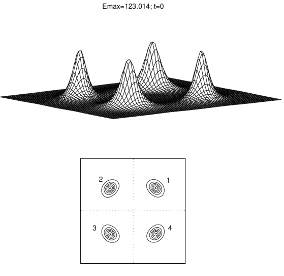
Figure 4: The energy distribution for $N$=4 at $t=0$.

entails the state of identical ‘baby skyrmions’ illustrated in figure 4. The solitons $W_{2}$, $W_{3}$ and $W_{4}$ are rotated $90^{\circ},180^{\circ}$ and $270^{\circ}$ with respect to $W_{1}$, which we have conveniently placed in the first quadrant, roughly on the central diagonal joining the grid points (0,0)-(4,4).

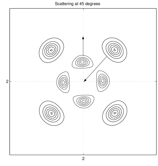
Figure 6: Scattering at $\pi/4$ radians.

The system (20) gets moving via (22) and zeroes in on the middle of the mesh, where the four skyrmions bump head-on into each other. This dynamics makes the solitons scatter off and emerge towards the vertices of the dual square, emerging at $45^{\circ}$ with respect to the initial direction of motion, as depicted in diagram 5. Figure 6 superimposes both the initial state ($t$=0) and the final state ($t=3$), allowing greater clarity in the appreciation of the scattering angle $\pi/4$.

Unlike the outcome of the previous section, the dual square scattering on $T_{2}$ is not so surprising. For although the initial data doesn’t have $D_{4}$ symmetry, it does have 4-fold rotational symmetry and zero angular momentum. Note that the boundary conditions (5) break the $SO(2)$ rotational symmetry of the plane into a 4-fold rotational symmetry.

6 Geodesic approximation

Note that, in analogy to the $S_{2}$ case, when $v$ in (17) and (22) is set to zero our initial configuration is a static solution of the equations of motion. If we change $a_{j}$, $b_{j}$ to a new value given by (17) or (22) for a particular value of $t$ the new configuration is again a static solution of the equations of motion. Hence as $v$ changes the changes (17) and (22) connect configurations which correspond to static solutions of the equations of motion. Thus it is reasonable to expect that a system set off with a small $v$ will follow such a change. This expectation goes under the name of geodesic approximation (the system evolves by changing its zero-mode parameters). Its validity is not expected to depend too much on whether the model is defined on $S_{2}$ or $T_{2}$.

So far we have been concerned with solitons of equal size. Let us now look into the more general and interesting situation of energy lumps of different sizes, illustrating the proceedings by studying the case $N=3$.

First we set up the initial configuration and evolve it through our standard numerical simulation. Then we choose a set of collective coordinates to reproduce the results of our simulations (trajectory, scattering), offering an explanation in the framework of the geodesic approximation.

6.1 Numerical simulation

Our 3-soliton system is still given by a function of the form (12), but with a layout not as symmetrical as before. Instead of (14) we put

$$\left.\begin{array}[]{lll}a^{\prime}_{j}&=&a^{\prime}_{1}\exp{(i\alpha_{j})}\\ b^{\prime}_{j}&=&b^{\prime}_{1}\exp{(i\alpha_{j})}\end{array}\right\};\quad\alpha_{j}=(j-1)\frac{2\pi}{3}+(-1)^{(j-1)}(1-\delta_{1j})\xi,$$ (24)

with $j$=1,2,3 and the numbers $a^{\prime}_{1},\;b^{\prime}_{1}$ being fixed as customary. The initial three soliton configuration can be written as

$$W = \frac{\sigma(z-a_{1})}{\sigma(z-b)}\frac{\sigma(z-a_{2})}{\sigma(z-b_{2})}\frac{\sigma(z-a_{3})}{\sigma(z-b_{3})}$$ (25)

$$= \frac{\sigma(z^{\prime}-a^{\prime}_{1})}{\sigma(z^{\prime}-b^{\prime})}\frac{\sigma(z^{\prime}-a^{\prime}_{1}e^{i\alpha_{2}})}{\sigma(z^{\prime}-b^{\prime}_{1}e^{i\alpha_{2}})}\frac{\sigma(z^{\prime}-a^{\prime}_{1}e^{-i\alpha_{2}})}{\sigma(z^{\prime}-b^{\prime}_{1}e^{-i\alpha_{2}})},$$

where

$$b^{\prime}=a^{\prime}_{1}+2(a^{\prime}_{1}-b^{\prime}_{1})\cos\alpha_{2}\quad[\alpha_{2}=\frac{2\pi}{3}-\xi]$$ (26)

ensures that the zeros and poles in (25) comply with the constraint in (6). As usual we switch between primed and unprimed numbers through formula (16), plus $b^{\prime}=b-c$ and $z^{\prime}=z-c$. We have also used the fact that $\exp(i\alpha_{3})=\exp(-i\alpha_{2})$.

Note that equating $\xi$ to zero simplifies $\alpha_{j}$ to $(j-1)2\pi/3=\beta_{j}=$ of (14), whereupon the elliptic function (25) reduces to the field (12) simply because $\cos\alpha_{2}=\cos\beta_{2}=-1/2\rightarrow b^{\prime}=b^{\prime}_{1}$ according to (26).

An angle $\xi\neq 0$ generates solitons of different sizes which no longer enjoy the positional symmetry boasted by the arrangement (14). In the set-up (14), where $\xi$=0 and the solitons have the same size, the required relationship $\sum a^{\prime}_{j}=\sum b^{\prime}_{j}$ looks after itself as shown in (15). For $\xi\neq 0$ a demand of the kind (26) is needed.

Now we have evolved the solitons (25) in the pure version of the $CP^{1}$ model, with the solitons being sent into collision in the regular fashion:

$$\left.\begin{array}[]{lll}a_{j}&\rightarrow&(a^{\prime}_{1}-v_{0}t)\exp{(i\alpha_{j})}+c\\ b&\rightarrow&(b^{\prime}-v_{0}t)+c\\ b_{s}&\rightarrow&(b^{\prime}_{1}-v_{0}t)\exp{(i\alpha_{s})}+c\\ \end{array}\right\};\quad j=1,2,3;\;\;s=2,3.$$ (27)

The associated energy distribution is shown for a typical case by the contour plot of figure 7, which corresponds to a choice of parameters (19) in addition to $\xi=10^{\circ}$.

The starting configuration is represented by the three wider structures whereas the final, scattered state is the narrower trio plotted therein. The sense of motion is clearly indicated by the arrows. We note that for both configurations the solitons are rotated an extra angle $\xi$ with respect to $W_{1}$, as compared to their partners of figure 3, And, unlike the latter, it is not the case that the three initial lumps have the same size; nor they are situated at the vertices of an equilateral triangle. Apparent as well from our simulations is that the scattering angle differs from $\pi/3$. This is a consequence of considering nonsymmetrical solitons, whose collisions are not elastic and thus involve energy transfer.

Clearly the distance between the solitons differ for different pairs of them and so their interactions are not the same resulting in a different scattering pattern. Can we explain this difference? In the next subsection we show that an explanation can be provided in terms of, appropriately chosen, collective coordinates and the motion following appropriate geodesics.

6.2 Collective coordinates

In order to make a wise selection of collective coordinates let us consider closely the positions and sizes of the solitons defined in the previos subsection.

The location of the solitons (25) are clearly given by

$${a^{\prime}_{1}+b^{\prime}\over 2},\quad{a^{\prime}_{1}+b^{\prime}_{1}\over 2}e^{i\alpha_{2}},\quad{a^{\prime}_{1}+b^{\prime}_{1}\over 2}e^{-i\alpha_{2}},$$ (28)

and their sizes are

$$|{a^{\prime}_{1}-b^{\prime}\over 2}|,\quad|{a^{\prime}_{1}-b^{\prime}_{1}\over 2}|,\quad|{a^{\prime}_{1}-b^{\prime}_{1}\over 2}|.$$ (29)

Put

$$a^{\prime}_{1}=k-\chi,\;b^{\prime}_{1}=k+\chi$$ (30)

so the positions (28) adopt the form

$$k-\chi[1+2\cos(\alpha_{2})],\quad ke^{i\alpha_{2}},\quad ke^{-i\alpha_{2}},$$ (31)

while the sizes (29) read

$$|2\chi\cos(\alpha_{2})|,\quad|\chi|,\quad|\chi|.$$ (32)

Consistently, for $\xi=0$ the description (31)-(32) corresponds to objects of the same size $|\chi|$ which are symmetrically situated at $k$ and $k\exp({\pm i2\pi/3})$ (with respect to the centre). For simplicity, we have taken two lumps with the same size and a third lump with a different size.

A possible collective coordinate description involves treating $k$, $\chi$ and $\alpha_{2}$ as collective coordinates. Thus, in the simulation we expect $\alpha_{2}$ and $\chi$ to remain approximately constant and $k$ to vary. We are suggesting that the scattering can be understood as proceeding (on average) with only $k$ depending on time and varying from (take $k$ real for simplicity) $k>0$ to $k<0$. It is easy to show, although a bit tedious in practice (this involves estimating various elliptic integrals which can be done partially analytically, partially numerically), that both on $\Re_{2}$ or on our torus the kinetic energy of the motion just described is finite. So such a behaviour is possible.

We have carried out our collective coordinates “motion” using the specific values

$$\chi=(0.55,0),\quad k=(u,0),\;u\in[1,-1],$$ (33)

where $u$ varies across the interval in steps of 0.2. We see from (31) and (33) that the configurations for $u>0$ ($u<0$) correspond to incoming (outgoing/scattered) lumps. The value $u\approx 0$ represents the situation where the solitons have collided and are on top of each other, coalescing in the centre of the mesh. It is largely the behaviour of $W$ at $u\approx 0$ what determines the scattering angle.

The state for $k$=(1,0) (incoming lumps) and $k$=(-0.2,0) (“scattered” lumps) are depicted in figure 8 for the case $\xi=10^{\circ}$. As long as the path followed by the lumps and the scattering angle is concerned, the similarity with the numerically evolved situation of figure 7 is clear. We stress that since we are mostly interested in the relative position of the solitons and their scattering angles, it is immaterial that the breadths of the solitons in figure 7 differ from the solitons of figure 8.

A more detailed comparison can be made by viewing a trajectory plot, one showing consecutive snapshots [corresponding to $k$=(1,0), (0.8,0),…,(-0,2),(-0.4,0)…(-1,0)] of lump positions as they approach each other and scatter off.

This is shown in figure 9, where the full collective coordinate motion has been ticked with small circles and the motion according to the time evolution of subsection 6.1 has been sketched with solid lines. Note that after scattering the path of the numerically evolved lumps (continuos lines) cannot be followed much farther; this is because the solitons get very spiky and the simulation breaks down.

Our simulations have been carried out for several values of $\xi$ and have been compared with the corresponding collective coordinate motion. We have always found the trajectories from both approaches to be in agreement, thus supporting our choice of collective coordinates. Another illustration is provided by figure 10 for the case $\xi=20^{\circ}$.

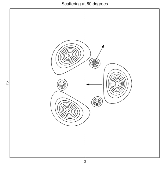
Figure 3: Scattering at $\pi/3$ radians.

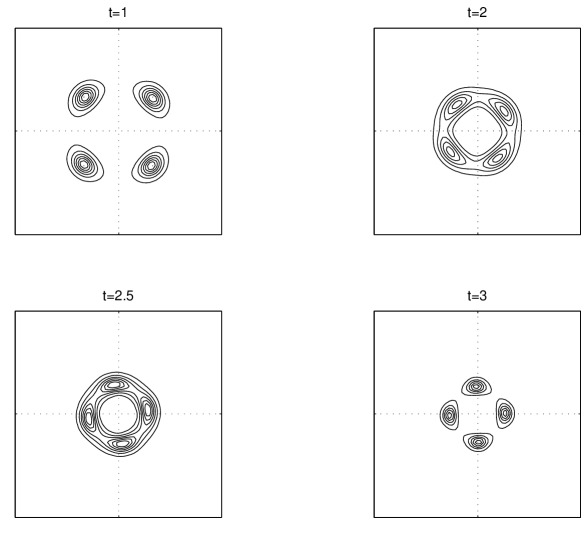
Figure 5: The evolution of the four lumps of figure 4 gets underway.

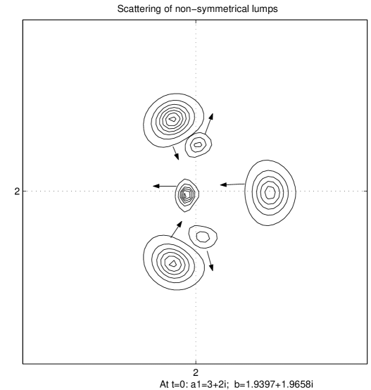
Figure 7: Numerical simulation for solitons rotated an angle $\xi=10^{\circ}$ with respect to the symmetrical configuration of figure 1. They do not scatter at $60^{\circ}$.

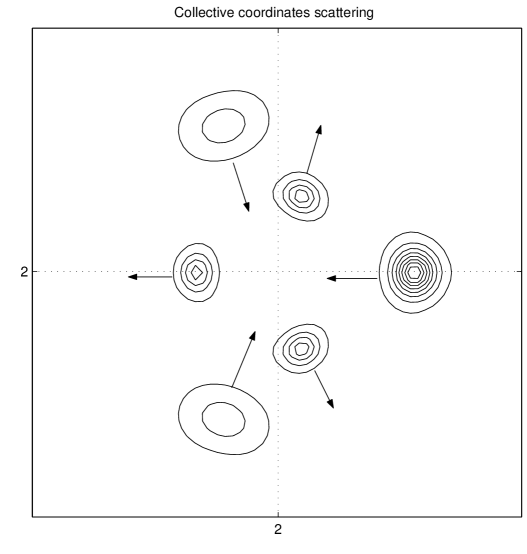
Figure 8: “Scattering” according to our collective coordinates view for $\xi=10^{\circ}$, to be compared with the numerical result shown in figure 7. The incoming lumps are pictured for $k=(1,0)$ and the outgoing structures correspond to $k=(-0.2,0)$. It is not important that the widths of these lumps are not the same as their sibblings of figure 7: we worry about the relative positions and scattering angle.

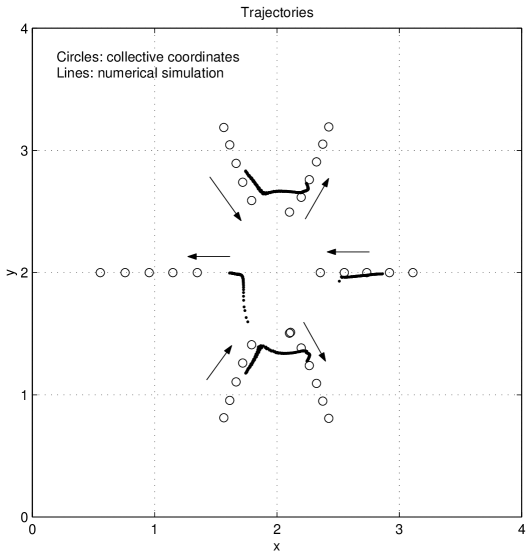
Figure 9: Trajectory plots ($\xi=10^{\circ}$) sketching the path followed by the humps presented in figures 7 and 8. The itinerary according to our geodesic approximation (circles) shows very good agreement with the motion obtained via numerical simulation (solid lines).

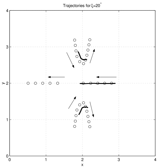
Figure 10: Plots comparing the trajectory obtained via numerical simulations (solid lines) and the trajectory gotten using the geodesic approximation (circles) for $\xi=20^{\circ}$.

7 Conclusions

In this article we have studied head-on collisions between solitons in the (2+1)-D $CP^{1}$ model with periodic boundary conditions, that is, with the model defined on a flat torus $T_{2}$.

Through numerical simulations we have found that solitons of equal sizes (at the initial time) scatter at an angle $\pi/N$, or dual-polygon scattering, where $N$ is the soliton number or topological charge of the system. In this paper we have focused on $N=3,4$ (the case $N=2$ has been considered previously [4] and it has been found to comply with the $\pi/2$ scattering).

Unlike the usual model on $\Re_{2}$, our model with periodic boundary conditions breaks the $SO(2)$ rotational invariance of the plane, leaving us with a numerical mesh with directed sides where the initial soliton configuration has no symmetry under the dihedral group $D_{N}$. So it is remarkable to still find dual-triangle scattering in this format. On the other hand, since the $SO(2)$ symmetry breaks into a four-fold rotational symmetry, the dual-square scattering is less unexpected.

We have also considered solitons of different sizes (at the initial time) and have observed that the scattering angle in no longer $\pi/N$, outcome arising from the fact that there is energy transfer in collisions between unsymmetrical solitons.

By reparametrising the quantities describing the positions of the solitons using a juditious set of collective coordinates, we have been able to reproduce the above numerical results, thus offering an explanation of the scattering process. We have illustrated this approach using a 3-soliton field.

These results raise important questions pertaining to the the interplay between the symmetry of the initial configuration and the lack of symmetry of the torus itself. As pointed out at the end of section 4, the non-isotropy of the torus might affect the evolution of the lumps if they are initially placed near the boundary of the mesh. What about systems with $N$=5,6,…? Numerical experiments on a periodic, rectangular grid would also be worth performing. We hope to report on these matters in the near future.

Acknowledgements

Work for this paper was carried out during the authors’ visits to Durham and Maracaibo, supported by the ROYAL SOCIETY, CONICIT and LUZ-CONDES. The paper was completed at IISC, Bangalore-India, where $\Re$J Cova stayed thanks to a grant TWAS-UNESCO. He thanks Prof Uberoi and Prof Rangarajan for their hospitality at IISc.

References

- [1] Proc. Physics in (2+1) dimensions (Korea), World Scientific (1992)
- [2] Leese RA et al Nonlinearity 3, 387 (1990)
- [3] Skyrme THR Nucl Phys 31, 556 (1962)
- [4] Cova RJ and Zakrzewski WJ Nonlinearity 10, 1305 (1997)
- [5] Speight JM Comm Math Phys 194, 513 (1998)
- [6] Cova RJ Eur Phys Jour B 23, 201 (2001)
- [7] Kudryavtsev A, Piette B and Zakrzewski W Phys Lett A 183, 119 (1993)
- [8] Goursat E Functions of a complex variable, Dover Publications (1916)
- [9] Lawden DF Elliptic functions and applications Springer Verlag (1989)
- [10] Erdélyi A et al Higher transcendental functions vol II Mc Graw Hill (1953).
- [11] Piette B and Zakrzewski W Chaos, solitons and fractals 5, 2495 (1995)