Braneworld cosmological models with anisotropy

Abstract

For a cosmological Randall-Sundrum braneworld with anisotropy, i.e., of Bianchi type, the modified Einstein equations on the brane include components of the five-dimensional Weyl tensor for which there are no evolution equations on the brane. If the bulk field equations are not solved, this Weyl term remains unknown, and many previous studies have simply prescribed it ad hoc. We construct a family of Bianchi braneworlds with anisotropy by solving the five-dimensional field equations in the bulk. We analyze the cosmological dynamics on the brane, including the Weyl term, and shed light on the relation between anisotropy on the brane and Weyl curvature in the bulk. In these models, it is not possible to achieve geometric anisotropy for a perfect fluid or scalar field – the junction conditions require anisotropic stress on the brane. But the solutions can isotropize and approach a Friedmann brane in an anti-de Sitter bulk.

I Introduction

High-energy physics theories have recently inspired relatively simple phenomenological models in which one can test some of the consequences of string theories. Randall and Sundrum Randall and Sundrum (1999a, b) proposed a model that captures some of the essential features of the dimensional reduction of eleven-dimensional supergravity introduced by Ho$\check{\mbox{r}}$ava and Witten Horava and Witten (1996a, b). The second Randall-Sundrum (RS2) scenario Randall and Sundrum (1999b) is a five-dimensional Anti-de Sitter ($AdS_{5}$) “bulk” spacetime with an embedded Minkowski 3-brane where matter fields are confined and Newtonian gravity is effectively reproduced at low energies. The RS2 scenario was generalized to a Friedmann-Robertson-Walker (FRW) brane, showing that the Friedmann equation at high energies gives $H^{2}\sim\rho^{2}$, in contrast with the general-relativistic behaviour $H^{2}\sim\rho$ Binetruy et al. (2000a, b); Csaki et al. (1999); Cline et al. (1999).

As shown in Shiromizu et al. (2000), the modified field equations on the brane have two new contributions from extra-dimensional gravity:

$$G_{\alpha\beta}=-\Lambda g_{\alpha\beta}+\kappa^{2}T_{\alpha\beta}+6{\kappa^{2}\over\lambda}{\cal S}_{\alpha\beta}-{\cal E}_{\alpha\beta}\,,$$ (1)

where $\lambda$ is the brane tension (the vacuum energy of the brane when $T_{\alpha\beta}=0$), and $\Lambda$ and $\kappa$ are the four-dimensional cosmological and gravitational constants respectively, given in terms of $\lambda$ and the fundamental constants of the bulk $(\Lambda_{5}\,,\kappa_{5})$ by:

$$\Lambda={\Lambda_{5}\over 2}+{\lambda^{2}\over 12}\kappa_{5}^{2}\,,~{}\kappa^{2}={\lambda\over 6}\kappa_{5}^{4}\,.$$ (2)

The term ${\cal S}_{\alpha\beta}$ is quadratic in $T_{\alpha\beta}$ and dominates at high energies ($\rho>\lambda$). The five-dimensional Weyl tensor is felt on the brane via its projection, ${\cal E}_{\alpha\beta}$. This Weyl term is determined by the bulk metric, not by equations on the brane. In FRW braneworlds, the bulk is Schwarzschild-$AdS_{5}$ Bowcock et al. (2000); Kraus (1999); Ida (2000), and ${\cal E}_{\alpha\beta}$ reduces to a simple Coulomb term that gives rise to “dark radiation” on the brane. The simplest generalizations of FRW braneworlds are Bianchi braneworlds.

By making an assumption about the Weyl term on the brane, the dynamics of a Bianchi type I brane were studied in Maartens et al. (2001), and it was shown that high-energy effects from extra-dimensional gravity remove the anisotropic behaviour near the singularity that is found in general relativity. This was extended via a phase space analysis of Bianchi I and V braneworlds Campos and Sopuerta (2001a, b), showing that the anisotropy is negligible close to the singularity for perfect fluid models with a barotropic linear equation of state $p=w\rho$, with $w\geq 0$ a constant, opposite to the general relativity case. It was then suggested that this may be generic in cosmological braneworlds, which was supported by subsequent work Coley (2002a, b) (see also Hervik (2003); van den Hoogen et al. (2002); Coley and Hervik (2003)). However, a perturbative analysis Bruni and Dunsby (2002) suggests that this may only be true for homogeneous models.

These studies, and others Santos et al. (2001); Toporensky (2001); Chen et al. (2001a, b); Paul (2001); Barrow and Maartens (2002); Savchenko et al. (2002); Paul (2002); Harko and Mak (2003); van den Hoogen and Ibanez (2003); Aguirregabiria et al. (2003); Aguirregabiria and Lazkoz (2003), considered only the dynamical equations on the brane, making various assumptions about the Weyl term in the absence of knowledge of the bulk metric. In Frolov (2001) a bulk metric with a Kasner brane was presented. However, since the Kasner metric is a solution of the 4-dimensional Einstein vacuum equations, the bulk metric is a simple warped extension; the general result, with the generic form of the bulk metric, is given in Brecher and Perry (2000) . The simplest example of this general result is a Minkowski brane, leading to the RS2 solution. Another example is the Schwarzschild black string solution Chamblin et al. (2000). Up to now, no complete solutions, i.e., for the brane and bulk metrics, have been found for cosmological Bianchi braneworlds . The key difficulty is to find anisotropic generalizations of $AdS_{5}$ that can incorporate anisotropy on a cosmological brane, and that are necessarily non-conformally flat.

Previous studies of Bianchi braneworlds have considered the effects of ${\cal S}_{\alpha\beta}$, under various assumptions on ${\cal E}_{\alpha\beta}$. Here we tackle the question of the construction of complete models for cosmological braneworlds with anisotropy, that is, we want to construct both the metric in the bulk and on the 3-brane, so that ${\cal E}_{\alpha\beta}$ is determined and not assumed ad hoc.

II The geometry of the bulk

For a five-dimensional bulk spacetime with a negative cosmological constant, $\Lambda_{5}<0$, and no additional matter sources, the Einstein equations are:

$${}^{5\!}G_{AB}+\Lambda_{5}\,^{5\!}g_{AB}=0\,.$$ (3)

In order to construct cosmological braneworlds with anisotropy we start from the ansatz used by Binetruy et al. (2000a, b) (see also Mukohyama (2000); Vollick (2001)):

$${}^{5\!}ds^{2}=-n^{2}(t,y)dt^{2}+a^{2}(t,y)d\Sigma^{2}_{k}+b^{2}(t,y)dy^{2}\,,$$ (4)

where $d\Sigma^{2}_{k}$ is the line element of the three-dimensional maximally symmetric surfaces $\{t=t_{\ast},y=y_{\ast}\}$, with curvature curvature index $k=0,\pm 1$. Clearly, all the hypersurfaces $\{y=y_{\ast}\}$ inherit a FRW metric. Although the Einstein equations (3) can be completely solved for the metric (4), the explicit complete solution (bulk+brane) (see Binetruy et al. (2000a, b)) was found for $\dot{b}=0$, which corresponds to Gaussian normal coordinates adapted to the foliation with normal $n_{A}dx^{A}=dy$. Since the bulk is Schwarzschild-$AdS_{5}$, an alternative approach is based on a moving brane in static spherical bulk coordinates Kraus (1999); Ida (2000),

$${}^{5\!}ds^{2}=-f(r)dT^{2}+\frac{dr^{2}}{f(r)}+r^{2}d\Sigma^{2}_{k}\,,$$ (5)

where

$$f(r)=k+\frac{r^{2}}{\ell^{2}}-\frac{\mu}{r^{2}}\,.$$ (6)

Here $\ell^{2}=-6/\Lambda_{5}$, so that $\ell$ is the curvature scale of the bulk. When the parameter $\mu$, the mass of the bulk black hole, vanishes, the solution is simply $AdS_{5}$, so that the bulk Weyl tensor, and hence the brane Weyl term, vanish. If $\mu\neq 0$, then the tidal field of the black hole generates a non-zero Weyl term on the brane. The existence of the black hole horizon requires that $\mu\geq 0$ for a flat or closed geometry, and $\mu\geq-\ell^{2}/4$ for the open case. The brane trajectory is $r=a(\tau)$, where $\tau$ is cosmological proper time on the brane and $a(\tau)$ is the scale factor, whose evolution is determined by the junction conditions. For a $Z_{2}$-symmetric brane, this gives the modified Friedmann equation on the brane,

$$H^{2}+{k\over a^{2}}={\kappa^{2}\over 3}\rho\left(1+{\rho\over 2\lambda}\right)+{\Lambda\over 3}+{\mu\over a^{4}}\,,$$ (7)

where the high-energy correction term is $\rho^{2}/\lambda$ and the last term on the right is the dark radiation term.

A natural extension of the ansatz in Eq. (4) that will introduce anisotropy is (compare Cadeau and Woolgar (2001) for a similar approach):

$${}^{5\!}ds^{2}=-n^{2}(t,y)dt^{2}+h_{IJ}(t,y)\omega^{I}\omega^{J}+b(t,y)^{2}dy^{2}\,,$$ (8)

where $\omega^{I}=\omega^{I}_{i}dx^{i}$ are 1-forms invariant under a Bianchi group (see Stephani et al. (2003) for details), and $h_{IJ}\omega^{I}\omega^{J}$ is the metric induced on the surfaces $\{t=t_{\ast}\,,y=y_{\ast}\}$. For simplicity, we consider only Bianchi type I models ($\omega^{I}_{i}=\delta^{I}_{i}$) (the procedure for non-Abelian Bianchi groups is essentially the same) with a diagonal metric $h_{IJ}$:

$${}^{5\!}ds^{2}=-a^{2}_{0}(t,y)dt^{2}+\sum_{i=1}^{3}a^{2}_{i}(t,y)(dx^{i})^{2}+b(t,y)^{2}dy^{2}\,.$$ (9)

The field equations (3) for this metric are non-linear partial differential equations (PDEs) in $(t,y)$, like the field equations for the metric (4). In the case of the metric (4) the $\{ty\}$-component of the field equations provides a relation that leads to a set of first integrals. However, this procedure does not work for Eq. (9), and one must deal with non-linear PDEs. We have not been able to find a procedure to solve them analytically.

These difficulties indicate that in order to find analytic solutions we should abandon the generic case and consider special solutions that do not require PDEs. We try a static and Gaussian normal ansatz,

$${}^{5\!}ds^{2}=-e^{2A_{0}(y)}dt^{2}+\sum^{3}_{i=1}e^{2A_{i}(y)}(dx^{i})^{2}+dy^{2}\,,$$ (10)

where we pay the price that the brane is no longer static in the coordinate system. This ansatz can in fact be seen as a five-dimensional generalization of a similar ansatz Linet (1986) used in the search for four-dimensional static and cylindrically symmetric spacetimes describing cosmic strings in the presence of a non-vanishing cosmological constant. The field equations for the metric (10) are

$$A^{\prime\prime}_{\alpha}+A^{\prime}_{\alpha}\sum^{3}_{\beta=0}A^{\prime}_{\beta}-\frac{\omega^{2}}{4} = 0\,,$$ (11)

$$\sum_{0\leq\alpha<\beta\leq 3}\!\!\!A^{\prime}_{\alpha}A^{\prime}_{\beta}-\frac{3}{8}\omega^{2} = 0\,,$$ (12)

where $\omega=4/\ell$.

In order to solve these equations, we introduce the determinant of the metric,

$$u^{2}(y)=\exp\left(2\sum_{\alpha=0}^{3}A_{\alpha}\right)\,.$$ (13)

Multiplying Eq. (11) by $u(y)$ and summing over $\alpha$, we get

$$u^{\prime\prime}-\omega^{2}u=0\,,$$ (14)

with first integral,

$$u^{\prime 2}-\omega^{2}u^{2}+C=0\,,$$ (15)

where $C$ is an arbitrary constant of integration. Once $u(y)$ is known, $A_{\alpha}(y)$ can be obtained by quadrature:

$$A^{\prime}_{\alpha}=\frac{1}{4}\frac{u^{\prime}}{u}+\frac{C_{\alpha}}{u}\,,$$ (16)

which comes from the integration of Eq. (11). The constants $C_{\alpha}$ are constrained by Eqs. (12) and (13):

$$\sum^{3}_{\alpha=0}C_{\alpha} = 0\,,$$ (17)

$$\sum_{0\leq\alpha<\beta\leq 3}C_{\alpha}C_{\beta} = \frac{3}{8}C\,.$$ (18)

These imply

$$(C_{1}+C_{2})^{2}+(C_{1}+C_{3})^{2}+(C_{2}+C_{3})^{2}=-\frac{3}{4}C\,.$$ (19)

Taking the square of Eq. (17) and using Eq. (18) yields equivalently

$$\sum_{\alpha=0}^{3}C^{2}_{\alpha}=-\frac{3}{4}C\,.$$ (20)

Thus $C$ can never be positive, and the $C_{\alpha}$’s must be the coordinates of a three-sphere of radius $\sqrt{-3C}/2$, hence $|C_{\alpha}|\leq\sqrt{-3C}/2$.

When $C=0$ the parameters $C_{\alpha}$ must all be zero as well. In this particular case,

$$A_{\alpha}(y)=A^{o}_{\alpha}+\frac{\omega}{4}(y-y_{o})\,,$$ (21)

where $A^{o}_{\alpha}$ are integration constants. This model corresponds, as expected, to an exact $AdS_{5}$ bulk.

Thus, we are left to consider negative values for $C$, and we rewrite it as $C=-\omega^{2}B^{2}$. By Eq. (15),

$$u(y)=B\sinh\left[\omega(y-y_{o})\right]\,,$$ (22)

and then Eq. (16) gives

$$A_{\alpha}(y)=A^{o}_{\alpha}+\frac{1}{4}\ln\left|u(y)\right|+C_{\alpha}v(y)\,,$$ (23)

where $v^{\prime}=1/u$, so that

$$v(y)=\frac{1}{2\omega B}\ln\left\{\frac{\cosh\left[\omega(y-y_{o})\right]-1}{\cosh\left[\omega(y-y_{o})\right]+1}\right\}\,.$$ (24)

Finally, we can write the bulk metric solution as

$$e^{2A_{\alpha}} = N^{2}_{\alpha}\big{|}\sinh\left[\omega(y-y_{o})\right]\big{|}^{1/2}$$ (25)

$$~{}{}\times\left\{\frac{\cosh\left[\omega(y-y_{o})\right]-1}{\cosh\left[\omega(y-y_{o})\right]+1}\right\}^{q_{\alpha}}\,,$$

where $q_{\alpha}=C_{\alpha}/\omega B$ (recall that $\omega B\neq 0$), and $N_{\alpha}$ are constants whose value can be chosen by rescaling coordinates, but which satisfy the constraint

$$\prod_{\alpha=0}^{3}N^{2}_{\alpha}=B^{2}\,,$$ (26)

which follows from Eqs. (13) and (22). The exponents $q_{\alpha}$ are constrained by Eqs. (17) and (20):

$$\left|q_{\alpha}\right|~{}\leq~{}\frac{3}{4}\,.$$ (27)

Note that this is a more restrictive bound than the one found above only from Eq. (20).

We consider first the special case $C_{1}=C_{2}=C_{3}=-C_{0}/3$, with two possible sets of parameters in Eq. (25), namely $(q^{\pm}_{0},q^{\pm}_{i})=(\mp{3\over 4},\pm{1\over 4})$. These two special cases are Schwarzschild-$AdS_{5}$, with $k=0$, written in Gaussian normal coordinates. (The $k=-1$ case corresponds to Bianchi V, and the $k=1$ case to Bianchi IX.) We see this via a coordinate transformation in the metric of Eq. (5):

$$r^{4}=\frac{8\mu}{\omega^{2}}(1\mp\cosh\left[\omega(y-y_{o})\right])\,,$$ (28)

and the remaining coordinates are rescaled by constants that depend on $\mu$, $\omega$, and $N_{\alpha}$. It follows that $q^{+}_{\alpha}$ leads to a negative mass $\mu$, which we exclude, so that $q^{-}_{\alpha}$ is the physical solution (with a black hole horizon).

This shows that our general five-dimensional bulk solution, Eq. (25), can be seen as an anisotropic generalisation of Schwarzschild-$AdS_{5}$. This distinguishes our anisotropic solution from the vacuum Kasner braneworld Frolov (2001).

We now investigate the character of the singular point $y=y_{o}$ via curvature scalars. It turns out to be more convenient to use a new set of constants,

$$\frac{d_{1}}{2}=q_{2}+q_{3}\,,~{}\frac{d_{2}}{2}=q_{1}+q_{3}\,,~{}\frac{d_{3}}{2}=q_{1}+q_{2}\,,$$ (29)

with

$$d^{2}_{1}+d^{2}_{2}+d^{2}_{3}=3\,.$$ (30)

The isotropic cases $q^{\pm}_{\alpha}$ correspond to the points $(\pm 1,\pm 1,\pm 1)$ on the 2-sphere (30). The square of the bulk Weyl tensor, ${\cal C}^{2}=\,^{5\!}C_{ABCD}\,^{5\!}C^{ABCD}$ is given by

$${\cal C}^{2} = \frac{\omega^{4}}{16\sinh^{4}[\omega(y-y_{o})]}\left\{21-\left(d^{4}_{1}+d^{4}_{2}+d^{4}_{3}\right)\right.$$ (31)

$$\left.~{}{}+18\cosh^{2}[\omega(y-y_{o})]\right.$$

$$\left.~{}{}+36d_{1}d_{2}d_{3}\cosh[\omega(y-y_{o})]\right\}\,.$$

The behaviour near $y_{o}$ is

$${\cal C}^{2}\underset{y\rightarrow y_{o}}{\longrightarrow}~{}\frac{\left[39+36\,d_{1}d_{2}d_{3}-\left(d^{4}_{1}+d^{4}_{2}+d^{4}_{3}\right)\right]}{16(y-y_{o})^{4}}\,.$$ (32)

There are four sets of constants $d_{i}$ that lead to zero numerator: $D_{1}=(-1,1,1)\,,$ $D_{2}=(1,-1,1)\,,$ $D_{3}=(1,1,-1)\,,$ and $D_{4}=(-1,-1,-1)$. For these cases, ${\cal C}^{2}$ is regular at $y_{o}$:

$${\cal C}^{2}=\frac{9\,\omega^{4}}{8\left\{\cosh[\omega(y-y_{o})]+1\right\}^{4}}\,.$$ (33)

For all other values of the $d_{i}$’s, $y=y_{o}$ is a curvature singularity. The cases $D_{1}$, $D_{2}$, and $D_{3}$ are equivalent in the sense that they represent the same spacetime. The case $D_{4}$ is Schwarzschild-$AdS_{5}$ (with positive mass), and $y=y_{o}$ corresponds to the horizon of the black hole, since $f(r(y=y_{o}))=0$, and not to the singularity. Thus the Gaussian coordinates only cover the exterior of the black hole.

Far from $y=y_{o}$, ${\cal C}^{2}$ decays exponentially,

$${\cal C}^{2}\underset{y\rightarrow\infty}{\longrightarrow}~{}\frac{9}{2}\,\omega^{4}\,e^{-2\omega y}\,.$$ (34)

This behaviour, which is completely independent of the parameters $d_{i}$ (or $C_{i}$), means that our general anisotropic solution is asymptotically $AdS_{5}$. The square of the bulk Riemann tensor, the Kretschmann scalar ${\cal R}^{2}=\,^{5\!}R_{ABCD}\,^{5\!}R^{ABCD}$, is

$${\cal R}^{2}={\cal C}^{2}+\frac{5}{32}\,\omega^{4}\,.$$ (35)

III Embedding of the brane

In order to obtain Bianchi I cosmological models the embedding of the brane must respect the Bianchi I symmetries, so the most general embedding is

$$t=S(\tau)\,,~{}~{}x^{i}=X^{i}\,,~{}~{}y=Y(\tau)\,,$$ (36)

where $\{\tau,X^{i}\}$ are local coordinates on the brane. The normal to the brane is

$$n_{A}dx^{A}=\frac{\epsilon}{\sqrt{1-V^{2}}}\left(-Ve^{A_{0}}dt+dy\right)\,.$$ (37)

Here $\epsilon=\pm 1$ determines the orientation of the normal, and $V$ is a function defined by the coordinate velocity of the brane,

$$V^{2}=\frac{\dot{Y}^{2}}{1+\dot{Y}^{2}}\,,$$ (38)

so that $|V|\leq 1$. The functions $S$ and $Y$ are not independent; since $n_{A}dx^{A}$ must vanish identically on the brane,

$$\dot{S}^{2}=(1+\dot{Y}^{2})e^{-2A_{0}(Y)}\,.$$ (39)

We use a local foliation of the bulk such that the brane is itself a hypersurface of the foliation. This foliation is described by the normal (37), with $V$ being now a function of $y$. The brane is then determined by the choice (36) and (38). An alternative way of determining the location of the brane, which will be also useful, is to prescribe the function $V(y)$ and then the embedding is given by Eqs. (38) and (39) up to an integration constant.

We introduce the vectors

$$u_{A}dx^{A} = \frac{1}{\sqrt{1-V^{2}}}\left(-e^{A_{0}}dt+Vdy\right)\,,$$ (40)

$$\mbox{e}^{i}_{A}dx^{A} = e^{A_{i}}dx^{i}\,,$$ (41)

which together with $n_{A}$ form an orthonormal basis for the bulk. The vector ${u}^{A}$ is a four-velocity tangent to the foliation, and hence to the brane. The condition (39) ensures that $\tau$ is the proper time on the brane of the observers with four-velocity $u^{A}$.

The metric inherited by the brane and other hypersurfaces of the foliation, is the first fundamental form,

$$g_{AB}=\,^{5\!}g_{AB}-n_{A}n_{B}\,,$$ (42)

so that

$$g_{tt}=-\frac{e^{2A_{0}}}{1-V^{2}}\,,~{}~{}~{}~{}g_{ij}=e^{2A_{i}}\;\delta_{ij}\,,$$ (43)

$$g_{ty}=-Ve^{-A_{0}}g_{tt}\,,~{}~{}~{}~{}g_{yy}=V^{2}e^{-2A_{0}}g_{tt}\,.$$ (44)

The extrinsic curvature (second fundamental form) is

$$K_{AB}=\frac{1}{2}\pounds_{n}g_{AB}=g_{A}^{C}g_{B}^{D}\,\,{}^{5\!}\nabla_{C}n_{D}\,,$$ (45)

where $\pounds$ is the Lie derivative and $K_{AB}=K_{(AB)}$, $K_{AB}n^{B}=0$. Then

$$K_{tt} = -\epsilon\frac{e^{2A_{0}}}{(1-V^{2})^{3/2}}\left\{A^{\prime}_{0}+\frac{VV^{\prime}}{(1-V^{2})}\right\}\!,$$ (46)

$$K_{ij} = \epsilon\frac{e^{2A_{i}}}{\sqrt{1-V^{2}}}A^{\prime}_{i}\;\delta_{ij}\,,$$ (47)

$$K_{ty} = -Ve^{-A_{0}}K_{tt}\,,$$ (48)

$$K_{yy} = V^{2}e^{-2A_{0}}K_{tt}\,,$$ (49)

with trace

$$K=\frac{\epsilon}{\sqrt{1-V^{2}}}\left\{\frac{u^{\prime}}{u}+\frac{VV^{\prime}}{(1-V^{2})}\right\}\,.$$ (50)

Using Eq. (38), one can give a geometrical interpretation to terms in the extrinsic curvature. The factor $\sqrt{1-V^{2}}$ is $\sqrt{1+\dot{Y}^{2}}$, i.e., the inverse of the arc-length of the embedding function $Y(\tau)$, whereas the $VV^{\prime}$ term can be written as ${\ddot{Y}}/{(1+\dot{Y}^{2})}$, i.e., the curvature times the arc-length.

III.1 Projection of the bulk Weyl tensor onto the brane

The modified Einstein equations (1) on the brane contain the projection of the bulk Weyl tensor Shiromizu et al. (2000),

$${\cal E}_{AC}=\,^{5\!}C_{ABCD}n^{B}n^{D}\,,$$ (51)

which is symmetric, tracefree and orthogonal to $n^{A}$. Relative to any observer, and in particular the observer with the preferred four-velocity $u^{A}$, this can be decomposed as Maartens (2000, 2001)

$${\cal E}_{AB}=-\kappa^{2}\left\{{\cal U}\left(u_{A}u_{B}+\frac{1}{3}h_{AB}\right)+2{\cal Q}_{(A}u_{B)}+{\cal P}_{AB}\right\}\,,$$ (52)

where $h_{AB}=g_{AB}+u_{A}u_{B}$ projects into the comoving rest space of $u^{A}$, ${\cal U}$ is the Weyl energy density on the brane, ${\cal Q}_{A}$ is the Weyl momentum flux on the brane, and ${\cal P}_{AB}$ is the Weyl anisotropic stress on the brane.

Bianchi-I symmetry enforces ${\cal Q}_{A}=0$, while

$${\cal U} = \frac{1}{2\kappa^{2}u^{2}}\left\{C_{0}\left(u^{\prime}-2C_{0}\right)+\frac{3}{8}\omega^{2}B^{2}\right\}\,,$$ (53)

$${\cal P}_{AB} = {1\over\kappa^{2}}\sum^{3}_{i=1}{\cal P}_{i}\,\mbox{e}_{iA}\mbox{e}_{iB}\,,~{}~{}\sum^{3}_{i=1}{\cal P}_{i}=0\,,$$ (54)

where

$${\cal P}_{i} = \frac{C_{0}+3C_{i}}{3u}\left(\frac{u^{\prime}}{4u}+\frac{C_{0}}{u}\right)$$ (55)

$$~{}{}-\frac{1}{u(1-V^{2})}\left[(C_{0}+3C_{i})\left(\frac{u^{\prime}}{4u}+\frac{C_{i}}{u}\right)\right.$$

$$~{}{}\left.+\frac{\omega^{2}B^{2}-16C^{2}_{i}}{4u}\right]\,.$$

Clearly, ${\cal P}_{AB}=0$ for the isotropic case.

IV Braneworld matter fields

While the induced metric is continuous, there are discontinuities in its first derivatives across the brane, so that there is a jump in the extrinsic curvature. In the case of ${Z}_{2}$-symmetry with the brane as fixed point, the junction conditions determine the brane energy-momentum tensor in terms of the extrinsic curvature:

$${T}_{AB}-\lambda g_{AB}=-\frac{2}{\kappa^{2}_{5}}\left(K_{AB}-Kg_{AB}\right)\,.$$ (56)

The energy-momentum tensor can be decomposed, relative to observers with four-velocity $u^{A}$, as

$${T}_{AB}=\rho u_{A}u_{B}+ph_{AB}+2q_{(A}u_{B)}+\pi_{AB}\,,$$ (57)

where $\rho$, $p$, $q_{A}$, and $\pi_{AB}$ are, respectively, the energy density, isotropic pressure, momentum density and anisotropic stresses measured by $u^{A}$.

For a Bianchi I braneworld, the symmetries enforce $q_{A}=0$. From Eqs. (46)-(49) and (56), we find that for our Bianchi I models,

$$\rho+\lambda = \frac{2\epsilon}{\kappa^{2}_{5}\sqrt{1-V^{2}}}\left(\frac{C_{0}}{u}-\frac{3}{4}\frac{u^{\prime}}{u}\right)\,,$$ (58)

$$p-\lambda = \frac{2\epsilon}{\kappa^{2}_{5}\sqrt{1-V^{2}}}\left\{\frac{3}{4}\frac{u^{\prime}}{u}+\frac{1}{3}\frac{C_{0}}{u}+\frac{VV^{\prime}}{\left(1-V^{2}\right)}\right\}\!.$$ (59)

$$\pi_{AB} = \sum^{3}_{i=1}{\pi}_{i}\,\mbox{e}_{iA}\mbox{e}_{iB}\,,~{}~{}\sum^{3}_{i=1}\pi_{i}=0\,,$$ (60)

where

$$\pi_{i}=-\frac{2\epsilon}{\kappa^{2}_{5}\sqrt{1-V^{2}}}\left(\frac{C_{0}+3C_{i}}{3u}\right)\,.$$ (61)

The anisotropic directional pressures $p_{i}=p+\pi_{i}$ are

$$p_{i}-\lambda=\frac{2\epsilon}{\kappa^{2}_{5}\sqrt{1-V^{2}}}\left\{\frac{3}{4}\frac{u^{\prime}}{u}-\frac{C_{i}}{u}+\frac{VV^{\prime}}{\left(1-V^{2}\right)}\right\}\!.$$ (62)

In our case, since we do not have momentum density, the vanishing of the anisotropic stresses implies a perfect-fluid energy-momentum tensor. This happens if and only if $C_{0}=-3C_{i}$, for all $i$; i.e., the brane can support a perfect fluid if and only if the metric is isotropic. Furthermore, Eqs. (55) and (61) show that the Weyl anisotropic stresses ${\cal P}_{i}$ vanish if and only if the matter anisotropic stresses $\pi_{i}$ vanish. Therefore, geometric anisotropy enforces, via the extrinsic curvature and the junction conditions, anisotropy in the matter fields. This may be a peculiar feature of our solution, based on the ansatz Eq. (10). However, it may be a generic feature of anisotropic cosmological braneworlds.

The fluid kinematics of the matter are described by the expansion, $\Theta=\nabla_{A}u^{A}$, the shear, $\sigma_{AB}=[h_{(A}^{C}h_{B)}^{D}-{1\over 3}h^{CD}h_{AB}]\nabla_{C}u_{D}$, the vorticity, $\omega_{AB}=h_{[A}^{C}h_{B]}^{D}\nabla_{D}u_{C}$, and the acceleration, $\dot{u}^{A}=u^{B}\nabla_{B}u^{A}\,.$ For Bianchi symmetry, the matter flow is geodesic and irrotational, $\omega_{AB}=0=\dot{u}_{A}$. The expansion and shear for our Bianchi I braneworlds are given by

$$\Theta = \frac{V}{\sqrt{1-V^{2}}}\left(\frac{3}{4}\frac{u^{\prime}}{u}-\frac{C_{0}}{u}\right)\,,$$ (63)

$$\sigma_{AB} = \sum^{3}_{i=1}\sigma_{i}\,\mbox{e}_{iA}\mbox{e}_{iB}\,,~{}~{}~{}\sum^{3}_{i=1}\sigma_{i}=0\,,$$ (64)

where

$$\sigma_{i}=\frac{V}{\sqrt{1-V^{2}}}\left(\frac{C_{0}+3C_{i}}{3u}\right).$$ (65)

Equations (58) and (63) imply

$$\rho+\lambda=-{2\epsilon\over\kappa_{5}^{2}V}\,\Theta\,.$$ (66)

To ensure that the brane is expanding for positive energy density, we require $\epsilon/V<0$. Equations (61) and (65) also imply

$$\pi_{AB}=-{2\epsilon\over\kappa_{5}^{2}V}\,\sigma_{AB}\,.$$ (67)

We have checked that our expressions satisfy the generalized Friedmann equation for a Bianchi brane Maartens et al. (2001); Maartens (2000):

$${1\over 9}\Theta^{2} = {\kappa^{2}\over 3}\rho\left(1+{\rho\over 2\lambda}\right)-\frac{\kappa^{2}}{4\lambda}\pi^{AB}\pi_{AB}+{\Lambda\over 3}$$ (68)

$$~{}{}+{\kappa^{2}\over 3}{\cal U}+{1\over 6}\sigma^{AB}\sigma_{AB}\,.$$

V Some explicit models

We can construct explicit cosmological models using the freedom still available in embedding the 3-brane. Choosing the parameters $q_{\alpha}$, which are subject to the constraints (17) and (18), defines the bulk spacetime. The embedding $Y(\tau)$ is a function of one variable (proper time), and involves the freedom to choose the direction of the normal $n^{A}$, and the sign $\epsilon$ which defines its orientation.

One way to construct a particular cosmology on the 3-brane is to prescribe the density $\rho$. Using Eq. (58), $V$ can then be obtained as a function of $y$,

$$V^{2}=1-\left[\frac{2}{\kappa_{5}^{2}(\rho+\lambda)}\left(\frac{C_{0}}{u}-\frac{3}{4}\frac{u^{\prime}}{u}\right)\right]^{2}\,.$$ (69)

Then the embedding is completely determined by integrating,

$$\tau-\tau_{o}=\pm\int^{y}\frac{\sqrt{1-V^{2}}}{V}dy,$$ (70)

which gives an implicit form of the function $Y(\tau)$. However, one cannot use any physical argument or intuition in order to start with a cosmologically relevant density $\rho$ as a function of the coordinate of the extra dimension.

A more appealing procedure is to start by prescribing the embedding function $Y(\tau)$, or equivalently the redefined function

$$x(\tau)=\omega\left[y(\tau)-y_{o}\right]\,.$$ (71)

Then $V(\tau)$ and $S(\tau)$ are given by Eqs. (38) and (39), respectively, and $\rho(\tau)$ by Eq. (58). Using this approach, we investigate under what circumstances a Minkowski brane can be embedded in our anisotropic bulk, how we can recover the standard embedding of a FRW brane in the isotropic case, and, finally, several examples of the embedding of anisotropic branes in a general anisotropic bulk.

V.1 Embedding of a Minkowski brane

The simplest embedding is $x(\tau)=x_{\ast}=$ const ($>0$), which implies $V=0$, so that the $g_{AB}(\tau,X^{i},x_{\ast})$ are constant, by Eqs. (43) and (44), and the 3-brane is Minkowskian. However, the matter variables are constants that do not vanish in general,

$$\rho_{\ast} = \lambda_{c}\left(\frac{3\cosh x_{\ast}-4q_{0}}{3\sinh x_{\ast}}\right)-\lambda\,,$$ (72)

$$p_{\ast} = \lambda-\lambda_{c}\left(\frac{9\cosh x_{\ast}+4q_{0}}{9\sinh x_{\ast}}\right)\,,$$ (73)

so the models obtained in this way are not empty. Here

$$\lambda_{c}=-\epsilon\frac{6}{\ell\kappa^{2}_{5}}\,,$$ (74)

so that $|\lambda_{c}|$ is the critical tension corresponding to the RS fine-tuning Randall and Sundrum (1999a, b); Shiromizu et al. (2000), i.e., for which $\Lambda=0$:

$$\Lambda=\frac{3}{\ell^{2}}\left[\left(\frac{\lambda}{\lambda_{c}}\right)^{2}-1\right]\,.$$ (75)

In general the matter fluid will not be perfect because the anisotropic stresses (61) only vanish when the bulk spacetime is isotropic ($q_{0}+3q_{i}=0\,,$ for all $i$). Note that taking $\epsilon=-1$ [see Eq. (74)], there always exists a finite positive $\lambda$ such that $\rho>0$. For instance, in the isotropic case where $q_{0}={3\over 4}$, this condition is satisfied by any $\lambda$ such that

$$\lambda<\lambda_{c}\sqrt{\frac{\cosh x_{\ast}-1}{\cosh x_{\ast}+1}}\,.$$ (76)

The brane cannot be empty: if $\rho_{\ast}=0=p_{\ast}$, $\pi_{AB}=0$, then $q_{\alpha}=0$, which is incompatible with the constraint equation (18).

If we embed the brane at $x_{\ast}\ll 1$, then

$$\rho_{\ast}\sim\lambda_{c}\left[\frac{3-4q_{0}}{3x_{\ast}}+\frac{x_{\ast}}{2}\right]-\lambda\,.$$ (77)

Then, for $-{3\over 4}\leq q_{0}<{3\over 4}$, the matter density grows very large unless the brane tension $\lambda$ is also unrealistically large. In the isotropic case, it decreases as $x_{\ast}$ approaches the black hole horizon at $x=0$, where it becomes negative. On the other hand, if we place the brane at a large distance, $x_{\ast}\gg 1$,

$$\rho_{\ast}\sim\lambda_{c}-\lambda\,,~{}~{}p_{\ast}\sim-\rho_{\ast}\,.$$ (78)

This result is independent of the parameters $q_{\alpha}$ so it means we can have a nearly vacuum brane embedded in our anisotropic bulk solution for large enough $x_{\ast}$ if we choose $\lambda$ as the critical brane tension $\lambda_{c}$. The existence of this embedding is something one should have expected a priori, because our 5-dimensional solution asymptotically approaches an $AdS_{5}$ spacetime for large $x$.

To sum up, we have shown that we can embed a non-vacuum Minkowskian brane in a general anisotropic bulk. In order to make the 3-brane empty we have to locate it asymptotically far from the horizon. These results generalise the findings of Bowcock et al. (2000) that a Minkowski brane can be embedded in a (isotropic) Schwarzschild-$AdS_{5}$ bulk.

V.2 Embedding of a FRW brane

In the isotropic case, for a bulk spacetime with $q^{+}_{\alpha}$ which correspond to the point $D_{4}$ on the sphere (30), we follow Kraus (1999); Ida (2000) and choose

$$x(\tau)=\mathrm{arccosh}\left[\frac{\omega^{2}}{8\mu}a^{4}(\tau)-1\right]\,.$$ (79)

Substituting in Eq. (58), we get the effective Friedmann equation (7) with $k=0$, thus recovering the results of Binetruy et al. (2000b); Kraus (1999); Ida (2000); Shiromizu et al. (2000) for an isotropic bulk. Note that in this case the anisotropic stress tensor (60) is identically zero and the matter on the brane is a perfect fluid. A combination of Eqs. (58) and (59) also leads to the effective Raychaudhuri equation Maartens (2000),

$$\dot{H}=-H^{2}-\frac{\kappa^{2}}{6}\left(\rho+3p\right)-\frac{\kappa^{2}}{6\lambda}\rho\left(2\rho+3p\right)-\frac{\mu}{a^{4}}+\frac{\Lambda}{3}\,.$$ (80)

The cosmological dynamics of this case have been extensively investigated for a barotropic linear equation of state Campos and Sopuerta (2001a, b).

V.3 Embedding of an anisotropic brane

The metric tensor on the brane has Bianchi I form,

$$ds^{2}=-d\tau^{2}+\sum_{i=1}^{3}a^{2}_{i}(\tau)(dx^{i})^{2}\,,$$ (81)

and the mean scale factor of the universe is $a(\tau)=(a_{1}a_{2}a_{3})^{1/3}$. There are infinite ways of constructing these models as there are infinite ways of prescribing the embedding. Here we just present a few examples.

Example I:

$$x(\tau)=\Omega\tau\,,$$ (82)

with $0\leq\tau<\infty$ and $\Omega>0\,.$ In this case $\rho$ grows very large at early times and asymptotically reaches a constant value at late times. Positivity of the energy density requires that

$$0<\lambda\leq\lambda_{c}\sqrt{1+\left(\frac{\Omega}{\omega}\right)^{2}}\,,$$ (83)

where the equality corresponds to an asymptotically vacuum universe. The anisotropic stress vanishes at late times and the fluid becomes perfect. The universe expands exponentially in the far future,

$$a(\tau)\underset{\tau\rightarrow\infty}{\longrightarrow}e^{\Omega\tau/4}\,,$$ (84)

independent of the constants $q_{\alpha}$ defining the bulk spacetime. In the early universe,

$$a(\tau)\underset{\tau\rightarrow 0}{\longrightarrow}\tau^{(3-4{q_{0}})/12}\,,~{}~{}a_{i}(\tau)\underset{\tau\rightarrow 0}{\longrightarrow}\tau^{(1-4q_{i})/4}\,.$$ (85)

(The exponent in $a(\tau)$ is always positive.) These cosmological models do not isotropize as we approach the initial singularity, in contrast with the results of Maartens et al. (2001); Campos and Sopuerta (2001a, b), where assumptions were imposed on the Weyl anisotropic stresses. This example shows that the Weyl anisotropic stresses can affect significantly the dynamical behaviour near the singularity.

Note also that despite the fact that the universe is collapsing in the past, there exist models within the family of solutions for which at least one spatial dimension could be expanding (e.g., $q_{3}=-3/4,q_{0}=q_{1}=q_{2}=1/4$). In the future the $a_{i}(\tau)$ approach the mean radius $a(\tau)$ and all the models become isotropic. For the embedding (82) the equation of state has a simple analytical expression,

$$w(\tau)=-\left[\frac{(1-\alpha)e^{\Omega\tau}+(1+\alpha)e^{-\Omega\tau}+8q_{0}/9}{(1-\alpha)e^{\Omega\tau}+(1+\alpha)e^{-\Omega\tau}-4q_{0}/3}\right],$$ (86)

where $\alpha=\lambda/\lambda_{c}\sqrt{1+(\Omega/\omega)^{2}}$ is a normalized brane tension, with $0<\alpha\leq 1$ by Eq. (83). For $q_{0}>0$ the equation of state becomes singular as $\tau$ increases. For $q_{0}=0$ and any value of $\alpha$, we have $w=-1$. As $\alpha$ approaches its maximum value, the equation of state has a transient period with $w>0$ before reaching the constant value $-1$. However, when $\alpha=1$, $w$ tends to $1/3$, i.e. the matter behaves as a radiation fluid, even though the expansion is increasing exponentially due to geometrical effects. Some examples of the fluid behaviour admitted by the embedding are shown in Fig. 1.

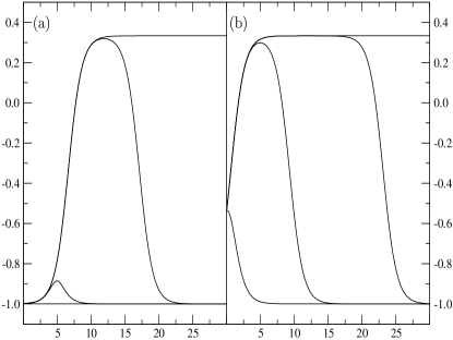
Figure 1: Evolution of the equation of state $w$ as a function of proper time $\tau/\Omega$, Eq. (86), for (a) $q_{0}=-0.001$ and (b) $q_{0}=-0.4$. The curves in both graphs correspond to values $\alpha=1,0.999999999,0.9999,0.1$ from top to bottom.

Example II:

$$x(\tau)=4\beta\ln(\Omega\tau)\,,$$ (87)

with $\Omega^{-1}\leq\tau<\infty$ and $\Omega,\beta>0\,.$ The qualitative behaviour is very similar to that of Example I. Here the brane tension has to satisfy the new condition $0<\lambda\leq\lambda_{c}$ instead of Eq. (83) in order to have $\rho>0$. The universe isotropizes in the future, with mean radius

$$a(\tau)\underset{\tau\rightarrow\infty}{\longrightarrow}(\Omega\tau)^{\beta}\,,$$ (88)

which includes radiation-domination ($\beta={1\over 2}$), matter-domination ($\beta={2\over 3}$), and power-law inflation ($\beta>1$).

Example III:

$$x(\tau)=\mathrm{arccosh}\left[\frac{(\Omega\tau)^{2\beta}+1}{(\Omega\tau)^{2\beta}-1}\right]\,,$$ (89)

with $\Omega^{-1}\leq\tau<\infty$ and $\Omega,\beta>0\,.$ The scale factors are

$$a_{i}(\tau)=\left[\frac{2(\Omega\tau)^{\beta(1-4q_{i})}}{(\Omega\tau)^{2\beta}-1}\right]^{1/4}\,,$$ (90)

so that each spatial direction can have different rates of expansion/contraction, and the universe does not isotropize in the future, unlike Examples I and II. However, the models do isotropize in the past. The mean scale factor shows that all these models are expanding in the past and collapsing in the future. (In Campos and Sopuerta (2001b) a similar qualitative behaviour was found in a Bianchi I brane when the mass of the bulk black hole is negative.) In this case the matter content never behaves as a perfect fluid.

VI Discussion

We have constructed complete (brane+bulk geometry) cosmological braneworlds with anisotropy. These solutions are the first such models with matter content. Our ansatz starts from a static form for the bulk metric, Eq. (10), with the brane moving relative to the static frame. The anisotropy arises from imposing Bianchi symmetries on a family of homogeneous 3-surfaces. For the sake of simplicity, we only considered the Abelian Bianchi I case, but other groups can be treated following the same approach.

There are two important aspects of the construction of cosmological braneworlds:

• The bulk geometry. In our case, this is given by Eq. (25), where the parameters $q_{\alpha}$ control the anisotropy. The anisotropic bulk curvature produces a nonzero Weyl anisotropic tensor ${\cal P}_{AB}$ which, as shown in the examples of the previous section, can have a fundamental impact on the dynamics. Previous studies of Bianchi brane-world dynamics which impose ad hoc assumptions on ${\cal P}_{AB}$ are unable to treat consistently the relation between the bulk and brane geometries.

• The embedding. This is where most of the freedom arises (a function of one variable). As shown by the examples in the previous section, the dynamics are very sensitive to the embedding. From the physical point of view, this leads to the question of what is the most natural state of movement for a brane. However this question cannot be answered in the phenomenological context of the RS2 scenarios.

In choosing the embedding of the brane it is very important to consider the following general feature of our models: when the brane is close to $y=y_{o}$, the effects of the anisotropy are important for the cosmological dynamics, whereas when it is located far from $y=y_{o}$, we have an effectively FRW cosmological model (in an anisotropic bulk). This fact can be seen from the relative shear eigenvalues,

$$\frac{\sigma_{i}}{\Theta}~{}\underset{x\gg 1}{\longrightarrow}~{}\frac{\ell}{9}\frac{C_{0}+3C_{i}}{u}~{}\underset{x\rightarrow\infty}{\longrightarrow}~{}0\,.$$ (91)

This is illustrated by Examples I and II, where in the future the brane isotropizes. By contrast, in Example III the brane approaches FRW in the past.

A striking feature of our models is that geometric anisotropy on the brane, from the Bianchi symmetry, imposes via the bulk curvature and the junction conditions, anisotropy on the matter content of the brane. In other words, it is not possible within our family of models to have a perfect fluid matter content (including the case of a minimally coupled scalar field) – anisotropic pressure in the matter is unavoidable unless the brane geometry reduces to Friedmann isotropy. This feature may be a consequence of the simplicity of the bulk metric ansatz that we used, but it raises an interesting challenge, i.e., to find complete Bianchi brane-world solutions with perfect fluid matter and nonzero anisotropy.

Acknowledgements:

We thank Bill Bonnor for bringing Ref. Linet (1986) to our attention. AC was supported at Portsmouth (when this work was initiated) by a university fellowship, and is supported at Heidelberg by the Alexander von Humboldt Stiftung/Foundation. RM is supported by PPARC. CFS is supported by the EPSRC and thanks the Institut für Theoretische Physik of the Universität Heidelberg for hospitality during the last stages of this work.

References

- Randall and Sundrum (1999a) L. Randall and R. Sundrum, Phys. Rev. Lett. 83, 3370 (1999a), eprint hep-ph/9905221.
- Randall and Sundrum (1999b) L. Randall and R. Sundrum, Phys. Rev. Lett. 83, 4690 (1999b), eprint hep-th/9906064.
- Horava and Witten (1996a) P. Horava and E. Witten, Nucl. Phys. B460, 506 (1996a), eprint hep-th/9510209.
- Horava and Witten (1996b) P. Horava and E. Witten, Nucl. Phys. B475, 94 (1996b), eprint hep-th/9603142.
- Binetruy et al. (2000a) P. Binetruy, C. Deffayet, and D. Langlois, Nucl. Phys. B565, 269 (2000a), eprint hep-th/9905012.
- Binetruy et al. (2000b) P. Binetruy, C. Deffayet, U. Ellwanger, and D. Langlois, Phys. Lett. B477, 285 (2000b), eprint hep-th/9910219.
- Csaki et al. (1999) C. Csaki, M. Graesser, C. F. Kolda, and J. Terning, Phys. Lett. B462, 34 (1999), eprint hep-ph/9906513.
- Cline et al. (1999) J. M. Cline, C. Grojean, and G. Servant, Phys. Rev. Lett. 83, 4245 (1999), eprint hep-ph/9906523.
- Shiromizu et al. (2000) T. Shiromizu, K.-i. Maeda, and M. Sasaki, Phys. Rev. D62, 024012 (2000), eprint gr-qc/9910076.
- Bowcock et al. (2000) P. Bowcock, C. Charmousis, and R. Gregory, Class. Quant. Grav. 17, 4745 (2000), eprint hep-th/0007177.
- Kraus (1999) P. Kraus, JHEP 12, 011 (1999), eprint hep-th/9910149.
- Ida (2000) D. Ida, JHEP 09, 014 (2000), eprint gr-qc/9912002.
- Maartens et al. (2001) R. Maartens, V. Sahni, and T. D. Saini, Phys. Rev. D63, 063509 (2001), eprint gr-qc/0011105.
- Campos and Sopuerta (2001a) A. Campos and C. F. Sopuerta, Phys. Rev. D63, 104012 (2001a), eprint hep-th/0101060.
- Campos and Sopuerta (2001b) A. Campos and C. F. Sopuerta, Phys. Rev. D64, 104011 (2001b), eprint hep-th/0105100.
- Coley (2002a) A. A. Coley, Phys. Rev. D66, 023512 (2002a), eprint hep-th/0110049.
- Coley (2002b) A. A. Coley, Class. Quant. Grav. 19, L45 (2002b), eprint hep-th/0110117.
- Hervik (2003) S. Hervik, Astrophys. Space Sci. 283, 673 (2003), eprint gr-qc/0210047.
- van den Hoogen et al. (2002) R. J. van den Hoogen, A. A. Coley, and Y. He (2002), eprint gr-qc/0212094.
- Coley and Hervik (2003) A. A. Coley and S. Hervik (2003), eprint gr-qc/0303003.
- Bruni and Dunsby (2002) M. Bruni and P. K. S. Dunsby, Phys. Rev. D66, 101301 (2002), eprint hep-th/0207189.
- Santos et al. (2001) M. G. Santos, F. Vernizzi, and P. G. Ferreira, Phys. Rev. D64, 063506 (2001), eprint hep-ph/0103112.
- Toporensky (2001) A. V. Toporensky, Class. Quant. Grav. 18, 2311 (2001), eprint gr-qc/0103093.
- Chen et al. (2001a) C.-M. Chen, T. Harko, and M. K. Mak, Phys. Rev. D64, 044013 (2001a), eprint hep-th/0103240.
- Chen et al. (2001b) C.-M. Chen, T. Harko, and M. K. Mak, Phys. Rev. D64, 124017 (2001b), eprint hep-th/0106263.
- Paul (2001) B. C. Paul, Phys. Rev. D64, 124001 (2001), eprint gr-qc/0107005.
- Barrow and Maartens (2002) J. D. Barrow and R. Maartens, Phys. Lett. B532, 153 (2002), eprint gr-qc/0108073.
- Savchenko et al. (2002) N. Y. Savchenko, S. V. Savchenko, and A. V. Toporensky, Class. Quant. Grav. 19, 4923 (2002), eprint gr-qc/0204071.
- Paul (2002) B. C. Paul, Phys. Rev. D66, 124019 (2002), eprint gr-qc/0204089.
- Harko and Mak (2003) T. Harko and M. K. Mak, Class. Quant. Grav. 20, 407 (2003), eprint gr-qc/0212075.
- van den Hoogen and Ibanez (2003) R. J. van den Hoogen and J. Ibanez, Phys. Rev. D67, 083510 (2003), eprint gr-qc/0212095.
- Aguirregabiria et al. (2003) J. M. Aguirregabiria, L. P. Chimento, and R. Lazkoz (2003), eprint gr-qc/0303096.
- Aguirregabiria and Lazkoz (2003) J. M. Aguirregabiria and R. Lazkoz (2003), eprint gr-qc/0304046.
- Frolov (2001) A. V. Frolov, Phys. Lett. B514, 213 (2001), eprint gr-qc/0102064.
- Brecher and Perry (2000) D. Brecher and M. J. Perry, Nucl. Phys. B566, 151 (2000), eprint hep-th/9908018.
- Chamblin et al. (2000) A. Chamblin, S. W. Hawking, and H. S. Reall, Phys. Rev. D61, 065007 (2000), eprint hep-th/9909205.
- Mukohyama (2000) S. Mukohyama, Phys. Lett. B473, 241 (2000), eprint hep-th/9911165.
- Vollick (2001) D. N. Vollick, Class. Quant. Grav. 18, 1 (2001), eprint hep-th/9911181.
- Cadeau and Woolgar (2001) C. Cadeau and E. Woolgar, Class. Quant. Grav. 18, 527 (2001), eprint gr-qc/0011029.
- Stephani et al. (2003) H. Stephani, D. Kramer, M. MacCallum, C. Hoenselaers, and E. Herlt, Exact solutions of Einstein’s field equations (Cambridge University Press, Cambridge, 2003).
- Linet (1986) B. Linet, J. Math. Phys. 27, 1817 (1986).
- Maartens (2000) R. Maartens, Phys. Rev. D62, 084023 (2000), eprint hep-th/0004166.
- Maartens (2001) R. Maartens (2001), eprint gr-qc/0101059.
- Barceló et al. (2003) C. Barceló, R. Maartens, C. F. Sopuerta, and F. Viniegra, Phys. Rev. D67, 064023 (2003), eprint hep-th/0211013.