Witten’s Ghost Vertex Made Simple
($bc$ and bosonized ghosts)

Abstract

First, we diagonalize the $bc$-ghost $3$-string Neumann matrices using the technique described in hep-th/0304158. Their eigenvalues are in complete agreement with the previous authors. Second, we diagonalize the $N$-string gluing vertices for the bosonized ghost system. And third, we verify the descent and associativity relations for the combined bosonic matter+ghost gluing vertices. We find that in order for these relations to be true, the vertices must be normalized by the factor $\mathcal{Z}_{N}$. Here $\mathcal{Z}_{N}$ is the partition function of the bosonic matter+ghost CFT on the gluing surface, which is the unit disc with the Neumann boundary conditions and the midpoint cone like singularity specifying by the angle excess $\pi(N-2)$.

I Introduction

Witten’s open cubic string field theory witten is usually formulated in terms of $N$-string gluing vertices GJ ; peskin2 . The expressions for these vertices in the basis which diagonalizes $L_{0}$ lead to complicated calculations. Using the fact that $K_{1}=L_{1}+L_{-1}$ commutes with Witten’s vertex, Rastelli et al. spectroscopy transformed it to the basis with $K_{1}$ diagonal. They found that the Neumann matrices in the zero momentum vertex take a simple diagonal form in this basis. Further it was realized that many calculations in the string field theory which looks complicated in the $L_{0}$-basis can be done easily and analytically in the $K_{1}$-basis. Using their technique spectroscopy the succeeding authors generalized their result to including momenta Feng:2002rm ; dima2 , ghosts dima2 ; Arefeva:2002jj ; DK2 , background $B$-field Feng:2002ib and fermions Marino:2001ny . However all of these calculation were intrinsically indirect. Recently the authors of Belov:2003df formulated a simple and direct method of changing the basis. This method is so powerful that it allowed them to diagonalize at once $N$-string Neumann matrices for all scale dimensions in the matter sector, $3$-string Neumann matrices for $\beta\gamma$ and $bc$ ghosts, and to resolve the momentum difficulty. However unlike all other cases the $3$-string $bc$-ghost’s vertex was diagonalized indirectly by relating it to the $6$-string matter Neumann matrices GJ .

The present paper has three aims. Firstly, we diagonalize the $3$-string $bc$-ghost vertex by directly changing the basis in its Neumann functions.

Secondly, we consider the general bosonized ghost system fms which is characterized by the background charge $Q$ and the parity $\varepsilon=\pm 1$. We find an expression for the $N$-string gluing vertex of this system in the $K_{1}$-basis. Then we show that ghost numbers can be added to the vertex by a unitary transformation, and discuss the differences of this construction from the one for the matter sector Belov:2003df .

Thirdly, we test the descent relations

$${}_{1\dots N,N+1}\langle V_{N+1}|V_{1}\rangle_{N+1}\stackrel{{\scriptstyle?}}{{=}}{}_{1\dots N}\,\langle V_{N}|$$ (1.1)

and other associativity relations for the combined bosonic matter+ghost gluing vertex $\langle V_{N}|$. The need to verify them arises from several inconsistencies in the calculations performed in the past two years. First, there is a strange anomaly in the multiplication of the wedge states $\langle h_{N},0|$ problem [Eq. (5.40) therein]. Second, the direct calculation of the inner product of two wedges $\langle h_{3},3|h_{3},0\rangle$ differs from the expected unity DK2 ; density . This result is in contradiction with the statement of peskin2 [Eq. (5.59) therein]. And third, assuming that the descent relation (1.1) are true for the vertices defined in GJ the authors of udi2 find some contradictions in their calculations [compare Eqs. (3.34) and (3.38) therein]. In the present paper we show that for critical bosonic string there is a finite constant $\mathcal{Z}_{N+1,1;N}$ in the rhs of the descent relation (1.1). This constant can be written as

$$\mathcal{Z}_{N+1,1;N}=\frac{\mathcal{Z}_{N}}{\mathcal{Z}_{1}\mathcal{Z}_{N+1}},$$ (1.2)

where the function $\mathcal{Z}_{N}$ is

$$\mathcal{Z}_{N}=\left[\frac{2}{N}\right]^{9/2}\,\exp\biggl{\{}\frac{27}{2}\Bigl{[}D_{0}(N)-D_{0}(2)\Bigr{]}\biggr{\}}.$$ (1.3)

The explicit expression for $D_{0}(N)$ is given in the text of this paper. Here one only needs to know that for $N\geqslant 1$ it monotonically increases, and goes to zero as $1/N$. Now it is obvious that in order to satisfy the descent relation one has to normalize the vertices by

$$\langle V_{N}|\to\mathcal{Z}_{N}\langle V_{N}|\quad\text{for}\quad N\geqslant 1.$$ (1.4)

We also verify that the normalized vertices satisfy all other associativity conditions. Notice that for $N=2$ the normalization $\mathcal{Z}_{N}$ equals 1, therefore the string inner product is not affected by (1.4). The function $\mathcal{Z}_{N}$ is nothing else but the partition function of the matter+ghost CFT on the gluing surface, which is the unit disk with Neumann boundary conditions and midpoint cone like singularity specifying by the angle excess $\pi(N-2)$.

For $N=3$ the vertex normalized as in Eq. (1.4) coincides with Witten’s original definition witten . In that paper he defined it as the Polyakov integral over the gluing surface. It seems that in most succeeding papers the Polyakov integral was changed into the correlation function on that surface, and the normalization factor $\mathcal{Z}_{N}$ was lost.

The paper is organized as follows. In Section II we review the notations used in Belov:2003df . In Section III we diagonalize the $3$-string Neumann matrices for the $bc$-ghost system. In Section IV we consider the $N$-string gluing vertices for the general bosonized ghost system. We find its representation in the $K_{1}$ basis, and describe how to change the ghost number by a unitary transformation. In Section V we prove the associativity properties of the gluing vertices for the combined bosonic matter+ghost system. In Section VI we discuss the influence of the vertex normalization (1.4) on numeric calculations in SFT. Appendix A contains necessary technical information.

II Notations

In this section we review the notations and main formulae from Belov:2003df .

Consider the primary discrete series $\mathscr{D}_{s}^{+}$ of the $SL(2,\mathbb{R})$ representations. Here $s$ is the scale dimension, $s=0,\frac{1}{2},1,\dots$. For example, $s=1$ corresponds to the zero momentum bosonic matter, $s=\frac{1}{2}$ to the fermions and $s=0$ to the bosonic matter with the zero modes. An appropriate Hilbert space $\mathcal{H}_{s}$ consists of the functions $f(z)$ analytic inside the unit disk and square-integrable on the boundary. The inner product is ruhl

$$\langle g|f\rangle=\frac{1}{\pi\Gamma(2s-1)}\,\int_{|z|\leqslant 1}\!\!d^{2}z\,\bigl{[}1-z{\overline{z}}\bigr{]}^{2s-2}\,\overline{g(z)}f(z).$$ (2.1)

The $s=\frac{1}{2}$ singularity is spurious ruhl , but there is a real one as $s$ approaches zero. The algebra $sl(2,\mathbb{R})$ is generated by $L_{0}$, $L_{\pm 1}$ which are defined by

$$L_{n}=z^{n+1}\frac{d}{dz}+(n+1)\,sz^{n}.$$ (2.2)

This representation is unitary for $s>0$.

II.1 The discrete basis

The elliptic generator $L_{0}$ has discrete eigenvalues $(m+s)$, $m=0,1,2,\dots$. Its eigenfunctions normalized by (2.1) are

$$|m,s\rangle(z)=N_{m}^{(s)}z^{m}\\ \text{with}\quad N_{m}^{(s)}=\biggl{[}\frac{\Gamma(m+2s)}{\Gamma(m+1)}\biggr{]}^{1/2}.$$ (2.3)

Notice that for $s=0$ the only singular vector is $|0,0\rangle(z)$.

II.2 The continuous basis

The generator $K_{1}=L_{1}+L_{-1}$ commutes with Witten’s star product witten , which therefore becomes simpler when it is diagonalized spectroscopy . It is convenient to map

$$z=i\tanh w,$$ (2.4)

which takes the unit disk into the strip $|\mathop{\textmd{Im}}\nolimits w|\leqslant\frac{\pi}{4}$. We assume that under a map $z\mapsto w$ the vector $f(z)$ transforms in a trivial way

$$f(z)\mapsto f(z(w)).$$ (2.4^′)

Then

$$K_{1}=-i\frac{d}{dw}+2is\tanh w.$$ (2.5)

Since this is a hyperbolic generator, its eigenvalues are all real numbers $\kappa$. The normalized eigenfunctions of (2.5) are

$$|\kappa,s\rangle(z)=\bigl{[}A_{s}(\kappa)\bigr{]}^{1/2}\,(\cosh w)^{2s}\,e^{i\kappa w},$$ (2.6)

where $A_{s}(\kappa)$ is the normalization constant:

$$A_{s}(\kappa)=\frac{2^{2s-2}}{\pi}\,\Gamma\Bigl{(}s+\frac{i\kappa}{2}\Bigr{)}\Gamma\Bigl{(}s-\frac{i\kappa}{2}\Bigr{)}.$$ (2.7)

One sees that as $s\to 0$ the function (2.7) becomes ill defined at $\kappa=0$. Nevertheless the $s=0$ $K_{1}$-eigenfunctions are well defined Belov:2003df :

$$|\kappa,0\rangle(z)=\mathscr{P}\,\frac{\sqrt{A_{1}(\kappa)}}{\kappa}\,e^{i\kappa w}\\ =\mathscr{P}\,\frac{\sqrt{A_{1}(\kappa)}}{\kappa}+|\kappa,\Omega\rangle(z).$$ (2.8)

Here $\mathscr{P}$ means the principal value, and the function $|\kappa,\Omega\rangle(z)$ can also be written as the integral of the $s=1$ $K_{1}$-eigenfunction

$$|\kappa,\Omega\rangle(z)\equiv\int_{0}^{z}d\zeta\,|\kappa,1\rangle(\zeta).$$ (2.9)

The vector $|\kappa,\Omega\rangle(z)$ is that which was found by Rastelli et al. spectroscopy . The important identity with $|\kappa,\Omega\rangle(z)$ is Belov:2003df

$$\frac{1}{2}\,\log(1+z^{2})=\int_{-\infty}^{\infty}d\kappa\,\mathscr{P}\frac{\sqrt{A_{1}(\kappa)}}{\kappa}\,|\kappa,\Omega\rangle(z).$$ (2.10a)

Differentiating this with respect to $$z$$ and using (2.9) one obtains another useful identity

$$\frac{z}{1+z^{2}}=\int_{-\infty}^{\infty}d\kappa\,\mathscr{P}\frac{\sqrt{A_{1}(\kappa)}}{\kappa}\,|\kappa,1\rangle(z).$$ (2.10b)

We will frequently use the notation $\langle\kappa,s|({\overline{z}})\equiv\overline{|\kappa,s\rangle(z)}$.

II.3 The transition matrix

The transition matrix between the discrete and continuous bases is an orthogonal matrix with elements

$$\langle m,s|\kappa,s\rangle=V_{m}^{(s)}(\kappa)\,\frac{[A_{s}(\kappa)]^{\frac{1}{2}}}{N_{m}^{(s)}}.$$ (2.11)

Here the polynomials $V_{m}^{(s)}(\kappa)$ are given by the generating function

$$(\cosh w)^{2s}\,e^{i\kappa w}=\sum_{m=0}^{\infty}V_{m}^{(s)}(\kappa)z^{m}.$$ (2.12)

Due to equation (2.9) the transition matrices for $s=0$ and $s=1$ are related as Belov:2003df

$$\langle m+1,0|\kappa,0\rangle=\langle m,1|\kappa,1\rangle\qquad(m\geqslant 0),$$ (2.13)

so $s=1$ is just $s=0$ with $m=0$ omitted.

III $3$-string Vertex for $bc$-system

III.1 Overview

The $bc$-ghost system has a background charge $Q=-3$. Due to conservation of this charge it is convenient to write a $3$-string vertex over the vacuum $\langle+|$, which is the conjugate of the ghost number $1$ vacuum $|-\rangle$ (i.e. $\langle+|-\rangle=1$). These vacua are defined by

$$b_{n}|-\rangle =0\;\,(n>-1); \quad\langle+|b_{n} =0\;\,(n<0);$$ (3.1a)

$$c_{m}|-\rangle =0\;\,(m\geqslant 1); \quad\langle+|c_{m} =0\;\,(m\leqslant 0);$$ (3.1b)

so $\{b_{0},\,b_{1},\dots\}$ and $\{c_{1},\,c_{2},\dots\}$ are the annihilation operators. The vacuum $|-\rangle$ is related to the $SL(2,\mathbb{R})$ invariant vacuum $|0\rangle$ by $|-\rangle=c(0)|0\rangle$. The $3$-string vertex over these vacua was constructed in GJ [paper II], and in our notations it reads

$$\langle V_{3}|=N_{bc}\,{}_{123}\langle+|\\ \times\exp\left[-\sum_{m=0,n=1}^{\infty}b_{m}^{(I)}\Bigl{(}\mathcal{M}^{IJ}_{bc}C\Bigr{)}_{mn}c_{n}^{(J)}\right]$$ (3.2)

Here ${}_{123}\langle+|$ means the tensor product of three Fock vacua $\langle+|$, $\bigl{(}\mathcal{M}^{IJ}_{bc}\bigr{)}_{mn}$ are the $3$-string ghost Neumann matrices and $C_{mn}=(-1)^{n}\delta_{mn}$.

To obtain an expression for the matrix elements $\bigl{(}\mathcal{M}^{IJ}_{bc}\bigr{)}_{mn}$ one can calculate the function

$$\langle V_{3}|c^{(I)}(z)b^{(J)}(z^{\prime})|-\rangle_{123}$$ (3.3)

in two different ways: using expression (3.2), and using the conformal definition of the vertex. The details of this calculation can be found, for example, in Section 4 of Bonora:2003xp or in jevicki . In our notations the result is

$$\mathcal{M}^{IJ}_{bc}(z,{\overline{z}}^{\prime})\equiv\sum_{m,n=0}^{\infty}\bigl{(}\mathcal{M}^{IJ}_{bc}\bigr{)}_{n,m+1}z^{n}{\overline{z}}^{\prime\,m}\\ =\frac{\bigl{[}h_{I}^{\prime}(z)\bigr{]}^{-1}\bigl{[}h_{J}^{\prime}(-{\overline{z}}^{\prime})\bigr{]}^{2}}{h_{I}(z)-h_{J}(-{\overline{z}}^{\prime})}\,\frac{\bigl{[}h_{I}(z)\bigr{]}^{3}-1}{\bigl{[}h_{J}(-{\overline{z}}^{\prime})\bigr{]}^{3}-1}\left[\frac{{\overline{z}}^{\prime}}{z}\right]\\ +\frac{\delta^{IJ}}{z+{\overline{z}}^{\prime}},$$ (3.4)

and $N_{bc}=\left[\frac{3\sqrt{3}}{4}\right]^{3}$. Here the maps $h_{I}(z)$ are

$$h_{I}(z) =e^{i\varphi_{I}}\left(\frac{1-iz}{1+iz}\right)^{2/3}=e^{i\varphi_{I}}\,e^{\frac{4w}{3}},$$ (3.5a)

$$h_{I}^{\prime}(z) =-\frac{4i}{3}\,\bigl{(}\cosh w\bigr{)}^{2}h_{I}(z),$$ (3.5b)

where $z=i\tanh w$, and $\varphi_{I}=\frac{2\pi}{3}(2-I)$ for $I=1,2,3$.

III.2 Diagonalizing Witten’s $3$-string ghost vertex

The aim of this section is to rewrite the operator $\mathcal{M}_{bc}^{IJ}(z,{\overline{z}}^{\prime})$ in the $K_{1}$-basis. It is known that the vertices commute with the operator $K_{1}$ GJ . So one expects that $\mathcal{M}_{bc}^{IJ}(z,{\overline{z}}^{\prime})$ takes a simple form in the $K_{1}$-basis.

To diagonalize the Neumann matrix (3.4) we first notice that the strange factors in (3.4) have very simple expression in the variable $w$

$$\frac{\bigl{[}h_{I}(z)\bigr{]}^{3}-1}{z} =-4i\,e^{2w}(\cosh w)^{2}$$ (3.6a)

and

$$\frac{\bigl{[}h_{J}(-{\overline{z}}^{\prime})\bigr{]}^{3}-1}{{\overline{z}}^{\prime}} =+4i\,e^{2{\overline{w}}^{\prime}}(\cosh{\overline{w}}^{\prime})^{2}.$$ (3.6b)

Now we proceed as in Belov:2003df — first do a binomial expansion of (3.4), then rewrite it as a contour integral, and finally do a Watson-Sommerfeld transformation. Assuming $\mathop{\textmd{Re}}\nolimits({\overline{w}}^{\prime}-w)<0$ we obtain

$$\mathcal{M}_{bc}^{IJ}(z,{\overline{z}}^{\prime})=\frac{4i}{3}\,\bigl{(}\cosh{\overline{w}}^{\prime}\bigr{)}^{2}\,(-1)^{I-J}\\ \times\oint_{C}\frac{dj}{2i\sin\pi j}\,e^{\pm i\pi j}\,\left[e^{i(\varphi_{J}-\varphi_{I})}e^{\frac{4}{3}({\overline{w}}^{\prime}-w)}\right]^{j+\frac{1}{2}}\\ +\frac{\delta^{IJ}}{z+{\overline{z}}^{\prime}}$$ (3.7)

where the contour $C$ encircles the positive real axis counterclockwise (see Figure 1). Notice that we have a sign ambiguity in the exponential, which comes from the analytic continuation of $(-1)^{j}$.

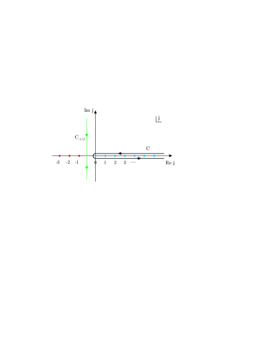
Figure 1: The dots represent the poles of the integrand in (3.7). Contour $C$ encircles the positive real axis counterclockwise. Then we deform it to the contour $C_{-\frac{1}{2}}$, which lies parallel to the imaginary axis at $\mathop{\textmd{Re}}\nolimits j=-\frac{1}{2}$.

Before deforming the contour as in Figure 1 we must worry about the convergence at infinity. Starting from here we will consider the cases $I\neq J$ and $I=J$ separately.

III.3 Matrices $\mathcal{M}_{bc}^{IJ}$ for $I\neq J$

For $I\neq J$ Eq. (3.7) can be rewritten as

$$\mathcal{M}_{bc}^{IJ}(z,{\overline{z}}^{\prime})=(\mp 1)\frac{4i}{3}\,\bigl{(}\cosh{\overline{w}}^{\prime}\bigr{)}^{2}\,(-1)^{I-J}\\ \times\oint_{C}\frac{dj}{2\sin(\pi j)}\left[e^{i(\varphi_{J}-\varphi_{I}\pm\pi)}e^{\frac{4}{3}({\overline{w}}^{\prime}-w)}\right]^{j+\frac{1}{2}}.$$ (3.8)

To deform the contour as it is shown in Figure 1 we must worry about convergence as $|\mathop{\textmd{Im}}\nolimits j|\to\infty$. To this end for $I<J$ we choose the upper “$+$” sign in the exponential. This guarantees that for $1\leqslant I<J\leqslant 3$

$$|\varphi_{J}-\varphi_{I}+\pi|\leqslant\frac{\pi}{3}.$$

Taking into account the following asymptotics as $|\mathop{\textmd{Im}}\nolimits j|\to\infty$

$$\frac{1}{\sin(\pi j)}\propto e^{-\pi|\mathop{\textmd{Im}}\nolimits j|}$$

and

$$\left|e^{\frac{4}{3}({\overline{w}}^{\prime}-w)\,j}\right|\leqslant e^{\frac{4}{3}|\mathop{\textmd{Im}}\nolimits({\overline{w}}^{\prime}-w)||\mathop{\textmd{Im}}\nolimits j|},$$

one concludes that for arbitrary small $\delta>0$ and $|\mathop{\textmd{Im}}\nolimits({\overline{w}}^{\prime}-w)|\leqslant\frac{\pi}{2}-\delta$ the integrand has at least the exponential falloff $e^{-\delta|\mathop{\textmd{Im}}\nolimits j|}$. (Oppositely, for $J<I$ one has to choose the lower “$-$” sign in the exponential. This guarantees the same falloff as $|\mathop{\textmd{Im}}\nolimits j|\to\infty$). Now we can shift the contour $C$ to $\mathop{\textmd{Re}}\nolimits j=-\frac{1}{2}$ by writing

$$j=-\frac{1}{2}-\frac{3i\kappa}{4}$$ (3.9)

to get (for $I<J$)

$$\mathcal{M}_{bc}^{IJ}(z,{\overline{z}}^{\prime})=(-1)^{I-J}\bigl{(}\cosh{\overline{w}}^{\prime}\bigr{)}^{2}\,\\ \times\int_{-\infty}^{\infty}d\kappa\,\frac{e^{\frac{\pi\kappa}{4}(2I-2J+3)}}{2\cosh\frac{3\pi\kappa}{4}}\,e^{i\kappa(w-{\overline{w}}^{\prime})}.$$ (3.10)

Notice that the integral here converges now for all $w,{\overline{w}}^{\prime}$ in the strip $|\mathop{\textmd{Im}}\nolimits w|<\frac{\pi}{4}$. Therefore (by the standard analytic continuation arguments) the right hand side represents the operator (3.4) for all $z$ and ${\overline{z}}^{\prime}$ in the unit disk.

Comparing the $\cosh$-factors in Eq. (3.10) with the ones in Eq. (2.6) one concludes that the continuum $K_{1}$-eigenfunctions correspond to $s=0$ and $s=1$. From Eqs. (2.8) and (2.6) it follows that the normalization factor of their tensor product must be $\mathscr{P}\,\frac{A_{1}(\kappa)}{\kappa}$. Insertion of unity $1=\frac{\kappa}{A_{1}(\kappa)}\,\mathscr{P}\,\frac{A_{1}(\kappa)}{\kappa}$ into Eq. (3.10) yields

$$\mathcal{M}_{bc}^{IJ}(z,{\overline{z}}^{\prime})=-\int_{-\infty}^{\infty}d\kappa\,\mu^{IJ}_{bc}(\kappa)\,|\kappa,0\rangle(z)\otimes\langle\kappa,1|({\overline{z}}^{\prime}),$$ (3.11a)

where

$$\mu^{12}_{bc}(\kappa) =+e^{+\textsl{x}}\,\frac{\sinh 2\textsl{x}}{\cosh 3\textsl{x}},$$ (3.11b)

$$\mu^{13}_{bc}(\kappa) =-e^{-\textsl{x}}\,\frac{\sinh 2\textsl{x}}{\cosh 3\textsl{x}}$$ (3.11c)

with $\textsl{x}\equiv\frac{\pi\kappa}{4}$.

III.4 Matrix $\mathcal{M}^{II}_{bc}$

For $I=J$ expression (3.4) becomes

$$\mathcal{M}_{bc}^{II}(z,{\overline{z}}^{\prime})=\frac{1}{z+{\overline{z}}^{\prime}}+\frac{4i}{3}\,\bigl{(}\cosh{\overline{w}}^{\prime}\bigr{)}^{2}\\ \times\oint_{C}\frac{dj}{2i\sin(\pi j)}\,e^{\pm i\pi j}\,\left[e^{\frac{4}{3}({\overline{w}}^{\prime}-w)}\right]^{j+\frac{1}{2}}.$$ (3.12)

This expression contains two terms, and we will consider them separately. In the second term we want to deform the contour $C$ as in Figure 1. To this end we must first worry about convergence at infinity. For general $w$ and ${\overline{w}}^{\prime}$ the integrand does not go to zero as $|\mathop{\textmd{Im}}\nolimits j|\to\infty$. However for $0<\mp\mathop{\textmd{Im}}\nolimits({\overline{w}}^{\prime}-w)\leqslant\frac{\pi}{2}$ the integrand has an exponential falloff. In this case we deform the contour $C$ as in Figure 1 by writing (3.9) to get

$$\text{second term}=\\ \pm\bigl{(}\cosh{\overline{w}}^{\prime}\bigr{)}^{2}\,\int_{-\infty}^{\infty}d\kappa\,\frac{e^{\mp\frac{3\pi\kappa}{4}}}{2\cosh\frac{3\pi\kappa}{4}}\,e^{i\kappa(w-{\overline{w}}^{\prime})}.$$

Comparing the $\cosh$-factors here with the ones in (2.6) one concludes that the continuum eigenfunctions correspond to $s=0$ and $s=1$. Therefore, we can write

$$\text{second term}=\pm\int_{-\infty}^{\infty}d\kappa\,e^{\pm\frac{3\pi\kappa}{4}}\,\frac{\sinh\frac{\pi\kappa}{2}}{\cosh\frac{3\pi\kappa}{4}}\\ \times|\kappa,0\rangle(z)\otimes\langle\kappa,1|({\overline{z}}^{\prime}),$$ (3.13)

where the eigenfunctions $|\kappa,0\rangle$ and $\langle\kappa,1|$ are defined in Eqs. (2.8) and (2.6) respectively. The representation (3.13) is valid only for $0<\mp\mathop{\textmd{Im}}\nolimits({\overline{w}}^{\prime}-w)\leqslant\frac{\pi}{2}$.

Now we need to represent the first term in Eq. (3.12) through the tensor product of $s=0$ and $s=1$ eigenfunctions. The details of this calculation can be found in Appendix A. The result is

$$\frac{1}{z+{\overline{z}}^{\prime}}=-\int_{-\infty}^{\infty}d\kappa\,e^{\pm\frac{\pi\kappa}{2}}\,|\kappa,0\rangle(z)\otimes\langle\kappa,1|({\overline{z}}^{\prime})\\ +\int_{-\infty}^{\infty}d\kappa\,\mathscr{P}\,\frac{\sqrt{A_{1}(\kappa)}}{\kappa}\otimes\langle\kappa,1|({\overline{z}}^{\prime}).$$ (3.14)

The first integral here converges for $0<\mp\mathop{\textmd{Im}}\nolimits({\overline{w}}^{\prime}-w)\leqslant\frac{\pi}{2}$, while the second integral converges for all ${\overline{z}}^{\prime}$ in the unit disk.

Substitution of Eqs. (3.13) and (3.14) into (3.12) yields

$$\mathcal{M}_{bc}^{II}(z,{\overline{z}}^{\prime})=\int_{-\infty}^{\infty}d\kappa\,\mathscr{P}\,\frac{\sqrt{A_{1}(\kappa)}}{\kappa}\otimes\langle\kappa,1|({\overline{z}}^{\prime})\\ +\int_{-\infty}^{\infty}d\kappa\,\left[\pm e^{\pm\frac{3\pi}{4}}\,\frac{\sinh\frac{\pi\kappa}{2}}{\cosh\frac{3\pi\kappa}{4}}-e^{\pm\frac{\pi\kappa}{2}}\right]\\ \times|\kappa,0\rangle(z)\otimes\langle\kappa,1|({\overline{z}}^{\prime}).$$ (3.15)

This expression has a sign ambiguity in the second term. However if we want the first integral to be convergent in the region $|\mathop{\textmd{Im}}\nolimits(w-{\overline{w}}^{\prime})|\leqslant\frac{\pi}{2}$ we must choose the upper “$+$” sign in this expression. Finally, we get

$$\mathcal{M}_{bc}^{II}(z,{\overline{z}}^{\prime})=-\int_{-\infty}^{\infty}d\kappa\,\mu_{bc}^{II}(\kappa)\,|\kappa,0\rangle(z)\otimes\langle\kappa,1|({\overline{z}}^{\prime})\\ +\int_{-\infty}^{\infty}d\kappa\,\mathscr{P}\,\frac{\sqrt{A_{1}(\kappa)}}{\kappa}\otimes\langle\kappa,1|({\overline{z}}^{\prime}),$$ (3.16a)

where

$$\mu_{bc}^{II}(\kappa)=\frac{\cosh\textsl{x}}{\cosh 3\textsl{x}}\quad\text{with}\quad\textsl{x}\equiv\frac{\pi\kappa}{4}.$$ (3.16b)

III.5 The Neumann matrices in the discrete basis

Collecting equations (3.16b) and (3.11), one concludes that the ghost $3$-string Neumann functions (3.4) have the following diagonal representation in the $K_{1}$-basis

$$\mathcal{M}_{bc}^{IJ}(z,{\overline{z}}^{\prime})=-\int_{-\infty}^{\infty}d\kappa\,\mu_{bc}^{IJ}(\kappa)\,|\kappa,0\rangle(z)\otimes\langle\kappa,1|({\overline{z}}^{\prime})\\ +\delta^{IJ}\,\int_{-\infty}^{\infty}d\kappa\,\mathscr{P}\,\frac{\sqrt{A_{1}(\kappa)}}{\kappa}\otimes\langle\kappa,1|({\overline{z}}^{\prime}),$$ (3.17a)

where $$1\leqslant I,J\leqslant 3$$,

$$\mu_{bc}^{II}(\kappa) =\frac{\cosh\textsl{x}}{\cosh 3\textsl{x}},$$ (3.17b)

$$\mu_{bc}^{I,I+1}(\kappa) =+e^{\textsl{x}}\,\frac{\sinh 2\textsl{x}}{\cosh 3\textsl{x}},$$ (3.17c)

$$\mu_{bc}^{I+1,I}(\kappa) =-e^{-\textsl{x}}\,\frac{\sinh 2\textsl{x}}{\cosh 3\textsl{x}}$$ (3.17d)

and $$\textsl{x}\equiv\frac{\pi\kappa}{4}$$.

To find the Neumann matrices $\bigl{(}\mathcal{M}_{bc}^{IJ}\bigr{)}_{n,m+1}$ we can calculate the matrix elements of the operator $\mathcal{M}_{bc}^{IJ}(z,{\overline{z}}^{\prime})$ between the vectors $\langle n,0|$ and $|m,1\rangle$. In this calculation one obviously gets a divergence for $n=0$ (see Eq. (2.3)). We can handle this divergence by considering instead of the operator $\mathcal{M}_{bc}^{IJ}(z,{\overline{z}}^{\prime})$ the vector $\mathcal{M}_{bc}^{IJ}(0,{\overline{z}}^{\prime})$ and calculate its inner product with $|m,1\rangle$. Proceeding in this way one obtains

$$\bigl{(}\mathcal{M}_{bc}^{IJ}\bigr{)}_{n+1,m+1}=-\frac{\sqrt{m+1}}{\sqrt{n+1}}\,\int_{-\infty}^{\infty}d\kappa\,\mu^{IJ}_{bc}(\kappa)\\ \times\langle n+1,0|\kappa,0\rangle\,\langle\kappa,1|m,1\rangle$$ (3.18a)

for $$n,m\geqslant 0$$ and

$$\bigl{(}\mathcal{M}_{bc}^{IJ}\bigr{)}_{0,m+1}=-\sqrt{m+1}\,\int_{-\infty}^{\infty}d\kappa\,\Bigl{[}\mu^{IJ}_{bc}(\kappa)-\delta^{IJ}\Bigr{]}\\ \times\frac{\sqrt{A_{1}(\kappa)}}{\kappa}\,\langle\kappa,1|m,1\rangle.$$ (3.18b)

Here the square roots come from calculation of the inner products of $z^{n}$ or ${\overline{z}}^{\prime m}$, appearing in the definition (3.4) of $\mathcal{M}_{bc}^{IJ}$, with the vectors $\langle n,0|$ or $|m,1\rangle$.

Taking into account Eq. (2.13) and $\mu^{IJ}_{bc}(0)=\delta^{IJ}$ we find that the representation (3.18b) and eigenvalues (3.17d) completely agree with the ones obtained in Belov:2003df [Eqs. (6.7) and (6.8) therein].

IV $N$-string Vertex for Bosonized Ghosts

IV.1 Overview

The aim of this subsection is to review a construction of LeClair et al. peskin2 of the $N$-string gluing vertex for the bosonized ghosts.

Here we consider CFT for the general bosonized ghost system fms , which is characterized by the background charge $Q$ and the parity $\varepsilon=\pm 1$. The ghost number current $j(z)=\varepsilon\partial\phi(z)$ is an anomalous primary operator of dimension $1$, and transforms under a conformal map $h(z)$ as

$$j(z)\mapsto\bigl{(}h\circ j\bigr{)}(z)=h^{\prime}(z)j(h(z))+\frac{Q}{2}\,\frac{h^{\prime\prime}(z)}{h^{\prime}(z)}.$$ (4.1)

This current has the following mode expansion

$$j(z)=\frac{j_{0}}{z}+\sum_{n=1}^{\infty}\sqrt{n}\,\Bigl{\{}a_{n}^{+}z^{n-1}-a_{n}^{-}z^{-n-1}\Bigr{\}}\\ \text{with}\quad[a_{n}^{-},\,a_{m}^{+}]=-\varepsilon\,\delta_{mn}.$$ (4.2)

Here $a^{\pm}_{m}$ are creation/annihilation operators over the vacuum $|q\rangle$, which is an eigenvector of the operator $j_{0}$ with eigenvalue $q$. Due to the anomalous transformation law (4.1) the conjugate vacuum to $|q\rangle$ is $\langle-q-Q|$. From this it follows that $j^{{\dagger}}_{0}=-j_{0}-Q$.

The OPEs of the fields $\phi(z)$ and $j(z)$ are

$$\phi(z)\phi(z^{\prime})\sim\varepsilon\log(z-z^{\prime}),$$ (4.3a)

$$j(z)\,e^{q\phi(z)}\sim\frac{q}{z-z^{\prime}}\,e^{q\phi(z^{\prime})}.$$ (4.3b)

The matter field $X^{\mu}$ can be obtained from the expression above by identifying $\varepsilon$ with $-\eta^{\mu\nu}$, $j_{0}=-i\sqrt{2\alpha^{\prime}}\,p^{\mu}$ and $a^{\pm}_{m}=\mp\frac{i}{\sqrt{m}}\,\alpha_{\mp m}^{\mu}$.

The gluing vertex for the bosonized ghosts differs in two ways from that for the $X$ field. First, it has nonzero background charge $Q$, and second the momentum eigenvalues are no longer continuous but form a discrete set. The vertex reads peskin2 [Eq. (5.1) therein]

$$\langle V_{N,\,Q}^{(0)}|=\sum_{\{q^{I}\}}\delta_{q^{1}+\dots+q^{N}+Q,0}\,\bigotimes_{I=1}^{N}{}_{I}\langle-q^{I}-Q|\,\exp\Biggl{[}\frac{\varepsilon}{2}\,\sum_{I=1}^{N}q^{I}(Q+q^{I})+\frac{\varepsilon}{2}\,\sum_{I\neq J}q^{I}N_{00}^{IJ}q^{J}\\ -\frac{\varepsilon}{2}\sum_{I=1}^{N}\sum_{n=0}^{\infty}Q\,K_{n}^{I}a_{n}^{-(I)}-\varepsilon\,\sum_{I,J=1}^{N}\sum_{n=1}^{\infty}q^{I}N_{0n}^{IJ}a_{n}^{-(J)}+\frac{\varepsilon}{2}\,\sum_{I,J=1}^{N}\sum_{m,n=1}^{\infty}a_{m}^{-(I)}N_{mn}^{IJ}a_{n}^{-(J)}\Biggr{]},$$ (4.4)

where the Neumann function coefficients $N^{IJ}_{nm}$ are defined by the same formula as the ones for the matter part of the vertex peskin2 and

$$K^{I}(z)\equiv\sum_{n=1}^{\infty}K_{n}^{I}\,\sqrt{n}\,z^{n}=\frac{h^{\prime\prime}_{I}(z)}{h_{I}^{\prime}(z)}.$$ (4.5)

The fact that the terms in the exponent contain the coefficient $Q$ is a direct consequence of the transformation law (4.1). Using the anomalous momentum conservation law and $\langle-q-Q|j_{0}=\langle-q-Q|q$ we can rewrite the exponential as peskin2

$$\exp\Biggl{[}\frac{\varepsilon}{2}\,\sum_{I,J}j_{0}^{I}\mathcal{N}_{00}^{IJ}j_{0}^{J}-\varepsilon\,\sum_{I,J}\sum_{n=1}^{\infty}j_{0}^{I}\mathcal{N}_{0n}^{IJ}a_{n}^{-(J)}+\frac{\varepsilon}{2}\,\sum_{I,J}\sum_{m,n=1}^{\infty}a_{m}^{-(I)}\mathcal{N}_{mn}^{IJ}a_{n}^{-(J)}\Biggr{]},$$ (4.6)

where the new Neumann-function coefficients are related to the old ones by

$$\mathcal{N}_{00}^{IJ} =N_{00}^{IJ}-\frac{1}{2}\,N_{00}^{II}-\frac{1}{2}\,N_{00}^{JJ},$$ (4.7a)

$$\mathcal{N}_{0m}^{IJ} =N_{0m}^{IJ}-\frac{1}{2}\,K_{m}^{J},$$ (4.7b)

$$\mathcal{N}_{mn}^{IJ} =N_{mn}^{IJ}.$$ (4.7c)

The new coefficients can be expressed in terms of the gluing maps $\{h_{I}(z)\}$ as follows peskin2

$$\mathcal{N}_{00}^{IJ} =\bigl{(}1-\delta^{IJ}\bigr{)}\,\log\Biggl{[}\frac{|h_{I}(0)-h_{J}(0)|}{|h^{\prime}_{I}(0)h^{\prime}_{J}(0)|^{\frac{1}{2}}}\Biggr{]},$$ (4.8a)

$$\mathcal{N}^{IJ}_{0}(z) \equiv\sum_{n=1}^{\infty}\mathcal{N}_{0n}^{IJ}\,\sqrt{n}\,z^{n-1}$$

$$=- \frac{h^{\prime}_{J}(z)}{h_{I}(0)-h_{J}(z)}-\frac{\delta^{IJ}}{z}-\frac{h_{J}^{\prime\prime}(z)}{2h_{J}^{\prime}(z)},$$ (4.8b)

$$\mathcal{N}^{IJ}(z,z^{\prime}) \equiv\sum_{m,n=1}^{\infty}\mathcal{N}_{mn}^{IJ}\sqrt{mn}\,z^{m-1}\,z^{\prime\,n-1}$$

$$= \frac{h^{\prime}_{I}(z)h^{\prime}_{J}(z^{\prime})}{\bigl{[}h_{I}(z)-h_{J}(z^{\prime})\bigr{]}^{2}}-\frac{\delta^{IJ}}{(z-z^{\prime})^{2}}.$$ (4.8c)

Notice that all functions here are manifestly $PSL(2)$ invariant peskin2 [pp. 487–488], i.e. they do not change under $\{h_{I}\}\to\{T\circ h_{I}\}$ with $T(z)\in PSL(2)$. Therefore all Neumann coefficients $\mathcal{N}_{mn}$ are $SL(2,\mathbb{R})$ invariant. Let us remember that, for example, the generating function for the coefficients $N_{0n}^{IJ}$ does depend on a choice of the $SL(2,\mathbb{R})$ frame. However this dependence is cancelled by the nonanomalous momentum conservation, and therefore the $X$ vertex is $SL(2)$ invariant.

Writing the vertex in the form (4.6) eliminates the explicit dependence on the background charge $Q$. In this notation the $X^{\mu}$ vertex can be obtained simply by changing $\varepsilon$ to $-\eta^{\mu\nu}$, $j_{0}=-i\sqrt{2\alpha^{\prime}}p^{\mu}\,$ and $a^{\pm}_{n}\to\mp i\,\frac{\alpha_{\mp_{n}}^{\mu}}{\sqrt{n}}$. Of course some of the terms in Eq. (4.8b) will drop out due to the normal (nonanomalous) momentum conservation peskin2 .

For Witten’s $N$-string vertex the maps $h_{I}(z)$ are

$$h_{I}(z) =\left(\frac{1-iz}{1+iz}\right)^{2/N}=e^{i\varphi_{I}}e^{4w/N},$$ (4.9a)

$$h_{I}^{\prime}(z) =-\frac{4i}{N}\,\bigl{(}\cosh w\bigr{)}^{2}h_{I}(z),$$ (4.9b)

where $z=i\tanh w$ and $\varphi_{I}=\frac{2\pi}{N}(\alpha_{N}-I)$. Here $\alpha_{N}$ is a real number which is chosen in such a way that all angles $\varphi_{I}$ lie in the range $(-\pi,\pi]$.

IV.2 Diagonalization of the Neumann Coefficients

IV.2.1 Operator $\mathcal{N}^{IJ}$

The operator $\mathcal{N}^{IJ}(z,z^{\prime})$ was diagonalized in Section III of Belov:2003df :

$$\mathcal{N}^{IJ}(z,-{\overline{z}}^{\prime})=\int_{-\infty}^{\infty}d\kappa\,\mu_{1,N}^{IJ}(\kappa)\\ \times|\kappa,1\rangle(z)\otimes\langle\kappa,1|({\overline{z}}^{\prime}),$$ (4.10)

where $|\kappa,1\rangle(z)$ is defined in (2.6), $\langle\kappa,1|({\overline{z}}^{\prime})\equiv\overline{|\kappa,1\rangle(z^{\prime})}\;$ and

$$\mu_{1,N}^{II}(\kappa) =-\frac{\sinh(N-2)\textsl{x}}{\sinh N\textsl{x}},$$ (4.11a)

$$\mu_{1,N}^{IJ}(\kappa) =e^{+\textsl{x}(N+2I-2J)}\,\frac{\sinh 2\textsl{x}}{\sinh N\textsl{x}}\quad(I<J),$$ (4.11b)

$$\mu_{1,N}^{IJ}(\kappa) =e^{-\textsl{x}(N-2I+2J)}\,\frac{\sinh 2\textsl{x}}{\sinh N\textsl{x}}\quad(I>J).$$ (4.11c)

Here $\textsl{x}\equiv\frac{\pi\kappa}{4}$.

IV.2.2 Matrix $\mathcal{N}^{IJ}_{00}$

Substitution of the maps (4.9) into (4.8a) yields

$$\mathcal{N}_{00}^{IJ}=(1-\delta^{IJ})\,\log\left[\frac{N}{2}\,\sin\left(\frac{\pi}{N}\,|I-J|\right)\right].$$ (4.12)

This expression coincides with the matrix $M^{\prime\,IJ}_{N,\,00}$ which is defined by equation (5.8) in Belov:2003df . The numbers $\mathcal{N}_{00}^{IJ}$ can also be represented by the following integral

$$\mathcal{N}_{00}^{IJ}=-\int_{-\infty}^{\infty}d\kappa\,\frac{A_{1}(\kappa)}{\kappa^{2}}\,\biggl{\{}\frac{1}{2}\,\Bigl{[}\mu^{IJ}_{1,N}(\kappa)+\mu^{JI}_{1,N}(\kappa)\Bigr{]}\\ -\mu^{II}_{1,N}(\kappa)+\delta^{IJ}-1\biggr{\}}.$$ (4.13)

The simplest way to obtain this expression is to notice that it can also be written as the following limit

$$-\lim_{s\to+0}\int_{-\infty}^{\infty}d\kappa\,A_{s}(\kappa)\,\biggl{\{}\frac{1}{2}\,\Bigl{[}\mu^{IJ}_{s,N}(\kappa)+\mu^{JI}_{s,N}(\kappa)\Bigr{]}\\ -\mu^{II}_{s,N}(\kappa)+\delta^{IJ}-1\biggr{\}},$$

which was calculated in Eqs. (5.7) – (5.9) in Belov:2003df with the result $M^{\prime\,IJ}_{N,\,00}$.

IV.2.3 Vector $\mathcal{N}_{0}^{IJ}$

Substitution of the maps (4.9) into (4.8b) yields

$$\mathcal{N}_{0}^{IJ}(-{\overline{z}}^{\prime})=\frac{4i}{N}\,\bigl{(}\cosh{\overline{w}}^{\prime}\bigr{)}^{2}\,\frac{e^{i(\varphi_{J}-\varphi_{I})}e^{4{\overline{w}}^{\prime}\!/N}}{1-e^{i(\varphi_{J}-\varphi_{I})}e^{4{\overline{w}}^{\prime}\!/N}}\\ +\frac{\delta^{IJ}}{{\overline{z}}^{\prime}}-\frac{{\overline{z}}^{\prime}}{1+{\overline{z}}^{\prime\,2}}+\frac{2i}{N}\,\bigl{(}\cosh{\overline{w}}^{\prime}\bigr{)}^{2}.$$ (4.14)

Assuming $\mathop{\textmd{Re}}\nolimits{\overline{w}}^{\prime}<0$ we can expand the first term in a binomial series, and then rewrite it as a contour integral. All other terms we leave as they are for a while. So the first term becomes

$$\text{first term}=-\frac{4i}{N}\,\bigl{(}\cosh{\overline{w}}^{\prime}\bigr{)}^{2}\,\oint_{C}\frac{dj}{2i\sin(\pi j)}\,\\ \times e^{i(\varphi_{J}-\varphi_{I}\pm\pi)(j+1)}e^{\frac{4{\overline{w}}^{\prime}}{N}(j+1)},$$ (4.15)

where the contour $C$ encircles the positive real axis in the counterclockwise direction (see Figure 2). Notice the sign ambiguity in the exponential, which comes from the analytic continuation of $(-1)^{j}$.

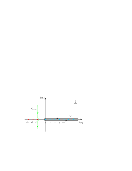
Figure 2: The dots represent the poles of the integrand in (4.15). Contour $C$ encircles the positive real axis counterclockwise. Then we deform it to the contour $C_{-1+0}$, which lies parallel to the imaginary axis at $\mathop{\textmd{Re}}\nolimits j=-1$ and passes the pole at $j=-1$ on the right.

Now we are going to deform the contour $C$ to lie parallel to the imaginary axis as in Figure 2. To this end we need to worry about the convergence as $|\mathop{\textmd{Im}}\nolimits j|\to\infty$. Let us assume $I\leqslant J$. In this case the integral will have the exponential falloff if we choose the upper “$+$” sign and temporary assume $0<-\mathop{\textmd{Im}}\nolimits{\overline{w}}^{\prime}<\frac{\pi}{4}$. With these assumptions we can safely deform the contour $C$ as in Figure 2 by writing

$$j=-1+0-\frac{iN\kappa}{4}$$

to get

$$\text{first term}=\bigl{(}\cosh{\overline{w}}^{\prime}\bigr{)}^{2}\int_{-\infty}^{\infty}\frac{d\kappa}{2\sinh\bigl{(}\frac{\pi N\kappa}{4}+i0\bigr{)}}\,\\ \times e^{\frac{\pi\kappa}{4}(N+2I-2J)}\,e^{-i\kappa{\overline{w}}^{\prime}}.$$ (4.16)

Using the fact that

$$\frac{1}{\sinh\bigl{(}\frac{\pi N\kappa}{4}+i0\bigr{)}}=\mathscr{P}\frac{1}{\sinh\frac{\pi N\kappa}{4}}-\frac{4i}{N}\,\delta(\kappa)$$

one finds that the term in Eq. (4.16) coming from the $\delta$-function cancels the last term in Eq. (4.14). Now we represent $1/{\overline{z}}^{\prime}$ in Eq. (4.14) as in Eq. (3.14) with the “$+$” sign, and write ${\overline{z}}^{\prime}/(1+{\overline{z}}^{\prime\,2})$ as in Eq. (2.10b) to get

$$\mathcal{N}_{0}^{IJ}(-{\overline{z}}^{\prime})=\int_{-\infty}^{\infty}d\kappa\,\mathscr{P}\frac{\sqrt{A_{1}(\kappa)}}{\kappa}\,\\ \times\Bigl{(}\mu_{1,N}^{IJ}(\kappa)-1+\delta^{IJ}\Bigr{)}\,\langle\kappa,1|({\overline{z}}^{\prime}),$$ (4.17)

where $\mu_{1,N}^{IJ}(\kappa)$ is defined in (4.11). Notice now that the integral in the rhs converges for all ${\overline{w}}^{\prime}$ in the strip $|\mathop{\textmd{Im}}\nolimits{\overline{w}}^{\prime}|<\frac{\pi}{4}$. Therefore (by the standard analytic continuation arguments) this expression represents the vector $\mathcal{N}_{0}^{IJ}(z)$ for all $z$ in the unit disk. One can easily check that equation (4.17) remains the same if we assume $I\geqslant J$ and choose the “$-$” sign in Eqs. (4.14) and (3.14).

IV.3 The $N$-string Vertex in the Continuous Basis

IV.3.1 Vertex in the continuous basis

We introduce the $s=1$ continuum oscillators

$$a^{\pm}(\kappa)=\sum_{n=0}^{\infty}a^{\pm}_{n+1}\,\langle\kappa,1|n,1\rangle\\ \text{with}\quad[a^{-}(\kappa),\,a^{+}(\kappa^{\prime})]=-\varepsilon\delta(\kappa-\kappa^{\prime}).$$ (4.18)

In order to write the vertex we also need a twist operator $C$, which roughly speaking corresponds to the substitution ${\overline{z}}^{\prime}\to-{\overline{z}}^{\prime}$. It is defined GJ in the discrete basis by $(Ca^{\pm})_{n}=(-1)^{n}a^{\pm}_{n}$. Hence in the continuous basis it becomes

$$\bigl{(}Ca^{\pm}\bigr{)}(\kappa)=-a^{\pm}(-\kappa).$$ (4.19)

Finally, substituting Eqs. (4.10), (4.17) into (4.6) and using (4.18) one obtains

$$\langle V_{N,\,Q}^{(0)}|=\sum_{\{q^{I}\}}\bigotimes_{I=1}^{N}\,{}_{I}\langle-q^{I}-Q|\,\delta_{j^{1}_{0}+\dots+j^{N}_{0}+Q,0}\,\exp\Biggl{[}-\frac{\varepsilon}{2}\sum_{I,J=1}^{N}\,\int_{-\infty}^{\infty}d\kappa\,a^{-(I)}(\kappa)\,\mu^{IJ}_{1,N}(\kappa)\,\bigl{(}Ca^{-(J)}\bigr{)}(\kappa)\\ +\varepsilon\sum_{I,J=1}^{N}j_{0}^{I}\int_{-\infty}^{\infty}d\kappa\,\mathscr{P}\frac{\sqrt{A_{1}(\kappa)}}{\kappa}\,\Bigl{\{}\mu^{IJ}_{1,N}(\kappa)-1+\delta^{IJ}\Bigr{\}}\bigl{(}Ca^{-(J)}\bigr{)}(\kappa)+\frac{\varepsilon}{2}\sum_{I,J=1}^{N}\,j_{0}^{I}\mathcal{N}^{IJ}_{00}j_{0}^{J}\Biggr{]},$$ (4.20)

where $j_{0}$ is the ghost number operator, $\langle-q-Q|j_{0}=q\langle-q-Q|$, the continuous oscillators $a^{-}(\kappa)$ are defined in (4.18), the $N$-string Neumann matrix eigenvalues $\mu_{1,N}^{IJ}$ are defined in (4.11), and the coefficients $\mathcal{N}^{IJ}_{00}$ are listed in (4.12). Notice that the gluing vertex for the matter field $X^{\mu}$ can be obtained from this by putting $Q=0$ and replacing $\varepsilon$ with $-\eta^{\mu\nu}$, $j_{0}=-i\sqrt{2\alpha^{\prime}}p_{\mu}$ and $a^{-(I)}\to a^{-(I)}_{\mu}$ (compare (4.20) with Eq. (5.12) from Belov:2003df ).

IV.3.2 The unitary transformation

In Belov:2003df it was shown that the $s=0$ $N$-string matter vertex can be obtained from the zero momentum (i.e. $s=1$) vertex by the unitary transformation

$$U_{p}=\exp\biggl{\{}i\sqrt{2\alpha^{\prime}}\,\hat{p}\int_{-\infty}^{\infty}d\kappa\,\mathscr{P}\frac{\sqrt{A_{1}(\kappa)}}{\kappa}\\ \times\Bigl{[}a^{+}(\kappa)+a^{-}(\kappa)\Bigr{]}\biggr{\}}.$$ (4.21)

In the case of nonzero background charge $Q$ the appropriate unitary operator is

$$U_{j_{0}}=\exp\biggl{\{}\varepsilon\Bigl{(}j_{0}+\frac{Q}{2}\Bigr{)}\int_{-\infty}^{\infty}d\kappa\,\mathscr{P}\frac{\sqrt{A_{1}(\kappa)}}{\kappa}\\ \times\Bigl{[}a^{+}(\kappa)+a^{-}(\kappa)\Bigr{]}\biggr{\}}.$$ (4.22)

Here the linear combination of $j_{0}$ and $Q$ was fixed from the conjugation property fms of $j_{0}$: $j_{0}^{{\dagger}}=-j_{0}-Q$. Notice that in contrast to (4.21) the unitary transformation (4.22) remains non-trivial even for $j_{0}=0$. Under this unitary transformation the $s=1$ continuum oscillator $a^{\pm}(\kappa)$ transforms to the $s=0$ oscillator

$$a^{\pm}(\kappa,j_{0})\equiv U^{-1}_{j_{0}}a^{\pm}(\kappa)U_{j_{0}}\\ =\pm\Bigl{(}j_{0}+\frac{Q}{2}\Bigr{)}\,\mathscr{P}\frac{\sqrt{A_{1}(\kappa)}}{\kappa}+a^{\pm}(\kappa).$$ (4.23)

Now let us try to proceed as in Belov:2003df and add the ghost numbers by applying $N$ copies of the unitary transformation (4.22). To this end we have to regularize the principal value in (4.22). It does not matter what regularization we choose, the final result should be regularization independent. For definite we will assume the following regularization Belov:2003df

$$U_{j_{0},s}=\exp\biggl{\{}\varepsilon\Bigl{(}j_{0}+\frac{Q}{2}\Bigr{)}\,\int_{-\infty}^{\infty}d\kappa\,\xi_{s}(\kappa)\\ \times\Bigl{[}a^{+}(\kappa)+a^{-}(\kappa)\Bigr{]}\biggr{\}},$$ (4.24)

where

$$\xi_{s}(\kappa)=\sqrt{A_{s}(\kappa)}=\frac{\mathop{\mathrm{sgn}}\nolimits(\kappa)}{\sqrt{\kappa^{2}+4s^{2}}}\,\sqrt{A_{1+s}(\kappa)}.$$ (4.25)

Now $U_{j_{0}}$ can be normal ordered

$$U_{j_{0},s}=\exp\left\{-\frac{\varepsilon}{2}\Bigl{(}j_{0}+\frac{Q}{2}\Bigr{)}^{2}\,\langle\xi_{s},\xi_{s}\rangle\right\}\,:U_{j_{0},s}\!:,$$ (4.26)

where

$$\langle\xi_{s},\xi_{s}\rangle=\int_{-\infty}^{\infty}d\kappa\,A_{s}(\kappa)=\Gamma(2s).$$

Whenever possible we will write $\langle\xi_{s},\xi_{s}\rangle$ instead of its value $\Gamma(2s)$. We will do this in order to be able to choose another regularization without extra problems.

So we want to calculate

$$\lim_{s\to+0}\langle V^{(1)}_{N}|\bigotimes_{I=1}^{N}U_{j_{0}^{I},s}\,\delta_{j_{0}^{1}+\dots+j_{0}^{N}+Q,0},$$ (4.27)

where the vertex $\langle V^{(1)}_{N}|$ is defined by the first line in (4.20). Substitution of Eq. (4.26) yields

$$\lim_{s\to+0}\sum_{q^{1},\dots,q^{N}}\bigotimes_{I=1}^{N}{}_{I}\langle-q^{I}-Q|\,\delta_{q^{1}+\dots+q^{N}+Q,0}\exp\biggl{\{}-\frac{\varepsilon}{2}\,\sum_{I,J=1}^{N}\int_{-\infty}^{\infty}d\kappa\,a^{-(I)}(\kappa)\,\mu^{IJ}_{1,N}(\kappa)\bigl{(}Ca^{-(J)}\bigr{)}(\kappa)\\ +\varepsilon\sum_{I,J=1}^{N}\Bigl{(}q^{I}+\frac{Q}{2}\Bigr{)}\int_{-\infty}^{\infty}d\kappa\,\xi_{s}(\kappa)\,\Bigl{[}\mu^{IJ}_{1,N}(\kappa)+\delta^{IJ}\Bigr{]}\bigl{(}Ca^{-(J)}\bigr{)}(\kappa)\\ -\frac{\varepsilon}{2}\sum_{I,J=1}^{N}\Bigl{(}q^{I}+\frac{Q}{2}\Bigr{)}\Bigl{(}q^{J}+\frac{Q}{2}\Bigr{)}\int_{-\infty}^{\infty}d\kappa\,\xi_{s}(\kappa)\Bigl{[}\mu^{IJ}_{1,N}(\kappa)+\delta^{IJ}\Bigr{]}\xi_{s}(\kappa)\biggr{\}}$$

One sees that the integrals in the first and second term in the exponential are well defined as $s\to 0$, but there is a problem with the $s\to 0$ limit in the third term. In the second term we can substitute $Q=-\sum_{I}q^{I}$ and use that $\sum_{I}[\mu^{IJ}(\kappa)+\delta^{IJ}]=2$ to obtain

$$\text{second term}=\varepsilon\sum_{I,J=1}^{N}q^{I}\int_{-\infty}^{\infty}d\kappa\,\mathscr{P}\frac{\sqrt{A_{1}(\kappa)}}{\kappa}\\ \times\Bigl{[}\mu^{IJ}_{1,N}(\kappa)+\delta^{IJ}-1\Bigr{]}\bigl{(}Ca^{-(J)}\bigr{)}(\kappa).$$

In the third term, we can use equation (4.13) and the anomalous conservation law to get

$$\text{third term}=\frac{\varepsilon}{2}\sum_{I,J=1}^{N}q^{I}\mathcal{N}_{00}^{IJ}q^{J}\\ -\frac{\varepsilon\,Q^{2}}{2}\,\int_{-\infty}^{\infty}d\kappa\,\frac{A_{1}(\kappa)}{\kappa^{2}}\,\Bigl{[}\mu^{II}_{1,N}(\kappa)-\mu_{1,N}^{II}(0)\Bigr{]}\\ -\frac{\varepsilon\,Q^{2}}{2}\,\frac{(N-2)^{2}}{2N}\,\langle\xi_{s},\xi_{s}\rangle.$$

The integral here is easy to calculate, and we finally get the relation

$$\langle V_{N,Q}^{(0)}|\{q^{I}\}\rangle=\lim_{s\to+0}e^{F_{N,s}}\,\langle V_{N,Q}^{(1)}|\\ \times U_{q^{1}}\otimes\dots\otimes U_{q^{N}}\,\delta_{q^{1}+\dots+q^{N}+Q,0}\,,$$ (4.28)

where

$$F_{N,s}\equiv\frac{\varepsilon\,Q^{2}}{2}\,\frac{(N-2)^{2}}{2N}\,\langle\xi_{s},\xi_{s}\rangle\\ +\frac{\varepsilon\,Q^{2}}{2}\,\Bigl{[}\log\frac{N}{2}-\frac{N-2}{N}\,\log 2\Bigr{]}.$$ (4.29)

Notice that for general $Q$ the function $F_{N,s}$ is zero only for $N=2$. This means that the string inner product $\langle V_{2}^{(0)}|$ is not affected by this singularity. For $Q=0$ $F_{N,s}$ is identically zero, and hence after replacing $q^{I}\to-i\sqrt{2\alpha^{\prime}}p^{I}_{\mu}$ equation (4.28) reproduces the result of Belov:2003df for the matter sector.

V Associativity of Witten’s Star Product

V.1 Descent Relation between the Gluing Vertices

The aim of this section is to verify the following descent relation:

$${}_{1\dots N}\langle V_{N}|={}_{1\dots N,N+1}\langle V_{N+1}|V_{1}\rangle_{N+1},$$ (5.1)

where $\langle V_{N}|$ is the combined matter+ghost gluing $N$-string vertex. The combined vertex $\langle V_{N}|$ has the form (4.20) with the replacements: $a^{-}\to a^{-}_{\mu}$ ($\mu=-1,\dots,D-1$) where $\mu=-1$ corresponds to the ghost oscillator and $\mu=0,\dots,D-1$ to the matter ones; $\varepsilon\to-\eta^{\mu\nu}$ where $\eta^{\mu\nu}=\mathrm{diag}(-\varepsilon,-1,1,\dots,1)$; and $j_{0}\to j_{0}^{\mu}=(j_{0},-i\sqrt{2\alpha^{\prime}}\vec{p}\,)$.

We know that the vertex depending on the momenta and ghost numbers can be obtained from the $s=1$ vertex by the unitary transformation as in (4.28). Since adding the momentum does not produce any divergencies Belov:2003df we put it equal to zero. So we need to calculate the following product

$$e^{F_{N+1,s}+F_{1,s}}\,{}_{1\dots N,N+1}\langle V_{N+1}^{(1)}|V_{1}^{(1)}\rangle_{N+1}\\ \times U_{q^{1}}\otimes\dots\otimes U_{q^{N}}\,\delta_{q^{1}+\dots+q^{N}+Q,0}.$$ (5.2)

The inner product in the $(N+1)^{\text{th}}$ tensor component is easy to calculate:

$${}_{1\dots N,N+1}\langle V_{N+1}^{(1)}|V_{1}^{(1)}\rangle_{N+1}=\det\bigl{(}1-\mu_{N+1}^{11}\bigr{)}^{-\frac{D+1}{2}}\,\\ \times{}_{1\dots N}\langle 0|\exp\left[\frac{1}{2}\,\sum_{\mu,\nu=-1}^{D-1}\sum_{I,J=1}^{N}\,\int_{-\infty}^{\infty}d\kappa\,a^{-(I)}_{\mu}(\kappa)\,\eta^{\mu\nu}\left\{\mu_{N+1}^{IJ}+\frac{\mu_{N+1}^{I,N+1}\mu_{N+1}^{N+1,J}}{1-\mu_{N+1}^{11}}\right\}(\kappa)\,\bigl{(}Ca^{-(J)}_{\nu}\bigr{)}(\kappa)\right],$$

where $\mu_{N}^{IJ}\equiv\mu_{1,N}^{IJ}$. It is a matter of simple algebra to show that the term in $\{\}$ equals $\mu^{IJ}_{N}(\kappa)$. Hence we see that the descent relation is actually satisfied up to a numeric coefficient

$${}_{1\dots N,N+1}\langle V_{N+1}|V_{1}\rangle_{N+1}=(\mathcal{Z}_{N+1,1;N})\,{}_{1\dots N}\,\langle V_{N}|,$$ (5.3)

where

$$\log\mathcal{Z}_{N+1,1;N}\equiv-\frac{D+1}{2}\,\log\det\bigl{(}1-\mu_{N+1}^{11}\bigr{)}\\ +F_{N+1,s}+F_{1,s}-F_{N,s}$$ (5.4)

and $F_{N,s}$ is defined in (4.29). In other words $\log\mathcal{Z}_{N+1,1;N}$ is

$$\log\mathcal{Z}_{N+1,1;N}\equiv+\frac{\varepsilon Q^{2}}{2}\,\log\frac{N+1}{2N}\\ -\frac{D+1}{2}\int_{-\infty}^{\infty}d\kappa\,\log\bigl{(}1-\mu_{N+1}^{11}(\kappa)\bigr{)}\,\rho_{1}(\kappa)\\ +\frac{\varepsilon Q^{2}}{2}\,\frac{(N-1)(N+2)}{N(N+1)}\,\Bigl{\{}\langle\xi_{s},\xi_{s}\rangle+\log 2\Bigr{\}},$$ (5.5)

where $\rho_{1}(\kappa)$ is the trace density which was calculated in density

$$\rho_{1}(\kappa)=\frac{1}{\pi}\,\Bigl{[}\langle\xi_{s},\xi_{s}\rangle+\log 2\Bigr{]}\\ -\frac{1}{4\pi}\biggl{[}\psi\Bigl{(}1+\frac{i\kappa}{2}\Bigr{)}+\psi\Bigl{(}1-\frac{i\kappa}{2}\Bigr{)}+2\gamma_{E}\biggr{]}.$$

From this it follows that $\mathcal{Z}_{2,1;1}=1$. If the descent relation (5.1) were true, all $\mathcal{Z}_{N+1,1;N}$ with $N>1$ would be $1$. But as we will see in a moment $\mathcal{Z}_{N+1,1;N}$ is a nontrivial function of $N$, and therefore the vertices must contain an additional normalization factor.

For the critical bosonic string ($D=26$, $\varepsilon=1$ and $Q=-3$) $\mathcal{Z}_{N+1,1;N}$ is a finite function of $N$

$$\log\mathcal{Z}_{N+1,1;N}=-\frac{9}{2}\,\sum_{\alpha\in A}s_{\alpha}\log\alpha\\ +\frac{27}{2}\,\sum_{\alpha\in A}s_{\alpha}D_{0}(\alpha),$$ (5.6)

where $A=\{2,N,N+1,1\}$, $\{s_{\alpha}|\alpha\in A\}=\{1,1,-1,-1\}$ and

$$D_{0}(\alpha)=\int_{0}^{\infty}\frac{dt}{t}\,\left\{\frac{\coth\frac{t}{\alpha}-\frac{\alpha}{t}}{e^{t}-1}-\frac{1}{3\alpha}\,\frac{1}{1+t}\right\}.$$ (5.7)

The details of this calculation will be presented in BG . From the representation (5.6) it follows that $\mathcal{Z}_{N+1,1;N}$ can be written as

$$\mathcal{Z}_{N+1,1;N}=\frac{\mathcal{Z}_{N}}{\mathcal{Z}_{1}\mathcal{Z}_{N+1}}.$$ (5.8)

Here the logarithm of $\mathcal{Z}_{N}$ is given by

$$\log\mathcal{Z}_{N}=-\frac{9}{2}\,\log\frac{N}{2}+\frac{27}{2}\,\Bigl{[}D_{0}(N)-D_{0}(2)\Bigr{]}.$$ (5.9)

Notice that the function $\mathcal{Z}_{N}$ can not be uniquely determined from the relation (5.8). It is defined up to a rescaling

$$\mathcal{Z}_{N}\mapsto(\text{const})^{N-2}\mathcal{Z}_{N}.$$ (5.10)

The function $\mathcal{Z}_{N}$ defined in (5.9) monotonically goes to zero on the interval $[1,\infty)$, and its asymptotic at infinity is

$$\mathcal{Z}_{N}\propto\left[\frac{2}{N}\right]^{9/2}\,\exp\biggl{\{}-\frac{27}{2}D_{0}(2)+O\Bigl{(}\frac{1}{N}\Bigr{)}\biggr{\}}.$$

Now it is obvious that in order to have the descent relation (5.1) one has to introduce the normalized gluing vertices $\langle\!\langle V_{N}|$, which are defined by

$$\langle\!\langle V_{N}|=\mathcal{Z}_{N}\,\langle V_{N}|\quad\text{for}\quad N\geqslant 1.$$ (5.11)

The normalization $\mathcal{Z}_{N}$ is given by (5.9) or any of (5.10). Notice that $\mathcal{Z}_{2}=1$ independently on the choice of the scaling factor in (5.10). The ambiguity (5.10) is closely related to the string field redefinition. Indeed the factor $(\text{const})^{N-2}$ in the vertex can be cancelled by simultaneous rescaling of the string field $\mathcal{A}\mapsto(\text{const})^{-1}\mathcal{A}$ and the coupling constant $g_{o}\mapsto(\text{const})^{-1}g_{o}$. The natural choice of the factor in (5.10) is that where $\mathcal{Z}_{N}$ coincides with the partition function of the bosonic matter+ghost CFT on the gluing surface, which is the unit disk with Neumann boundary conditions and the angle excess $\pi(N-2)$. This choice is basically follows from the relation

$$\mathcal{Z}_{N}=\langle\!\langle V_{N}|\bigl{(}|0\rangle_{1}\otimes\dots\otimes|0\rangle_{N}\bigr{)},$$

where $\langle\!\langle V_{N}|$ is supposed to be a surface (multi)state, and therefore the rhs must be the partition function of this surface [see Figure 5 in zwiebach ].

For $N=3$ the normalized as in Eq. (5.11) $3$-string vertex coincides with Witten’s original definition witten . In that paper he defined it as the Polyakov integral over the gluing surface which, of course, includes the partition function in its definition.

Notice that in Moyal formulation of SFT (MSFT) Bars:2002nu the star product is associative by construction and there is a way to obtain the Neumann matrix elements from it Bars:2002nu . Therefore it should be also possible to extract the normalization of the gluing vertices and compare them with $\mathcal{Z}_{N}$.

V.2 Associativity

The associativity requires many relations between the gluing vertices. For example,

$$\Bigl{(}{}_{123}\langle V_{3}|\otimes{}_{456}\langle V_{3}|\Bigr{)}|V_{2}\rangle_{34}={}_{1256}\langle V_{4}|,\\ \Bigl{(}{}_{123}\langle V_{3}|\otimes{}_{456}\langle V_{3}|\otimes{}_{78}\langle V_{2}|\Bigr{)}|V_{3}\rangle_{368}={}_{12457}\langle V_{5}|$$ (5.12)

and many many more. The question is if these relations are satisfied for the normalized vertices (5.11). Actually the question is only about the normalization factors, since the exponentials were worked out in peskin2 ; Furuuchi:2001df .

We claim that the normalized vertices (5.11) indeed satisfy the relations like (5.12). The proof is simple and does not require complicated calculations. Let us prove, for example, the first relation in (5.12). Suppose that it is false, and there is a constant $A\neq 1$ in the rhs:

$$\Bigl{(}{}_{123}\langle\!\langle V_{3}|\otimes{}_{456}\langle\!\langle V_{3}|\Bigr{)}|V_{2}\rangle\!\rangle_{34}=A\;{}_{1256}\langle\!\langle V_{4}|.$$

Now we contract this equation with the identity state $|V_{1}\rangle\!\rangle{}_{6}$ in the $6$-th tensorial space. Using the descent relations (5.1) we obtain

$$\Bigl{(}{}_{123}\langle\!\langle V_{3}|\otimes{}_{45}\langle\!\langle V_{2}|\Bigr{)}|V_{2}\rangle\!\rangle_{34}=A\;{}_{125}\langle\!\langle V_{3}|.$$

Noticing that ${}_{45}\langle\!\langle V_{2}|V_{2}\rangle\!\rangle_{34}=\delta_{53}$ one finds that the constant $A$ equals $1$. So the first relation in (5.12) is true. Actually all relations like (5.12) can be proved in this manner. Therefore the normalized vertices (5.11) do satisfy the associativity relations.

VI Discussion

Here I want to discuss some consequences of the normalization (5.11) for the numeric calculations of the tachyon condensation conj . First, the calculations in which one uses only vertices $\langle V_{2}|$ and $\langle V_{3}|$ (see for example tach ) are not affected by the normalization (5.11). One can simply cancel the factor $\mathcal{Z}_{3}$ in the cubic vertex by simultaneous rescaling of the string field and the coupling constant as $\mathcal{A}\mapsto\mathcal{Z}_{3}^{-1}\mathcal{A}$ and $g_{o}\mapsto\mathcal{Z}_{3}^{-1}g_{o}$ correspondingly. However the calculations in the bosonic string which involve the higher vertices (if any were done) have to be revised.

Second, the fact that $\mathcal{Z}_{N}\neq 1$ ($N=1$ and $N\geqslant 3$) for the bosonic string may potentially affect the numeric calculations in the nonpolynomial fermionic string field theory (see for example berkovits ). To check this one has to calculate the contribution of the matter fermions and superghosts into the partition function $\mathcal{Z}_{N}$. For the same reason as for the bosonic cubic SFT the calculations in the cubic fermionic string field theory (see for example ABK ) are not affected.

Appendix A Representation of $(z+{\overline{z}}^{\prime})^{-1}$ through $s=0\times s=1$ $K_{1}$-eigenfunctions

In this Appendix we derive a representation of the first term in Eq. (3.12) through the tensor product of $s=0$ and $s=1$ $K_{1}$-eigenfunctions (2.8) and (2.6).

We start from the following equation for $0<\mp\mathop{\textmd{Im}}\nolimits({\overline{w}}^{\prime}-w)\leqslant\frac{\pi}{2}$ and $s>0$

$$\frac{\Gamma(2s)}{(z+{\overline{z}}^{\prime})^{2s}}=\bigl{(}\cosh w\cosh{\overline{w}}^{\prime}\bigr{)}^{2s}\\ \times\int_{-\infty}^{\infty}d\kappa\,A_{s}(\kappa)\,e^{\pm\frac{\pi\kappa}{2}}\,e^{i\kappa(w-{\overline{w}}^{\prime})}.$$ (A.13)

This expression follows from Eqs. (3.14) and (3.23) in Belov:2003df . Obviously differentiating the lhs with respect to ${\overline{z}}^{\prime}$ and taking the limit $s\to 0$ one obtains $-(z+{\overline{z}}^{\prime})^{-1}$. Hence the problem is to perform these operations on the rhs.

Differentiation by ${\overline{z}}^{\prime}=-i\tanh{\overline{w}}^{\prime}$ of (A.13)’s rhs yields

$$\bigl{(}\cosh w\bigr{)}^{2s}\bigl{(}\cosh{\overline{w}}^{\prime}\bigr{)}^{2s+2}\,\int_{-\infty}^{\infty}d\kappa\,e^{\pm\frac{\pi\kappa}{2}}\\ \times A_{s}(\kappa)\,e^{i\kappa(w-{\overline{w}}^{\prime})}\bigl{\{}-2s\,{\overline{z}}^{\prime}+\kappa\bigr{\}}.$$ (A.14)

Using the following relations

$$A_{s}(\kappa)=\frac{A_{1+s}(\kappa)}{\kappa^{2}+4s^{2}},\quad\lim_{s\to 0}\frac{\kappa}{\kappa^{2}+4s^{2}}=\mathscr{P}\frac{1}{\kappa},\\ \text{and}\quad\lim_{s\to 0}\frac{2s}{\kappa^{2}+4s^{2}}=\pi\delta(\kappa),$$

one can take the $s\to 0$ limit in Eq. (A.14):

$$\bigl{(}\cosh{\overline{w}}^{\prime}\bigr{)}^{2}\,\int_{-\infty}^{\infty}d\kappa\,e^{\pm\frac{\pi\kappa}{2}}\,\mathscr{P}\frac{A_{1}(\kappa)}{\kappa}\,e^{i\kappa(w-{\overline{w}}^{\prime})}-\frac{{\overline{z}}^{\prime}}{1+{\overline{z}}^{\prime\,2}}.$$

The last term in this expression comes from the mid-point and therefore can be written as in Eq. (2.10b). Using Eqs. (2.8) and (2.6) we finally obtain

$$-\frac{1}{z+{\overline{z}}^{\prime}}=\int_{-\infty}^{\infty}d\kappa\,e^{\pm\frac{\pi\kappa}{2}}\,|\kappa,0\rangle(z)\otimes\langle\kappa,1|({\overline{z}}^{\prime})\\ -\int_{-\infty}^{\infty}d\kappa\,\mathscr{P}\frac{\sqrt{A_{1}(\kappa)}}{\kappa}\,\langle\kappa,1|({\overline{z}}^{\prime}).$$ (A.15)

Here the first integral converges for $0<\mp\mathop{\textmd{Im}}\nolimits({\overline{w}}^{\prime}-w)\leqslant\frac{\pi}{2}$, while the second integral converges for all ${\overline{z}}^{\prime}$ in the unit disk.

References

- (1) E. Witten, “Noncommutative Geometry and String Field Theory”, Nucl. Phys. B268, 253 (1986).
-
(2)
D. Gross, A. Jevicki,
“Operator Formulation of Interacting String Field
Theory (I), (II) and (III)”,
Nucl.Phys. B283 (1987) 1,
Nucl.Phys. B287 (1987) 225,
Nucl.Phys. B293 (1987) 29;
E. Cremmer, A. Schwimmer and C. B. Thorn, “The Vertex Function in Witten’s Formulation of String Field Theory”, Phys. Lett. B179, 57 (1986);
S. Samuel, “The Physical and Ghost Vertices in Witten’s String Field Theory”, Phys. Lett. B181, 255 (1986).
N. Ohta, “Covariant Interacting String Field Theory in the Fock-Space Representation”, Phys. Rev. D34 (1986) 3785 – 3793; D35 (1987) 2627 (E). - (3) A. LeClair, M. Peskin and C. Preitschopf, “String Field Theory on the Conformal Plane (II). Generalized Gluing”, Nucl. Phys. B317 (1989) 464.
- (4) L. Rastelli, A. Sen and B. Zwiebach, “Star algebra spectroscopy”, JHEP 0203, 029 (2002), hep-th/0111281.
- (5) B. Feng, Y.H. He and N. Moeller, “The spectrum of the Neumann matrix with zero modes”, JHEP 0204, 038 (2002), hep-th/0202176.
- (6) D. M. Belov, “Diagonal representation of open string star and Moyal product”, hep-th/0204164.
- (7) I.Y. Arefeva and A.A. Giryavets, “Open superstring star as a continuous Moyal product”, JHEP 0212, 074 (2002), hep-th/0204239.
- (8) D.M. Belov and A. Konechny, “On continuous Moyal product structure in string field theory”, JHEP 0210, 049 (2002), hep-th/0207174.
-
(9)
B. Feng, Y.H. He and N. Moeller,
“Zeeman spectroscopy of the star algebra”,
JHEP 0205, 041 (2002), hep-th/0203175.
B. Chen and F. L. Lin, “Star spectroscopy in the constant B field background,” Nucl. Phys. B 637, 199 (2002), hep-th/0203204. - (10) M. Marino and R. Schiappa, “Towards vacuum superstring field theory: The supersliver”, J. Math. Phys. 44, 156 (2003), hep-th/0112231.
- (11) D.M. Belov and C. Lovelace, “Witten’s Vertex Made Simple”, hep-th/0304158.
-
(12)
D. Friedan, E.J. Martinec and S.H. Shenker,
“Conformal Invariance, Supersymmetry And String Theory”,
Nucl. Phys. B271, 93 (1986).
A.A. Belavin, A.M. Polyakov and A.B. Zamolodchikov, “Infinite Conformal Symmetry In Two-Dimensional Quantum Field Theory”, Nucl. Phys. B241, 333 (1984). - (13) M. Schnabl, “Wedge states in string field theory”, JHEP 0301, 004 (2003), hep-th/0201095.
-
(14)
D. M. Belov and A. Konechny,
“On spectral density of Neumann matrices”,
Phys. Lett. B558, 111 (2003),
hep-th/0210169.
E. Fuchs, M. Kroyter and A. Marcus, “Virasoro operators in the continuous basis of string field theory”, JHEP 0211, 046 (2002), hep-th/0210155. - (15) E. Fuchs, M. Kroyter and A. Marcus, “Continuous half-string representation of string field theory”, hep-th/0307148.
- (16) W. Rühl, The Lorentz Group and Harmonic Analysis, (Benjamin, New York, 1970), Ch. 5.
-
(17)
L. Bonora, C. Maccaferri, D. Mamone and M. Salizzoni,
“Topics in string field theory”,
hep-th/0304270.
C. Maccaferri and D. Mamone, “Star democracy in open string field theory,” hep-th/0306252. - (18) A. Jevicki, “Construction Of Interacting String And Superstring Field Theory”, Int. J. Mod. Phys. A 3, 299 (1988).
- (19) D.M. Belov and A.A. Giryavets, in preparation.
- (20) L. Rastelli, A. Sen and B. Zwiebach, “Boundary CFT construction of D-branes in vacuum string field theory”, JHEP 0111, 045 (2001), hep-th/0105168.
-
(21)
I. Bars and Y. Matsuo,
“Computing in string field theory using the Moyal star product,”
Phys. Rev. D 66, 066003 (2002),
hep-th/0204260.
I. Bars, I. Kishimoto and Y. Matsuo, “Fermionic ghosts in Moyal string field theory,” JHEP 0307, 027 (2003) [arXiv:hep-th/0304005]. -
(22)
K. Furuuchi and K. Okuyama,
“Comma vertex and string field algebra”,
JHEP 0109, 035 (2001), hep-th/0107101;
T. Kawano and K. Okuyama, “Open string fields as matrices”, JHEP 0106, 061 (2001), hep-th/0105129. -
(23)
A. Sen, “Descent relations among bosonic D-branes”,
Int. J. Mod. Phys. A14, 4061 (1999)
[hep-th/9902105];
“Non-BPS states and branes in string theory”, hep-th/9904207;
“Universality of the tachyon potential”, JHEP 9912, 027 (1999) [hep-th/9911116]. - (24) A. Sen and B. Zwiebach, “Tachyon condensation in string field theory”, JHEP 0003, 002 (2000), hep-th/9912249.
- (25) N. Berkovits, A. Sen and B. Zwiebach, “Tachyon condensation in superstring field theory”, Nucl. Phys. B587, 147 (2000), hep-th/0002211.
- (26) I.Y. Aref’eva, A.S. Koshelev, D.M. Belov and P.B. Medvedev, “Tachyon condensation in cubic superstring field theory”, Nucl. Phys. B638, 3 (2002), hep-th/0011117.