Master equations for perturbations of generalised
static black holes with charge in higher dimensions

Abstract

We extend the formulation for perturbations of maximally symmetric black holes in higher dimensions developed by the present authors in a previous paper to a charged black hole background whose horizon is described by an Einstein manifold. For charged black holes, perturbations of electromagnetic fields are coupled to the vector and scalar modes of metric perturbations non-trivially. We show that by taking appropriate combinations of gauge-invariant variables for these perturbations, the perturbation equations for the Einstein-Maxwell system are reduced to two decoupled second-order wave equations describing the behaviour of the electromagnetic mode and the gravitational mode, for any value of the cosmological constant. These wave equations are transformed into Schrödinger-type ODEs through a Fourier transformation with respect to time. Using these equations, we investigate the stability of generalised black holes with charge. We also give explicit expressions for the source terms of these master equations with application to the emission problem of gravitational waves in mind.

1 Introduction

In recent years, motivated by developments in higher-dimensional unification theories, the behaviour of gravity in higher dimensions has become one of the major subjects in fundamental physics. In particular, the proposals of TeV gravity theories in the context of large extra dimensions[1, 2] and warped compactification[3, 4] have led to the speculation that higher-dimensional black holes might be produced in colliders[5, 6, 7] and in cosmic ray events[8, 9, 10, 11]. Although fully nonlinear analysis of the classical and quantum dynamics of black holes will eventually be required to test this possibility by experiments, linear perturbation analysis is expected to give valuable information concerning some aspects of the problem, such as the stability of black holes, an estimation of gravitational emission during black hole formation, and the determination of the greybody factor for quantum evaporation of black holes[7, 9, 12, 13]. The linear perturbation theory of black holes can be used also in the quasi-normal mode analysis[12, 14, 15, 16, 17, 18, 19, 20, 21, 22] of the AdS/CFT issues and to obtain some insight into whether the uniqueness theorems of asymptotically flat regular black holes in four dimension (see Ref. Heusler.M1996B for a review) and in higher dimensions[24, 25, 26, 27, 28, 29, 30] can be extended to the asymptotically de Sitter and anti-de Sitter cases.

With the motivation provided by the developments described above, in a previous paper, Ref. Kodama.H&Ishibashi2003A (Paper I), we developed a formulation that reduces the linear perturbation analysis of generalised static black holes in higher-dimensional spacetimes with or without a cosmological constant to the study of a single second-order ODE of the Schrödinger-type for each type of perturbation. Here, a generalised black hole is considered to be a black hole whose horizon geometry is described by an Einstein metric. This includes a maximally symmetric black hole, i.e. a black hole whose horizon has a spatial section with constant curvature, such as a spherically symmetric black hole, as a special case. Then, in Ref. Ishibashi.A&Kodama2003A (Paper II), we studied the stability of such black holes using this formulation and proved the perturbative stability of asymptotically flat static black holes in higher dimensions as well as asymptotically de Sitter and anti-de Sitter static black holes in four dimensions. We also showed that the other types of maximally symmetric and static black holes might be unstable only for scalar-type perturbations.

One of the main purposes of the present paper is to extend the formulation given in Paper I to a generalised black hole with charge and analyse its stability. This extension is non-trivial, because perturbations of the metric and the electromagnetic field couple in the Einstein-Maxwell system. Hence, the main task is to show that the perturbation equations for the Einstein-Maxwell system can be transformed into two decoupled equations by an appropriate choice of the perturbation variables, as in the four-dimensional case[33, 34, 35]. Since higher-dimensional unified theories based on string/M theories contain various $U(1)$ gauge fields, this extension is expected to be useful in studying generic black holes in unified theories.

The other purpose of the present paper is to give explicit expressions for the source terms of the master equations. This information is necessary to apply the formulation to the estimation of graviton and photon emissions from mini-black holes formed by colliders.

This paper is organized as follows. In the next section, we first make clear the basic assumptions regarding the unperturbed background, and then we give a general argument concerning the tensorial decomposition of perturbations. We also give basic formulas for the perturbation of electromagnetic fields that are used in later sections. Then, in the subsequent three sections, we derive decoupled master equations with a source for the Einstein-Maxwell system in a generalised static background with a static electric field for tensor-type, vector-type and scalar-type perturbations. In §6, using the formulations given in the previous sections, we analyse the stability of generalised static black holes with charge. Section 7 is devoted to summary and discussion.

2 Background Spacetime and Perturbation

In this section, we first explain the assumptions concerning the unperturbed background spacetimes considered in the present paper and present the basic formulas concerning them. Then, we give general arguments on the types of perturbations and the expansion of perturbations in harmonic tensors on the Einstein space by supplementing the argument of Gibbons and Hartnoll given in Ref. Gibbons.G&Hartnoll2002 with some fine points associated with scalar and vector perturbations. Finally, we give the basic perturbation equations of electromagnetic fields and formulas used in the subsequent sections.

2.1 Unperturbed background

In the present paper, we assume that the background manifold has the structure ${\cal M}\approx{\cal N}^{2}\times{\cal K}^{n}$ locally and its metric is given by

$$ds^{2}=g_{ab}(y)dy^{a}dy^{b}+r^{2}(y)d\sigma_{n}^{2}.$$ (1)

Here, $d\sigma_{n}^{2}=\gamma_{ij}(z)dz^{i}dz^{j}$ is the metric of the $n$-dimensional Einstein space ${\cal K}^{n}$ with

$$\hat{R}_{ij}=(n-1)K\gamma_{ij},$$ (2)

where $\hat{R}_{ij}$ is the Ricci tensor of the metric $\gamma_{ij}$. When the metric (1) represents a black hole spacetime, the space ${\cal K}^{n}$ describes the structure of a spatial section of its horizon. In the case in which ${\cal K}^{n}$ is a constant curvature space, $K$ denotes its sectional curvature, while in a generic case, $K$ is just a constant representing a local average of the sectional curvature. Because an Einstein space of dimension smaller than four always has a constant curvature and is maximally symmetric, this difference arises only for $n\geq 4$, or, equivalently, when the spacetime dimension $d=n+2$ is greater than or equal to 6. In the present paper, we assume that ${\cal K}^{n}$ is complete with respect to the Einstein metric, and we normalise $K$ so that $K=0,\pm 1$.

The non-vanishing connection coefficients of the metric (1) are

$$\Gamma^{a}_{bc}={}^{2}\!\Gamma^{a}_{bc}(y),\quad\Gamma^{i}_{jk}=\hat{\Gamma}^{i}_{jk}(z),\quad\Gamma^{a}_{ij}=-rD^{a}r\gamma_{ij}(z),\quad\Gamma^{i}_{ja}=\frac{D_{a}r}{r}\delta^{i}_{j},$$ (3)

and the curvature tensors are

$$R^{a}{}_{bcd}={}^{2}\!R^{a}{}_{bcd},$$ (4a)

$$R^{a}{}_{ibj}=-\frac{D^{a}D_{b}r}{r}g_{ij},$$ (4b)

$$R^{i}{}_{jkl}=\hat{R}^{i}{}_{jkl}-(Dr)^{2}(\delta^{i}_{k}\gamma_{jl}-\delta^{i}_{l}\gamma_{jk}),$$ (4c)

where $\hat{R}^{i}{}_{jkl}$ is the curvature tensor of $\gamma_{ij}$. From this and (2), we obtain

$$R_{ab} =\frac{1}{2}{}^{2}\!Rg_{ab}-n\frac{D_{a}D_{b}r}{r},$$ (5a)

$$R_{ai} =0,$$ (5b)

$$R_{ij} =\left(-\frac{\Box r}{r}+(n-1)\frac{K-(Dr)^{2}}{r^{2}}\right)g_{ij},$$ (5c)

$$R ={}^{2}\!R-2n\frac{\Box r}{r}+n(n-1)\frac{K-(Dr)^{2}}{r^{2}},$$ (5d)

where $D_{a}$, $\Box$ and ${}^{2}\!R$ are the covariant derivative, the D’Alermbertian and the scalar curvature for the metric $g_{ab}$, respectively. Thus, the Ricci tensor takes the same form as in the case in which ${\cal K}^{n}$ is maximally symmetric, as first pointed out by Birmingham[37].

As the background source for the gravitational field, we consider an electromagnetic field whose field strength tensor ${\cal F}_{\mu\nu}$ has the structure

$${\cal F}=\frac{1}{2}E_{0}\epsilon_{ab}dy^{a}\wedge dy^{b}+\frac{1}{2}{\cal F}_{ij}dz^{i}\wedge dz^{j}.$$ (6)

Then, from the Maxwell equation $d{\cal F}=0$, we obtain

$$E_{0}=E_{0}(y),\quad{\cal F}_{ij}={\cal F}_{ij}(z),\quad{\cal F}_{[ij,k]}=0,$$ (7)

and from $\nabla_{\nu}{\cal F}^{\mu\nu}=0$,

$$0=\nabla_{\nu}{\cal F}^{a\nu}=\frac{1}{r^{n}}\epsilon^{ab}D_{b}(r^{n}E_{0}),$$ (8a)

$$0=\nabla_{\nu}{\cal F}^{i\nu}=\hat{D}_{j}{\cal F}^{ij}.$$ (8b)

These equations imply that the electric field $E_{0}$ takes the Coulomb form,

$$E_{0}=\frac{q}{r^{n}},$$ (9)

and $\hat{\cal F}=\frac{1}{2}{\cal F}_{ij}(z)dz^{i}\wedge dz^{j}$ is a harmonic form on ${\cal K}^{n}$. In general, there may exist such a harmonic form that produces an energy-momentum tensor consistent with the structure of the Ricci tensors in (5), if the second Betti number of ${\cal K}^{n}$ is not zero. The monopole-type magnetic field in four-dimensional spacetime provides such an example. However, since scalar and vector perturbations become coupled if such a background field exists, in the present paper we consider only the case ${\cal F}_{ij}=0$.

With this assumption, the energy-momentum tensor for the electromagnetic field,

$$T_{\mu\nu}={\cal F}_{\mu\alpha}{\cal F}_{\nu}{}^{\alpha}-\frac{1}{4}g_{\mu\nu}{\cal F}_{\alpha\beta}{\cal F}^{\alpha\beta},$$ (10)

is written

$$T^{a}_{b}=-P\delta^{a}_{b},\ T^{i}_{j}=P\delta^{i}_{j};\quad P=\frac{1}{2}E_{0}^{2}=\frac{q^{2}}{2r^{2n}},$$ (11)

and the background Einstein equations,

$$R_{\mu\nu}=\frac{2}{n}\Lambda g_{\mu\nu}+\kappa^{2}\left(T_{\mu\nu}-\frac{1}{n}Tg_{\mu\nu}\right),$$ (12)

are reduced to

$$n\Box r=r\,{}^{2}\!R-2(n+1)\lambda r+\frac{2(n-1)^{2}Q^{2}}{r^{2n-1}},$$ (13a)

$$(n-1)\frac{K-(Dr)^{2}}{r^{2}}=\frac{\Box r}{r}+(n+1)\lambda+\frac{(n-1)Q^{2}}{r^{2n}},$$ (13b)

$$2D_{a}D_{b}r=\Box rg_{ab},$$ (13c)

where

$$\lambda:=\frac{2\Lambda}{n(n+1)},\quad Q^{2}:=\frac{\kappa^{2}q^{2}}{n(n-1)}.$$ (14)

From (13a), (13c) and the identity

$$D_{a}\Box r=\Box D_{a}r-\frac{1}{2}{}^{2}\!RD_{a}r,$$ (15)

it follows that

$$D_{a}\left(r^{n+1}({}^{2}\!R-2\lambda)-\frac{2(n-1)(2n-1)Q^{2}}{r^{n-1}}\right)=0.$$ (16)

Hence, we obtain

$$\frac{\Box r}{r}=-2\lambda+\frac{2(n-1)M}{r^{n+1}}-\frac{2(n-1)Q^{2}}{r^{2n}},$$ (17a)

$$\frac{K-(Dr)^{2}}{r^{2}}=\lambda+\frac{2M}{r^{n+1}}-\frac{Q^{2}}{r^{2n}},$$ (17b)

$${}^{2}\!R=2\lambda+\frac{2n(n-1)M}{r^{n+1}}-\frac{2(n-1)(2n-1)Q^{2}}{r^{2n}}.$$ (17c)

When $\nabla r\not=0$, these equations give the black hole type solution

$$ds^{2}=-f(r)dt^{2}+\frac{dr^{2}}{f(r)}+r^{2}d\sigma_{n}^{2},$$ (18)

with

$$f(r)=K-\lambda r^{2}-\frac{2M}{r^{n-1}}+\frac{Q^{2}}{r^{2n-2}}.$$ (19)

To be precise, the spacetime described by this metric contains a regular black hole for $\lambda_{c}\leq\lambda<0$ if $K=0$ or $K=-1$, and for $\lambda_{c1}\leq\lambda<\lambda_{c2}$ and $Q^{2}/M^{2}<(n+1)^{2}/(4n)$ if $K=1$, where $\lambda_{c},\lambda_{c1}$ and $\lambda_{c2}$ are functions of $Q,M$ and $n$. (For details, see Appendix A.)

Next, let us consider the case in which $r=a$ is constant. Here, we obtain the Nariai-type solution[38, 39]

$$ds^{2}=-f(\rho)dt^{2}+\frac{d\rho^{2}}{f(\rho)}+a^{2}d\sigma_{n}^{2},$$ (20)

where

$$f(\rho)=1-\sigma\rho^{2};\quad\sigma=(n+1)\lambda-\frac{(n-1)^{2}Q^{2}}{a^{2n}},$$ (21)

and the constant $a$ is determined as a solution to

$$(n-1)\frac{K}{a^{2}}=(n+1)\lambda+\frac{(n-1)Q^{2}}{a^{2n}}.$$ (22)

2.2 Tensorial decomposition of perturbations and the Einstein equations

In general, as tensors on ${\cal K}^{n}$, the metric perturbation variables $h_{\mu\nu}=\delta g_{\mu\nu}$ are classified into three groups of components, the scalar $h_{ab}$, the vector $h_{ai}$ and the tensor $h_{ij}$. Unfortunately, this grouping is not so useful, since components belonging to different groups are coupled through contraction with the metric tensor and the covariant derivatives in the Einstein equations. However, in the case that ${\cal K}^{n}$ is maximally symmetric, if we further decompose the vector and tensor as

$$h_{ai}=\hat{D}_{i}h_{a}+h^{(1)}_{ai};\quad\hat{D}^{i}h^{(1)}_{ai}=0,$$ (23a)

$$h_{ij}=h_{L}\gamma_{ij}+h_{Tij};\quad h_{T}{}^{i}_{j}=0,$$ (23b)

$$h_{Tij}=\left(\hat{D}_{i}\hat{D}_{j}-\frac{1}{n}\gamma_{ij}\hat{\triangle}\right)h^{(0)}_{T}+2\hat{D}_{(i}h^{(1)}_{Tj)}+h^{(2)}_{Tij};$$

$$\hat{D}^{j}h^{(1)}_{Tj}=0,\quad\hat{D}^{j}h^{(2)}_{Tij}=0,$$ (23c)

the Einstein equations are decomposed into three groups, each of which contains only variables belonging to one of the three sets of variables $\{h_{ab},h_{a},h_{L},h^{(0)}_{T}\}$, $\{h^{(1)}_{ai},h^{(1)}_{Ti}\}$ and $\{h^{(2)}_{Tij}\}$[40, 41]. Variables belonging to each set are called the scalar-type, the vector-type and the tensor-type variables, respectively. This phenomenon arises because the metric tensor $\gamma_{ij}$ is the only non-trivial tensor in the maximally symmetric space, and as a consequence, the tensorial operations on $h_{\mu\nu}$ to construct the Einstein tensors preserve this decomposition[42]. Moreover, for the same reason, the covariant derivatives are always combined into the Laplacian in the Einstein equations after this decomposition. Thus, the harmonic expansion of the perturbation variables with respect to the Laplacian is useful.

In the case in which ${\cal K}^{n}$ is of the Einstein type, the Laplacian preserves the transverse condition,

$$\hat{D}^{j}\hat{D}\cdot\hat{D}h^{(1)}_{Tj}=0,$$ (24)

and (23) leads to the relations

$$\hat{D}^{i}h_{ai}=\hat{\triangle}h_{a},$$ (25a)

$$\hat{D}^{j}h_{Tij}=\frac{n-1}{n}\hat{D}_{i}(\hat{\triangle}+nK)h^{(0)}_{T}+\left(\hat{D}\cdot\hat{D}+(n-1)K\right)h^{(1)}_{Ti},$$ (25b)

$$\hat{D}^{i}\hat{D}^{j}h_{Tij}=\frac{n-1}{n}(\hat{\triangle}+nK)\hat{\triangle}h^{(0)}_{T}.$$ (25c)

Hence, the tensorial decomposition (23) is still well-defined if these equations can be solved with respect to $h_{a}$, $h^{(0)}_{T}$ and $h^{(1)}_{Ti}$. We assume that this condition is satisfied in the present paper.

The relations (25) also show that tensor operations on $h_{\mu\nu}$ that lower the rank as tensors on ${\cal K}^{n}$ preserve the tensorial decomposition into the scalar type and vector type, because the Weyl tensor $\hat{C}^{i}{}_{jkl}$ of ${\cal K}^{n}$ is of second order with respect to differentiation and does not take part in such operations. It is also clear that tensor operations on $h_{ab}$ and $h_{ai}$ that preserve or increase the rank have the same property. Furthermore, the covariant derivatives are always combined into the Laplacian in the tensor equations for the scalar-type and vector-type variables obtained through these operations. Therefore the difference between the perturbation equations in the Einstein case and the maximally symmetric case can arise only through the operations that produce the second-rank terms in $(\delta G_{ij})_{T}$ from $h_{ij}$. As shown by Gibbons and Hartnoll[36], these terms are given by

$$\hat{\triangle}_{L}h_{ij}:=-\hat{D}\cdot\hat{D}h_{ij}-2\hat{R}_{ikjl}h^{kl}+2(n-1)Kh_{ij}.$$ (26)

The Lichnerowicz operator $\hat{\triangle}_{L}$ defined by this equation preserves the transverse and trace-free property of $h_{ij}$ as pointed out in Ref. Gibbons.G&Hartnoll2002. Furthermore, we can easily check that the following relations hold:

$$\hat{\triangle}_{L}\left(\hat{D}_{i}\hat{D}_{j}-\frac{1}{n}\gamma_{ij}\hat{\triangle}\right)h^{(0)}_{T}=-\left(\hat{D}_{i}\hat{D}_{j}-\frac{1}{n}\gamma_{ij}\hat{\triangle}\right)\hat{\triangle}h^{(0)}_{T},$$ (27a)

$$\hat{\triangle}_{L}\left(\hat{D}_{(i}h^{(1)}_{Tj)}\right)=-\hat{D}_{(i}\left(\hat{D}\cdot\hat{D}-(n-1)K\right)h^{(1)}_{Tj)}.$$ (27b)

Hence, the Lichnerowicz operator also preserves the tensorial types. One can also see that only the Laplacian appears as a differential operator in the perturbed Einstein equations for the scalar-type and vector-type components after the tensorial decomposition. Thus, we can utilize the expansion in terms of scalar and vector harmonics for these types of perturbations, and the structure of the Einstein space affects the perturbation equations only through the spectrum of the Laplacian $\hat{D}\cdot\hat{D}$. Similarly, for tensor-type perturbations, if we expand the perturbation variable $h^{(2)}_{Tij}$ in the eigenfunctions of the Lichnerowicz operator, we obtain the perturbation equation for the Einstein case from that for the maximally symmetric case by replacing the eigenvalue $k_{T}^{2}$ for $-\hat{D}\cdot\hat{D}$ in the latter case by $\lambda_{L}-2nK$, where $\lambda_{L}$ is an eigenvalue of $\hat{\triangle}_{L}$.

2.3 Perturbation of electromagnetic fields

The Maxwell equations consist of two sets of equations for the electromagnetic field strength ${\cal F}=(1/2){\cal F}_{\mu\nu}dx^{\mu}\wedge dx^{\nu}$, $d{\cal F}=0$ and $\nabla_{\nu}{\cal F}^{\mu\nu}=J^{\mu}$. If we regard $(\delta{\cal F})_{\mu\nu}=\delta{\cal F}_{\mu\nu}$ as the basic perturbation variable, the perturbation of the first equation does not couple to the metric perturbation, and it is simply given by

$$d\delta{\cal F}=0.$$ (28)

This is simply the condition that $\delta{\cal F}$ is expressed in terms of the perturbation of the vector potential, $\delta{\cal A}$, as $\delta{\cal F}=d\delta{\cal A}$. Next, perturbation of the second equation gives two set of equations,

$$\frac{1}{r^{n}}D_{b}(r^{n}(\delta{\cal F})^{ab})+\hat{D}_{i}(\delta{\cal F})^{ai}+E_{0}\epsilon^{ab}\left(\frac{1}{2}D_{b}(h^{i}_{i}-h^{c}_{c})-\hat{D}_{i}h^{i}_{b}\right)=J^{a},$$ (29a)

$$\frac{1}{r^{n-2}}D_{a}\left[r^{n-2}\left((\delta{\cal F})_{i}{}^{a}+E_{0}\epsilon^{ab}h_{ib}\right)\right]+\hat{D}_{j}(\delta{\cal F})_{i}{}^{j}=J_{i},$$ (29b)

where $h_{\mu\nu}=\delta g_{\mu\nu}$, and the external current $J^{\mu}$ is treated as a first-order quantity.

The perturbation variable $\delta{\cal F}$ transforms under an infinitesimal coordinate transformation $x^{\mu}\rightarrow x^{\mu}+\bar{\delta}x^{\mu}$ as

$$\bar{\delta}(\delta{\cal F}_{\mu\nu})=-(\hbox{\hbox to0.0pt{$\cal L$\hss}$-$}_{\bar{\delta}x}\delta{\cal F})_{\mu\nu}=-\bar{\delta}x^{\alpha}\nabla_{\alpha}{\cal F}_{\mu\nu}+2{\cal F}_{\alpha[\mu}\nabla_{\nu]}\bar{\delta}x^{\alpha}.$$ (30)

To be explicit, writing $\bar{\delta}x^{\mu}$ as

$$\bar{\delta}y^{a}=T^{a},\quad\bar{\delta}z^{i}=L^{i},$$ (31)

we have

$$\bar{\delta}(\delta{\cal F}_{ab})=-D_{c}(E_{0}T^{c})\epsilon_{ab},$$ (32a)

$$\bar{\delta}(\delta{\cal F}_{ai})=-E_{0}\epsilon_{ab}\hat{D}_{i}T^{b},$$ (32b)

$$\bar{\delta}(\delta{\cal F}_{ij})=0.$$ (32c)

As in the case of the metric perturbation, the perturbation of the electromagnetic field, $\delta{\cal F}_{\mu\nu}$, can be decomposed into different tensorial types. The only difference is that no tensor perturbation exists for the electromagnetic field, because it can be described by a vector potential. After harmonic expansion, the Maxwell equations (29) are decomposed into decoupled gauge-invariant equations for each type in the background consisting of (18) and (20), because the Weyl tensor of ${\cal K}^{n}$ does not appear in the Maxwell equations. This gauge-invariant formulation is given in the subsequent sections for each type. Here, we only note that $\delta{\cal F}$ is gauge-invariant for a vector perturbation, since from (32) the gauge transformation of $\delta{\cal F}$ does not depend on $L^{i}$. In contrast, for a scalar perturbation, these perturbation variables must be combined with perturbation variables for the metric to construct a basis for gauge-invariant variables for the electromagnetic fields.

Finally, we give expressions for the contribution of electromagnetic field perturbations to the energy-momentum tensor:

$$\delta T_{ab}= \frac{E_{0}}{2}\left(\epsilon^{cd}\delta{\cal F}_{cd}+E_{0}h^{c}_{c}\right)g_{ab}-\frac{1}{2}E_{0}^{2}h_{ab},$$ (33a)

$$\delta T^{a}_{i}= E_{0}\epsilon^{ab}\delta{\cal F}_{ib},$$ (33b)

$$\delta T^{i}_{j}= -\frac{E_{0}}{2}\left(\epsilon^{cd}\delta{\cal F}_{cd}+E_{0}h^{c}_{c}\right)\delta^{i}_{j}.$$ (33c)

3 Tensor-type Perturbation

Because an electromagnetic field perturbation does not have a tensor-type component, the electromagnetic fields enter the equations for a tensor perturbation only through their effect on the background geometry.

As explained in §2.2, tensor perturbations of the metric and the energy-momentum tensor can be expanded in terms of the eigentensors ${\mathbb{T}}_{ij}$ of the Lichnerowicz operator $\hat{\triangle}_{L}$ defined by (26) as

$$\delta g_{ab}=0,\ \delta g_{ai}=0,\ \delta g_{ij}=2r^{2}H_{T}(y){\mathbb{T}}_{ij},$$ (34a)

$$\delta T_{ab}=0,\ \delta T^{a}_{i}=0,\ \delta T^{i}_{j}=\tau_{T}(y){\mathbb{T}}^{i}_{j}.$$ (34b)

The expansion coefficients $H_{T}$ and $\tau_{T}$ themselves are gauge-invariant, and the Einstein equations for them are obtained from those in the maximally symmetric case considered in Ref. Kodama.H&IshibashiSeto2000 through the replacement $k_{T}^{2}\rightarrow\lambda_{L}-2nK$. The result is expressed by the single equation

$$\Box H_{T}+\frac{n}{r}Dr\cdot DH_{T}-\frac{\lambda_{L}-2(n-1)K}{r^{2}}H_{T}=-\kappa^{2}\tau_{T},$$ (35)

where $\lambda_{L}$ is the eigenvalue of the Lichnerowicz operator,

$$\hat{\triangle}_{L}{\mathbb{T}}_{ij}=\lambda_{L}{\mathbb{T}}_{ij}.$$ (36)

For the Nariai-type background (20), the above perturbation equation simplifies to

$$-\partial_{t}^{2}H_{T}+f\partial_{\rho}(f\partial_{\rho}H_{T})-\frac{\lambda_{L}-2(n-1)K}{a^{2}}fH_{T}=-\kappa^{2}f\tau_{T}.$$ (37)

For the black hole background (18), if we introduce the master variable $\Phi$ by

$$\Phi=r^{n/2}H_{T},$$ (38)

(35) can be put into the canonical form

$$\Box\Phi-\frac{V_{T}}{f}\Phi=-\kappa^{2}r^{n/2}\tau_{T},$$ (39)

where

$$V_{T}=\frac{f}{r^{2}}\left[\lambda_{L}-2(n-1)K+\frac{nrf^{\prime}}{2}+\frac{n(n-2)f}{4}\right].$$ (40)

In particular, for $f(r)$ given by (19), $V_{T}$ is expressed as

$$V_{T}=\frac{f}{r^{2}}\left[\lambda_{L}+\frac{n^{2}-10n+8}{4}K-\frac{n(n+2)}{4}\lambda r^{2}+\frac{n^{2}M}{2r^{n-1}}-\frac{n(3n-2)Q^{2}}{4r^{2n-2}}\right].$$ (41)

Note that (39) with (40) describes the behaviour of a tensor perturbation if the background metric has the form (18). Hence, it may apply to a system more general than the Einstein-Maxwell system considered in the present paper.

4 Vector-type Perturbation

We expand vector perturbations in vector harmonics ${\mathbb{V}}_{i}$ satisfying

$$(\hat{D}\cdot\hat{D}+k_{V}^{2}){\mathbb{V}}_{i}=0;\quad\hat{D}^{i}{\mathbb{V}}_{i}=0$$ (42)

and the symmetric trace-free tensors ${\mathbb{V}}_{ij}$ defined by

$${\mathbb{V}}_{ij}=-\frac{1}{k_{V}}\hat{D}_{(i}{\mathbb{V}}_{j)}.$$ (43)

Note that this tensor is an eigentensor of the Lichnerowicz operator,

$$\hat{\triangle}_{L}{\mathbb{V}}_{ij}=\left[k_{V}^{2}+(n-1)K\right]{\mathbb{V}}_{ij},$$ (44)

but it is not an eigentensor of the Laplacian in general.

In this paper, we assume that the Laplacian $-\hat{D}\cdot\hat{D}$ is extended to a non-negative self-adjoint operator in the $L_{2}$-space of divergence-free vector fields on ${\cal K}^{n}$, in order to guarantee the completeness of the vector harmonics. Because $-\hat{D}\cdot\hat{D}$ is symmetric and non-negative in the space consisting of smooth divergence-free vector fields with compact support, it always possesses a Friedrichs extension that has the desired property[43]. With this assumption, $k_{V}^{2}$ is non-negative.

One subtlety that arises in this harmonic expansion concerns the zero modes of the Laplacian. If ${\cal K}^{n}$ is closed, from the integration of the identity $\hat{D}^{i}(V^{j}\hat{D}_{i}V_{j})-\hat{D}^{i}V^{j}\hat{D}_{i}V_{j}=V^{j}\hat{D}\cdot\hat{D}V_{j}$, it follows that $\hat{D}_{i}{\mathbb{V}}_{j}=0$ for $k_{V}^{2}=0$. Hence, we cannot construct a harmonic tensor from such a vector harmonic. We obtain the same result even in the case in which ${\cal K}^{n}$ is open if we require that ${\mathbb{V}}^{j}\hat{D}_{i}{\mathbb{V}}_{j}$ fall off sufficiently rapidly at infinity. In the present paper, we assume that this fall-off condition is satisfied. From the identity $\hat{D}^{j}\hat{D}_{i}V_{j}=\hat{D}_{i}\hat{D}^{j}V_{j}+(n-1)K\hat{V}_{i}$, such a zero mode exists only in the case $K=0$. We can further show that vector fields satisfying $\hat{D}_{i}V_{j}=0$ exist if and only if ${\cal K}^{n}$ is a product of a locally flat space and an Einstein manifold with vanishing Ricci tensor.

More generally, ${\mathbb{V}}_{ij}$ vanishes if ${\mathbb{V}}_{i}$ is a Killing vector. In this case, from the relation

$$2k_{V}\hat{D}_{j}{\mathbb{V}}^{j}_{i}=\left[k_{V}^{2}-(n-1)K\right]{\mathbb{V}}_{i},$$ (45)

$k_{V}^{2}$ takes the special value $k_{V}^{2}=(n-1)K$. Because $k_{V}^{2}\geq 0$, this occurs only for $K=0$ or $K=1$. In the case $K=0$, this mode corresponds to the zero mode discussed above. In the case $K=1$, since we are assuming that ${\cal K}^{n}$ is complete, ${\cal K}^{n}$ is compact and closed, as known from Myers’ theorem[44], and we can show the converse, i.e. that if $k_{V}^{2}=(n-1)K$, then ${\mathbb{V}}_{ij}$ vanishes, by integrating the identity $0={{{\mathbb{V}}}^{i}}^{*}\hat{D}^{j}{\mathbb{V}}_{ij}=\hat{D}^{j}({{{\mathbb{V}}}^{i}}^{*}{\mathbb{V}}_{ij})+k_{V}{{{\mathbb{V}}}^{ij}}^{*}{\mathbb{V}}_{ij}$ over ${\cal K}^{n}$. Furthermore, using the same identity for ${{{\mathbb{V}}}^{i}}^{*}\hat{D}^{j}{\mathbb{V}}_{ij}$, we can show that there is no eigenvalue in the range $0<k_{V}^{2}<n-1$[36].

4.1 The Einstein equations with a source

In terms of vector harmonics, perturbations of the metric and the energy-momentum tensor can be expanded as

$$\delta g_{ab}=0,\ \delta g_{ai}=rf_{a}{\mathbb{V}}_{i},\ \delta g_{ij}=2r^{2}H_{T}{\mathbb{V}}_{ij},$$ (46a)

$$\delta T_{ab}=0,\ \delta T^{a}_{i}=r\tau^{a}{\mathbb{V}}_{i},\ \delta T^{i}_{j}=\tau_{T}{\mathbb{V}}^{i}_{j}.$$ (46b)

For $m_{V}\equiv k^{2}-(n-1)K\not=0$, the matter variables $\tau_{a}$ and $\tau_{T}$ are themselves gauge-invariant, and the combination

$$F_{a}=f_{a}+rD_{a}\left(\frac{H_{T}}{k_{V}}\right)$$ (47)

can be adopted as a basis for gauge-invariant variables for the metric perturbation. The perturbation of the Einstein equations reduces to

$$D_{a}\left(r^{n+1}F^{(1)}\right)-m_{V}r^{n-1}\epsilon_{ab}F^{b}=-2\kappa^{2}r^{n+1}\epsilon_{ab}\tau^{b},$$ (48a)

$$k_{V}D_{a}(r^{n-1}F^{a})=-\kappa^{2}r^{n}\tau_{T},$$ (48b)

where $\epsilon_{ab}$ is the two-dimensional Levi-Civita tensor for $g_{ab}$, and

$$F^{(1)}=\epsilon^{ab}rD_{a}\left(\frac{F_{b}}{r}\right)=\epsilon^{ab}rD_{a}\left(\frac{f_{b}}{r}\right).$$ (49)

This should be supplemented by the perturbation of the energy-momentum conservation law

$$D_{a}(r^{n+1}\tau^{a})+\frac{m_{V}}{2k_{V}}r^{n}\tau_{T}=0.$$ (50)

Now, note that, for $m_{V}=0$, the perturbation variables $H_{T}$ and $\tau_{T}$ do not exist. The matter variable $\tau_{a}$ is still gauge-invariant, but concerning the metric variables, only the combination $F^{(1)}$ defined in terms of $f_{a}$ in (49) is gauge invariant. In this case, the Einstein equations are reduced to the single equation (48a), and the energy-momentum conservation law is given by (50) without the $\tau_{T}$ term.

Now, we show that these gauge-invariant perturbation equations can be reduced to a single wave equation with a source in the two-dimensional spacetime ${\cal N}^{2}$. We first treat the case $m_{V}\not=0$. In this case, by eliminating $\tau_{T}$ in (48b) with the help of (50), we obtain

$$D_{a}(r^{n-1}F^{a})=\frac{2\kappa^{2}}{m_{V}}D_{a}(r^{n+1}\tau^{a}).$$ (51)

From this it follows that $F^{a}$ can be written in terms of a variable $\tilde{\Omega}$ as

$$r^{n-1}F^{a}=\epsilon^{ab}D_{b}\tilde{\Omega}+\frac{2\kappa^{2}}{m_{V}}r^{n+1}\tau^{a}.$$ (52)

Inserting this expression into (48a), we obtain the master equation

$$r^{n}D_{a}\left(\frac{1}{r^{n}}D^{a}\tilde{\Omega}\right)-\frac{m_{V}}{r^{2}}\tilde{\Omega}=-\frac{2\kappa^{2}}{m_{V}}r^{n}\epsilon^{ab}D_{a}(r\tau_{b}).$$ (53)

Next, we consider the special modes with $m_{V}=0$. For these modes, from (50) with $\tau_{T}=0$, it follows that $\tau_{a}$ can be expressed in terms of a function $\tau^{(1)}$ as

$$r^{n+1}\tau_{a}=\epsilon_{ab}D^{b}\tau^{(1)}.$$ (54)

Inserting this expression into (48a) with $\epsilon^{cd}D_{c}(F_{d}/r)$ replaced by $F^{(1)}/r$, we obtain

$$D_{a}(r^{n+1}F^{(1)})=-2\kappa^{2}D_{a}\tau^{(1)}.$$ (55)

Taking account of the freedom of adding a constant in the definition of $\tau^{(1)}$, the general solution can be written

$$F^{(1)}=-\frac{2\kappa^{2}\tau^{(1)}}{r^{n+1}}.$$ (56)

Hence, there exists no dynamical freedom in these special modes. In particular, in the source-free case in which $\tau^{(1)}$ is a constant and $K=1$, this solution corresponds to adding a small rotation to the background solution.

4.2 Einstein-Maxwell system

As shown in §2.3, all components of $\delta{\cal F}_{\mu\nu}$ are invariant under a coordinate gauge transformation for a vector perturbation. In order to find an independent gauge-invariant variable, we expand $\delta{\cal F}_{ai}$ in vector harmonics as $\delta{\cal F}_{ai}={\cal A}_{a}{\mathbb{V}}_{i}$. Then, since $\delta{\cal F}_{ab}=0$ for a vector perturbation, the $(a,b,i)$-component of the Maxwell equation (28) is written

$$D_{[a}{\cal A}_{b]}=0.$$ (57)

Hence, ${\cal A}_{a}$ can be expressed in terms of a function ${\cal A}$ as ${\cal A}_{a}=D_{a}{\cal A}$. Then, the $(a,i,j)$-component of (28) is written

$$D_{a}\delta{\cal F}_{ij}=D_{a}{\cal A}(\partial_{i}{\mathbb{V}}_{j}-\partial_{j}{\mathbb{V}}_{i}).$$ (58)

This implies that $\delta{\cal F}_{ij}$ can be expressed as

$$\delta{\cal F}_{ij}=C_{ij}+{\cal A}(\partial_{i}{\mathbb{V}}_{j}-\partial_{j}{\mathbb{V}}_{i}),$$ (59)

where $C_{ij}$ is an antisymmetric tensor on ${\cal K}^{n}$ that does not depend on the $y$-coordinates. Finally, from the $(i,j,k)$-component of (28), it follows that $C_{ij}dz^{i}\wedge dz^{j}$ is a closed form on ${\cal K}^{n}$. Hence, $C_{ij}$ can be expressed in terms of a divergence-free vector field $W_{i}$ as $C_{ij}=\partial_{i}W_{j}-\partial_{j}W_{i}$. With the expansion in vector harmonics, we can assume that $W_{i}$ is a constant multiple of ${\mathbb{V}}_{i}$, without loss of generality. Hence, this term can be absorbed into ${\cal A}$ by redefining it through the addition of a constant. Thus, we find a vector perturbation of the electromagnetic field can be expressed in terms of the single gauge-invariant variable ${\cal A}$ as

$$\delta{\cal F}_{ab}=0,\ \delta{\cal F}_{ai}=D_{a}{\cal A}{\mathbb{V}}_{i},\ \delta{\cal F}_{ij}={\cal A}\left(\hat{D}_{i}{\mathbb{V}}_{j}-\hat{D}_{j}{\mathbb{V}}_{i}\right).$$ (60)

Next, we express the remaining Maxwell equations in terms of this gauge-invariant variable. For a vector perturbation, only Eq.(29b) is non-trivial. If we expand the current $J_{i}$ as

$$J_{i}=J{\mathbb{V}}_{i},$$ (61)

it can be written

$$-\frac{1}{r^{n-2}}D_{a}\left(r^{n-2}D^{a}{\cal A}-r^{n-1}E_{0}\epsilon^{ab}f_{b}\right){\mathbb{V}}_{i}+{\cal A}\hat{D}^{j}\left(\hat{D}_{i}{\mathbb{V}}_{j}-\hat{D}_{j}{\mathbb{V}}_{i}\right)=J{\mathbb{V}}_{i}.$$ (62)

Hence, from the identity

$$\hat{D}^{j}\left(\hat{D}_{i}{\mathbb{V}}_{j}-\hat{D}_{j}{\mathbb{V}}_{i}\right)=\frac{k_{V}^{2}+(n-1)K}{r^{2}}{\mathbb{V}}_{i},$$ (63)

the gauge-invariant form for the Maxwell equation is given by

$$\frac{1}{r^{n-2}}D_{a}(r^{n-2}D^{a}{\cal A})-\frac{k_{V}^{2}+(n-1)K}{r^{2}}{\cal A}=-J+rE_{0}F^{(1)}.$$ (64)

In order to complete the formulation of the basic perturbation equations, we must separate the contribution of the electromagnetic field to the source term in the Einstein equation (53). Because for a vector perturbation, (33) is expressed as

$$\delta T^{a}_{b}=0,\quad\delta T^{a}_{i}=-E_{0}\epsilon^{ab}D_{b}{\cal A}{\mathbb{V}}_{i},\quad\delta T^{i}_{j}=0,$$ (65)

the contributions of the electromagnetic field to $\tau_{a}$ and $\tau_{T}$ are given by

$$\tau_{a}^{\rm{EM}}=-\frac{E_{0}}{r}\epsilon_{ab}D^{b}{\cal A},\quad\tau_{T}^{\rm{EM}}=0.$$ (66)

Hence, the Einstein equations for the Einstein-Maxwell system can be obtained by replacing $\tau_{a}$ in (53) by

$$\tau_{a}=\tau_{a}^{\rm{EM}}+\bar{\tau}_{a},$$ (67)

where the second term represents the contribution from matter other than the electromagnetic field.

In order to rewrite the basic equations obtained to this point in simpler forms, we treat the generic modes and the exceptional modes separately.

4.2.1 Generic modes

For modes with $m_{V}\equiv k_{V}^{2}-(n-1)K\not=0$, the above simple replacement yields a wave equation for $\tilde{\Omega}$ with $\Box{\cal A}$ in the source term. This second derivative term can be eliminated if we extract the contribution of the electromagnetic field to $\tilde{\Omega}$ as

$$\Omega=\tilde{\Omega}-\frac{2\kappa^{2}q}{m_{V}}{\cal A}.$$ (68)

The result is

$$r^{n}D_{a}\left(\frac{1}{r^{n}}D^{a}\Omega\right)-\frac{m_{V}}{r^{2}}\Omega=\frac{2\kappa^{2}q}{r^{2}}{\cal A}-\frac{2\kappa^{2}}{m_{V}}r^{n}\epsilon^{ab}D_{a}(r\bar{\tau}_{b}).$$ (69)

Equations (52) and (50) are replaced by

$$r^{n-1}F^{a}=\epsilon^{ab}D_{b}\Omega+\frac{2\kappa^{2}}{m_{V}}r^{n+1}\bar{\tau}^{a},$$ (70a)

$$D_{a}(r^{n+1}\bar{\tau}^{a})+\frac{m_{V}}{2k_{V}}r^{n}\tau_{T}=0.$$ (70b)

Finally, inserting this expression for $F^{a}$ into (64) and using (69), we obtain

$$\frac{1}{r^{n-2}}D_{a}(r^{n-2}D^{a}{\cal A})-\frac{1}{r^{2}}\left(k_{V}^{2}+(n-1)K+\frac{2n(n-1)Q^{2}}{r^{2n-2}}\right){\cal A}=\frac{qm_{V}}{r^{2n}}\Omega-J.$$ (71)

Thus, the coupled system of equations consisting of (69) and (71) provides the basic gauge-invariant equations with source for a vector perturbation with $k_{V}^{2}\not=(n-1)K$.

4.2.2 Exceptional modes

For exceptional modes with $k_{V}^{2}=(n-1)K$, from the definition (54) of $\tau^{(1)}$ and (66), $\tau^{(1)}$ can be expressed as

$$\tau^{(1)}=-q{\cal A}+\bar{\tau}^{(1)}.$$ (72)

Hence, (56) can be rewritten as

$$F^{(1)}=\frac{2\kappa^{2}(q{\cal A}-\bar{\tau}^{(1)})}{r^{n+1}}.$$ (73)

Inserting this into (64), we obtain

$$\frac{1}{r^{n-2}}D_{a}(r^{n-2}D^{a}{\cal A})-\frac{1}{r^{2}}\left(2(n-1)K+\frac{2n(n-1)Q^{2}}{r^{2n-2}}\right){\cal A}=-J-\frac{2\kappa^{2}q}{r^{2n}}\bar{\tau}^{(1)}.$$ (74)

Therefore, only the electromagnetic perturbation is dynamical.

4.3 Decoupled master equations

The basic equations for the generic modes are coupled differential equations and are not useful. Fortunately, they can be transformed into a set of two decoupled equations by simply introducing master variables written as linear combinations of the original gauge-invariant variables. Such combinations can be found through simple algebraic manipulations.

4.3.1 Black hole background

For the black hole background (18), appropriate combinations are given by

$$\Phi_{\pm}=a_{\pm}r^{-n/2}\Omega+b_{\pm}r^{n/2-1}{\cal A},$$ (75)

with

$$(a_{+},b_{+})=\left(\frac{Qm_{V}}{(n^{2}-1)M+\Delta},\frac{Q}{q}\right),$$ (76a)

$$(a_{-},b_{-})=\left(1,\frac{-2n(n-1)Q^{2}}{q[(n^{2}-1)M+\Delta]}\right),$$ (76b)

where $\Delta$ is a positive constant satisfying

$$\Delta^{2}=(n^{2}-1)^{2}M^{2}+2n(n-1)m_{V}Q^{2}.$$ (77)

When expressed in terms of these master variables, (69) and (71) are transformed into the two decoupled wave equations

$$\Box\Phi_{\pm}-\frac{V_{V\pm}}{f}\Phi_{\pm}=S_{V\pm}.$$ (78)

Here,

$$V_{V\pm}=\frac{f}{r^{2}}\left[k_{V}^{2}+\frac{(n^{2}-2n+4)K}{4}-\frac{n(n-2)}{4}\lambda r^{2}+\frac{n(5n-2)Q^{2}}{4r^{2n-2}}+\frac{\mu_{\pm}}{r^{n-1}}\right],$$ (79)

where

$$\mu_{\pm}=-\frac{n^{2}+2}{2}M\pm\Delta,$$ (80)

and

$$S_{V\pm}=-a_{\pm}\frac{2\kappa^{2}r^{n/2}f}{m_{V}}\epsilon^{ab}D_{a}(r\bar{\tau}_{b})-b_{\pm}r^{n/2-1}fJ.$$ (81)

For $n=2,K=1$ and $\lambda=0$, the variables $\Phi_{+}$ and $\Phi_{-}$ are proportional to the variables for the axial modes, $Z^{(-)}_{1}$ and $Z^{(-)}_{2}$ given in Ref. Chandrasekhar.S1983B, and $V_{V+}$ and $V_{V-}$ coincide with the corresponding potentials, $V^{(-)}_{1}$ and $V^{(-)}_{2}$, respectively.

Here, note that in the limit $Q\rightarrow 0$, $\Phi_{+}$ becomes proportional to ${\cal A}$ and $\Phi_{-}$ to $\Omega$. Hence, $\Phi_{+}$ and $\Phi_{-}$ represent the electromagnetic mode and the gravitational mode, respectively. In particular, in the limit $Q\rightarrow 0$, the equation for $\Phi_{-}$ coincides with the master equation for a vector perturbation on a neutral black hole background derived in Paper I.

4.3.2 Nariai-type background

For the Nariai-type background (20), the combinations

$$\Phi_{\pm}=a_{\pm}\Omega+b_{\pm}{\cal A},$$ (82)

with

$$(a_{+},b_{+})=\left(\frac{m_{V}Q}{a^{2n-2}\left[2(n-1)K-a^{2}\sigma+a^{2}\Delta_{N}\right]},\frac{Q}{q}\right),$$ (83a)

$$(a_{-},b_{-})=\left(1,-\frac{2n(n-1)Q^{2}}{q\left[2(n-1)K-a^{2}\sigma+a^{2}\Delta_{N}\right]}\right),$$ (83b)

give the decoupled equations

$$-\partial_{t}^{2}\Phi_{\pm}+f\partial_{\rho}(f\partial_{\rho}\Phi_{\pm})-f\left(\frac{k_{V}^{2}+(n-1)K}{a^{2}}-\sigma\pm\Delta_{N}\right)\Phi_{\pm}$$

$$\quad=-\frac{2\kappa^{2}}{m_{V}}a_{\pm}fa^{n+1}\epsilon^{bc}D_{b}\bar{\tau}_{c}-b_{\pm}fJ,$$ (84)

where

$$\Delta_{N}=\left[\sigma^{2}+\frac{2n(n-1)Q^{2}}{a^{2n+2}}\left\{k_{V}^{2}+(n-1)K\right\}\right]^{1/2}.$$ (85)

5 Scalar-type Perturbation

We expand scalar perturbations in scalar harmonics satisfying

$$\left(\hat{\triangle}+k^{2}\right){\mathbb{S}}=0.$$ (86)

As in the case of vector harmonics, we assume that $-\hat{\triangle}$ is extended to a non-negative self-adjoint operator in the $L^{2}$-space of functions on ${\cal K}^{n}$. Hence, $k^{2}\geq 0$. In the present case, such an extension is unique, since we are assuming that ${\cal K}^{n}$ is complete[45], and it is given by the Friedrichs self-adjoint extension of the symmetric and non-negative operator $-\hat{\triangle}$ on $C_{0}^{\infty}({\cal K}^{n})$. If ${\cal K}^{n}$ is closed, the spectrum of $\hat{\triangle}$ is completely discrete, each eigenvalue has a finite multiplicity, and the lowest eigenvalue is $k^{2}$=0, whose eigenfunction is a constant. A perturbation corresponding to such a constant mode represents a variation of the parameters $\lambda,M$, and $Q$ of the background, as seen from the argument in §2.1. For this reason, we do not consider the modes with $k^{2}=0$, although there may be a non-trivial eigenfunction with $k^{2}=0$ in the cases in which ${\cal K}^{n}$ is open. Note that when $k^{2}=0$ is contained in the full spectrum but does not belong to the point spectrum, as in the case ${\cal K}^{n}={{\mathbb{R}}}^{n}$, it can be ignored without loss of generality.

For modes with $k^{2}>0$, we can use the vector fields and the symmetric trace-free tensor fields defined by

$${\mathbb{S}}_{i}=-\frac{1}{k}\hat{D}_{i}{\mathbb{S}},$$ (87a)

$${\mathbb{S}}_{ij}=\frac{1}{k^{2}}\hat{D}_{i}\hat{D}_{j}{\mathbb{S}}+\frac{1}{n}\gamma_{ij}{\mathbb{S}};\ {\mathbb{S}}^{i}_{i}=0$$ (87b)

to expand vector and symmetric trace-free tensor fields, respectively. Note that ${\mathbb{S}}_{i}$ is also an eigenmode of the operator $\hat{D}\cdot\hat{D}$, i.e.,

$$[\hat{D}\cdot\hat{D}+k^{2}-(n-1)K]{\mathbb{S}}_{i}=0,$$ (88)

while ${\mathbb{S}}_{ij}$ is an eigenmode of the Lichnerowicz operator:

$$(\hat{\triangle}_{L}-k^{2}){\mathbb{S}}_{ij}=0.$$ (89)

In the case of scalar harmonics, the modes with $k^{2}=nK$ are exceptional. Given our assumption, these modes exist only for $K=1$. Because ${\cal K}^{n}$ is compact and closed in this case, from the identity

$$\hat{D}_{j}{\mathbb{S}}^{j}_{i}=\frac{n-1}{n}\frac{k^{2}-nK}{k}{\mathbb{S}}_{i},$$ (90)

we have $\hat{D}_{j}{\mathbb{S}}^{j}_{i}=0$. From this, it follows that $\int d^{n}z\sqrt{\gamma}{{\mathbb{S}}_{ij}}^{*}{\mathbb{S}}^{ij}=0$. Hence, ${\mathbb{S}}_{ij}$ vanishes identically.

5.1 Metric perturbations

In terms of scalar harmonics, perturbations of the metric and the energy-momentum tensor are expanded as

$$\delta g_{ab}=f_{ab}{\mathbb{S}},\ \delta g_{ai}=rf_{a}{\mathbb{S}}_{i},\ \delta g_{ij}=2r^{2}(H_{L}\gamma_{ij}{\mathbb{S}}+H_{T}{\mathbb{S}}_{ij}),$$ (91a)

$$\delta T_{ab}=\tau_{ab}{\mathbb{S}},\ \delta T^{a}_{i}=r\tau^{a}{\mathbb{S}}_{i},\ \delta T^{i}_{j}=\delta P\delta^{i}_{j}{\mathbb{S}}+\tau_{T}{\mathbb{S}}^{i}_{j}.$$ (91b)

Following Ref. Kodama.H&IshibashiSeto2000, we adopt the following combinations of these expansion coefficients as the basic gauge-invariant variables for perturbations of the metric and the energy-momentum tensor:

$$F=H_{L}+\frac{1}{n}H_{T}+\frac{1}{r}D^{a}rX_{a},$$ (92a)

$$F_{ab}=f_{ab}+D_{a}X_{b}+D_{b}X_{a},$$ (92b)

$$\Sigma_{ab}=\tau_{ab}-P(D_{a}X_{b}+D_{b}X_{a})-X^{c}D_{c}Pg_{ab},$$ (92c)

$$\Sigma_{a}=\tau_{a}+\frac{2k}{r}PX_{a},$$ (92d)

$$\Sigma_{L}=\delta{P}+X^{a}D_{a}{P}.$$ (92e)

Here,

$$X_{a}=\frac{r}{k}\left(f_{a}+\frac{r}{k}D_{a}H_{T}\right),$$ (93)

and we have used the background value for $T^{a}_{b}$ given in (11).

Now, note that for the exceptional modes with $k^{2}=n$ for $K=1$, $H_{T}$ and $\tau_{T}$ are not defined, because a second-rank symmetric tensor cannot be constructed from ${\mathbb{S}}$, as mentioned above. For such a mode, we define $F,F_{ab},\Sigma_{ab},\Sigma_{a}$ and $\Sigma_{L}$ by setting $H_{T}=0$ in the above definitions. These quantities defined in this way are, however, gauge dependent. These exceptional modes are treated in Appendix D.

5.2 Maxwell equations

Because $X_{a}$ defined in (93) transforms under (31) as

$$\bar{\delta}X_{a}=T_{a},$$ (94)

from (32) it follows that the following combinations ${\cal E}$ and ${\cal E}_{a}$ can be used as basic gauge-invariants for perturbations of the electromagnetic field:

$$\delta{\cal F}_{ab}+D_{c}(E_{0}X^{c})\epsilon_{ab}{\mathbb{S}}={\cal E}\epsilon_{ab}{\mathbb{S}},$$ (95a)

$$\delta{\cal F}_{ai}-kE_{0}\epsilon_{ab}X^{b}{\mathbb{S}}_{i}=r\epsilon_{ab}{\cal E}^{b}{\mathbb{S}}_{i}.$$ (95b)

Here, note that $\delta{\cal F}_{ij}=0$ for a scalar perturbation, since $\delta{\cal F}_{ij}$ can be written as $\delta{\cal F}_{ij}=\hat{D}_{i}\delta{\cal A}_{j}-\hat{D}_{j}\delta{\cal A}_{i}$, from the Maxwell equations, and $\delta{\cal A}_{i}$ is just the gradient of a scalar perturbation.

By expanding the current $J_{i}$ as

$$J_{i}=rJ{\mathbb{S}}_{i},$$ (96)

the Maxwell equations (29) can be written

$$\frac{1}{r^{n}}D_{a}(r^{n}{\cal E})+\frac{k}{r}{\cal E}_{a}-\frac{E_{0}}{2}D_{a}(F^{c}_{c}-2nF)=\epsilon_{ab}J^{b},$$ (97a)

$$\epsilon^{ab}D_{a}(r^{n-1}{\cal E}_{b})=-r^{n-1}J,$$ (97b)

while (28) is expressed as

$${\cal E}=-\frac{1}{k}D_{c}(r{\cal E}^{c}).$$ (98)

Note that (97a) and (97b) give the current conservation law

$$D_{c}(r^{n}J^{c})=-kr^{n-1}J.$$ (99)

We can reduce these equations to a single wave equation for a single master variable. First, from (97b) and (99), we have

$$\epsilon^{ab}D_{a}(r^{n-1}{\cal E}_{b})=\frac{1}{k}D_{c}(r^{n}J^{c}).$$ (100)

Therefore, if we define $\tilde{J}_{a}$ by

$$J^{a}=\frac{k^{2}}{r^{n}}\epsilon^{ab}\tilde{J}_{b},$$ (101)

${\cal E}_{a}$ can be expressed in terms of a function ${\cal A}$ as

$${\cal E}_{a}=\frac{k}{r^{n-1}}\left(D_{a}{\cal A}+\tilde{J}_{a}\right).$$ (102)

Then, the insertion of this into (97a) yields

$$k^{2}D_{a}{\cal A}=-D_{a}(r^{n}{\cal E})+\frac{q}{2}D_{a}(F^{c}_{c}-2nF).$$ (103)

Therefore (adding some constant to ${\cal A}$ in its definition, if necessary), we obtain

$$r^{n}{\cal E}=-k^{2}{\cal A}+\frac{q}{2}(F^{c}_{c}-2nF).$$ (104)

Thus, the gauge-invariant variables ${\cal E}$ and ${\cal E}_{a}$ can be expressed in terms of the single master variable ${\cal A}$. Finally, by inserting these expressions into (98), we obtain the following wave equation for ${\cal A}$:

$$r^{n-2}D_{a}\left(\frac{D^{a}{\cal A}}{r^{n-2}}\right)-\frac{k^{2}}{r^{2}}{\cal A}=-r^{n-2}D_{a}\left(\frac{\tilde{J}^{a}}{r^{n-2}}\right)-\frac{q}{2r^{2}}(F^{c}_{c}-2nF).$$ (105)

Next, we derive an expression in terms of ${\cal A}$ for the contribution of the electromagnetic field to the perturbation of the energy-momentum tensor. First, for a scalar perturbation, (33) can be written in terms of ${\cal E}$, ${\cal E}_{a}$ and the metric perturbation variables as

$$\tau_{ab}=E_{0}\left(-{\cal E}+D_{c}(E_{0}X^{c})+\frac{1}{2}E_{0}f^{c}_{c}\right)g_{ab}-\frac{1}{2}E_{0}^{2}f_{ab},$$ (106a)

$$\tau^{a}=-E_{0}\left({\cal E}^{a}+\frac{k}{r}E_{0}X^{a}\right),$$ (106b)

$$\delta P=E_{0}\left({\cal E}-D_{c}(E_{0}X^{c})-\frac{1}{2}E_{0}f^{c}_{c}\right),$$ (106c)

$$\pi_{T}=0.$$ (106d)

Inserting these into (92c)–(92e) and using (102) and (104), we obtain the following expressions for the corresponding gauge-invariant variables $\Sigma_{ab}$, $\Sigma_{a}$ and $\Sigma_{L}$ in terms of ${\cal A}$, $F$ and $F_{ab}$:

$$\Sigma_{ab}^{EM}=\left(\frac{qk^{2}}{r^{2n}}{\cal A}+\frac{nq^{2}}{r^{2n}}F\right)g_{ab}-\frac{q^{2}}{2r^{2n}}F_{ab},$$ (107a)

$$\Sigma_{a}^{EM}=-\frac{qk}{r^{2n-1}}\left(D_{a}{\cal A}+\tilde{J}_{a}\right),$$ (107b)

$$\Sigma_{L}^{EM}=-\frac{qk^{2}}{r^{2n}}{\cal A}-\frac{nq^{2}}{r^{2n}}F.$$ (107c)

5.3 Einstein-Maxwell system: Black hole background

For generic modes of scalar perturbations, the Einstein equations consist of four sets of equations of the forms

$$E_{ab}=\kappa^{2}\Sigma_{ab},\ E_{a}=\kappa^{2}\Sigma_{a},\ E_{L}=\kappa^{2}\Sigma_{L},\ E_{T}=\kappa^{2}\tau_{T}.$$ (108)

(For the definitions of $E_{ab},E_{a},E_{L}$ and $E_{T}$, see Eqs. (63)–(66) in Ref.Kodama.H&IshibashiSeto2000.) If we introduce the variables $\tilde{F}^{a}_{b}$ and $\tilde{F}$ as

$$\tilde{F}^{a}_{b}=r^{n-2}F^{a}_{b},\quad\tilde{F}=r^{n-2}F,$$ (109)

the equation for $E_{T}$ is algebraic and can be written

$$2(n-2)\tilde{F}+\tilde{F}^{a}_{a}=-S_{T},$$ (110)

where

$$S_{T}=\frac{2r^{n}}{k^{2}}\kappa^{2}\tau_{T}.$$ (111)

Hence, if we introduce $X,Y$ and $Z$ defined by

$$X=\tilde{F}^{t}_{t}-2\tilde{F},\ Y=\tilde{F}^{r}_{r}-2\tilde{F},\ Z=\tilde{F}^{r}_{t},$$ (112)

as in Paper I, the original variables are expressed as

$$\tilde{F}=-\frac{1}{2n}(X+Y+S_{T}),$$ (113a)

$$\tilde{F}^{t}_{t}=X+2\tilde{F},\ \tilde{F}^{r}_{r}=Y+2\tilde{F},\ \tilde{F}^{r}_{t}=Z.$$ (113b)

In contrast, for the exceptional modes, (110) is not obtained from the Einstein equations. However, this equation with $S_{T}=0$ can be imposed as a gauge condition, as shown in Paper I. Under this gauge condition, all equations derived in this section hold without change. However, the variables still contain some residual gauge freedom, and we must eliminate it in order to extract physical degrees of freedom. This is done in Appendix D.

To obtain the expressions of the remaining Einstein equations in terms of $X,Y$ and $Z$, we introduce $\hat{E}^{a}_{b}$, $\hat{E}_{a}$ and $\hat{E}_{L}$ defined by

$$\hat{E}_{ab}=r^{n-2}E_{ab}+\frac{n(n-1)Q^{2}}{r^{n+2}}(F_{ab}-2nFg_{ab}),$$ (114a)

$$\hat{E}_{a}=r^{n-2}E_{a},$$ (114b)

$$\hat{E}_{L}=r^{n-2}E_{L}-\frac{n(n-1)Q^{2}}{r^{n+2}}F,$$ (114c)

and separate the contributions of the electromagnetic field to the perturbation of the energy-momentum tensor as

$$S_{ab}=r^{n-2}\kappa^{2}(\Sigma_{ab}-\Sigma_{ab}^{EM}),\ S_{a}=\frac{r^{n-1}\kappa^{2}}{k}(\Sigma_{a}-\Sigma_{a}^{EM}),\ S_{L}=r^{n-2}\kappa^{2}(\Sigma_{L}-\Sigma_{L}^{EM}).$$ (115)

Then, the remaining Einstein equations are written

$$\hat{E}_{ab}=\frac{k^{2}n(n-1)Q^{2}}{r^{n+2}}\frac{{\cal A}}{q}g_{ab}+S_{ab},$$ (116a)

$$\hat{E}_{a}=-\frac{kn(n-1)Q^{2}}{r^{n+1}}\frac{D_{a}{\cal A}+\tilde{J}_{a}}{q}+\frac{k}{r}S_{a},$$ (116b)

$$\hat{E}_{L}=-\frac{k^{2}n(n-1)Q^{2}}{r^{n+2}}\frac{{\cal A}}{q}+S_{L}.$$ (116c)

As shown in Paper I, if the equations corresponding to $\hat{E}_{a}$, $\hat{E}^{r}_{t}$ and $\hat{E}^{r}_{r}$ are satisfied, the other equations are automatically satisfied, as seen from the Bianchi identities, provided that the energy momentum tensor satisfies the conservation law, which in the present case is given by the two equations

$$\frac{1}{r^{2}}D_{a}(r^{2}S^{a})-S_{L}+\frac{(n-1)(k^{2}-nK)}{2nr^{2}}S_{T}=0,$$ (117a)

$$\frac{1}{r^{2}}D_{b}(r^{2}S^{b}_{a})+\frac{k^{2}}{r^{2}}S_{a}-n\frac{D_{a}r}{r}S_{L}=k^{2}\frac{\kappa^{2}q}{r^{n+2}}\tilde{J}_{a}.$$ (117b)

The explicit expressions of the relevant equations in terms of $X,Y$ and $Z$ are as follows. First, the $\hat{E}_{a}$ parts and the $\hat{E}^{r}_{t}$ part are

$$(2r/k)\hat{E}_{t}= -\partial_{t}X-\partial_{r}Z-\partial_{t}S_{T},$$ (118a)

$$(2r/k)\hat{E}_{r}= -\partial_{r}Y+\frac{f^{\prime}}{2f}(X-Y)+\frac{1}{f^{2}}\partial_{t}Z-\partial_{r}S_{T}+\frac{n-1}{r}S_{T},$$ (118c)

$$2\hat{E}^{r}_{t}= f\partial_{t}\partial_{r}X-\left(\frac{n-2}{r}f+\frac{f^{\prime}}{2}\right)\partial_{t}X+f\partial_{t}\partial_{r}Y+\left(\frac{2f}{r}-\frac{f^{\prime}}{2}\right)\partial_{t}Y$$

$$+\frac{k^{2}}{r^{2}}Z+f\partial_{t}\partial_{r}S_{T}-\left(\frac{n-2}{r}f+\frac{f^{\prime}}{2}\right)\partial_{t}S_{T}.$$

After the Fourier transformation with respect to the time coordinate $t$, setting $\partial_{t}(X,Y,Z)=-i\omega(X,Y,Z)$ and solving with respect to $(X^{\prime},Y^{\prime},Z^{\prime})=\partial_{r}(X,Y,Z)$, we obtain

$$X^{\prime}=\frac{n-2}{r}X+\left(\frac{f^{\prime}}{f}-\frac{2}{r}\right)Y+\left(\frac{k^{2}}{fr^{2}}-\frac{\omega^{2}}{f^{2}}\right)\frac{Z}{i\omega}$$

$$\qquad-2\kappa^{2}E_{0}\left({\cal A}^{\prime}+\tilde{J}_{r}\right)+\left(\frac{f^{\prime}}{2f}-\frac{1}{r}\right)S_{T}-\frac{2}{f}\frac{S^{r}_{t}}{i\omega}+2S_{r},$$ (119a)

$$Y^{\prime}=\frac{f^{\prime}}{2f}(X-Y)+\frac{\omega^{2}}{f^{2}}\frac{Z}{i\omega}$$

$$\qquad+2\kappa^{2}E_{0}\left({\cal A}^{\prime}+\tilde{J}_{r}\right)-S_{T}^{\prime}+\frac{n-1}{r}S_{T}-2S_{r},$$ (119b)

$$\frac{Z^{\prime}}{i\omega}=X-2\kappa^{2}E_{0}\left({\cal A}-\frac{\tilde{J}_{t}}{i\omega}\right)+S_{T}-\frac{2S_{t}}{i\omega}.$$ (119c)

Next, $\hat{E}^{r}_{r}$ is expressed as

$$2\hat{E}^{r}_{r}= \frac{1}{f}\partial_{t}^{2}X-\frac{f^{\prime}}{2}\partial_{r}X+\frac{1}{f}\partial_{t}^{2}Y-\left(\frac{f^{\prime}}{2}+\frac{nf}{r}\right)\partial_{r}Y+\frac{2n}{rf}\partial_{t}Z$$ (120)

$$+\left[\frac{(n-1)(n-2)M}{r^{n+1}}-(2n-1)\lambda+\frac{(n-1)Q^{2}}{r^{2n}}\right]X$$

$$+\left[\frac{k^{2}-nK}{r^{2}}-\frac{(n+1)(n-2)M}{r^{n+1}}+(n+1)\lambda+\frac{(2n^{2}-2n-1)Q^{2}}{r^{2n}}\right]Y$$

$$+\frac{1}{f}\partial_{t}^{2}S_{T}-\left(\frac{f^{\prime}}{2}+\frac{nf}{r}\right)\partial_{r}S_{T}$$

$$+\left[\frac{k^{2}+n(n-2)K}{r^{2}}-\frac{(n+1)(n-2)M}{r^{n+1}}\right.$$

$$\quad\qquad\left.-(n^{2}-1)\lambda+\frac{(n^{2}-n+1)Q^{2}}{r^{2n}}\right]S_{T}.$$

Applying the Fourier transformation with respect to time to the corresponding equation and eliminating $X^{\prime},Y^{\prime}$ and $Z^{\prime}$, with the help of (119), we obtain the following linear constraint on $X,Y$ and $Z$:

$$\left[\omega^{2}r^{2}+K\left(\lambda r^{2}+\frac{n(n-1)M}{r^{n-1}}-\frac{(n-1)(2n-1)Q^{2}}{r^{2n-2}}\right)\right.$$

$$\quad-\frac{M}{r^{n-1}}\left(n(n+1)\lambda r^{2}+\frac{(n^{2}-1)M}{r^{n-1}}-\frac{3n(n-1)Q^{2}}{r^{2n-2}}\right)$$

$$\quad\left.+\frac{Q^{2}}{r^{2n-2}}\left(n(2n-1)\lambda r^{2}-\frac{n(n-1)Q^{2}}{r^{2n-2}}\right)\right]X$$

$$\quad+\left[\omega^{2}r^{2}-k^{2}f+nK^{2}-(n-1)K\lambda r^{2}-\frac{4KnM}{r^{n-1}}-\frac{K(n^{2}-4n+1)Q^{2}}{r^{2n-2}}\right.$$

$$\quad\left.+\frac{M}{r^{n-1}}\left(\frac{(n+1)^{2}M}{r^{n-1}}-\frac{4nQ^{2}}{r^{2n-2}}\right)+\frac{Q^{2}}{r^{2n-2}}\left(n(n-1)\lambda r^{2}+\frac{nQ^{2}}{r^{2n-2}}\right)\right](Y+S_{T})$$

$$\quad-\frac{1}{r}\left[n\omega^{2}r^{2}+\left(\lambda r^{2}-\frac{(n-1)M}{r^{n-1}}+\frac{(n-1)Q^{2}}{r^{2n-2}}\right)k^{2}\right]\frac{Z}{i\omega}$$

$$\quad+2\kappa^{2}E_{0}f\left[nrf({\cal A}^{\prime}+\tilde{J}_{r})+k^{2}{\cal A}\right]$$

$$\quad-2nrf^{2}S_{r}-r^{2}f^{\prime}\frac{S^{r}_{t}}{i\omega}+2r^{2}fS^{r}_{r}=0.$$ (121)

Using almost the same method as in Paper I, we can reduce this constrained system for $X,Y$ and $Z$ to a single second-order ODE with source. The master variable in the present case is given by

$$\Phi=\frac{n}{r^{n/2-2}H}\left(\frac{\tilde{F}^{r}_{t}}{i\omega r}+2\tilde{F}\right)=-\frac{X+Y+S_{T}-\frac{nZ}{i\omega r}}{r^{n/2-2}H},$$ (122)

where

$$H=m+\frac{n(n+1)}{2}x-n^{2}z,$$ (123)

$$m=k^{2}-nK,$$ (124)

$$x=\frac{2M}{r^{n-1}},\ y=\lambda r^{2},\ z=\frac{Q^{2}}{r^{2n-2}}.$$ (125)

This master variable coincides with that for the neutral and source-free case in Paper I for $Q=0$ and $S_{T}=0$. The master equation for $\Phi$ is

$$f(f\Phi^{\prime})^{\prime}+(\omega^{2}-V_{S})\Phi=S_{\Phi}.$$ (126)

Here, the effective potential $V_{S}$ is expressed as

$$V_{S}=\frac{f(r)U_{S}(r)}{16r^{2}H^{2}};$$ (127)

$$U_{S}=\left[-n^{3}(n+2)(n+1)^{2}x^{2}+4n^{2}(n+1)\{n(n^{2}+6n-4)z+3(n-2)m\}x\right.$$

$$\quad\left.-12n^{5}(3n-2)z^{2}-8n^{2}(11n^{2}-26n+12)mz-4(n-2)(n-4)m^{2}\right]y$$

$$\quad+n^{4}(n+1)^{2}x^{3}+n(n+1)\left\{-3n^{2}(5n^{2}-5n+2)z+4(2n^{2}-3n+4)m\right.$$

$$\quad\left.+n(n-2)(n-4)(n+1)K\right\}x^{2}+4n\left[n^{2}(4n^{3}+5n^{2}-10n+4)z^{2}\right.$$

$$\quad-\left\{n(34-43n+21n^{2})m+n^{2}(n+1)(n^{2}-10n+12)K\right\}z$$

$$\quad\left.-3(n-4)m^{2}-3n(n+1)(n-2)Km\right]x-4n^{5}(3n-2)z^{3}$$

$$\quad+12n^{2}\left\{2(-6n+3n^{2}+4)m+n^{2}(3n-4)(n-2)K\right\}z^{2}$$

$$\quad+\left\{4(13n-4)(n-2)m^{2}+8n^{2}(11n^{2}-18n+4)Km\right\}z$$

$$\quad+16m^{3}+4n(n+2)Km^{2},$$ (128)

and the source term $S_{\Phi}$ has the following structure:

$$S_{\Phi}=\frac{f}{r^{n/2}H}\left[\kappa^{2}E_{0}\left(\frac{P_{S1}}{H}\left({\cal A}-\frac{\tilde{J}_{t}}{i\omega}\right)+2nrf\tilde{J}_{r}+2k^{2}\frac{\tilde{J}_{t}}{i\omega}+2nf\frac{r\partial_{r}\tilde{J}_{t}}{i\omega}\right)\right.$$

$$\qquad\qquad\qquad-HS_{T}-\frac{P_{S2}}{H}\frac{S_{t}}{i\omega}-2nf\frac{r\partial_{r}S_{t}}{i\omega}-2nrfS_{r}$$

$$\qquad\qquad\qquad\left.+\frac{P_{S3}}{H}\frac{rS^{r}_{t}}{i\omega}+2r^{2}\frac{\partial_{r}S^{r}_{t}}{i\omega}+2r^{2}S^{r}_{r}\right],$$ (129)

where $P_{S1},P_{S2}$ and $P_{S3}$ are functions of $r$ expressed as polynomials of $x,y$ and $z$. Their explicit expressions are given in Appendix C.

The basic variables $X,Y$ and $Z$ are expressed in terms of the master variable $\Phi$ as

$$X=r^{n/2-2}\left[\left(\frac{\omega^{2}r^{2}}{f}-\frac{P_{X0}}{16H^{2}}\right)\Phi+\frac{P_{X1}}{4H}r\partial_{r}\Phi\right]+X_{s},$$ (130a)

$$Y=r^{n/2-2}\left[\left(-\frac{\omega^{2}r^{2}}{f}-\frac{P_{Y0}}{16H^{2}}\right)\Phi+\frac{P_{Y1}}{4H}r\partial_{r}\Phi\right]+Y_{s},$$ (130b)

$$Z=i\omega r^{n/2-1}\left[\frac{P_{Z}}{4H}\Phi-fr\partial_{r}\Phi\right]+Z_{s},$$ (130c)

where $X_{s},Y_{s}$ and $Z_{s}$ are contributions from the source terms given by

$$X_{s}= \kappa^{2}E_{0}\left(\frac{P_{XA}}{2H^{2}}{\cal A}-\frac{2nrf}{H}(\partial_{r}{\cal A}+\tilde{J}_{r})-\frac{nP_{X2}}{2H^{2}}\frac{\tilde{J}_{t}}{i\omega}\right)$$ (131b)

$$+\frac{nP_{X2}}{2H^{2}}\frac{S_{t}}{i\omega}+\frac{2nrf}{H}S_{r}+\frac{nP_{X3}}{H^{2}}\frac{rS^{r}_{t}}{i\omega}-\frac{2r^{2}}{H}S^{r}_{r},$$

$$Y_{s}= \kappa^{2}E_{0}\left(\frac{P_{YA}}{2H^{2}}{\cal A}+\frac{2nrf}{H}(\partial_{r}{\cal A}+\tilde{J}_{r})-\frac{nP_{Y2}}{2H^{2}}\frac{\tilde{J}_{t}}{i\omega}\right)$$

$$+\frac{nP_{Y2}}{2H^{2}}\frac{S_{t}}{i\omega}-\frac{2nrf}{H}S_{r}+\frac{nP_{Y3}}{H^{2}}\frac{rS^{r}_{t}}{i\omega}+\frac{2r^{2}}{H}S^{r}_{r}-S_{T},$$

$$Z_{s}= \kappa^{2}E_{0}\frac{2nrf}{H}(-i\omega{\cal A}+\tilde{J}_{t})-\frac{2nrf}{H}S_{t}+\frac{2r^{2}}{H}S^{r}_{t}.$$ (131c)

Here, $P_{X0},P_{X1},P_{Y0},P_{Y1},P_{Z},P_{XA},P_{X2},P_{YA}$ and $P_{Y2}$ are functions of $r$ and are given in Appendix C.

In particular, $\tilde{F}$ is expressed as

$$\tilde{F}=r^{n/2-2}\left[\frac{4H^{2}-nP_{Z}}{8nH}\Phi+\frac{rf}{2}\partial_{r}\Phi\right]-\frac{Z_{s}}{2i\omega r}.$$ (132)

Hence, using the relation

$$\tilde{F}^{a}_{a}-2n\tilde{F}=-4(n-1)\tilde{F}-S_{T},$$ (133)

we can rewrite the Maxwell equation (105) as

$$r^{n-2}D_{a}\left(\frac{D^{a}{\cal A}}{r^{n-2}}\right)-\frac{1}{r^{2}}\left(k^{2}+\frac{2n^{2}(n-1)^{2}zf}{H}\right){\cal A}$$

$$\qquad\qquad=\frac{(n-1)q}{r^{n/2+2}}\left(\frac{4H^{2}-nP_{Z}}{4nH}\Phi+fr\partial_{r}\Phi\right)+\frac{S_{A}}{f},$$ (134)

where

$$S_{A}=-\left(\frac{2n^{2}(n-1)^{2}zf^{2}}{r^{2}H}+\omega^{2}\right)\frac{\tilde{J}_{t}}{i\omega}-r^{n-2}f\partial_{r}\left(\frac{f\tilde{J}_{r}}{r^{n-2}}\right)+\frac{2(n-1)E_{0}}{i\omega H}f\left(nfS_{t}-rS^{r}_{t}\right).$$ (135)

Thus, the two coupled second-order ODEs (126) and (134) represent the master equations with a source for a scalar perturbation of the Einstein-Maxwell system in the background (18).

Finally, we note that in terms of the variable

$$\tilde{\Omega}:=r^{n/2}H\Phi,$$ (136)

(130) can be rewritten as

$$\tilde{F}=\frac{1}{4nr^{2}H}\left[(2H-nrf^{\prime})\tilde{\Omega}+2nrDr\cdot D\tilde{\Omega}\right]-\frac{1}{i\omega H}(-nf\tilde{S}_{t}+rS^{r}_{t}),$$ (137a)

$$\tilde{F}_{ab}+(n-2)\tilde{F}g_{ab}=\frac{1}{H}\left(D_{a}D_{b}\tilde{\Omega}-\frac{1}{2}\Box\tilde{\Omega}g_{ab}\right)+\tilde{S}^{a}_{b},$$ (137b)

where

$$\tilde{S}_{a}=S_{a}-\kappa^{2}E_{0}(D_{a}{\cal A}+\tilde{J}_{a}),$$ (138)

and

$$\tilde{S}_{ab}= -\frac{2nr}{H}\left(D_{a}r\tilde{S}_{b}+D_{b}r\tilde{S}_{a}-\frac{2D_{a}rD_{b}r}{f}D_{c}r\tilde{S}^{c}\right)$$ (139)

$$-\frac{1}{i\omega}{nf}{rH}\left(g_{ab}-\frac{2}{f}D_{a}rD_{b}r\right)\epsilon^{cd}D_{c}(r^{2}\tilde{S}_{d})$$

$$+\frac{2r^{2}}{H}S_{ab}-\frac{r^{2}}{H}\left(S^{c}_{c}+\frac{1}{2}S_{T}\right)g_{ab}.$$

These equations are formal, since they contain the factor $i/\omega$, which is equivalent to integration with respect to the time coordinate $t$. However, when $S_{a}=\kappa^{2}E_{0}\tilde{J}_{a}$ and $S^{r}_{t}=0$, this factor can be eliminated through the replacements $\tilde{S}_{t}\rightarrow i\omega\kappa^{2}E_{0}{\cal A}$ and $\epsilon^{ab}D_{a}(r^{2}\tilde{S}_{b})\rightarrow-i\omega(n-2)\kappa^{2}r^{2}E_{0}{\cal A}$. In this case, (137) provides expressions that are manifestly covariant as equations in the 2-dimensional spacetime ${\cal N}^{2}$. The source term $S_{\Phi}$ for $\Phi$ can also be rewritten in such a covariant form with the help of the energy-momentum conservation laws (117):

$$S_{\Phi}= \frac{f}{r^{n/2}H}\left[4k^{2}\kappa^{2}E_{0}{\cal A}+\frac{i}{\omega}2nH^{2}r^{n-1}\epsilon^{ab}D_{a}\left(\frac{r^{n-2}f}{H^{2}}\tilde{S}_{b}\right)\right.$$ (140)

$$\left.+\frac{i}{\omega}\frac{2(nH+2rH^{\prime})}{H^{2}}rS^{r}_{t}+2r^{2}S^{a}_{a}-HS_{T}\right].$$

The comment made above regarding covariance applies to this expression as well as to (134).

5.4 Reduction to decoupled equations

As in the vector perturbation case, we can transform the master equations (126) and (134) into two decoupled second-order ODEs by introducing new master variables written as linear combinations of $\Phi$ and ${\cal A}$. The only difference in this case is that the coefficients are not constant. These new variables are given by

$$\Phi_{\pm}=a_{\pm}\Phi+b_{\pm}{\cal A},$$ (141)

with

$$(a_{+},b_{+})=\left(\frac{m}{n}Q+\frac{(n+1)(M+\mu)}{2r^{n-1}}Q,\frac{(n+1)(M+\mu)Q}{qr^{n/2-1}}\right),$$ (142a)

$$(a_{-},b_{-})=\left((n+1)(M+\mu)-\frac{2nQ^{2}}{r^{n-1}},-\frac{4nQ^{2}}{qr^{n/2-1}}\right),$$ (142b)

where $\mu$ is a positive constant satisfying

$$\mu^{2}=M^{2}+\frac{4mQ^{2}}{(n+1)^{2}}.$$ (143)

The reduced master equations have the canonical forms

$$f(f\Phi_{\pm}^{\prime})^{\prime}+\left(\omega^{2}-V_{S\pm}\right)\Phi_{\pm}=S_{S\pm}.$$ (144)

Here, if we define the parameter $\delta$ by

$$\mu=(1+2m\delta)M,$$ (145)

the effective potentials $V_{S\pm}$ are expressed as

$$V_{S\pm}=\frac{fU_{\pm}}{64r^{2}H_{\pm}^{2}},$$ (146)

with

$$H_{+}=1-\frac{n(n+1)}{2}\delta x,$$ (147a)

$$H_{-}=m+\frac{n(n+1)}{2}(1+m\delta)x,$$ (147b)

and

$$U_{+}= \left[-4n^{3}(n+2)(n+1)^{2}\delta^{2}x^{2}-48n^{2}(n+1)(n-2)\delta x\right.$$ (148b)

$$\left.-16(n-2)(n-4)\right]y-\delta^{3}n^{3}(3n-2)(n+1)^{4}(1+m\delta)x^{4}$$

$$+4\delta^{2}n^{2}(n+1)^{2}\left\{(n+1)(3n-2)m\delta+4n^{2}+n-2\right\}x^{3}$$

$$+4\delta(n+1)\left\{(n-2)(n-4)(n+1)(m+n^{2}K)\delta-7n^{3}+7n^{2}-14n+8\right\}x^{2}$$

$$+\left\{16(n+1)\left(-4m+3n^{2}(n-2)K\right)\delta-16(3n-2)(n-2)\right\}x$$

$$+64m+16n(n+2)K,$$

$$U_{-}= \left[-4n^{3}(n+2)(n+1)^{2}(1+m\delta)^{2}x^{2}+48n^{2}(n+1)(n-2)m(1+m\delta)x\right.$$

$$\left.-16(n-2)(n-4)m^{2}\right]y-n^{3}(3n-2)(n+1)^{4}\delta(1+m\delta)^{3}x^{4}$$

$$-4n^{2}(n+1)^{2}(1+m\delta)^{2}\left\{(n+1)(3n-2)m\delta-n^{2}\right\}x^{3}$$

$$+4(n+1)(1+m\delta)\left\{m(n-2)(n-4)(n+1)(m+n^{2}K)\delta\right.$$

$$\left.\quad+4n(2n^{2}-3n+4)m+n^{2}(n-2)(n-4)(n+1)K\right\}x^{2}$$

$$-16m\left\{(n+1)m\left(-4m+3n^{2}(n-2)K\right)\delta\right.$$

$$\left.+3n(n-4)m+3n^{2}(n+1)(n-2)K\right\}x$$

$$+64m^{3}+16n(n+2)m^{2}K.$$

The source terms $S_{S\pm}$ are linear combinations of $\bar{S}_{\Phi}=S_{\Phi}|_{{\cal A}=0}$ given in (129) and $S_{\cal A}$ given in (135):

$$S_{S\pm}=a_{\pm}\bar{S}_{\Phi}+b_{\pm}S_{\cal A}.$$ (149)

Here, note that the following relations hold:

$$Q^{2}=(n+1)^{2}M^{2}\delta(1+m\delta),$$ (150)

$$H=H_{+}H_{-}.$$ (151)

From these relations, we find that $Q=0$ corresponds to $\delta=0$, and in this limit, $\Phi_{-}$ coincides with $\Phi$, and its equation coincides with the mater equation for the master variable $\Phi$ derived in Paper I. Hence, $\Phi_{-}$ and $\Phi_{+}$ represent the gravitational mode and the electromagnetic mode, respectively. For $n=2,K=1$ and $\lambda=0$, these variables $\Phi_{+}$ and $\Phi_{-}$ are proportional to the variables for the polar modes, $Z^{(+)}_{1}$ and $Z^{(+)}_{2}$, appearing in Ref. Chandrasekhar.S1983B, and $V_{S+}$ and $V_{S-}$ coincide with the corresponding potentials, $V^{(+)}_{1}$ and $V^{(+)}_{2}$, respectively.

5.5 Einstein-Maxwell system: Nariai background

We can derive the master equations for the Einstein-Maxwell system in the Nariai-type background (20) in almost the same way as in the black hole case. Actually, the calculations are much simpler in this case. For this reason, we give only key equations. As in the previous case, the elimination of the residual gauge freedom for the exceptional modes is discussed in Appendix D.

First, by defining the variables $X,Y$ and $Z$ by (112), after the Fourier transformation, the equations corresponding to $\hat{E}_{\rho},\hat{E}_{t}$ and $\hat{E}^{\rho}_{t}$ can be written as

$$X^{\prime}=\frac{f^{\prime}}{f}Y+\left(\frac{k^{2}}{fa^{2}}-\frac{\omega^{2}}{f^{2}}\right)\frac{Z}{i\omega}$$

$$\qquad-2\kappa^{2}E_{0}\left({\cal A}^{\prime}+\tilde{J}_{\rho}\right)+\frac{f^{\prime}}{2f}S_{T}-\frac{2}{f}\frac{S^{\rho}_{t}}{i\omega}+2S_{\rho},$$ (152a)

$$Y^{\prime}=\frac{f^{\prime}}{2f}(X-Y)+\frac{\omega^{2}}{f^{2}}\frac{Z}{i\omega}$$

$$\qquad+2\kappa^{2}E_{0}\left({\cal A}^{\prime}+\tilde{J}_{\rho}\right)-S_{T}^{\prime}-2S_{\rho},$$ (152b)

$$\frac{Z^{\prime}}{i\omega}=X-2\kappa^{2}E_{0}\left({\cal A}-\frac{\tilde{J}_{t}}{i\omega}\right)+S_{T}-2\frac{S_{t}}{i\omega}.$$ (152c)

The constraint equation obtained from the $E^{\rho}_{\rho}$ equation is

$$(\omega^{2}+\sigma)X+\left(\omega^{2}+\sigma-\frac{k^{2}}{a^{2}}f\right)(Y+S_{T})-\frac{k^{2}\sigma\rho}{a^{2}}\frac{Z}{i\omega}$$

$$+\frac{2\kappa^{2}E_{0}k^{2}f}{a^{2}}{\cal A}+2\sigma\rho\frac{S^{\rho}_{t}}{i\omega}+2fS^{\rho}_{\rho}=0.$$ (153)

These equations can be reduced to a single second-order ODE for $F$,

$$f\frac{d}{d\rho}\left(f\frac{dF}{d\rho}\right)+(\omega^{2}-V_{F})F=S_{F},$$ (154)

where

$$V_{F}=f\left(\frac{k^{2}}{a^{2}}-2\sigma\right),$$ (155)

$$S_{F}=\frac{k^{2}f}{2na^{n}}\left[2\kappa^{2}E_{0}\left(2{\cal A}-\frac{\tilde{J}_{t}}{i\omega}\right)-S_{T}+2\frac{S_{t}}{i\omega}+\frac{2a^{2}}{k^{2}}\frac{\partial_{\rho}S^{\rho}_{t}}{i\omega}+\frac{2a^{2}}{k^{2}}S^{\rho}_{\rho}\right].$$ (156)

Hence, in the present case, we can use $F$, which is related to $X$ and $Y$ by

$$F:=-\frac{X+Y+S_{T}}{2na^{n-2}},$$ (157)

as the master variable. $X,Y$ and $Z$ are expressed in terms of $F$ as

$$X= \frac{2na^{n}}{k^{2}}\left[\left(\frac{\omega^{2}}{f}-\frac{k^{2}}{a^{2}}+\sigma\right)F-\sigma\rho\partial_{\rho}F\right]-2\kappa^{2}E_{0}{\cal A}-\frac{2a^{2}}{k^{2}}S^{\rho}_{\rho},$$ (158a)

$$Y= \frac{2na^{n}}{k^{2}}\left[-\left(\frac{\omega^{2}}{f}+\sigma\right)F+\sigma\rho\partial_{\rho}\right]+2\kappa^{2}E_{0}{\cal A}+\frac{2a^{2}}{k^{2}}S^{\rho}_{\rho}-S_{T},$$ (158b)

$$Z= -i\omega\frac{2na^{n}}{k^{2}}\left(\sigma\rho F+f\partial_{\rho}F\right)+\frac{2a^{2}}{k^{2}}S^{\rho}_{t}.$$ (158c)

Finally, the Maxwell equation (105) also holds in the present case, in which it becomes

$$f\frac{d}{d\rho}\left(f\frac{d{\cal A}}{d\rho}\right)+\left(\omega^{2}-\frac{k^{2}}{a^{2}}f\right){\cal A}=2(n-1)a^{n-2}fE_{0}F+S_{\cal A},$$ (159)

where

$$S_{\cal A}=fE_{0}S_{T}-i\omega\tilde{J}_{t}-f^{2}\partial_{\rho}\tilde{J}_{\rho}.$$ (160)

By taking linear combinations of this equation and (154) and introducing the variables

$$\Phi_{\pm}=a_{\pm}F+b_{\pm}{\cal A},$$ (161)

we obtain the decoupled equations

$$f\frac{d}{d\rho}\left(f\frac{d\Phi_{\pm}}{d\rho}\right)+\left[\omega^{2}-\left(\frac{k^{2}}{a^{2}}\pm\mu-\sigma\right)f\right]\Phi_{\pm}=S_{\pm},$$ (162)

with

$$S_{\pm}=a_{\pm}\bar{S}_{F}+b_{\pm}S_{\cal A},$$ (163)

where $\bar{S}_{\Phi}=S_{\Phi}|_{{\cal A}=0}$, $\mu$ is a positive constant satisfying

$$\mu^{2}=\sigma^{2}+\frac{4(n-1)^{2}Q^{2}}{a^{2n+2}}k^{2},$$ (164)

and

$$(a_{+},b_{+})=\left(\frac{2(n-1)Q}{a^{2}},(\mu+\sigma)\frac{Q}{q}\right),$$ (165a)

$$(a_{-},b_{-})=\left(\mu+\sigma,-\frac{2(n-1)k^{2}Q^{2}}{qa^{2n}}\right).$$ (165b)

6 Stability of Black Holes

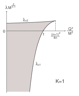
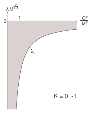
Figure 1: The parameter ranges in which the spacetime contains a regular black hole (the shaded regions).

In this section, we consider what we are able to conclude at this time about the stability of generalised static black holes with charge from the results of our formulation. In the present paper, we consider only the stability in the static region outside the black hole horizon with respect to a perturbation whose support is compact on the initial surface. This region is represented as $r>r_{H}$ for $\lambda\leq 0$ and $r_{H}<r<r_{c}$ for $\lambda>0$. As mentioned in §2.1, such a region exists only for restricted ranges of the parameters $M,Q$ and $\lambda$. These parameter ranges are shown in Fig. 1 (see Appendix A for details).

To study the stability in this region, as in Paper II, we utilize the fact that for any perturbation type, the perturbation equations in the static region of the spacetime are reduced to an eigenvalue problem of the type

$$\omega^{2}\Phi=A\Phi,$$ (166)

where $A$ is a self-adjoint operator,

$$A=-\frac{d^{2}}{dr_{*}^{2}}+V(r);\quad dr_{*}=\frac{dr}{f},$$ (167)

with $V(r)$ being equal to $V_{T}(r)$, $V_{V\pm}(r)$ or $V_{S\pm}(r)$. We regard the black hole to be stable if the spectrum of $A$, i.e., $\omega^{2}$, is non-negative.

To be precise, we must specify a boundary condition for $\Phi$ at $r=\infty$ in the case $\lambda<0$, for which the range of $r_{*}$ has an upper bound. In the present paper, we adopt the simplest condition, $\Phi\rightarrow 0$ as $r\rightarrow\infty$, in this case, which corresponds to the Friedrichs extension of $A$. For $\lambda\geq 0$, the range of $r_{*}$ is $(-\infty,+\infty)$ and the operator $A$ is essentially self-adjoint; i.e., it has a unique self-adjoint extension[32].

In general, if $\Phi(r)$ is a function with compact support contained in $r>r_{H}$ (or $r_{H}<r<r_{c}$ for $\lambda>0$), we can rewrite the expectation value of $A$, $(\Phi,A\Phi)$, as

$$(\Phi,A\Phi)=\int dr_{*}\left(\left|\frac{d\Phi}{dr_{*}}\right|^{2}+V|\Phi|^{2}\right).$$ (168)

For the Friedrichs extension of $A$, the lower bound of this quantity coincides with the lower bound of the spectrum of $A$ with domain $C^{\infty}_{0}(r_{*})$. Hence, if we can show that the right-hand side of (168) is non-negative, then we can conclude that the system is stable. In particular, if $V$ is non-negative, this condition is trivially satisfied. However, such a lucky situation is not realized in most cases. One powerful method that can be used to show the positivity of $A$ beyond such a simple situation is to deform the right-hand side of (168) by partial integration in terms of a function $S$ as

$$(\Phi,A\Phi)=\int dr_{*}\left(|\tilde{D}\Phi|^{2}+\tilde{V}|\Phi^{2}|\right),$$ (169)

where

$$\tilde{D}=\frac{d}{dr_{*}}+S,$$ (170)

$$\tilde{V}=V+f\frac{dS}{dr}-S^{2}.$$ (171)

We call this procedure the $S$-deformation of $V$ in this paper. As in Paper II, this is the main tool for the analysis in the present paper.

6.1 Tensor perturbation

If we apply the $S$-deformation with

$$S=-\frac{nf}{2r}$$ (172)

to (40), we obtain

$$\tilde{V}_{T}=\frac{f}{r^{2}}\left[\lambda_{L}-2(n-1)K\right],$$ (173)

irrespective of the $r$-dependence of $f(r)$. Hence, the effective potential $\tilde{V}_{T}$ is positive, and the system is perturbatively stable with respect to a tensor perturbation if

$$\lambda_{L}\geq 2(n-1)K.$$ (174)

In particular, this guarantees the stability of maximally symmetric black holes for $K=1$ and $K=0$, since $\lambda_{L}$ is related to the eigenvalue $k_{T}^{2}$ of the positive operator $-D\cdot D$ as $\lambda_{L}=k_{T}^{2}+2nK$ when ${\cal K}^{n}$ is maximally symmetric. In contrast, even in the maximally symmetric case, $\tilde{V}_{T}$ becomes negative in the range $0<k_{T}^{2}<2$ for $K=-1$, and we cannot conclude anything about the stability for $K=-1$ from this argument alone.

Note that the condition (174) is just a sufficient condition for stability, and it is not a necessary condition in general. In fact, for a tensor perturbation, we can obtain stronger stability conditions directly from the positivity of $V_{T}$ if we restrict the range of parameters. For example, for $K=1$ and $\lambda=0$, it is easy to see that $V_{T}$ is positive if

$$\lambda_{L}+2-2n+\frac{n(n-1)\sqrt{M^{2}-Q^{2}}}{M+\sqrt{M^{2}-Q^{2}}}\geq 0$$ (175)

for $M^{2}\geq Q^{2}>8n(n-1)M^{2}/(3n-2)^{2}$, and

$$\lambda_{L}+\frac{n^{2}-10n+8}{4}\geq 0$$ (176)

for $Q^{2}\leq 8n(n-1)M^{2}/(3n-2)^{2}$. Thus, if we do not restrict the range of $Q^{2}$, we obtain the same sufficient condition for stability as (174), but for the restricted range $Q^{2}\leq 8n(n-1)M^{2}/(3n-2)^{2}$, we obtain the stronger sufficient condition (176), which coincides with the condition obtained in Paper II for the case $Q=0$.

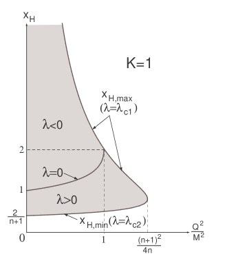
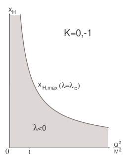
Figure 2: Ranges of the value $x_{H}$.

Similarly, for $K=-1$ and $\lambda<0$, rewriting $V_{T}$ as

$$V_{T}=\frac{f}{r^{2}}\left(\lambda_{L}-(3n-2)K+\frac{n(n+2)}{4}f+\frac{n(n+1)M}{r^{n-1}}-\frac{n^{2}Q^{2}}{r^{2n-2}}\right),$$ (177)

we obtain a sufficient condition for stability stronger than (174),

$$\lambda_{L}+3n-2=k_{T}^{2}+n-2\geq 0,$$ (178)

from $V_{T}>0$ if we restrict the range of $\lambda$ to

$$\lambda\geq-\left(\frac{(n+1)M}{nQ^{2}}\right)^{\frac{2}{n-1}}\left(1+\frac{(n^{2}-1)M^{2}}{n^{2}Q^{2}}\right).$$ (179)

This condition is sufficient to guarantee the stability of a maximally symmetric black hole with $K=-1$ for $n\geq 2$. However, if we extend the range of $\lambda$ to the whole allowed range, i.e., that satisfying $\lambda\geq\lambda_{c-}$, (174) is the strongest condition that can be obtained only from $V_{T}>0$.

6.2 Vector perturbation

For $V=V_{V\pm}$ in (79) and

$$S=\frac{nf}{2r},$$ (180)

we obtain

$$\tilde{V}_{V\pm}=\frac{f}{r^{2}}\left[m_{V}+\frac{(n^{2}-1)M\pm\Delta}{r^{n-1}}\right],$$ (181)

$$m_{V}=k_{V}^{2}-(n-1)K.$$ (182)

Hence, from $k_{V}^{2}\geq(n-1)K$, we find that $\tilde{V}_{V+}$ is always positive, and static charged black holes are stable with respect to the electromagnetic mode of the vector perturbation. In contrast, from

$$\tilde{V}_{V-}=\frac{f}{r^{2}}\frac{m_{V}h}{(n^{2}-1)M+\Delta},$$ (183)

$$h:=(n^{2}-1)M-\frac{2n(n-1)Q^{2}}{r^{n-1}}+\Delta,$$ (184)

it is seen that $\tilde{V}_{V-}$ may become negative: Because $h$ is a monotonically increasing function of $r$, $\tilde{V}_{V-}$ is positive if and only if $h(r_{H})\geq 0$.

6.2.1 The case $\lambda\geq 0$

In this case, the background spacetime contains a regular black hole only for $K=1$, and the static region outside the black hole is given by $r_{H}<r<r_{c}$ $(\leq+\infty)$. In this region, from (218b), we have $2M/r^{n-1}<x_{H}\leq x_{H,{\rm max}}\leq(n+1)M^{2}/(nQ^{2})$. Hence, $h>0$, and the black hole is stable in this case.

6.2.2 The case $\lambda<0$

In this case, as shown in Appendix A, the spacetime contains a regular black hole if $\lambda\geq\lambda_{c}$ and $2M/r^{n-1}<x_{H}\leq x_{H,{\rm max}}$. Hence, from (218b), we obtain the relation

$$h\geq\sqrt{(n^{2}-1)^{2}M^{2}+2n(n-1)m_{V}Q^{2}}-\sqrt{(n^{2}-1)^{2}M^{2}-4Kn(n-1)^{2}Q^{2}}.$$ (185)

For $K=0,1$, $h>0$ follows from this. Hence, the black hole is stable. In contrast, for $K=-1$, the right-hand side of this inequality becomes negative for $k_{V}^{2}<n-1$. Hence, $\tilde{V}_{V-}$ can become negative near the horizon if $\lambda$ is sufficiently close to $\lambda_{c-}$, provided that the spectrum of $k_{V}^{2}$ extends to $k_{V}^{2}<n-1$.

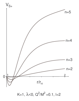
Figure 3: Examples of $V_{S+}$ for $K=1$ and $\lambda<0$.

6.3 Scalar perturbation

By applying the $S$-deformation to $V_{S+}$ with

$$S=\frac{f}{h_{+}}\frac{dh_{+}}{dr};\ h_{+}=r^{n/2-1}H_{+},$$ (186)

we obtain

$$\tilde{V}_{S+}=\frac{k^{2}f}{2r^{2}H_{+}}\left[(n-2)(n+1)\delta x+2\right].$$ (187)

Since this is positive definite, the electromagnetic mode $\Phi_{+}$ is always stable for any values of $K$, $M$, $Q$ and $\lambda$, provided that the spacetime contains a regular black hole, although $V_{S+}$ has a negative region near the horizon when $\lambda<0$ and $Q^{2}/M^{2}$ is small (see Fig. 3).

Using a similar transformation, we can also prove the stability of the gravitational mode $\Phi_{-}$ for some special cases. For example, the $S$-deformation of $V_{S-}$ with

$$S=\frac{f}{h_{-}}\frac{dh_{-}}{dr};\ h_{-}=r^{n/2-1}H_{-}$$ (188)

leads to

$$\tilde{V}_{S-}=\frac{k^{2}f}{2r^{2}H_{-}}\left[2m-(n+1)(n-2)(1+m\delta)x\right].$$ (189)

For $n=2$, this is positive definite for $m>0$. When $K=1$, $\lambda\geq 0$ and $n=3$ or when $\lambda\geq 0,Q=0$ and the horizon is $S^{4}$, from $m\geq n+2$ ($l\geq 2$) and the behaviour of $x_{h}$ (see Fig. 2), we can show that $\tilde{V}_{S-}>0$. Hence, in these special cases, the black hole is stable with respect to any type of perturbation.

However, for the other cases, $\tilde{V}_{S-}$ is not positive definite for generic values of the parameters. The $S$-deformation used to prove the stability of neutral black holes in Paper II is not effective either. This is because $V_{S-}$ has a negative region around the horizon for the extremal and near extremal cases, as shown in Fig. 4, and the $S$-deformation cannot remove this negative region if $S$ is a regular function at the horizon. Hence, determination of the stability for these generic cases with $n\geq 3$ is left as an open problem.

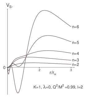
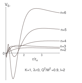
Figure 4: Examples of $V_{S-}$.

7 Summary and Discussion

In the present paper, we have extended the formulation for perturbations of a generalised static black hole given in Paper I to an Einstein-Maxwell system in a generalised static spacetime with a static electric field, and we have shown that the perturbation equations for vector and scalar perturbations can be reduced to two decoupled second-order ODEs for the gravitational mode and the electromagnetic mode, irrespective of the value of the cosmological constant and the curvature of the horizon. In particular, we have found that the coupling between the perturbations of the metric and the electromagnetic field produces significant modifications of the effective potentials for the gravitational mode and the electromagnetic mode when the black hole is charged. Our formulation also provides an extension of the corresponding formulation for the Reissner-Nordstrom black hole in four dimensions[33, 34, 35] to asymptotically de Sitter and anti-de Sitter cases.

Table 1: Stabilities of generalised static black holes. In this table, “$d$” represents the spacetime dimension, $n+2$. The results for tensor perturbations apply only for maximally symmetric black holes, while those for vector and scalar perturbations are valid for black holes with generic Einstein horizons, except in the case with $K=1,Q=0,\lambda>0$ and $d=6$.

		Tensor		Vector		Scalar
		$Q=0$	$Q\not=0$	$Q=0$	$Q\not=0$	$Q=0$	$Q\not=0$
$K=1$	$\lambda=0$	OK	OK	OK	OK	OK	$\begin{array}[]{l}d=4,5\ \text{OK}\\ d\geq 6\ \text{?}\end{array}$
	$\lambda>0$	OK	OK	OK	OK	$\begin{array}[]{l}d\leq 6\ \text{OK}\\ d\geq 7\ \text{?}\end{array}$	$\begin{array}[]{l}d=4,5\ \text{OK}\\ d\geq 6\ \text{?}\end{array}$
	$\lambda<0$	OK	OK	OK	OK	$\begin{array}[]{l}d=4\ \text{OK}\\ d\geq 5\ \text{?}\end{array}$	$\begin{array}[]{l}d=4\ \text{OK}\\ d\geq 5\ \text{?}\end{array}$
$K=0$	$\lambda<0$	OK	OK	OK	OK	$\begin{array}[]{l}d=4\ \text{OK}\\ d\geq 5\ \text{?}\end{array}$	$\begin{array}[]{l}d=4\ \text{OK}\\ d\geq 5\ \text{?}\end{array}$
$K=-1$	$\lambda<0$	OK	?	OK	?	$\begin{array}[]{l}d=4\ \text{OK}\\ d\geq 5\ \text{?}\end{array}$	$\begin{array}[]{l}d=4\ \text{OK}\\ d\geq 5\ \text{?}\end{array}$

With the help of this formulation and the method used in Paper II, we have analysed the stability of generalised static black holes with charge. The results are summarised in Table 1. As shown there, maximally symmetric black holes are stable with respect to tensor and vector perturbations over almost the entire parameter range; the exceptional case corresponds to a rather exotic black hole, whose horizon is a hyperbolic space. In contrast, for a scalar perturbation, we were not able to prove even the stability of asymptotically flat black holes with charge in generic dimensions, due to the existence of a negative region in the effective potential around the horizon in the extremal and near extremal cases, in contrast to the neutral case. Whether this negative ditch produces an unstable mode or not is uncertain. Hence, the stability of asymptotically flat and asymptotically de Sitter black holes for $d\geq 6$ and of asymptotically anti-de Sitter black holes for $d\geq 5$ are left as open problems. In connection to this, it should be noted that the existence of a negative region in the effective potential near the horizon may have a significant influence on the frequencies of the quasi-normal modes and the greybody factor for the Hawking process, even if these black holes are found to be stable.

In the present paper, we have also given explicit expressions for the source terms in the master equations. As mentioned in the introduction, this information will be necessary in the estimation of gravitational and electromagnetic emission from black holes in higher dimensions. In addition to this practical application, we also expect that these master equations with source terms can be used in the analysis of static singular perturbations of black holes associated with some singular source such as a string or a membrane. For example, if one treats the C-metric as a perturbation of a spherically symmetric solution, it is found that this perturbation obeys an equation with a string source. Hence, it is expected that one can obtain some information concerning higher-dimensional analogue of the C-metric by studying singular solutions to the master equation with a singular source.

Appendix A Parameter range for the existence of a regular black hole

In this section, we determine the parameter range in which the background metric (18) contains a regular black hole. Here, by a regular black hole, we mean a degenerate Killing horizon or bifurcating Killing horizons at $r=r_{H}$ that separate(s) a regular region with $f(r)>0$ and a singular region containing the singularity at $r=0$.

First, we consider parameter values satisfying $\lambda\geq 0$ and $K\leq 0$. In this range, if $Q=0$, there exists no horizon, because $f$ is negative everywhere. If $Q\neq 0$, from

$$(r^{n-1}f)^{\prime}=(n-1)Kr^{n-2}-(n+1)\lambda r^{n}-\frac{(n-1)Q^{2}}{r^{n}}<0,$$ (190)

$r^{n-1}f$ is a monotonically decreasing function of $r$. Further,

$$r^{n-1}f\rightarrow\left\{\begin{array}[]{ll}+\infty,&r\rightarrow+0\\ \leq-2M,&r\rightarrow+\infty\end{array}\right..$$ (191)

Hence, the spacetime has no region with $f>0$ that is separated from the singular region by Killing horizons. Therefore, the spacetime contains regular black holes only for $K=1$ or $\lambda<0$.

A.1 The case $Q=0$

In this case, since $f\rightarrow-\infty$ as $r\rightarrow+0$, the spacetime contains a regular black hole if there is a region in which $f>0$. From

$$f^{\prime}=-2\lambda r+\frac{2(n-1)M}{r^{n}},$$ (192)

it is seen that the result depends on $\lambda$.

A.1.1 $\lambda<0$ or $K=1$ and $\lambda=0$

Because $f$ is monotonically increasing and becomes positive as $r\rightarrow+\infty$, $f$ has a single zero at $r=r_{H}$, and $f>0$ for $r>r_{H}$. Thus, there is a regular black hole.

A.1.2 $K=1$ and $\lambda>0$

Because $f$ has a single maximum at $r=a$, the spacetime contains a regular black hole if and only if $f(a)>0$. Then, since $f^{\prime}(a)=0$ is equivalent to

$$\lambda=\frac{(n-1)M}{a^{n+1}},$$ (193)

this condition can be written as

$$a^{n-1}>(n+1)M.$$ (194)

In terms of $\lambda$, it is expressed as

$$\lambda<\frac{n-1}{n+1}\frac{1}{[(n+1)M]^{\frac{2}{n-1}}}.$$ (195)

$f$ has two zeros, at $r=r_{H}$ and $r=r_{c}$ ($r_{H}<r_{c}$), and $f>0$ for $r_{H}<r<r_{c}$,

A.2 The case $Q\not=0$

When $Q\not=0$, since $f\rightarrow+\infty$ as $r\rightarrow+0$, there must exist a point $r=a$ such that $f^{\prime}(a)=0$ and $f(a)\leq 0$ in order for the spacetime to contain a regular black hole. From

$$f^{\prime}=-2\lambda r+2(n-1)\left(\frac{M}{r^{n}}-\frac{Q^{2}}{r^{2n-1}}\right),$$ (196)

$\lambda$ is expressed in terms of $a$ as

$$\lambda=g(a):=\frac{(n-1)}{a^{2}}\left(\frac{M}{a^{n-1}}-\frac{Q^{2}}{a^{2n-2}}\right).$$ (197)

From this, $f(a)$ can be written as

$$f(a)=K-\frac{(n+1)M}{a^{n-1}}+\frac{nQ^{2}}{a^{2n-2}}.$$ (198)

Hence, the condition $f(a)\leq 0$ requires

$$D:=(n+1)^{2}M^{2}-4KnQ^{2}\geq 0,$$ (199)

and under this condition, $f(a)\leq 0$ if $a$ satisfies

$$\max\left(0,\frac{(n+1)M-\sqrt{D}}{2nQ^{2}}\right)\leq\frac{1}{a^{n-1}}\leq\frac{(n+1)M+\sqrt{D}}{2nQ^{2}}.$$ (200)

Note that $g(a)$ has a maximum at $a=a_{m}$, where

$$a_{m}^{n-1}=\frac{2nQ^{2}}{(n+1)M},$$ (201)

and it is monotonic everywhere except at this point. Further, $g(+0)=-\infty$ and $g(+\infty)=0$. Hence, $\lambda<0$ for $a<a_{0}$, where

$$a_{0}^{n-1}=\frac{Q^{2}}{M},$$ (202)

and $\lambda>0$ for $a>a_{0}$.

A.2.1 $K=1$ and $\lambda=0$

In this case, the spacetime contains a regular black hole if and only if $M^{2}\geq Q^{2}$, and the horizon is at $r^{n-1}=r_{H}^{n-1}=M+\sqrt{M^{2}-Q^{2}}$.

A.2.2 $K=1$ and $\lambda>0$

Because the sign of $f^{\prime}(r)$ is the same as the sign of $g(r)-\lambda$, the condition that there is a point $r=a$ such that $f^{\prime}(a)=0$ is equivalent to the relation

$$\lambda\leq\lambda_{\rm{max}}:=g(a_{m})=\frac{(n+1)(n-1)^{2}}{4n^{2}}\left(\frac{n+1}{2n}\right)^{\frac{2}{n-1}}\left(\frac{M^{2}}{Q^{2}}\right)^{\frac{n+1}{n-1}}\frac{1}{M^{\frac{2}{n-1}}}.$$ (203)

Further, from the condition $D\geq 0$, we have

$$\frac{Q^{2}}{M^{2}}\leq\frac{4n}{(n+1)^{2}}.$$ (204)

Under these conditions, $f^{\prime}(a)=0$ has in general two solutions, $a=a_{1},a_{2}$ $(a_{0}<a_{1}<a_{m}<a_{2})$, and the spacetime contains a regular black hole if and only if $f(a_{1})\leq 0<f(a_{2})$.

First, from $f(a_{2})>0$, we obtain

$$a_{2}^{n-1}>\frac{(n+1)M+\sqrt{D}}{2}=:a_{c2}^{n-1}.$$ (205)

In terms of $\lambda$, this can be expressed as

$$\lambda<\lambda_{c2}:=g(a_{c2})=2^{\frac{n+1}{n-1}}\frac{n-1}{n}\frac{(n-1)M+\sqrt{D}}{[(n+1)M+\sqrt{D}]^{\frac{n+1}{n-1}}}.$$ (206)

Next, because $f(a)$ becomes minimal at $a=a_{m}$, from $f(a_{0})=1-M^{2}/Q^{2}$, we have $f(a_{1})\leq f(a_{0})\leq 0$ if $Q^{2}\leq M^{2}$. Also, for $M^{2}<Q^{2}\leq(n+1)^{2}/(4n)M^{2}$, $f(a_{1})\leq 0$ is equivalent to

$$a_{1}^{n-1}\leq\frac{(n+1)M-\sqrt{D}}{2}=:a_{c1}^{n-1},$$ (207)

or, in terms of $\lambda$, to

$$\lambda\geq\lambda_{c1}:=g(a_{c1})=2^{\frac{n+1}{n-1}}\frac{n-1}{n}\frac{(n-1)M-\sqrt{D}}{[(n+1)M-\sqrt{D}]^{\frac{n+1}{n-1}}}.$$ (208)

Here, if we vary $Q^{2}$ with $M$ fixed, we have

$$\frac{d}{da_{c1}}(\lambda_{c2}-\lambda_{c1})=\frac{(n-1)\sqrt{D}}{n}\left(\frac{1}{a_{c2}^{n+2}}-\frac{1}{a_{c1}^{n+2}}\right)<0.$$ (209)

Hence, $\lambda_{c2}-\lambda_{c1}$ is a monotonically increasing function of $Q$ for fixed $M$, and $\lambda_{c1}=\lambda_{c2}$ at $Q^{2}=(n+1)^{2}M^{2}/(4n)$. From these results, it follows that $\lambda_{c1}<\lambda_{c2}$ for $Q^{2}<(n+1)^{2}/(4n)M^{2}$. Further, $\lambda_{c1}$ vanishes at $Q^{2}=M^{2}$. Therefore, for $\lambda>0$ and $K=1$, the spacetime contains a regular black hole if and only if

$$\max\left(0,\lambda_{c1}\right)\leq\lambda<\lambda_{c2}:\ Q^{2}<\frac{(n+1)^{2}M^{2}}{4n}.$$ (210)

Table 2: The parameter range in which the spacetime contains a regular black hole.

	$K=1$	$K=0$	$K=-1$
$\lambda=0$	$Q^{2}\leq M^{2}$	$\not\exists$	$\not\exists$
$\lambda>0$	For $Q^{2}\leq M^{2}$
	$\lambda<\lambda_{c2}$	$\not\exists$	$\not\exists$
	For $M^{2}<Q^{2}<(n+1)^{2}M^{2}/(4n)$
	$\lambda_{c1}\leq\lambda<\lambda_{c2}$
$\lambda<0$	$Q^{2}<M^{2}$ and $\lambda_{c1}\leq\lambda$	$\lambda_{c0}\leq\lambda$	$\lambda_{c-}\leq\lambda$

A.2.3 $\lambda<0$

In this case, $f^{\prime}(a)=0$ always has a single solution, and $f\rightarrow+\infty$ as $r\rightarrow+0,+\infty$. Hence, the spacetime contains a regular black hole if and only if $f(a)\leq 0$. Because $a<a_{0}<a_{m}$, this condition is equivalent to

$$\frac{1}{a^{n-1}}\leq\frac{1}{a_{c}^{n-1}}\equiv\frac{(n+1)M+\sqrt{D}}{2nQ^{2}},$$ (211)

or in terms of $\lambda$,

$$\lambda\geq\lambda_{c}=\frac{n-1}{na_{c}^{2}}\left(K-\frac{M}{a_{c}^{n-1}}\right).$$ (212)

This, together with $D\geq 0$, leads to the following conditions:

$$K=0: \lambda>\lambda_{c0}:=-\frac{n^{2}-1}{n^{2}}\left(\frac{n+1}{n}\right)^{\frac{2}{n-1}}\left(\frac{M^{2}}{Q^{2}}\right)^{\frac{n+1}{n-1}}\frac{1}{M^{\frac{2}{n-1}}},$$ (213a)

$$K=-1: \lambda>\lambda_{c-}:=-2^{\frac{2}{n-1}}\frac{n-1}{n}\frac{\sqrt{D}-(n-1)M}{[\sqrt{D}-(n+1)M]^{\frac{n+1}{n-1}}},$$ (213b)

$$K=1: \lambda>\lambda_{c1}:=-2^{\frac{2}{n-1}}\frac{n-1}{n}\frac{\sqrt{D}-(n-1)M}{[(n+1)M-\sqrt{D}]^{\frac{n+1}{n-1}}}.$$ (213c)

Finally, we determine the range of $x_{H}=2M/r_{H}^{n-1}$. In general, $\lambda$ is expressed in terms of $r_{H}$ as

$$\lambda=\frac{1}{r_{H}^{2}}\left(K-\frac{2M}{r_{H}^{n-1}}+\frac{Q^{2}}{r_{H}^{2n-2}}\right).$$ (214)

From this, we have

$$\frac{d\lambda}{dr_{H}}=-\frac{2}{r^{3}}\left(K-\frac{(n+1)M}{r_{H}^{n-1}}+\frac{n^{2}Q^{2}}{r_{H}^{2n-2}}\right).$$ (215)

First, for $K=1$, this can be written in terms of $a_{c1}$ and $a_{c2}$ as

$$\frac{d\lambda}{dr_{H}}=\frac{2nQ^{2}}{r_{H}^{2}}\left(\frac{1}{a_{c1}^{n-1}}-\frac{1}{r_{H}^{n-1}}\right)\left(\frac{1}{r_{H}^{n-1}}-\frac{1}{a_{c1}^{n-1}}\right).$$ (216)

From this and the relation $a_{c2}<a_{2}<r_{H}<a_{1}<a_{c1}$, it follows that $\lambda$ is a monotonically increasing function of $r_{H}$ for fixed $M$ and $Q$. Hence, from the constraint $\lambda_{c1}\leq\lambda<\lambda_{c2}$, we obtain

$$x_{H,\min}<x_{H}\leq x_{H,\max},$$ (217)

where $x_{H,\min}$ and $x_{H,\max}$ are the values of $x_{H}$ for $\lambda=\lambda_{c2}$ and $\lambda=\lambda_{c1}$, respectively:

$$x_{H,\min}=\frac{4M}{(n+1)M+\sqrt{D}},$$ (218a)

$$x_{H,\max}=\frac{(n+1)M^{2}+M\sqrt{D}}{nQ^{2}}.$$ (218b)

Next, for $K=0$ or $K=-1$, $d\lambda/dr_{H}$ can be written in terms of $a_{c}$ as

$$\frac{d\lambda}{dr_{H}}=\frac{2nQ^{2}}{r_{H}^{2}}\left(\frac{1}{a_{c}^{n-1}}-\frac{1}{r_{H}^{n-1}}\right)\left(\frac{1}{r_{H}^{n-1}}+\frac{\sqrt{D}-(n+1)M}{2nQ^{2}}\right).$$ (219)

From $r_{H}\leq a\leq a_{c}$, this is non-negative. Hence, from $\lambda_{c}\leq\lambda<0$, we obtain

$$0<x_{H}\leq x_{H,\max}.$$ (220)

The allowed ranges of $x_{H}$ given in (217) and (220) in the $(x_{H},Q^{2}/M^{2})$ plane are displayed in Fig. 2.

Appendix B Expressions for $\hat{E}^{t}_{t}$ and $\hat{E}_{L}$

We have the following expressions for $\hat{E}^{t}_{t}$ and $\hat{E}_{L}$:

$$2\hat{E}^{t}_{t}= -f\partial_{r}^{2}(X+S_{T})+\left(\frac{n-4}{r}f-\frac{f^{\prime}}{2}\right)\partial_{r}(X+S_{T})$$ (221)

$$+\left[\frac{k^{2}+(n-2)K}{r^{2}}+\frac{(n-2)(n-3)M}{r^{n+1}}\right.$$

$$\quad\qquad\left.-3(n-1)\lambda+\frac{(2n-3)Q^{2}}{r^{2n}}\right](X+S_{T})$$

$$-f\partial_{r}^{2}Y-\left(\frac{4f}{r}+\frac{f^{\prime}}{2}\right)\partial_{r}Y$$

$$+\left[-\frac{2K}{r^{2}}-\frac{(n-2)(n+3)M}{r^{n+1}}+3\lambda+\frac{(n+1)(2n-3)Q^{2}}{r^{2n}}\right]Y,$$

$$2\hat{E}_{L}= \frac{1}{f}\partial_{t}^{2}X+\frac{f^{\prime}}{2}\partial_{r}X$$ (222)

$$+\left[-\frac{(n-1)(n-2)M}{r^{n+1}}-3\lambda+\frac{n(n-1)Q^{2}}{r^{2n}}\right]X$$

$$-f\partial_{r}^{2}Y-\left(\frac{2f}{r}+\frac{3f^{\prime}}{2}\right)\partial_{r}Y$$

$$+\left[\frac{(n-1)(n-2)M}{r^{n+1}}+3\lambda-\frac{3(n-1)(n-2)Q^{2}}{r^{2n}}\right]Y$$

$$+\frac{2}{f}\partial_{t}\partial_{r}Z+\left(\frac{2}{rf}-\frac{f^{\prime}}{rf^{2}}\right)\partial_{t}Z$$

$$-f\partial_{r}^{2}S_{T}+\left(\frac{n-3}{r}f-f^{\prime}\right)\partial_{r}S_{T}$$

$$+\left[\frac{(n-1)k^{2}}{nr^{2}}+\frac{2(n-1)(n-2)M}{r^{n+1}}\right.$$

$$\quad\qquad\left.-3(n-1)\lambda-\frac{2(n-1)(n-3)Q^{2}}{r^{2n}}\right]S_{T}.$$

Appendix C Expressions for coefficient functions

We have the following:

$$P_{S1}= \left[-4n^{4}z+2n^{2}(n+1)x-4n(n-2)m\right]y$$ (224)

$$+\left\{2n^{2}(n-1)x+4n(n-2)m+4n^{3}(n-2)K\right\}z$$

$$-n^{2}(n^{2}-1)x^{2}+\left\{-4n(n-2)m+2n^{2}(n+1)K\right\}x$$

$$+4m^{2}+4n^{2}mK,$$

$$P_{S2}= \left[6n^{4}z-n^{2}(n+1)(n+2)x+2n(n-4)m\right]y$$

$$-2n^{4}z^{2}+\left\{n^{2}(3n^{2}-n+2)x-4n(n-2)m-6n^{3}(n-1)K\right\}z$$

$$-n^{2}(n+1)x^{2}+\left\{n(3n-7)m+n^{2}(n^{2}-1)K\right\}x$$

$$-2m^{2}-2n(n-1)mK,$$

$$P_{S3}= -2n^{2}(3n-2)z+n^{2}(n+1)x-2(n-2)m.$$ (225)

$$P_{X0}= \left[4n^{2}(n^{2}-1)(n^{2}z+m)x-8n^{4}(n-1)(3n-2)z^{2}\right.$$ (230)

$$\quad\left.-32n^{2}(n-1)^{2}mz-8(n-1)(n-2)m^{2}\right]y$$

$$+n^{3}(n+1)^{3}x^{3}+2n(n+1)\left\{-n^{2}(3n-1)(n+2)z\right.$$

$$\qquad\left.+2(n^{2}+n+2)m-n(n-2)(n+1)K\right\}x^{2}$$

$$+\left[4n^{4}(13n-7)z^{2}-4n^{2}\left\{(9n^{2}-8n+15)m+n(n+1)(n^{2}-7n+8)K\right\}z\right.$$

$$\quad\left.-4n(n-11)m^{2}-4n^{2}(n+1)(n-3)mK\right]x$$

$$-8n^{4}(3n-2)z^{3}+8n^{2}\left\{4(n^{2}-n+1)m+n^{2}(3n-4)(n-2)K\right\}z^{2}$$

$$+\left\{(16n^{2}-72n+16)m^{2}+16n^{3}(2n-3)mK\right\}z$$

$$+8n^{2}m^{2}K+16m^{3},$$

$$P_{X1}= \left[4n^{2}(n-1)z+4(n-1)m\right]y$$

$$+n(n+1)^{2}x^{2}+\left\{-8n^{2}z+2(3n-1)m-2n(n+1)K\right\}x$$

$$+4n^{2}z^{2}-\left\{4(2n-1)m+4n^{2}(n-2)K\right\}z-4nmK,$$

$$P_{Y0}= \left[2n^{4}(n+1)^{2}x^{2}-4n^{2}(n+1)\left\{n^{2}(5n-3)z+(n-3)m\right\}x\right.$$

$$\quad\left.+8n^{4}(2n-1)(3n-2)z^{2}+16n^{2}(n^{2}-4n+2)mz-8(n-2)m^{2}\right]y$$

$$+n^{3}(n-1)(n+1)^{2}x^{3}$$

$$+2n(n^{2}-1)\left\{-2n^{2}(3n-1)z+4m-n(n-2)(n+1)K\right\}x^{2}$$

$$+\left[20n^{4}(2n-1)(n-1)z^{2}+4n^{2}(n-1)\left\{(n-13)m+n(5n-8)(n+1)K\right\}z\right.$$

$$\qquad\left.+12n(n-1)m^{2}+4n^{2}(n^{2}-1)mK\right]x$$

$$-8n^{4}(3n-2)(n-1)z^{3}+16n^{2}(n-1)\left\{2m-n^{2}(3n-4)K\right\}z^{2}$$

$$-8(n-1)m\left\{(5n-2)m+2n^{3}K\right\}z,$$

$$P_{Y1}= \left[2n^{2}(n+1)x-4n^{2}(2n-1)z+4m\right]y$$

$$+n(n^{2}-1)x^{2}-2(n-1)\left\{3n^{2}z+m+n(n+1)K\right\}x$$

$$+4n^{2}(n-1)z^{2}+4(n-1)(m+2n^{2}K)z,$$

$$P_{Z}= \left[-n^{2}(n+1)x+2n^{2}(3n-2)z+2(n-2)m\right]y$$

$$+n(n+1)x^{2}+\left\{n^{2}(3n-7)z+(4n-2)m+n(n+1)(n-2)K\right\}x$$

$$-2n^{2}(n-2)z^{2}-\left\{(6n-4)m+2n^{2}(3n-4)K\right\}z-2nmK.$$

Note that these functions satisfy the following relations:

$$P_{X0}+P_{Y0}+4nHP_{Z}=16H^{3},$$ (231a)

$$P_{X1}+P_{Y1}=-4nrfH.$$ (231b)

$$P_{XA}= \left[4n^{3}(n-1)z+4n(n-1)m\right]y$$ (232)

$$+n^{2}(n+1)^{2}x^{2}+4n\left\{-2n^{2}z+(n-1)m-n(n+1)K\right\}x$$

$$+4n^{3}z^{2}-4n\left\{(n-1)m+n^{2}(n-3)K\right\}z$$

$$-4m^{2}-4n(n+1)mK,$$

$$P_{X2}= \left[4(n-1)n^{2}z+4(n-1)m\right]y$$ (233)

$$+n(n+1)^{2}x^{2}+\left\{-8n^{2}z+(6n-2)m-2n(n+1)K\right\}x$$

$$+4n^{2}z^{2}-\left\{4(2n-1)m+4n^{2}(n-2)K\right\}z-4nmK,$$

$$P_{X3}= (n+1)x+2n(n-2)z+2m,$$ (234)

$$P_{YA}= \left[2n^{3}(n+1)x-4n^{3}(2n-1)z+4nm\right]y$$ (235)

$$+n^{2}(n^{2}-1)x^{2}+\left\{-6n^{3}(n-1)z+4nm-2n^{2}(n+1)(n-2)K\right\}x$$

$$+4n^{3}(n-1)z^{2}+4n\left\{-m+n^{2}(2n-3)K\right\}z+4nmK+4m^{2},$$

$$P_{Y2}= \left[2n^{2}(n+1)x-4n^{2}(2n-1)z+4m\right]y$$ (236)

$$+n(n^{2}-1)x^{2}-2(n-1)\left\{3n^{2}z+m+n(n+1)K\right\}x$$

$$+4n^{2}(n-1)z^{2}+4(n-1)(m+2n^{2}K)z,$$

$$P_{Y3}=(n-1)\left[(n+1)x-4nz\right].$$ (237)

The following relations hold for these functions:

$$P_{XA}+P_{YA}=-4n^{2}fH,\quad P_{X2}+P_{Y2}=-4nfH,\quad P_{X3}+P_{Y3}=2H.$$ (238)

Appendix D Gauge-invariant treatment of the exceptional modes

In the present paper, we imposed the Einstein equation $F^{a}_{a}+2(n-2)F=0$ as the gauge condition for the exceptional modes of the scalar perturbation with $k^{2}=n$ for $K=1$. As discussed in Paper I, this gauge condition does not fix the gauge freedom completely, and it leaves the residual gauge freedom represented by $\bar{\delta}z^{i}=L{\mathbb{S}}^{i}$ satisfying

$$\frac{1}{r^{n}}D\cdot(r^{n}DL)+\frac{n-2}{r^{2}}L=0.$$ (239)

Hence, the master variables introduced in §5 contain unphysical degrees of freedom for the exceptional modes, although the master equations themselves are gauge-invariant. In this appendix, we express the master equations in terms of genuinely gauge-invariant variables.

We define all quantities for an exceptional mode corresponding to the gauge-invariant variables for a generic mode introduced in the text by the same expressions with $H_{T}=0$. Then, for the general gauge transformation (31), $X_{a}$ transforms as $X_{a}\rightarrow X_{a}+\bar{\delta}X_{a}$ with

$$\bar{\delta}X_{a}=-r^{2}D_{a}(L/k)+T_{a}.$$ (240)

From this, the following transformation laws of $F$ and $F^{a}_{b}$ are obtained:

$$F\rightarrow F+\bar{\delta}F: \bar{\delta}F=-rDr\cdot D(L/k)-L/k,$$ (241a)

$$F_{ab}\rightarrow F_{ab}+\bar{\delta}F_{ab}: \bar{\delta}F_{ab}=-D_{a}\left(r^{2}D_{b}\frac{L}{k}\right)-D_{b}\left(r^{2}D_{a}\frac{L}{k}\right).$$ (241b)

In particular, we have

$$\bar{\delta}(F^{c}_{c}-2nF)=-2\left[r^{n}D\cdot\left(\frac{D(L/k)}{r^{n-2}}\right)-n\frac{L}{k}\right].$$ (242)

Hence, from (32) and (95), ${\cal E}$ and ${\cal E}_{a}$ transform as

$$\bar{\delta}{\cal E}=-D\cdot\left(r^{2}E_{0}D(L/k)\right)=-qD\cdot\left(\frac{D(L/k)}{r^{n-2}}\right),$$ (243a)

$$\bar{\delta}{\cal E}_{a}=rE_{0}D_{a}L=\frac{q}{r^{n-1}}D_{a}L.$$ (243b)

From this and the definition of ${\cal A}$, (104), we find that ${\cal A}$ transforms as

$$\bar{\delta}{\cal A}=q\frac{L}{k}.$$ (244)

Like these variables, the matter variables $\Sigma_{ab},\Sigma_{a}$ and $\Sigma_{L}$ are gauge dependent. However, $S_{a},S^{a}_{b}$ and $S_{L}$ are gauge-invariant, because they represent perturbations of quantities whose background values vanish, like $J_{a}$.

In order to proceed further, we have to treat the black-hole-type background case and the Nariai-type background case separately.

D.1 Black hole background

In the black hole background (18), the gauge transformation of $F^{a}_{b}$ is written

$$\bar{\delta}F^{t}_{t}=-\frac{2\omega^{2}r^{2}}{f}\frac{L}{k}-r^{2}f^{\prime}\frac{L^{\prime}}{k},$$ (245a)

$$\bar{\delta}F^{r}_{t}=i\omega\left[2r^{2}f\frac{L^{\prime}}{k}+2r\left(f-\frac{rf^{\prime}}{2}\right)\frac{L}{k}\right],$$ (245b)

$$\bar{\delta}F^{r}_{r}=-2r^{2}f(L^{\prime\prime}/k)-r(4f+rf^{\prime})(L^{\prime}/k).$$ (245c)

In particular, we have

$$\bar{\delta}\left(2F+\frac{F^{r}_{t}}{i\omega r}\right)=-\frac{2H}{n}\frac{L}{k}.$$ (246)

Hence, the master variable $\Phi$ transforms as

$$\bar{\delta}\Phi=-2r^{n/2}\frac{L}{k}.$$ (247)

For $k^{2}=n$ and $K=1$, $\mu=M$ and $\Phi_{\pm}$ are written

$$\Phi_{+}=\frac{(n+1)MQ}{r^{n/2-1}}\left(\frac{\Phi}{r^{n/2}}+\frac{2{\cal A}}{q}\right),$$ (248a)

$$\Phi_{-}=\left(2(n+1)M-\frac{2nQ^{2}}{r^{n-1}}\right)\Phi-\frac{4nQ^{2}}{r^{n/2-1}}\frac{{\cal A}}{q}.$$ (248b)

From this, we find that $\Phi_{+}$ is gauge-invariant. In contrast, as is seen from the relation

$$\Phi=\frac{\Phi_{-}}{2(n+1)M}+\frac{n\sqrt{\delta}}{(n+1)M}\Phi_{+},$$ (249)

$\Phi_{-}$ is not gauge-invariant. Nevertheless, the master equation for $\Phi_{-}$ is gauge-invariant. This becomes evident if we rewrite this equation in terms of the gauge-invariant combinations

$$\hat{F}^{t}_{t}:=F^{t}_{t}-\frac{1}{r^{n/2}}\left[\frac{r^{2}f^{\prime}}{2}\Phi^{\prime}+\left(\frac{\omega^{2}r^{2}}{f}-\frac{nrf^{\prime}}{4}\right)\Phi\right],$$ (250a)

$$\hat{F}^{r}_{t}:=F^{r}_{t}+\frac{i\omega r}{r^{n/2}}\left[rf\Phi^{\prime}-\frac{(n-2)f+rf^{\prime}}{2}\Phi\right],$$ (250b)

$$\hat{F}^{r}_{r}:=F^{r}_{r}-\frac{1}{r^{n/2}}\Big{[}r^{2}f\Phi^{\prime\prime}-\frac{2(n-2)rf-r^{2}f^{\prime}}{2}\Phi^{\prime}$$

$$\qquad\qquad+\frac{n(n-2)f-nrf^{\prime}}{4}\Phi\Big{]},$$ (250c)

$$\hat{F}:=F-\frac{1}{2r^{n/2}}\left[rf\Phi^{\prime}+\left(1-\frac{nf}{2}\right)\Phi\right].$$ (250d)

Then, taking account of the fact that the master equation was derived under the gauge condition $F^{a}_{a}+2(n-2)F=0$, we obtain

$$\hat{F}^{a}_{a}+2(n-2)\hat{F}=-\frac{1}{2(n+1)Mr^{n/2-2}f}\left[S_{s-}+2n\sqrt{\delta}S_{s+}+2n\sqrt{\delta}(V_{s+}-V_{s-})\Phi_{+}\right].$$ (251)

Here, for $k^{2}=n$ and $K=1$, we have

$$V_{s+}-V_{s-}= \frac{(n-1)f}{2r^{2}H_{+}^{2}}\big{[}\left\{4-2n^{2}(n+1)\delta x\right\}y$$ (252)

$$+\delta(n^{2}-1)x^{2}+\{2n(n+1)(n-2)\delta-2n+2\}x].$$

Since this equation is written only in terms of gauge-invariant variables, it is valid in any gauge. Thus, the master equation for $\Phi_{-}$ gives an algebraic relation among the gauge-invariant variables $\Phi_{+}$, $\hat{F}$ and $\hat{F}^{a}_{b}$.

The definition of $\Phi$ yields another relation,

$$2i\omega r\hat{F}+\hat{F}^{r}_{t}=0.$$ (253)

Further, the expressions (130) for $X$ and $Z$ provide two more relations:

$$r^{n-2}(\hat{F}^{t}_{t}-2\hat{F})=\frac{n^{2}(n-1)Q}{2(n+1)Mr^{n/2+1}}\left(\frac{nP_{X+}}{2H^{2}}\Phi_{+}-\frac{2rf}{H}\Phi_{+}^{\prime}\right)+X_{s}|_{{\cal A}=0},$$ (254a)

$$r^{n-2}\hat{F}^{r}_{t}=-i\omega\frac{n^{2}(n-1)Qf}{(n+1)Mr^{n/2}H}\Phi_{+}+Z_{s}|_{{\cal A}=0},$$ (254b)

where

$$P_{X+}= \left[(n+1)(n-2)x+2n^{2}z\right]y+(n+1)(2n-1)x^{2}$$ (255)

$$-\{(3n^{2}+3n-2)z+(n+1)(n+2)\}x+2n^{2}z^{3}-2n(n-4)z.$$

The four equations (252), (253) and (254) can be solved to yield expressions for $\hat{F}$ and $\hat{F}^{a}_{b}$ in terms of $\Phi_{+}$ and the gauge-invariant matter source terms $S_{a}$, $S^{a}_{b}$ and $\tilde{J}_{a}$. Therefore, the only dynamical gauge-invariant variable for the exceptional modes is $\Phi_{+}$. Note that we can impose the gauge condition $\Phi=0$, and for this gauge, $\hat{F}^{a}_{b}=F^{a}_{b}$ and $\hat{F}=F$ hold and $\Phi_{+}$ is proportional to ${\cal A}$.

D.2 Nariai-type background

The case of the Nariai-type background can be treated in almost the same way. First, the gauge transformations of $F^{a}_{b}$ and $F$ are written

$$\bar{\delta}F^{t}_{t}=-2a^{2}\left(\frac{\omega^{2}}{f}\frac{L}{k}+\frac{f^{\prime}}{2}\frac{L^{\prime}}{k}\right),$$ (256a)

$$\bar{\delta}F^{\rho}_{t}=2ia^{2}\omega\left(f\frac{L^{\prime}}{k}-\frac{f^{\prime}}{2}\frac{L}{k}\right),$$ (256b)

$$\bar{\delta}F^{\rho}_{\rho}=-2a^{2}\left(f\frac{L^{\prime\prime}}{k}+\frac{f^{\prime}}{2}\frac{L^{\prime}}{k}\right),$$ (256c)

$$\bar{\delta}F=-\frac{L}{k}.$$ (256d)

For $m=0$ and $K=1$, $\sigma$ and $\mu$ have the simple expressions

$$\sigma=\frac{n-1}{a^{2}}-\frac{n(n-1)Q^{2}}{a^{2n}},$$ (257a)

$$\mu=\frac{n-1}{a^{2}}+\frac{n(n-1)Q^{2}}{a^{2n}}.$$ (257b)

Hence, $\Phi_{\pm}$ are written

$$\Phi_{+}=\frac{2(n-1)Q}{a^{2}}\left(F+\frac{{\cal A}}{q}\right),$$ (258a)

$$\Phi_{-}=\frac{2(n-1)}{a^{2}}\left(F-\frac{nQ^{2}}{a^{2n-2}}\frac{{\cal A}}{q}\right).$$ (258b)

From this, we find that $\Phi_{+}$ is gauge-invariant, while $\Phi_{-}$ is not gauge-invariant, as seen from the relation

$$F=\frac{1}{2\mu}\left(\Phi_{-}+\frac{nQ}{a^{2n-2}}\Phi_{+}\right),$$ (259)

as in the black hole background case.

We can construct the following gauge-invariant quantities from $F^{a}_{b}$ and $F$:

$$\hat{F}^{t}_{t}=F^{t}_{t}-2a^{2}\left(\frac{\omega^{2}}{f}F+\frac{f^{\prime}}{2}F^{\prime}\right),$$ (260a)

$$\hat{F}^{\rho}_{t}=F^{\rho}_{t}+2i\omega a^{2}\left(fF^{\prime}-\frac{f^{\prime}}{2}F\right),$$ (260b)

$$\hat{F}^{\rho}_{\rho}=F^{\rho}_{\rho}-2a^{2}\left(fF^{\prime\prime}+\frac{f^{\prime}}{2}F^{\prime}\right).$$ (260c)

Under the gauge condition $F^{a}_{a}+2(n-2)F=0$, we have

$$\hat{F}^{a}_{a}=-\frac{2a^{2}}{f}\left[f(fF^{\prime})^{\prime}+\left(\omega^{2}+\frac{n-2}{a^{2}}f\right)F\right].$$ (261)

From this, it follows that the master equation for $\Phi_{-}$ can be expressed in terms of the gauge invariant variables as

$$\hat{F}^{a}_{a}=-\frac{a^{2}}{\mu f}\left(S_{-}+\frac{nQ}{a^{2n-2}}S_{+}\right)-\frac{nQ}{a^{2n-4}}\Phi_{+}.$$ (262)

Further, the equations for $X$ and $Z$ can be rewritten as

$$\hat{F}^{t}_{t}=-\frac{nQ}{a^{2n-4}}-\frac{2}{na^{n-4}}S^{\rho}_{\rho},$$ (263a)

$$\hat{F}^{\rho}_{t}=\frac{2}{na^{n-4}}S^{\rho}_{t}.$$ (263b)

The corresponding expression for $\hat{F}^{\rho}_{\rho}$ can be obtained from those for $\hat{F}^{t}_{t}$ and $\hat{F}^{a}_{a}$. Under the gauge condition $F=0$, $\hat{F}^{a}_{b}$ coincides with $F^{a}_{b}$, and $\Phi_{+}$ becomes a constant multiple of ${\cal A}$.

References

- [1] Arkani-Hamed, N., Dimopoulos, S. and Dvali, G.: The Hierarchy Problem and New Dimensions at a Millimeter, Phys. Lett. B 429, 263–272 (1998).
- [2] Antoniadis, I., Arkani-Hamed, N., Dimopoulos, S. and Dvali, G.: New Dimensions at a Millimeter to a Fermi and Superstrings at a TeV, Phys. Lett. B 436, 257–263 (1998).
- [3] Randall, L. and Sundrum, R.: Large mass hierarchy from a small extra dimension, Phys. Rev. Lett. 83, 3370 (1999).
- [4] Randall, L. and Sundrum, R.: An alternative to compactification, Phys. Rev. Lett. 83, 4690 (1999).
- [5] Dimopoulos, S. and Landsberg, G.: Black Holes at the LHC, Phys. Rev. Lett. 87, 161602 (2001).
- [6] Giddings, S. B. and Scott, T.: High Energy Colliders as Black Hole Factories: The End of Short Distance Physics, Phys. Rev. D 65, 056010 (2002).
- [7] Giddings, S. B. and Thomas, S.: High Energy Colliders as Black Hole Factories: The End of Short Distance Physics, Phys. Rev. D 65, 056010 (2002).
- [8] Feng, J. L. and Shapere, A. D.: Black Hole Production by Cosmic Rays, Phys. Rev. Lett. 88, 021303 (2002).
- [9] Anchordoqui, L. and Goldberg, H.: Experimental Signature for Black Hole Production in Neutrino Air Showers, Phys. Rev. D 65, 047502 (2002).
- [10] Emparan, R., Masip, M. and Rattazzi, R.: Cosmic Rays as Probes of Large Extra Dimensions and TeV Gravity, Phys. Rev. D 65, 064023 (2002).
- [11] Ahn, E., Ave, M., Cavaglià, M. and Olinto, A. V.: TeV black hole fragmentation and detectability in extensive air showers, hep-ph/0306008 (2003).
- [12] Cardoso, V., Dias, Ò. J. C. and Lemos, J. P. S.: Gravitational Radiation in -dimensional Spacetimes, Phys. Rev. D 67, 064026 (2003).
- [13] Cavaglià, M.: Black hole multiplicity at particle colliders (Do black holes radiate mainly on the brane?), hep-ph/0305256 (2003).
- [14] Cardoso, V. and Lemos, J. P. S.: Quasinormal modes of the near extremal Schwarzschild-de Sitter black hole, gr-qc/0301078 (2003).
- [15] Cardoso, V., Konoplya, R. and Lemos, J. P. S.: Quasinormal frequencies of Schwarzschild black holes in anti-de Sitter spacetimes: A complete study on the asymptotic behaviour, gr-qc/0305037 (2003).
- [16] Konoplya, R. A.: Quasinormal behaviour of the D-dimensional Schwarzschild black hole and higher order WEB approach, gr-qc/0303052 (2003).
- [17] Maassen van den Brink, A.: Approach to the extremal limit of the Schwarzschild-de Sitter black hole, gr-qc/0304092 (2003).
- [18] Suneeta, V.: Quasinormal modes for the SdS black hole : an analytical approximation scheme, gr-qc/0303114 (2003).
- [19] Berti, E. and Kokkotas, K. D.: Quasinormal modes of Reissner-Nordström-anti-de Sitter black holes: scalar, electromagnetic and gravitational perturbations, gr-qc/0301052 (2003).
- [20] Berti, E., Cardoso, V., Kokkotas, K. D. and Onozawa, H.: Highly damped quasinormal modes of Kerr black holes, hep-th/0307013 (2003).
- [21] Cardoso, V., Yoshida, S., Dias, O. J. C. and Lemos, J. P. S.: Late-Time Tails of Wave Propagation in Higher Dimensional Spacetimes, hep-th/0307122 (2003).
- [22] Berti, E., Kokkotas, K. D. and Papantonopoulos, E.: Gravitational stability of five-dimensional rotating black holes projected on the brane, gr-qc/0306106 (2003).
- [23] Heusler, M.: Black Hole Uniqueness Theorems, Cambridge Univ. Press (1996).
- [24] Israel, W.: Event horizon in static vacuum space-times, Phys. Rev. 164, 1776–1779 (1967).
- [25] Israel, W.: Event horizons in static electrovac space-times, Comm. Math. Phys. 8, 245–260 (1968).
- [26] Hwang, S.: Geometriae Dedicata 71, 5 (1998).
- [27] Gibbons, G. W., Ida, D. and Shiromizu, T.: Uniqueness and non-uniqueness of static black holes in higher dimensions, Phys. Rev. Lett. 89,041101 (2002).
- [28] Gibbons, G. W., Ida, D. and Shiromizu, T.: Uniqueness of (dilatonic) charged black holes and black -branes in higher dimensions, Phys. Rev. D66, 044010 (2002).
- [29] Rogatko, M.: Uniqueness theorem for static black hole solutions of -models in higher dimensions, Class. Quantum Grav. 19, L151–155 (2002).
- [30] Rogatko, M.: Uniqueness Theorem of Static Degenerate and Non-degenerate Charged Black Holes in Higher Dimensions, Phys. Rev. D 67, 084025:1–6 (2003).
- [31] Kodama, H. and Ishibashi, A.: A master equation for gravitational perturbations of maximally symmetric black holes in higher dimensions, Prog. Theor. Phys. 110, 701–722 (2003) [hep-th/0305147].
- [32] Ishibashi, A. and Kodama, H.: Stability of higher-dimensional Schwarzschild black holes, Prog. Theor. Phys. 110, 901–919 (2003) [hep-th/0305185].
- [33] Moncrief, V.: Phys. Rev. D 9, 2707–2709 (1974).
- [34] Zerilli, F.: Perturbation analysis of gravitational and electromagnetic radiation in a Reissner-Nordström geometry, Phys. Rev. D 9, 860–868 (1974).
- [35] Chandrasekhar, S.: The Mathematical Theory of Black Holes, Clarendon Press, Oxford (1983).
- [36] Gibbons, G. W. and Hartnoll, S. A.: Gravitational instability in higher dimensions, Phys. Rev. D 66, 064024 (2002).
- [37] Birmingham, D.: Topological Black Holes in Anti-de Sitter Space, Class. Quantum Grav. 16, 1197–1205 (1999).
- [38] Nariai, H.: Sci. Rep. Tohoku Univ., Ser.1, 34, 160 (1950).
- [39] Nariai, H.: Sci. Rep. Tohoku Univ., Ser. 1, 35, 62 (1961); reproduced in Gen. Relativ. Gravit. 31, 934 (1999).
- [40] Mukohyama, S.: Gauge-invariant gravitational perturbations of maximally symmetric spacetimes, Phys. Rev. D 62, 084015 (2000).
- [41] Kodama, H., Ishibashi, A. and Seto, O.: Brane world cosmology — Gauge-invariant formalism for perturbation —, Phys. Rev. D 62, 064022 (2000).
- [42] Kodama, H. and Sasaki, M.: Cosmological perturbation theory, Prog. Theor. Phys. Suppl. No. 78, 1–166 (1984).
- [43] Akhiezer, N. I. and Glazman, I. M.: Theory of Linear Operators in Hilbert Space, Nauka, Moskwa (1966).
- [44] Myers, S.: Riemannian manifolds with positive mean curvature, Duke Math. J. 8, 401–404 (1941).
- [45] Craioveanu, M., Puta, M. and Rassias, T.: Old and New Aspects in Spectral Geometry, Kluwer Academic Pub. (2001).