Massive fields tend to form highly oscillating
self-similarly expanding shells

Abstract

The time evolution of self-interacting spherically symmetric scalar fields in Minkowski spacetime is investigated based on the use of Green’s theorem. It is shown that a massive Klein-Gordon field can be characterized by the formation of certain expanding shell structures where all the shells are built up by very high frequency oscillations. This oscillation is found to be modulated by the product of a simple time decaying factor of the form $t^{-{3}/{2}}$ and of an essentially self-similar expansion. Apart from this self-similar expansion the developed shell structure is preserved by the evolution. In particular, the energy transported by each shell appears to be time independent.

I Introduction

Because of its importance in black hole physics, the late time evolution of various fields on a fixed spherically symmetric static asymptotically flat background spacetime is of obvious interest. The physical mechanism by which a scalar field in such an asymptotically flat spacetime is radiated away has been extensively investigated by means of analytical and numerical techniques. First, the case of massless fields was considered price ; leaver ; gpp ; gpp2 ; buor later the evolution of self-interacting (massive) fields was also investigated chop ; hodpiran ; koto ; pl . In both cases it appeared that the late time evolution of scalar fields is dominated by an inverse power-law behavior. In particular, it has been found (see, e.g., hodpiran ) that at a fixed radius, in the intermediate asymptotic region, each multipole moment $\Phi_{l}$ of a self-interacting scalar field $\Phi$ with a mass parameter $m$ evolves according to the oscillatory inverse power-law behavior

$$\Phi_{l}\sim t^{-l-\frac{3}{2}}\cos\left[mt-\left(\frac{1}{2}l-\frac{\pi}{4}\right)\right]$$ (I.1)

in the limit $t\gg\frac{1}{m}$.

It is a common feature of all of the previous investigations that the late time behavior of the scalar field is monitored only through the investigation of the field variable at a fixed radius. This might explain why the self-similar part of the decay rate, described in detail below, was not noticed in either of these considerations.

There has been only very limited attention paid to the study of the behavior of massive fields at null infinity. Among the very few relevant investigations the most important one concerning this problem is due to Winicour. He showed that the time evolution of massive fields in case of initial data of compact support necessarily yields ${\mathcal{O}}(1/r^{\infty})$ asymptotic behavior at null infinity wini .

Having all the above results, it might be somewhat surprising that this paper is dedicated to the investigation of the dynamical properties of a massive spherically symmetric Klein-Gordon (KG) field on the Minkowski spacetime. In fact the necessity of studying this problem arose during the examination of the evolution of a more complicated dynamical system. We started by investigating the evolution of “excited magnetic monopoles”. More precisely, in fr the time evolution of spherically symmetric Yang-Mills–Higgs systems is numerically considered on a fixed Minkowski background spacetime. To have a computational grid covering the full physical spacetime, the techniques of conformal compactification, along with the hyperboloidal initial value problem, were used. In this way it was possible to study the asymptotic behavior of the fields close to future null infinity for considerably long physical time intervals. The numerical simulations indicated that when massive fields are included certain expanding shell structures form, where all the shells are built up by very high frequency oscillations. Since the maximal frequency of these oscillations is growing in (both the physical and nonphysical) time, the associated wavelengths reach the size of any fixed equal distance grid spacing specified in advance in the calculations. This may be expected to yield a significant contamination of the numerical data. Therefore, after only the first dozens of runs, we suspected that the formation of the above mentioned high frequency oscillations and expanding shell structures was due to numerical noise. Nevertheless, convergence tests, along with the monitoring of the energy conservation, made it apparent that we have to take this as a physical phenomenon. The next natural question was whether the existence of these structures is due to the nonlinearities associated with a coupled Yang-Mills–Higgs system or whether the same effect may also occur in the case of a simple linear field as well. This issue is of obvious physical importance, because far from the center of symmetry the field values are expected to differ only slightly from that of the static “background” monopole solution; moreover, the linearized equations, relevant for the asymptotic region, take the form of a pair of uncoupled massive and massless KG fields. Our aim in this paper, in addition to presenting the main features of this phenomenon, is to demonstrate that they are not the nonlinear effects that are responsible for the appearance of expanding highly oscillating shell structures, since the same features already appear in the evolution of massive scalar fields.

To simplify the physical setting, in this paper only the evolution of a spherical symmetric massive KG field is investigated. It is shown that for essentially arbitrary initial data with compact support the evolution can be characterized by the formation of expanding shells built up by very high frequency oscillations. As the time passes the maximal physical frequency of the oscillations forming the outer shells increases without any upper bound and thereby more and more shells become visible. There is also an argument presented explaining the qualitative and quantitative properties of the underlying physical process. We found that the exact time evolution of an initial data function with compact support can always be approximated by a simple expression to a very high precision in a considerably large portion of the Cauchy development. It turns out that the evolution of such a massive KG field yields high frequency oscillations modulated by the product of a simple time decaying factor of the form $t^{-{3}/{2}}$ and of an essentially self-similar expansion. Despite the massive character of the KG field, the “edge” of this self-similar expansion moves with the velocity of light. This behavior of the KG field has also been justified for the full (nonapproximate) description by numerical integration based on Green’s theorem. As far as the authors know, the appearance of this scaled down self-similar feature of the modulation of the high frequency mode has not been noticed yet, and it seems to be of physical interest in its own right. The developed shell structures are found to be stable, i.e., they seem to have their own lasting individual existence. In particular, the total energy which can be associated with each of them and which is transported by them is apparently conserved during the evolution despite the underlying expansion.

The plan of this paper is as follows. In Sec. II we briefly describe the investigated physical system. In Sec. III the time evolution of the deformation of a vacuum configuration is considered. The exact and approximated field values are determined by making use of Green’s theorem and a suitable approximation process. The corresponding analysis is outlined in Sec. IV for temporarily static initial data. In Sec. V further characterization of the observed expanding shell structures is presented in terms of the energy density and energy current density profiles. We conclude in Sec. VI with a brief summary of our results along with some of their implications.

II Preliminaries

This section is to recall some of the basic notions and results we shall use in considering the evolution of a massive KG field $\Phi$ satisfying

$$\Box\Phi+m^{2}\Phi=0$$ (II.1)

on a fixed Minkowski background. Given a point source at a point with Minkowski coordinates ${x^{\prime}}^{\alpha},$ the retarded Green’s function yields the generated field value at the point $x^{\alpha}$ as

$$G(x;x^{\prime})=\frac{1}{2\pi}H(x^{0}-{x^{\prime}}^{0})\left[\delta(\lambda)-\frac{m}{2\sqrt{\lambda}}H(\lambda)J_{1}(m\sqrt{\lambda})\right],$$ (II.2)

where $H$ is the Heaviside function, $\delta$ is the Dirac delta function, $J_{1}$ is the Bessel function of the first kind of order one, and $\lambda$ is the square of the Lorentz distance separating the two points, i.e.

$$\lambda=(x^{\alpha}-{x^{\prime}}^{\alpha})(x_{\alpha}-x^{\prime}_{\alpha}).$$ (II.3)

Using the Bessel function relationships $J_{1}(\xi)=-\frac{\partial}{\partial\xi}J_{0}(\xi)$ and $J_{0}(0)=1$, the Green’s function can also be written in the alternative form

$$G(x;x^{\prime})=\frac{1}{2\pi}H(x^{0}-{x^{\prime}}^{0})\frac{\partial}{\partial\lambda}\left[H(\lambda)J_{0}(m\sqrt{\lambda})\right].$$ (II.4)

Given the field $\Phi$ and its normal derivative $n^{\epsilon}\partial_{\epsilon}\Phi$ on a spacelike hypersurface $\Sigma$, by virtue of Green’s theorem, in the causal future of $\Sigma$ the field value can be expressed as

$$\Phi(x)={\displaystyle\int\limits_{\Sigma}}d\Sigma\big{[}G(x;x^{\prime})n^{\epsilon}\frac{\partial}{\partial{x^{\prime}}^{\epsilon}}\Phi(x^{\prime})-\Phi(x^{\prime})n^{\epsilon}\frac{\partial}{\partial{x^{\prime}}^{\epsilon}}G(x;x^{\prime})\big{]},$$ (II.5)

where $n^{\epsilon}$ denotes the future pointed unit normal vector field on $\Sigma$. Whenever $\Sigma$ is chosen to be a $t^{\prime}=const.$ flat hypersurface of Minkowski spacetime the operator $n^{\epsilon}\frac{\partial}{\partial{x^{\prime}}^{\epsilon}}$ is simply the partial derivative $\partial_{t^{\prime}}$.

The first term in Eq. (II.5) gives the contribution yielded by the excitation $(\partial_{t}\Phi)_{\Sigma}$ of a vacuum initial data function with $\Phi|_{\Sigma}=0$, while the second term can represent the evolution of a temporarily static configuration, i.e., whenever $(\partial_{t}\Phi)_{\Sigma}=0$ but $\Phi|_{\Sigma}$ is nonvanishing. As we will see in the following sections it is easier to consider the evolution of these two special types of initial data settings separately. Note that because of the linearity of the system the evolution of a general initial data specification is simply yielded by the superposition of these two types.

Whenever both the background and the KG field are spherically symmetric it is advantageous to use spherical coordinates $(t,r,\vartheta,\varphi)$. Then the line element reads

$$ds^{2}=dt^{2}-dr^{2}-r^{2}\left(d\vartheta^{2}+\sin^{2}\theta\,d\varphi^{2}\right),$$ (II.6)

while Eq. (II.1) takes the form

$$\frac{\partial^{2}\Phi}{\partial t^{2}}-\frac{\partial^{2}\Phi}{\partial r^{2}}-\frac{2}{r}\frac{\partial\Phi}{\partial r}+m^{2}\Phi=0$$ (II.7)

for the field variable $\Phi=\Phi(t,r)$. The associated energy density of the field is

$$\varepsilon=\frac{1}{2}\left[\left(\frac{\partial\Phi}{\partial t}\right)^{2}+\left(\frac{\partial\Phi}{\partial r}\right)^{2}+m^{2}\Phi^{2}\right],$$ (II.8)

while the outgoing energy current density is

$$S=-\left(\frac{\partial\Phi}{\partial t}\right)\left(\frac{\partial\Phi}{\partial r}\right).$$ (II.9)

In analyzing the behavior of the spherical field $\Phi$, one can assume, without loss of generality, that the observer lies on the axis of rotation associated with the spherical coordinate system, with coordinates $x^{\alpha}=(t,r,0,0)$. Denoting the coordinates of the source point as ${x^{\prime}}^{\alpha}=(t^{\prime},r^{\prime},\vartheta^{\prime},\varphi^{\prime})$, the relation (II.3) takes the form

$$\lambda=(t-t^{\prime})^{2}-{r^{\prime}}^{2}-r^{2}+2r^{\prime}r\cos\vartheta^{\prime}\ .$$ (II.10)

III Deformation of a vacuum configuration

We start off by choosing the $t=0$ hypersurface as our initial data surface $\Sigma_{0}$ and moreover assume that $\Phi|_{\Sigma_{0}}=0$ but $(\partial_{t}\Phi)|_{\Sigma_{0}}=\dot{\Phi}_{\circ}(r)$ where $\dot{\Phi}_{\circ}:[0,\infty)\rightarrow\mathbb{R}$ is a sufficiently regular function of $r$. To get the field values we have to evaluate only the first term in Eq. (II.5). By making use of Eq. (II.4) at a point of the axis of rotation with coordinates $x^{\alpha}=(t,r,0,0)$ with $t>0$, we get

$$\Phi(t,r)\negthinspace = \negthinspace\int\limits_{0}^{\infty}\negthinspace dr^{\prime}\negthinspace\int\limits_{0}^{\pi}\negthinspace d\vartheta^{\prime}\negthinspace\int\limits_{0}^{2\pi}\negthinspace d\varphi^{\prime}\dot{\Phi}_{\circ}(r^{\prime})G(t,r;r^{\prime},\varphi^{\prime},\vartheta^{\prime}){r^{\prime}}^{2}\negthinspace\sin\vartheta^{\prime}$$

$$= \negthinspace\int\limits_{0}^{\infty}\negthinspace dr^{\prime}{r^{\prime}}^{2}\dot{\Phi}_{\circ}(r^{\prime})\negthinspace\int\limits_{0}^{\pi}\negthinspace d\vartheta^{\prime}\frac{\partial}{\partial\lambda}\left[H(\lambda)J_{0}(m\sqrt{\lambda})\right]\sin\vartheta^{\prime}.$$

By virtue of Eq. (II.10), $\frac{\partial}{\partial\lambda}=\left(\frac{\partial\lambda}{\partial{\vartheta^{\prime}}}\right)^{-1}\frac{\partial}{\partial{\vartheta^{\prime}}}=-\frac{1}{2r^{\prime}r\sin\vartheta^{\prime}}\frac{\partial}{\partial{\vartheta^{\prime}}}$ holds. This makes it possible to evaluate the $\vartheta^{\prime}$ integral, which provides

$$\Phi(t,r)=\frac{1}{2r}\int\limits_{0}^{\infty}dr^{\prime}\ r^{\prime}\dot{\Phi}_{\circ}(r^{\prime})\left[H(\lambda_{0})J_{0}(m\sqrt{\lambda_{0}})\right.$$

$$\hskip 71.13188pt\left.-H(\lambda_{\pi})J_{0}(m\sqrt{\lambda_{\pi}})\right],$$ (III.2)

where $\lambda_{0}$ and $\lambda_{\pi}$ are the values of $\lambda$ at $\vartheta^{\prime}=0$ and $\vartheta^{\prime}=\pi,$ i.e.,

$$\lambda_{0}=t^{2}-\left(r-r^{\prime}\right)^{2}\ ,$$ (III.3)

$$\lambda_{\pi}=t^{2}-\left(r+r^{\prime}\right)^{2}\ .$$ (III.4)

In general, the field value given by the expression (III.2) can be evaluated only numerically. This evaluation, however, can be done to a high precision very efficiently, for example, by using the numerical integration package of the GNU Scientific Library gsl .

In the concrete examples described in detail in this paper the initial data functions are chosen to possess the form

$$f(r)=\left\{\begin{array}[]{rr}c\exp\left[\frac{d}{(r-a)^{2}-b^{2}}\right],&{\rm if}\ r\in[a-b,a+b];\\ 0,&{\rm otherwise},\end{array}\right.$$ (III.5)

for $r\geq 0$ with center at $r=a(\geq 0)$ and with width $2b>0$, which is a smooth function with compact support. In particular, in this section the graphs presented refer to the evolution of an initial data function $\dot{\Phi}_{\circ}=f(r)$ with $a=4$, $b=3$, $c=1$, and $d=10$. This initial data function corresponds to “hitting” the vacuum configuration between two concentric shells at $r=1$ and $r=7$ with a bell shape distribution. (The energy density and the energy current density profiles associated with the same initial configuration are shown by Figs. 7, 8, and 9 below.) The field value $\Phi$ associated with $m=1$ at the time level surfaces $t=100$, $t=1000$, and $t=10000$ are as shown in Fig. 1. The final segment of the last two time slices is plotted in Fig. 2. In order to facilitate comparison of the different time slices, to compensate the fast expansion the field value is plotted as a function of the self-similarity variable $\rho=\frac{r}{t}$. The striking similarity of the structures at different time slices also holds for other choices of initial data functions, although the exact shape and appearance of the shell contours may differ significantly.

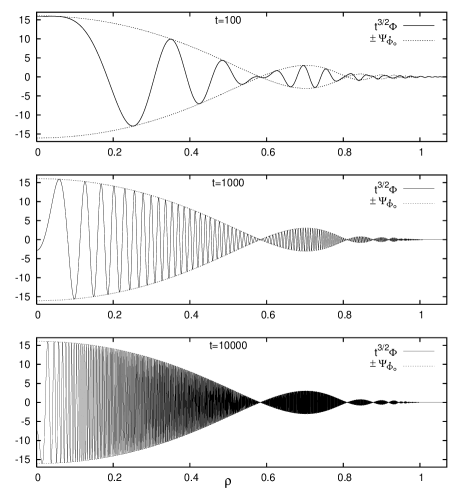
Figure 1: The time evolution of a KG field with initial data $\Phi|_{\Sigma_{0}}=0$ and $(\partial_{t}\Phi)|_{\Sigma_{0}}=\dot{\Phi}_{\circ}$ is shown. In order to compensate the fast expansion and the decay in time, instead of the field amplitude $\Phi$ the combination $t^{3/2}\Phi$ is plotted on the three successive time slices $t=100$, $t=1000$, and $t=10000$ against the variable $\rho=\frac{r}{t}$. Notice that the value $\rho=1$ labels the point sitting at the light cone emanating from the center at $t=0$. The graphs $\pm\Psi_{\dot{\Phi}_{\circ}}$ – for the definition of $\Psi_{\dot{\Phi}_{\circ}}$ see (III.17) and (LABEL:f11) – are also shown by the dashed curves. On the early time slice $t=100$ the final segment does not fit the contours $\pm\Psi_{\dot{\Phi}_{\circ}}$; however, at later times where conditions III.1 and III.2 are satisfied in larger and larger portions of the time slices, the exact oscillations get closer and closer to the contours.

Figure 2: The final segments of the plots of Fig. 1 for $\rho>0.9$ on the time slices $t=1000$ and $t=10000$. It is remarkable to what extent the high frequency oscillations fit to the contours $\pm\Psi_{\dot{\Phi}_{\circ}}$ even in the region far away from the origin on the time slice $t=10000$.

Next, we describe a method based on an approximation which explains the appearance of these stable structures and provides a quantitative account of the underlying phenomenon to a high precision. It is surprising by itself that under the conditions introduced below the integrand of Eq. (III.2) can be very precisely approximated by a function so that the integral (III.2) takes a very simple form.

We denote by $\bar{r}^{\prime}$ the radius of the smallest sphere $\mathcal{B}(O,\bar{r}^{\prime})$ centered at the origin so that $\mathcal{B}(O,\bar{r}^{\prime})$ contains the compact support of the specified initial data on $\Sigma_{0}$.

Condition III.1

: We shall say that a point $p$, with coordinates $(t,r)$, of the time slice $\Sigma_{t}$ is in the region of the approximation if for a given $\epsilon<1$ the relation

$$\bar{r}^{\prime}<\epsilon(t-r)$$ (III.6)

holds.

Notice that on a fixed time slice the smaller the value of $\epsilon$ the more precise the approximated field value, although the domain of the approximation gets smaller. The numerical results indicate that even for the relatively large $\epsilon=1/10$ there is surprisingly good agreement between the exact and approximated field values. For an arbitrarily small fixed value of $\epsilon$ the domain where the approximation breaks down is $t-\bar{r}^{\prime}/\epsilon<r<t+r^{\prime}$. The size of this region, independently of time, is $\bar{r}^{\prime}(1+1/\epsilon)$, while the domain of the approximation $0\leq t-\bar{r}^{\prime}/\epsilon$ grows linearly with $t$. Thereby one may think of condition III.1 as holding asymptotically almost everywhere inside the causal future of the compact support of the initial data.

In the domain where condition III.1 holds, both $\lambda_{0}$ and $\lambda_{\pi}$ are positive, so then $H(\lambda_{0})=H(\lambda_{\pi})=1$. In addition, we have that

$$\frac{r^{\prime}r}{t^{2}-r^{2}}=\frac{r^{\prime}r}{(t-r)(t+r)}<\frac{r^{\prime}}{(t-r)}<\epsilon$$ (III.7)

and similarly

$$\frac{r^{\prime 2}}{t^{2}-r^{2}}<\frac{r^{\prime}}{(t-r)}\frac{r^{\prime}}{t}<\epsilon.$$ (III.8)

Then, by making use of these relations, along with the notation

$$l_{0}=\sqrt{t^{2}-r^{2}},$$ (III.9)

$\sqrt{\lambda_{0}}$ and $\sqrt{\lambda_{\pi}}$ can be approximated as

$$\sqrt{\lambda_{0}} \approx l_{0}\left(1+\frac{r^{\prime}r}{l_{0}^{2}}-\frac{r^{\prime 2}}{2l_{0}^{2}}\right),$$ (III.10)

$$\sqrt{\lambda_{\pi}} \approx l_{0}\left(1-\frac{r^{\prime}r}{l_{0}^{2}}-\frac{r^{\prime 2}}{2l_{0}^{2}}\right).$$ (III.11)

Moreover, for $z\gg 1$ the Bessel function $J_{0}(z)$ can also be very closely approximated as

$$J_{0}(z)\approx\sqrt{\frac{2}{\pi z}}\sin\left(z+\frac{\pi}{4}\right).$$ (III.12)

By virtue of Eqs. (III.10) and (III.11), whenever condition III.1 holds, both the arguments of $J_{0}$ in Eq. (III.2), i.e., $m\sqrt{\lambda_{0}}$ and $m\sqrt{\lambda_{\pi}}$, are much greater than $1$ provided that the following condition holds.

Condition III.2

: The condition

$$ml_{0}\gg 1$$ (III.13)

is satisfied.

This condition certainly holds in the region of approximation of condition III.1 if $t$ is chosen to be sufficiently large, i.e., for $t\gg\frac{1}{m}$.

For large values of $z$ the function $\sqrt{\frac{2}{\pi z}}\sin\left(z+\frac{\pi}{4}\right)$ has a high frequency oscillation with a negligible change in the amplitude. Therefore we shall further simplify the approximation (III.12) of $J_{0}(z)$ applied for the arguments $z=m\sqrt{\lambda_{0}}$ and $z=m\sqrt{\lambda_{\pi}}$ as

$$J_{0}(z)\approx\sqrt{\frac{2}{m\pi l_{0}}}\sin\left(z+\frac{\pi}{4}\right).$$ (III.14)

Hence, whenever conditions III.1 and III.2 are satisfied, the substitution of Eq. (III.14) into Eq. (III.2) yields

$$\Phi(t,r)\approx\frac{1}{2r}\sqrt{\frac{2}{\pi m\,l_{0}}}\int\limits_{0}^{\infty}r^{\prime}\dot{\Phi}_{\circ}(r^{\prime})$$

$$\hskip 14.22636pt\cdot\left[\sin\left(m\sqrt{\lambda_{0}}+\frac{\pi}{4}\right)-\sin\left(m\sqrt{\lambda_{\pi}}+\frac{\pi}{4}\right)\right]dr^{\prime}.$$

Then by making use of Eqs. (III.10), (III.11) and keeping the leading order term, a straightforward calculation results in

$$\Phi(t,r)\approx\frac{1}{r}\sqrt{\frac{2}{\pi m\,l_{0}}}\cos\left(ml_{0}+\frac{\pi}{4}\right)$$

$$\hskip 25.6073pt\cdot\int\limits_{0}^{\infty}r^{\prime}\dot{\Phi}_{\circ}(r^{\prime})\sin\left(\frac{mr}{l_{0}}r^{\prime}\right)dr^{\prime}.$$ (III.16)

Finally, by introducing $\rho=\frac{r}{t}$, the self-similarity variable, Eq. (III.16) can be recast into the form

$$\Phi(t,r)\approx{t^{-\frac{3}{2}}}\Psi_{\dot{\Phi}_{\circ}}(\rho)\cos\left(m\sqrt{t^{2}-r^{2}}+\frac{\pi}{4}\right),$$ (III.17)

where

$$\Psi_{\dot{\Phi}_{\circ}}(\rho) = \sqrt{\frac{2}{m\pi}}\rho^{-1}(1-\rho^{2})^{-\frac{1}{4}}$$

$$\cdot\int\limits_{0}^{\infty}r^{\prime}\dot{\Phi}_{\circ}(r^{\prime})\sin\left(\frac{m\rho r^{\prime}}{\sqrt{1-\rho^{2}}}\right)dr^{\prime}.$$

Notice that the integral term of Eq. (LABEL:f11) is, in fact, the real part of the Fourier transform of the function $r\dot{\Phi}_{\circ}(r)$. The cosine term of Eq. (III.17) gives a high frequency oscillation that is completely independent of the specified initial data function, i.e., of $\dot{\Phi}_{\circ}(r)$. The amplitude of this high frequency oscillation is modulated by the rest of the expression. There is an overall factor $t^{-3/2}$ scaling down the modulation in time. However, the term $\Psi_{\dot{\Phi}_{\circ}}(\rho)$ depends on $t$ and $r$ only in the combination $\rho={r}/{t}$, so this term represents the self-similar outward expansion of the modulation.

For simple polynomial choices of the initial data function $\dot{\Phi}_{\circ}$, the explicit form of $\Psi_{\dot{\Phi}_{\circ}}(\rho)$ can always be determined. In particular, for a centered step function, i.e., with $\dot{\Phi}_{\circ}$ taking the value $c\in\mathbb{R}^{+}$ for $0\leq r\leq r_{b}$ and being zero elsewhere,

$$\Psi_{\dot{\Phi}_{\circ}}(\rho) = c\sqrt{\frac{2}{m\pi}}\frac{(1-\rho^{2})^{\frac{3}{4}}}{m^{2}\rho^{3}}$$

$$\cdot\left[\sin\left(\frac{mr_{b}\rho}{\sqrt{1-\rho^{2}}}\right)-\frac{mr_{b}\rho}{\sqrt{1-\rho^{2}}}\cos\left(\frac{mr_{b}\rho}{\sqrt{1-\rho^{2}}}\right)\right].$$

It is remarkable to what extent the high frequency oscillations fit the contours $\pm\Psi_{\dot{\Phi}_{\circ}}$ (see Figs. 1 and 2). We would like to emphasize, however, that not only this overall behavior can be described properly by the approximation method outlined above. Figure $3$ shows the exact field value $\Phi$, along with its approximated value $\Phi_{a}$, where the values of $\Phi$ and $\Phi_{a}$ are determined by making use of the relations (III.2) and (III.17), respectively. Since there is an almost exact coincidence between the two relevant curves, only the final segment with $\rho>0.93$ is shown in Fig. 3 for the time slice $t=1000$.

Figure 3: The exact value field value $\Phi$ along with its value $\Phi_{a}$ as it is approximated by the relation (III.17) are shown for $\rho>0.93$ and for the time slice $t=1000$.

We would like to emphasize that for a fixed radius $r$ and for large enough values of $t$ we have that $\Psi_{\dot{\Phi}_{\circ}}(\rho)\approx\Psi_{\dot{\Phi}_{\circ}}(0)=\sqrt{\frac{2m}{\pi}}\int\limits_{0}^{\infty}{r^{\prime}}^{2}\dot{\Phi}_{\circ}(r^{\prime})dr^{\prime}$ and $l_{0}\approx t$, so that for a scalar monopole Eq. (III.17) restores the inverse power-law behavior of Eq. (I.1) relevant for $l=0$.

One might have the impression that the apparent increase of the maximal frequency of the oscillations on the above figures is merely a coordinate effect, i.e., it is a simple consequence of the use of the self-similarity variable $\rho=r/t$, and one might suspect that it will not occur if the plots are made against the radial coordinate $r$. Nevertheless, the following graphs (see Fig. 4) show that the increase of the maximal frequency along the $t=const.$ slices is a true physical effect.

Figure 4: Equal length ($\Delta r=60$) final segments of the true (nonapproximated) oscillations of $t^{-3/2}\Phi$ are shown at the time slices $t=1000$, $t=10000$, and $t=100000$. The associated graphs demonstrate that the increase of the maximal frequency of the oscillations does really occur, even though the plots are made against the $r$ coordinate representing real physical distances.

A simple explanation of this phenomenon can be given based on the use of the approximation (III.17) as follows. Since the term responsible for the high frequency oscillations is $\cos(ml_{0}(t,r)+\pi/4)$ the frequencies $\omega_{t}$ and $\omega_{r}$ – relevant for the $r=const.$ lines and for the $t=const.$ hypersurfaces – can be read off from the approximation of the term $ml_{0}$ in the neighborhood of a point with coordinates $(t,r)$ as

$$\hskip-11.38092ptml_{0}(t+\Delta t,r+\Delta r)\approx ml_{0}(t,r)+\omega_{t}\Delta t-\omega_{r}\Delta r,$$ (III.20)

where the frequencies are

$$\omega_{t} = m\partial_{t}l_{0}=m\frac{t}{\sqrt{{t}^{2}-{r}^{2}}},$$ (III.21)

$$\omega_{r} = -m\partial_{r}l_{0}=m\frac{r}{\sqrt{{t}^{2}-{r}^{2}}},$$ (III.22)

respectively. It follows from these expressions that as $r$ tends to the value of $t$ both $\omega_{t}$ and $\omega_{r}$ grow without any upper bound, although their ratio tends to $1$. This, in particular, implies that the self-similar part of the modulation expands (at least at the “outer edge”) with the velocity of light. The frequency of the oscillation at a fixed distance $\Delta r=t-r$ from the “outer edge” ($t=r$) grows as $\sqrt{t}$, as it can be seen from the approximation

$$\omega_{r}\approx\omega_{t}=\frac{t}{\sqrt{\Delta r}\sqrt{t+r}}\approx\frac{1}{\sqrt{2\Delta r}}\sqrt{t}$$ (III.23)

relevant for $\Delta r\ll t$. This, in turn, implies – in accordance with Fig. 4 – that more and more oscillations will be associated with the final segments of length $\Delta r$ as the time increases.

It is also informative to consider what can be seen by a static observer, moving along an $r=const.$ world-line with $r\gg\bar{r}^{\prime}$. First, a very high frequency oscillation arrives at $t=r-\bar{r}^{\prime}$ with amplitude growing gradually from zero. In the domain where the approximation (III.17) is valid, the amplitude of this oscillation becomes modulated by ${t^{-\frac{3}{2}}}\Psi_{\dot{\Phi}_{\circ}}(\rho)$, while $\rho=r/t$ decreases from a value close to $1$ to $0$. By virtue of Eq. (III.21) the frequency of the high frequency oscillation gradually decreases, settling down finally to the value $\omega_{t}=m$ in accordance with Eq. (I.1).

IV Evolution of a temporarily static configuration

Start now with a static initial data function, i.e., assume that $(\partial_{t}\Phi)|_{\Sigma_{0}}=0$ and $\Phi|_{\Sigma_{0}}=\Phi_{\circ}(r)$ where $\Phi_{\circ}:[0,\infty)\rightarrow\mathbb{R}$ is a sufficiently regular function of $r$ with compact support. Now to get the associated field values we have to evaluate only the second term of Eq. (II.5). In particular, at a point of the axis of rotation with coordinates $x^{\alpha}=(t,r,0,0)$, with $t>0$, we obtain from Eq. (II.5)

$$\Phi(t,r) = -\int\limits_{0}^{\infty}dr^{\prime}\int\limits_{0}^{\pi}d\vartheta^{\prime}\int\limits_{0}^{2\pi}d\varphi^{\prime}$$ (IV.1)

$$\cdot\Phi_{\circ}(r^{\prime})\left[\frac{\partial}{\partial{t^{\prime}}}G(t,r;t^{\prime},r^{\prime},\varphi^{\prime},\vartheta^{\prime})\right]_{t^{\prime}=0}{r^{\prime}}^{2}\sin\vartheta^{\prime}$$

$$= -\frac{t}{r}\int\limits_{0}^{\infty}dr^{\prime}r^{\prime}\Phi_{\circ}(r^{\prime})\int\limits_{0}^{\pi}d\vartheta^{\prime}$$

$$\cdot\frac{\partial}{\partial\vartheta^{\prime}}\left[\delta(\lambda)-\frac{m}{2\sqrt{\lambda}}H(\lambda)J_{1}(m\sqrt{\lambda})\right],$$

where the relation

$$\frac{\partial}{\partial{t^{\prime}}}=\frac{\partial\lambda}{\partial{t^{\prime}}}\left(\frac{\partial\lambda}{\partial{\vartheta^{\prime}}}\right)^{-1}\frac{\partial}{\partial{\vartheta^{\prime}}}=\frac{t-t^{\prime}}{r^{\prime}r\sin\vartheta^{\prime}}\frac{\partial}{\partial{\vartheta^{\prime}}},$$ (IV.2)

along with Eq. (II.2), has also been used. By evaluating the $\vartheta^{\prime}$ integral of Eq. (IV.1) we get

$$\Phi(t,r)=\frac{t}{r}\int\limits_{0}^{\infty}dr^{\prime}\ r^{\prime}{\Phi}_{\circ}(r^{\prime})\bigg{[}\delta(\lambda_{0})-\delta(\lambda_{\pi})\bigg{.}$$

$$\bigg{.}-\frac{m}{2}\left(\frac{H(\lambda_{0})}{\sqrt{\lambda_{0}}}J_{1}(m\sqrt{\lambda_{0}})-\frac{H(\lambda_{\pi})}{\sqrt{\lambda_{\pi}}}J_{1}(m\sqrt{\lambda_{\pi}})\right)\bigg{]}.$$

(IV.3)

For determination of the parts of the above integral containing the Dirac delta terms we used the relations

$$\int\limits_{0}^{\infty}\delta(\lambda_{0})\psi(r^{\prime})dr^{\prime} = \int\limits_{0}^{r}\delta(\lambda_{0})\psi(r^{\prime})dr^{\prime}+\int\limits_{r}^{\infty}\delta(\lambda_{0})\psi(r^{\prime})dr^{\prime}$$ (IV.4)

$$= \int\limits_{t^{2}-r^{2}}^{t^{2}}\delta(\lambda_{0})\psi(r^{\prime})(\partial_{r^{\prime}}\lambda_{0})^{-1}d\lambda_{0}$$

$$+ \int\limits_{t^{2}}^{-\infty}\delta(\lambda_{0})\psi(r^{\prime})(\partial_{r^{\prime}}\lambda_{0})^{-1}d\lambda_{0}$$

$$=\frac{1}{2}H(r-t)\left(\frac{\psi(r^{\prime})}{r-r^{\prime}}\right)_{r^{\prime}=r-t}-\frac{1}{2}\left(\frac{\psi(r^{\prime})}{r-r^{\prime}}\right)_{r^{\prime}=r+t}$$

$$=\frac{1}{2t}\big{[}\psi(r+t)+H(r-t)\psi(r-t)\big{]},$$

and

$$\int\limits_{0}^{\infty}\delta(\lambda_{\pi})\psi(r^{\prime})dr^{\prime} = \frac{1}{2}H(t-r)\left(\frac{\psi(r^{\prime})}{r^{\prime}+r}\right)_{r^{\prime}=t-r}$$

$$= \frac{1}{2t}H(t-r)\psi(t-r),$$ (IV.5)

where $\psi:[0,\infty)\rightarrow\mathbb{R}$ is considered to be a sufficiently regular but otherwise arbitrary function. Thereby, we get from Eq. (IV.3)

$$\Phi(t,r)=-\frac{mt}{2r}\int\limits_{0}^{\infty}r^{\prime}\Phi_{\circ}(r^{\prime})$$

$$\cdot\left[\frac{H(\lambda_{0})}{\sqrt{\lambda_{0}}}J_{1}(m\sqrt{\lambda_{0}})-\frac{H(\lambda_{\pi})}{\sqrt{\lambda_{\pi}}}J_{1}(m\sqrt{\lambda_{\pi}})\right]dr^{\prime}$$

$$\hskip 17.07182pt+\frac{1}{2r}\big{[}(r+t)\Phi_{\circ}(r+t)+(r-t)\Phi_{\circ}(|r-t|)\big{]}.$$

(IV.6)

This integral has been evaluated numerically and the relevant plots on the time slices $t=500$ and $t=5000$ are shown in Figs. 5 and 6. Here the initial data function was chosen to possess the analytic form of (III.5), i.e., $\Phi_{\circ}=f(r)$, with parameters $a=0$, $b=5$, $c=1$ and $d=15$ corresponding to a bell shaped initial configuration centered at the origin with radius $r=5$.

Figure 5: The time evolution of a KG field with initial data function $\Phi|_{\Sigma_{0}}=\Phi_{\circ}$ and $(\partial_{t}\Phi)|_{\Sigma_{0}}=0$ is plotted at the two successive time slices $t=500$ and $t=5000$ against the variable $\rho=\frac{r}{t}$. The graphs $\pm\Psi_{\Phi_{\circ}}$ – for the definition of $\Psi_{\Phi_{\circ}}$ see Eqs. (IV.8) and (IV.9) – are also indicated by the dashed curves.

Figure 6: The final segment of the second plot of Fig. 5 restricted to $\rho>0.9$ together with an even smaller portion relevant for a later time slice $t=50000$ with $\rho>0.995$ are shown.

In the domain where conditions III.1 and III.2 are valid, in particular, whenever $t$ is sufficiently large, the nonintegral terms of Eq. (IV.6) are zero, since both $r+t$ and $|r-t|$ are larger than the radius $\bar{r}^{\prime}$ of the initial data function. Furthermore, the integral term in Eq. (IV.6) can be approximated by exactly the same procedure as that used in case of Eq. (III.2). To see this, note first that for $z\gg 1$ the Bessel function $J_{1}(z)$ can be very closely approximated as

$$J_{1}(z)\approx-\sqrt{\frac{2}{\pi z}}\cos\left(z+\frac{\pi}{4}\right).$$ (IV.7)

Then, in particular, whenever conditions III.1 and III.2 are satisfied by making use of Eqs. (III.10) and (III.11), along with the self-similarity variable $\rho=\frac{r}{t}$, the integral term, and thereby $\Phi(t,r)$ itself, can be approximated as

$$\Phi(t,r)\approx{t^{-\frac{3}{2}}}\Psi_{\Phi_{\circ}}(\rho)\sin\left(m\sqrt{t^{2}-r^{2}}+\frac{\pi}{4}\right),$$ (IV.8)

where

$$\Psi_{\Phi_{\circ}}(\rho)=-\sqrt{\frac{2m}{\pi}}\rho^{-1}(1-\rho^{2})^{-\frac{3}{4}}$$

$$\hskip 51.21504pt\cdot\int\limits_{0}^{\infty}r^{\prime}\Phi_{\circ}(r^{\prime})\sin\left(\frac{m\rho r^{\prime}}{\sqrt{1-\rho^{2}}}\right)dr^{\prime}.$$

(IV.9)

Notice that Eq. (IV.8) has the same type of structure as Eq. (III.17). The sine term of Eq. (IV.8) again represents a high frequency oscillation that is completely independent of the specified initial data. The amplitude of this high frequency oscillation is modulated by the overall factor $t^{-3/2}$, scaling down the modulation in time, along with $\Psi_{\Phi_{\circ}}$. Again the term $\Psi_{\Phi_{\circ}}$ depends on $t$ and $r$ only via the combination $\rho={r}/{t}$ and as in the case of Eq. (III.17) this term gives a self-similar outward expansion of the modulation.

V The appearance of the shells in terms of the energy density

As is obvious from the relations (II.8) and (II.9), to be able to evaluate the energy density and the energy current density expressions in addition to Eqs. (III.2) and (IV.6) we also need to determine the derivatives of the field variable $\Phi$ with respect to $t$ and $r$, respectively. These derivatives, by straightforward calculation, although a bit more involved than the previous ones, for a generic initial data $\Phi|_{\Sigma_{0}}=\Phi_{\circ}(r)$ and $(\partial_{t}\Phi)|_{\Sigma_{0}}=\dot{\Phi}_{\circ}(r)$ can be shown to take the form

$$\partial_{t}\Phi(t,r) = \frac{1}{t}\Phi(t,r)-\frac{mt}{2r}\int\limits_{0}^{\infty}r^{\prime}\dot{\Phi}_{\circ}(r^{\prime})\left[\frac{H(\lambda_{0})}{\sqrt{\lambda_{0}}}J_{1}(m\sqrt{\lambda_{0}})-\frac{H(\lambda_{\pi})}{\sqrt{\lambda_{\pi}}}J_{1}(m\sqrt{\lambda_{\pi}})\right]dr^{\prime}$$ (V.1)

$$\hskip 31.2982pt+\frac{m^{2}t^{2}}{2r}\int\limits_{0}^{\infty}r^{\prime}\Phi_{\circ}(r^{\prime})\left[\frac{H(\lambda_{0})}{\lambda_{0}}J_{2}(m\sqrt{\lambda_{0}})-\frac{H(\lambda_{\pi})}{\lambda_{\pi}}J_{2}(m\sqrt{\lambda_{\pi}})\right]dr^{\prime}$$

$$+\frac{1}{2r}\big{[}(r+t)\dot{\Phi}_{\circ}(r+t)+(r-t)\dot{\Phi}_{\circ}(|r-t|)+(r+t)\Phi_{\circ}^{\prime}(r+t)-|r-t|\Phi_{\circ}^{\prime}(|r-t|)\big{]}$$

$$-\frac{1}{2t}\big{[}\Phi_{\circ}(r+t)-\Phi_{\circ}(|r-t|)\big{]}-\frac{m^{2}t}{4r}\big{[}(r+t)\Phi_{\circ}(r+t)+(r-t)\Phi_{\circ}(|r-t|)\big{]}$$

and

$$\partial_{r}\Phi(t,r) = +\frac{m}{2r}\int\limits_{0}^{\infty}r^{\prime}\dot{\Phi}_{\circ}(r^{\prime})\left[\frac{H(\lambda_{0})(r-r^{\prime})}{\sqrt{\lambda_{0}}}J_{1}(m\sqrt{\lambda_{0}})-\frac{H(\lambda_{\pi})(r+r^{\prime})}{\sqrt{\lambda_{\pi}}}J_{1}(m\sqrt{\lambda_{\pi}})\right]dr^{\prime}$$

$$-\frac{m^{2}t}{2r}\int\limits_{0}^{\infty}r^{\prime}\Phi_{\circ}(r^{\prime})\left[\frac{H(\lambda_{0})(r-r^{\prime})}{\lambda_{0}}J_{2}(m\sqrt{\lambda_{0}})-\frac{H(\lambda_{\pi})(r+r^{\prime})}{\lambda_{\pi}}J_{2}(m\sqrt{\lambda_{\pi}})\right]dr^{\prime}$$

$$-\frac{m^{2}t}{4r}\big{[}(r+t)\Phi_{\circ}(r+t)-(r-t)\Phi_{\circ}(|r-t|)\big{]}+\frac{1}{2r}\big{[}(r+t)\dot{\Phi}_{\circ}(r+t)-(r-t)\dot{\Phi}_{\circ}(|r-t|)\big{.}$$

$$\big{.}+\Phi_{\circ}(r+t)+(r+t)\Phi_{\circ}^{\prime}(r+t)+\Phi_{\circ}(|r-t|)+|r-t|\Phi_{\circ}^{\prime}(|r-t|)\big{]}-\frac{1}{r}\Phi(t,r),$$

where $\Phi_{\circ}^{\prime}$ stands for the $r$ derivative of the function $\Phi_{\circ}(r)$. Then by making use of Eqs. (II.8) and (II.9), along with Eqs. (III.2), (IV.6), (V.1), and (LABEL:drPhiv), we can evaluate the energy density and energy current density expressions. For the choice of initial data function used in Sec. III to produce Figs. 1 and 2, the various plots of the energy density on the time level surfaces $t=100$, $t=1000$, and $t=10000$ are shown in Figs. 7 and 8.

Figure 7: The energy density profile relevant for the excitation of the initially vacuum configuration of Sec. III, is shown for the time slices $t=100$, $t=1000$ and $t=10000$.

Figure 8: The final segments of the energy density profile of Fig. 7 is shown for $\rho>0.9$ and for the time slices $t=1000$ and $t=10000$.

The corresponding energy current density profile on the time level surfaces $t=100$, $t=1000$ and $t=10000$ is shown in Fig. 9.

Figure 9: The energy current density profile relevant for the excitation of the initially vacuum configuration of Sec. III is shown for the time slices $t=100$, $t=1000$, and $t=10000$.

Similarly, for the choice of initial data function used in Sec. IV to produce Figs. 5 and 6, the various plots of the energy density on the time level surfaces $t=500$, $t=5000$, and $t=50000$ are shown in Figs. 10 and 11.

Figure 10: The energy density profile relevant for the excitation of the initially static configuration of Sec. IV, is shown for the time slices $t=500$ and $t=5000$.

Figure 11: Two different final segments of the energy density profile of Fig. 10 are shown for the time slice $t=5000$ with $\rho>0.9$ and for the time slice $t=50000$ with $\rho>0.995$.

In order to represent more clearly the ratio of the total energy carried by individual shells in the spherically symmetric configuration investigated, instead of the energy density $\varepsilon$ and the energy current density $S$, we plotted the quantities $4\pi r^{2}\varepsilon$ and $4\pi r^{2}S$ representing the energy and energy current in thin spherical shells. Since we are using $\rho=r/t$ as a radial coordinate on our plots we also have to multiply these values by $\frac{dr}{d\rho}=t$

$$E=\int_{0}^{t+\bar{r}^{\prime}}4\pi r^{2}\varepsilon dr=\int_{0}^{1+\frac{\bar{r}^{\prime}}{t}}4\pi r^{2}t\varepsilon d\rho,$$ (V.3)

in order to be able to estimate the energy as the area under the plotted curves.

Notice that the formation of self-similarly expanding shells is manifested strikingly by Figs. 7 - 11 in spite of the fact that no approximation has been used anywhere in the associated calculations.

VI Concluding remarks

In this paper the time evolution of initially concentrated spherically symmetric massive KG fields has been investigated. By means of concrete examples and by a suitable approximation method the following characteristic properties have been found. There is an overall high frequency oscillation of the field value which is modulated by two factors. First, there is a time decaying factor of the form $t^{-3/2}$ consistent with the total energy conservation. Second, the field amplitude is also modulated by a self-similar contour, i.e., apart from the scaling down $t^{-3/2}$ the oscillations expand essentially self-similarly. The associated self-similar contours were found to possess knots, whereby the oscillations are separated into individual shells. Since the overall exponent of the scaling down factor is independent of the radial coordinate, the fraction of the energy carried by an individual expanding shell is also preserved during the entire evolution. The exact form of the shells, which is approximated to higher and higher precision in larger and larger domains of the associated domain of dependence, is determined essentially by the Fourier transform of the initial data.

It is of obvious interest to know whether the results presented in this paper have any relevance for initial data with noncompact support. To be able to answer this question it is necessary to check whether the conditions applied throughout our analysis, i.e., conditions III.1 and III.2, can be satisfied at least in a generalized sense. We have investigated this issue briefly and we found the following. Suppose that we have a non-compact support initial data function, which, however, is focused sufficiently on the central region, i.e., it decays rapidly. Then we can associate a finite characteristic size with the support of such an initial data function. We expect that condition III.1 can be replaced by the requirement that this characteristic size should be small compared to $\epsilon(t-r)$. If we have an initial data function of this type and, in addition, condition III.2 holds, basically the same type of approximations and plots can be produced for the field values and for the energy densities as was possible in the case of initial data with compact support. It might be interesting that for initial data functions $\Phi|_{\Sigma_{0}}=\Phi_{\circ}(r)$ and $(\partial_{t}\Phi)|_{\Sigma_{0}}=0$, where $\Phi_{\circ}(r)$ was chosen to possess the form $\Phi_{\circ}(r)=\exp(-r^{2}/d)$ (with $d\in\mathbb{R}^{+}$), there was no knot on the the associated contours $\pm\Psi_{\Phi_{\circ}}$, while for the choice $\Phi_{\circ}(r)={d}/{(d+r^{8})}$ (with $d\in\mathbb{R}^{+}$) the very same type of figures, with shells and oscillations, were obtained as in the case of initial data with compact support. Investigation of more general initial data specifications with noncompact support, as well as a careful adaptation of the approximation procedure applied throughout this paper, deserves further attention.

It would also be important to know to what extent the results presented in this paper may have relevance in more complicated physical situations, for instance, in the case of nonlinear self-interacting fields, or whenever instead of the Minkowski spacetime the evolution is investigated on a general asymptotically flat background spacetime. Note, however, that in the asymptotic region the field equation relevant for a self-interacting possibly nonlinear scalar field in many cases is expected to reduce to the equation of a massive KG field; moreover, in that region the geometry also tends to the form of the Minkowski metric. Thereby it seems to be plausible to assume that the formation of shell structures, as well as the time decay rate and the self-similar behavior of the modulation, will probably occur in any asymptotically flat spacetime (regardless of whether the geometry is dynamical or not) and for any massive field that can be approximated by a massive KG field in the asymptotic region.

References

- (1) L.M. Burko and A. Ori: Late-time evolution of nonlinear gravitational collapse, Phys. Rev. D 56, 7820-7832 (1997)
- (2) C. Gundlach , R. H. Price and J. Pullin: Late-time behavior of stellar collapse and explosion. I. Linearized perturbations, Phys. Rev. D 49, 883-889 (1994)
- (3) C. Gundlach, R. H. Price and J. Pullin: Late-time behavior of stellar collapse and explosion. II. Nonlinear evolution, Phys. Rev. D 49, 890-899 (1994)
- (4) E.W. Leaver: Spectral decomposition of the perturbation response of the Schwarzschild geometry, Phys. Rev. D 34, 384-408 (1986)
- (5) R. H. Price: Non-spherical perturbation of relativistic gravitational collapse. I. Scalar and gravitational perturbations, Phys. Rev. D 5, 2419-2438 (1972)
- (6) E.P. Honda and M. W. Choptuik: Fine Structure of Oscillons in the Spherically Symmetric Klein-Gordon Model, Phys. Rev. D 65, 084037 (2002)
- (7) S. Hod and T. Piran: Late-time tails in gravitational collapse of a self-interacting (massive) scalar-field and decay of a self-interacting scalar hair, Phys. Rev. D 58, 044018 (1998)
- (8) H. Koyama and A. Tomimatsu: Slowly decaying tails of massive scalar fields in spherically symmetric spacetimes, Phys. Rev. D 65, 084031 (2002)
- (9) F. Pretorius and L. Lehner: Adaptive Mesh Refinement for Characteristic Codes, gr-qc/0302003 (2003)
- (10) J. Winicour: Massive fields at null infinity, J. Math. Phys. 29, 2117-2121 (1988)
- (11) G. Fodor and I. Rácz: On the Time Evolution of Magnetic Monopoles, in preparation
- (12) GNU Scientific Library, http://www.gnu.org/software/gsl/