hep-th/0308117
AEI 2003-068

1 Introduction

It is believed that free type IIB superstring theory on the $AdS_{5}\times S^{5}$ background is exactly dual to planar ${\cal N}=4$ supersymmetric $SU(N)$ quantum gauge theory [1, 2, 3]. Here

$$4\pi g_{s}=\frac{\lambda}{N}=0\quad\mbox{for}\quad N=\infty\ ,\ \ \ \ \ \ \lambda=Ng_{\scriptscriptstyle\mathrm{YM}}^{2}={\rm fixed}\ ,$$ (1.1)

and $\lambda$ is the ’t Hooft coupling constant. Since the exact quantization of string theory in this curved background is not yet understood, most of the results on the string side of the duality obtained until a year and a half ago were in the (classical) supergravity limit of infinite string tension ${\frac{1}{2\pi\alpha^{\prime}}}\rightarrow\infty$, which corresponds, via the “effective string tension” identification

$$\sqrt{\lambda}=\frac{R^{2}}{\alpha^{\prime}}\ ,$$ (1.2)

to the strong coupling limit on the planar gauge theory side. Since in string theory little could be done at finite $\alpha^{\prime}$ and $R$, while in gauge theory little could be done at finite $\lambda$, until recently the perception was that any dynamical test of the AdS/CFT correspondence should be very hard to perform. A notable exception were some successful studies of four-point functions (involving BPS operators on the gauge side and supergravity correlators on the string side) where some dynamical modes appear in intermediate channels [4, 5, 6]. This situation has dramatically improved due to new ideas and techniques on both sides of the correspondence, which were largely influenced by the seminal work of [7] (which, in turn, was based on [8, 9]). Very recent progress points towards the exciting prospect that the free $AdS_{5}\times S^{5}$ string alias planar gauge theory is integrable and thus might be exactly solvable.

On the string theory side, it was understood that in the case when some of the quantum numbers of the string states become large, the $AdS_{5}\times S^{5}$ string sigma model can be efficiently treated by semi-classical methods [10, 11] (see also [12] and [13, 14, 15]). It was then suggested [16, 17] that a novel possibility for a quantitative comparison with SYM theory in non-BPS sectors appears when one considers classical solutions describing closed strings rotating in several directions in the product space $AdS_{5}\times S^{5}$ with the metric $ds^{2}_{10}=(ds^{2})_{AdS_{5}}+(ds^{2})_{S^{5}}$

$$(ds^{2})_{AdS_{5}}\mathrel{} = \mathrel{}d\rho^{2}-\cosh^{2}\rho\ dt^{2}+\sinh^{2}\rho\ (d\theta^{2}+\cos^{2}\theta\ d\phi^{2}_{1}+\sin^{2}\theta\ d\phi_{2}^{2})$$

$$(ds^{2})_{S^{5}}\mathrel{} = \mathrel{}d\gamma^{2}+\cos^{2}\gamma\ d\varphi_{3}^{2}+\sin^{2}\gamma\ (d\psi^{2}+\cos^{2}\psi\ d\varphi_{1}^{2}+\sin^{2}\psi\ d\varphi_{2}^{2})$$ (1.3)

Here $t$ is the global $AdS_{5}$ time, which, together with the 5 angles $(\phi_{1},\phi_{2};\varphi_{1},\varphi_{2},\varphi_{3})$, correspond to the obvious “linear” isometries of the metric, i.e. are related to the 3+3 Cartan generators of the $SO(2,4)\times SO(6)$ bosonic isometry group. Rotating strings can thus carry the 2+3 angular momentum charges (spins) $Q_{i}=(S_{1},S_{2};J_{1},J_{2},J_{3})$, while $t$ is associated with the energy $E$. Once such classical solutions representing string states with several charges are found [11, 16, 17, 18, 19], one may evaluate the energy as a function of the spins and $\lambda$: $E=E(Q_{i},\lambda)$. A remarkable feature of string solutions in $AdS_{5}$ is that their energy grows, for large charges, linearly with the charges [20, 10, 11]. Corrections to subleading terms in the classical energy can then be computed using the standard semiclassical (inverse string tension) expansion [11, 17]. For certain string states with large total spin $J=J_{1}+J_{2}+J_{3}$ on $S^{5}$ for which

$$J\gg 1\ ,\qquad\frac{\lambda}{J^{2}}\ll 1\ ,\qquad Q_{i}\sim J\ ,$$ (1.4)

it turns out that string sigma model loop corrections to the energy are suppressed by powers of ${\frac{1}{J}}$ (see [17, 18, 19]). In these cases the leading, $\mathcal{O}(J)$, contribution to the energy is given already by the classical string expression, i.e. one does not even need to quantize the string sigma model. Furthermore, as follows from the string action, classically, all charges (including the energy) appear only in the combination $Q_{i}/\sqrt{\lambda}$. It was shown in [16, 17, 18, 19] that the classical energy $E$ admits an expansion in powers of the small parameter $\lambda/J^{2}$. The upshot of the semiclassical string analysis is then that in the limit (1.4) the string-state energy is given by

$$E(Q_{i},\lambda)=S+J\left(1+\frac{\lambda}{J^{2}}\,\epsilon_{1}(Q_{i}/J)+\frac{\lambda^{2}}{J^{4}}\,\epsilon_{2}(Q_{i}/J)+\ldots\right)+\mathcal{O}(J^{0}),$$ (1.5)

where $\epsilon_{n}(Q_{i}/J)$ are some functions of the spin ratios $Q_{i}/J$, and $\mathcal{O}(J^{0})$ stands for quantum string sigma model corrections.

Considering string states represented by the classical solutions with several charges $(S_{1},S_{2};J_{1},J_{2},J_{3})$ has the added advantage that it helps significantly in identifying the corresponding gauge theory operators. As is well known, ${\cal N}=4$ supersymmetric gauge theory is superconformally invariant, and the bosonic subgroup of the full superconformal group $PSU(2,2|4)$ is $SO(2,4)\times SO(6)$. The energy $E$ of a string state is expected to correspond to the scaling dimension $\Delta$ of the associated conformal operator on the gauge theory side:

$$E(Q_{i},\lambda)_{{\rm string}}=\Delta(Q_{i},\lambda)_{{\rm gauge}}\ .$$ (1.6)

The dimension $\Delta$ is, in general, a non-trivial function of the ’t Hooft coupling $\lambda$. It is not yet known how to compute $\Delta$ exactly, except for supersymmetric BPS operators (for which dimensions are protected, i.e. independent of $\lambda$) and for certain near-BPS operators with large charge $J_{3}$ [7, 21]. In principle, one can compute the dimension $\Delta$ perturbatively at small $\lambda$ as an eigenvalue of the matrix of anomalous dimensions. Obtaining and diagonalizing this matrix is a task where the complexity increases exponentially with the number $L$ of constituent fields. At this point, a comparison to string theory energies may appear almost hopeless, since, on the string side, the total $SO(6)$ charge $J=L$ is required to be large.

Fortunately, it was recently discovered that planar $\mathcal{N}=4$ SYM theory is integrable at the one-loop level [22, 23]. We can therefore make use of the Bethe ansatz for a corresponding spin chain model to obtain directly the eigenvalues of the matrix of anomalous dimensions. This observation proves to be especially useful in the (“thermodynamic”) limit $L\gg 1$, i.e. for a very long spin chain, where the algebraic Bethe equations are approximated by integral equations. For a large number of fields $J=L$, the dimension $\Delta$ appears to have a loop expansion equivalent to the one in (1.5),

$$\Delta(Q_{i},\lambda)=S+J\left(1+\frac{\lambda}{J^{2}}\,\delta_{1}(Q_{i}/J)+\frac{\lambda^{2}}{J^{4}}\,\delta_{2}(Q_{i}/J)+\ldots\right)+\mathcal{O}(J^{0})\,.$$ (1.7)

Again, the coefficients $\delta_{n}$ are functions of the spin ratios $Q_{i}/J$.

The string semiclassical expression (1.5), while formally valid for $\sqrt{\lambda}\gg 1$, is actually exact, since, as was mentioned above, all sigma model corrections are suppressed by $\frac{1}{J}$. Assuming the conditions (1.4) are satisfied, one should be able to compare directly the classical $\mathcal{O}(J)$ term in the string energy (1.5) to the $\mathcal{O}(J)$ scaling dimension in gauge theory (1.7), and to show that

$$\epsilon_{n}(Q_{i}/J)=\delta_{n}(Q_{i}/J).$$ (1.8)

Such a comparison at $\mathcal{O}(\lambda/J^{2})$ order was indeed successfully carried out in [24, 18, 19], where a spectacular agreement between the string theory and gauge theory results for the energy or dimension was found for several two-spin string states represented by circular and folded closed strings rotating in $S^{5}$.

The contents of the present paper is the following. In Section 2 we review the results of the semi-classical computation of the energy of folded strings rotating in two planes on $S^{5}$, the “$(J_{1},J_{2})$” solution [18]. We also review the results of the Bethe ansatz calculations of the anomalous dimensions of the corresponding gauge theory operators [24]. We then present a full analytic proof that in the region of large quantum numbers the relevant terms in the string energy and the gauge operator dimension match, i.e that $\epsilon_{1}$ and $\delta_{1}$ are indeed the same as functions of the spin ratio. This goes beyond the previous “experimental” evidence of matching series expansions. The central part of the present paper is Section 3, where we show that the “$(J_{1},J_{2})$” state represented by the string rotating in two planes in $S^{5}$ can be analytically continued, in both string and gauge theory, to an “$(S,J)$” state represented by a string rotating in just one plane in $S^{5}$, but having also one large spin in $AdS_{5}$ [11]. On the gauge theory side, this requires the use of a recently constructed [23] supersymmetric extension of the above Bethe ansatz. As a result, we find the agreement between the string theory and gauge theory expressions of the energy/dimension also for the “$(S,J)$” solution. In Section 4 we study the possibility to check the matching (1.8) beyond the leading order $n=1$. Using the expression [25] for the gauge theory two-loop dilatation operator, we present numerical evidence that the matching between the string theory and gauge theory results in the case of the $(J_{1},J_{2})$ state extends to at least to the $n=2$ (two-loop) level. Section 5 contains some concluding remarks, The Appendices contain some general remarks and technical details. In particular, in Appendix B we explain the relation between the $(J_{1},J_{2})$ and $(S,J)$ string solutions, and in Appendix C we discuss the solution of the Bethe ansatz system of equations for the spin chain which appeared in Section 3 in connection with the $(S,J)$ case. In Appendix D we compare circular strings on $S^{5}$ with a different “imaginary” solution of the Bethe equations. Finally, in Appendix E we consider the dependence of string energy on the ratio of two spins.

2 Strings rotating on $S^{5}$

Let us start with a discussion of a particular $(J_{1},J_{2})$ state corresponding to a folded string rotating in two planes on the five-sphere. This folded solution should have minimal value of the energy for given values of the spins. Our aim will be to demonstrate the equivalence between the leading correction to the classical string-theory energy and the one-loop gauge theory anomalous dimension at the functional level, i.e. going beyond particular expansions and limits considered previously in [24, 18]. The solution in question [18] has the following non-zero coordinates in (1): $t=\kappa\tau,\ \varphi_{1}={\rm w}_{1}\tau,\ \varphi_{2}={\rm w}_{2}\tau,\ \gamma={\frac{\pi}{2}},\ \psi=\psi(\sigma)$ and $\psi$ satisfies a 1-d sine-Gordon equation in $\sigma$. The string is stretched in $\psi$ with the maximal value $\psi_{0}$ (we refer to Appendices A and B for details on the string solutions). The classical energy and the angular momenta of the rotating string may be written as

$$E=\sqrt{\lambda}\,\mathcal{E},\qquad J_{i}=\sqrt{\lambda}\,\mathcal{J}_{i}.$$ (2.1)

Here and from now on, curly letters correspond to charges rescaled by the inverse effective string tension, $1/\sqrt{\lambda}$. The parameters of the solution $\kappa,\omega_{1},\omega_{2}$ are related via the conformal gauge constraint and the closed string periodicity condition (we shall consider single-fold solution). Solving these conditions one may express the energy as a function of the spins, $E(J_{1},J_{2},\lambda)=\sqrt{\lambda}\,\mathcal{E}(\mathcal{J}_{1},\mathcal{J}_{2})$. The expression for the energy can then be found as a parametric solution of the following system of two transcendental equations (see Appendix B)

$$\left(\frac{\mathcal{E}}{{\rm K}(x)}\right)^{2}-\left(\frac{\mathcal{J}_{1}}{{\rm E}(x)}\right)^{2}=\frac{4}{\pi^{2}}\,x\ ,\qquad\left(\frac{\mathcal{J}_{2}}{{\rm K}(x)-{\rm E}(x)}\right)^{2}-\left(\frac{\mathcal{J}_{1}}{{\rm E}(x)}\right)^{2}=\frac{4}{\pi^{2}}\ ,$$ (2.2)

where the auxiliary parameter $x=\sin^{2}\psi_{0}$ is the modulus of the elliptic integrals ${\rm K}(x)$ and ${\rm E}(x)$ of the first and second kind, respectively (their standard definitions can be found in the appendices in (B.7),(C.11)). Eliminating $x$, one finds the energy as a function of $J=J_{1}+J_{2}$, the ratio $J_{2}/J$ and the string tension $\sqrt{\lambda}$.

Assuming that $\mathcal{J}={\mathcal{J}_{1}}+{\mathcal{J}_{2}}$ is large, i.e. that the condition (1.4) is satisfied, one can expand the solution for the energy in powers of the total spin $J=\sqrt{\lambda}\,\mathcal{J}$ (cf. (1.5))

$$\mathcal{E}=\mathcal{J}+\frac{\epsilon_{1}}{\mathcal{J}}+\frac{\epsilon_{2}}{\mathcal{J}^{3}}+\ldots\ ,\quad\mbox{i.e. }\quad E=J+\epsilon_{1}\,\frac{\lambda}{J}+\epsilon_{2}\,\frac{\lambda^{2}}{J^{3}}+\ldots\ ,$$ (2.3)

where $\epsilon_{n}=\epsilon_{n}(J_{2}/J)$ are functions of the spin ratio. It is a non-trivial observation that the string energy admits [18] such an expansion which then looks like a perturbative expansion in $\lambda$. Moreover, quantum string sigma model corrections to $E$ are suppressed if $J\gg 1$ [17, 18].

Turning attention to the gauge theory side, the natural operators carrying the same $SO(6)$ charges $(J_{1},J_{2})$ are of the general form

$$\mathop{\mathrm{Tr}}Z^{J_{1}}\mathnormal{\Phi}^{J_{2}}+\ldots\ ,$$ (2.4)

where $Z$ and $\mathnormal{\Phi}$ are two of the three complex scalars of the ${\cal N}=4$ super YM model. The dots indicate that one has to consider all possible orderings of $J_{1}$ fields $Z$ and $J_{2}$ fields $\mathnormal{\Phi}$ inside the trace: only very specific linear combinations of these composite fields possess a definite scaling dimension $\Delta$, i.e. are eigenoperators of the anomalous dimension matrix. These particular two-spin scalar operators do not mix with any other local operators that contain other types of factors (fermions, field strengths, derivatives) [25]. The relation (1.6) between the string state energy and dimension of the corresponding gauge theory operator then predicts that there should exist an operator of the form (2.4) whose exact scaling dimension is given, for large $J$, by the solution of eqs.(2.2). That means, in particular, that eqs.(2.2) derived from classical string theory predict the anomalous dimension of this operator to any order in perturbation theory in $\lambda$!

Can we test this highly non-trivial prediction by a direct one-loop computation in the gauge theory? In the case where $J$ is large, doing this from scratch by Feynman diagram techniques is a formidable task due to the large number of possible field orderings (one needs to diagonalize the anomalous dimension matrix whose size grows exponentially with $J$). What helps is the crucial observation of ref. [22] that the one-loop anomalous dimension matrix for the operators of the two-scalar type (2.4) can be related to a Hamiltonian of an integrable Heisenberg spin chain (XXX_+1/2 model), i.e. its eigenvalues can be found by solving the Bethe ansatz equations of the spin chain. The upshot of the Bethe ansatz procedure [24] is that the system of equations diagonalizing the one-loop anomalous dimension matrix (for any, small or large, values of $J_{1},J_{2}$) is given by

$$\left(\frac{u_{j}+i/2}{u_{j}-i/2}\right)^{J}=\prod_{\textstyle\genfrac{}{}{0.0pt}{}{k=1}{k\neq j}}^{J_{2}}\frac{u_{j}-u_{k}+i}{u_{j}-u_{k}-i}\,,\qquad\delta_{1}=\frac{J}{8\pi^{2}}\sum_{j=1}^{J_{2}}\frac{1}{u_{j}^{2}+{1/4}}\,,$$ (2.5)

where again $J=J_{1}+J_{2}$ (we assume $J_{1}\geq J_{2}$). This is an algebraic system of equations involving the auxiliary parameters $u_{j}$, the so-called Bethe roots. We need to find the $J_{2}$ roots $u_{j}$ subject to the condition that no two roots $u_{j},u_{k}$ coincide and the further constraint

$$\prod_{j=1}^{J_{2}}\frac{u_{j}+i/2}{u_{j}-i/2}=1\ ,$$ (2.6)

which ensures that no momentum flows around the cyclic trace. This yields the one-loop planar anomalous dimensions $\lambda\frac{\delta_{1}}{J}$ for the operators (2.4). Here, we will restrict consideration to symmetric solutions, i.e. if $u_{j}$ is a root then $-u_{j}$ must be a root as well, this automatically solves the momentum constraint (2.6).

Let us now pause and compare the string theory system (2.2) for the classical energy and the gauge theory system (2.5) for the one-loop anomalous dimension. Both systems are parametric, i.e. finding energy/dimension as a function of spins involves elimination of auxiliary parameters. The string result is valid for all $\lambda$, but restricted to large $J$, namely, $J\gg\sqrt{\lambda}$ and $J\gg 1$. The gauge result is valid for all $J_{1},J_{2}$, but restricted to lowest order in $\lambda$. Remarkably, there is a region of joint validity: large charge $J$ and first order in $\lambda$!

Extracting the leading-order or “one-loop” term $\epsilon_{1}$ from the string-theory relations (2.2) is straightforward, as discussed in Appendix B. For large $\mathcal{J}=\mathcal{J}_{1}+\mathcal{J}_{2}$ one sets $x=x_{0}+x_{1}/\mathcal{J}^{2}+\ldots$ and solves the resulting transcendental equation for $x_{0}$. One then finds the parametric solution for $\epsilon_{1}=\epsilon_{1}({\frac{J_{2}}{J}})$

$$\epsilon_{1}=\frac{2}{\pi^{2}}{\rm K}(x_{0})\bigl{(}{\rm E}(x_{0})-(1-x_{0}){\rm K}(x_{0})\bigr{)}\ ,\qquad\frac{J_{2}}{J}=1-\frac{{\rm E}(x_{0})}{{\rm K}(x_{0})}\ .$$ (2.7)

On the gauge side, one needs to do some work to extract the lowest-energy state solution [24]. First, to be able to compare with string theory we need to consider the “thermodynamic” limit of large spins, i.e. $J\gg 1$. The idea is then to assume a condensation of the Bethe roots into “strings” and thus to convert the system of algebraic Bethe equations into a continuum (integral) equation. Making an appropriate ansatz for the Bethe root distribution selects the ground state. Solving the corresponding integral equation (see Appendix C for some details) one finds again a system of two equations with energy as a parametric solution $\delta_{1}=\delta_{1}({\frac{J_{2}}{J}})$

$$\delta_{1}=\frac{1}{2\pi^{2}}{\rm K}(q)\bigl{(}2{\rm E}(q)-(2-q){\rm K}(q)\bigr{)},\qquad\frac{J_{2}}{J}=\frac{1}{2}-\frac{1}{2\sqrt{1-q}}\,\frac{{\rm E}(q)}{{\rm K}(q)}\ .$$ (2.8)

Here the modulus $q=1-\frac{a^{2}}{b^{2}}$ is related to the endpoints $a,b$ of the “strings” of Bethe roots. This system looks similar, but superficially not identical to that in eq.(2.7). However, if we relate the auxiliary parameters $x_{0}$ and $q$ by

$$\sin^{2}\psi_{0}\Big{|}_{\mathcal{J}=\infty}=x_{0}=-\frac{(1-\sqrt{1-q})^{2}}{4\sqrt{1-q}}=-\frac{(a-b)^{2}}{4ab},$$ (2.9)

one can show, using the elliptic integral modular transform relations

$${\rm K}(x_{0})=(1-q)^{1/4}{\rm K}(q),\quad\ \ {\rm E}(x_{0})={\textstyle\frac{1}{2}}(1-q)^{-1/4}{\rm E}(q)+{\textstyle\frac{1}{2}}(1-q)^{1/4}{\rm K}(q)\ ,$$ (2.10)

that the systems (2.7) and (2.8) are, in fact, exactly the same. As a result, their solutions $\epsilon_{1}({\frac{J_{2}}{J}})$ and $\delta_{1}({\frac{J_{2}}{J}})$ do become identical!

We have thus demonstrated the equivalence between the string theory and gauge theory results for a particular two-spin part of the spectrum at the full functional level. Previously the equality $\epsilon_{1}=\delta_{1}$ was checked [24, 18] only for the first few terms in an expansion around special values of ${\frac{J_{2}}{J}}$.

3 Strings rotating on $AdS_{5}$ and $S^{5}$

Recently, it was shown in [23] that the complete one-loop planar dilatation operator of $\mathcal{N}=4$ SYM [26] is integrable. To diagonalize any matrix of anomalous dimensions, the corresponding Bethe ansatz was written down in [23]. This enables one to access a much wider class of states and perform similar comparisons between gauge theory and semiclassical string theory.

Here we will present a first interesting example of such a novel test: we shall consider the case of only one non-vanishing angular momentum in $S^{5}$ ($J=J_{3}$), but also one non-zero spin in $AdS_{5}$ ($S=S_{1}$). This situation is clearly different from the one discussed in the last section. However, on the string side, the two scenarios are, in fact, mathematically closely related, as we will explain below (see also Appendix B). Is this also true on the gauge side? There the relevant local operators carrying the same $SO(2,4)\times SO(6)$ charges $(S,J)$ have the following generic form

$$\mathop{\mathrm{Tr}}{\cal D}^{S}Z^{J}+\ldots\ ,$$ (3.1)

where ${\cal D}={\cal D}_{1}+i{\cal D}_{2}$ is a complex combination of covariant derivatives (see [16] for a related discussion). Can we also treat these operators by a Bethe ansatz? The integrability property of anomalous dimensions of similar operators was recently discussed in the literature [30]. In [23] the precise spin chain interpretation of these operators was proved to lead to an integrable XXX_-1/2 Heisenberg chain, and the corresponding Bethe ansatz was obtained. Here, the derivatives $\mathcal{D}$ do not represent sites of the spin chain, in contradistinction to the fields $\mathnormal{\Phi}$ of (2.4). In other words, each site can now a priori (i.e. if $S$ is sufficiently large) be in infinitely many spin states $(\mathcal{D}^{k}Z)$, as compared to only two, $(Z,\mathnormal{\Phi})$, in (2.4). Under this identification $S$ plays the role of the number of excitations and $J$ equals the number of spin sites, i.e. the length of the chain. The Bethe ansatz equations for the one-loop anomalous dimensions then read (we use $\tilde{\delta}$ and $\tilde{\epsilon}$ to distinguish the $(S,J)$ solutions)

$$\left(\frac{u_{j}-i/2}{u_{j}+i/2}\right)^{J}=\prod_{\textstyle\genfrac{}{}{0.0pt}{}{k=1}{k\neq j}}^{S}\frac{u_{j}-u_{k}+i}{u_{j}-u_{k}-i}\,,\qquad\tilde{\delta}_{1}=\frac{J}{8\pi^{2}}\sum_{j=1}^{S}\frac{1}{u_{j}^{2}+1/4}$$ (3.2)

The similarity to the system of equations (2.5) for the previous $(J_{1},J_{2})$ case, i.e. for the XXX_+1/2 spin chain, is obvious. In fact, the system (2.5) becomes formally equivalent to (3.2) if we make the following replacements in (2.5)

$$J\mapsto\ -J\ ,\qquad\ J_{2}\mapsto S\ ,\qquad\ \delta_{1}(J_{2},J)\mapsto-\tilde{\delta}_{1}(S,-J)\ .$$ (3.3)

The large $J$ solution $\delta_{1}(J_{2}/J)$ of (2.8) can now be analytically continued to the regime $J_{2}/J<0$ where it gives the correct energy $\tilde{\delta}_{1}(S/J)$ for $S/J>0$. In fact, the solution of (2.8) was first derived [24] by assuming that $J_{2}/J<0$ and then analytically continued to $J_{2}/J>0$! For further details see Appendix C, where we also review the solution and present some further results that were not included in the paper [24].

Let us now turn to the rotating folded $(S,J)$ string solution [11] which would be expected to correspond to the just discussed gauge theory operators (3.1). This rotating string is stretched in the radial direction of $AdS_{5}$ while its center of mass rotates in $S^{5}$, it has the following non-zero coordinates in (1): $t=\kappa\tau,\ \rho=\rho(\sigma),\ \phi_{1}=\omega_{1}\tau,\ \varphi_{3}={\rm w}_{3}\tau$ (see Appendices A and B for details). Now the energy $E$ and the spin $S$ can be viewed as two “charges” in $AdS_{5}$ while $J$ – as the charge in $S^{5}$. This is clearly reminiscent of the previous example where we had two charges $(J_{1},J_{2})$ in $S^{5}$ and one charge $(E)$ in $AdS_{5}$, and we have just found evidence on the gauge side that one should actually expect the two solutions to be related by an analytic continuation. Indeed, as explained in Appendices A and B, a beautiful way to see this connection on the string side stems from the close relation between the $AdS_{5}$ and $S^{5}$ metrics in (1).

On the level of the final expressions for the string charges the relation is as follows. The analogue of the parametric system of equations for the energy in the $(J_{1},J_{2})$ case here is easily found, using the relations in [11] (see Appendix B). We have again $E=\sqrt{\lambda}\ {\mathcal{E}},\ S_{1}\equiv S=\sqrt{\lambda}\ {\mathcal{S}},\ J_{3}\equiv J=\sqrt{\lambda}\ {\mathcal{J}}$, where ${\mathcal{E}},{\mathcal{S}},{\mathcal{J}}$ depend only on the classical parameters $\kappa,\omega_{1},{\rm w}_{3}$ and satisfy

$$\left(\frac{\mathcal{J}}{{\rm K}(x)}\right)^{2}-\left(\frac{\mathcal{E}}{{\rm E}(x)}\right)^{2}=\frac{4}{\pi^{2}}\,x\ ,\qquad\left(\frac{\mathcal{S}}{{\rm K}(x)-{\rm E}(x)}\right)^{2}-\left(\frac{\mathcal{J}}{{\rm K}(x)}\right)^{2}=\frac{4}{\pi^{2}}\,(1-x)\ .$$ (3.4)

The parameter $x=-\sinh^{2}\rho_{0}$ here is negative definite for a physical folded rotating string solution. The system (3.4) becomes formally equivalent to the one in (2.2) after the following replacements done in (2.2) (we choose the same signs of the charges as in Appendix B)

$$\mathcal{E}\mapsto-\mathcal{J},\qquad\ \ \mathcal{J}_{1}\mapsto-\mathcal{E},\qquad\ \ \mathcal{J}_{2}\mapsto\mathcal{S}\ ,$$ (3.5)

and after the analytic continuation from $x>0$ to $x<0$ in the elliptic integrals. A formal relation between the solutions of the two systems (2.2) and (3.4) is then

$$\mathcal{E}(\mathcal{J}_{1},\mathcal{J}_{2})\mapsto\ -\mathcal{J}(-\mathcal{E},\mathcal{S})\ .$$ (3.6)

In general, this does not imply a direct relation between the energy expressions in the two cases: one needs to perform the analytic continuation and also to invert the expression for $\mathcal{J}$. However, in the limit of large charges (the limit we are interested in) one can show that the leading correction $\tilde{\epsilon}_{1}$ to the energy of the $(S,J)$ solution

$$\mathcal{E}=\mathcal{S}+\mathcal{J}+\frac{\tilde{\epsilon}_{1}}{\mathcal{J}}+\frac{\tilde{\epsilon}_{2}}{\mathcal{J}^{3}}+\ldots\ ,\quad\mbox{i.e. }\quad E=S+J+\tilde{\epsilon}_{1}\,\frac{\lambda}{J}+\tilde{\epsilon}_{2}\,\frac{\lambda^{2}}{J^{3}}+\ldots\ ,$$ (3.7)

is indeed directly related to $\epsilon_{1}$ (2.7) in the case of the $(J_{1},J_{2})$ solution with the replacements implied by (3.5) (see Appendix B). In particular, to the leading order in large-charge expansion one has $J\equiv J_{1}+J_{2}\to-E+S\approx-J$ (where in the second equality $J$ stands for $J_{3}$), so that $\tilde{\epsilon}_{1}(-\frac{S}{J})=-\epsilon_{1}(\frac{J_{2}}{J}),$ i.e. the two functions are related by $\tilde{\epsilon}_{1}(-j)=-\epsilon_{1}(j).$ Remarkably, this is the same as (the “thermodynamic” limit of) the relation (3.3) found above between the one-loop energy corrections on the gauge theory side. This implies, in particular, that the correspondence between the string theory and gauge theory results for the leading terms in the energy/dimension holds also in the case of the $(S,J)$ states.

4 Higher loop corrections

Let us now comment on a generalization of the above results to higher orders in $\lambda$ (“higher loops”). First, let us note that on the string side, we have a complete expression for the energies to all orders in $\lambda$ which follows from the systems (2.2) and (3.4). In the interaction picture of perturbation theory, the only non-trivial system of equations is the one determining the leading order contribution; all higher-loop terms can be expressed through the leading order modulus $x_{0}$. The two-loop energies $\epsilon_{2}$ for the $(J_{1},J_{2})$ case and $\tilde{\epsilon}_{2}$ for the $(S,J)$ case are given by (see Appendix B)

$$\epsilon_{2}\mathrel{} = \mathrel{}\frac{2}{\pi^{4}}\,({\rm K}(x_{0}))^{3}\bigl{(}(1-2x_{0}){\rm E}(x_{0})-(1-x_{0})^{2}{\rm K}(x_{0})\bigr{)},$$

$$\tilde{\epsilon}_{2}\mathrel{} = \mathrel{}-\frac{2}{\pi^{4}}\,({\rm K}(x_{0}))^{3}\bigl{(}{\rm E}(x_{0})-(1-x_{0}^{2}){\rm K}(x_{0})\bigr{)}.$$ (4.1)

As implied by the relation (3.6), the two expressions are not expected to (and do not) look similar.

Given that integrability and the Bethe ansatz allow us to obtain the exact one-loop energies for infinite length operators, while string theory gives us an all-loop prediction, it would be interesting to find higher-loop energies in gauge theory to compare to string theory. Although the integrability property of the dilatation operator acting on the states (2.4) seems to be maintained (at least) at the two-loop level [25], the corresponding extension of the Bethe ansatz is not yet known. Therefore, in order to find higher-loop anomalous dimensions of the operators (2.4) we have to rely on numerical methods of diagonalization of the matrix of anomalous dimensions. For the states (2.4), this matrix is generated by the planar dilatation operator [25]

$$D(\lambda)\mathrel{} = \mathrel{}J+\frac{\lambda}{8\pi^{2}}\,\sum_{k=1}^{J}\bigl{(}1-P_{k,k+1}\bigr{)}$$

$$\mathord{}+\frac{\lambda^{2}}{128\pi^{4}}\,\sum_{k=1}^{J}\left(-4+6P_{k,k+1}-P_{k,k+1}P_{k+1,k+2}-P_{k+1,k+2}P_{k,k+1}\right)+\mathcal{O}(\lambda^{3}),$$

where $P_{k,k^{\prime}}$ exchanges the fields at site $k$ and $k^{\prime}$. We shall consider the special case of $J_{1}=J_{2}=J/2$. For given $J$ we can collect all operators of the form (2.4) and act on them with the dilatation operator (4) neglecting all non-planar terms. We can then diagonalize the matrix of anomalous dimensions and find the lowest eigenvalue of a state in the representation $[J/2,0,J/2]$, see Tab. 1.

$\begin{array}[]{|c|cccc|}\hline\cr J&\delta_{1}&\delta_{2}&\delta_{3}&\delta_{3}^{\prime}\\ \hline\cr\phantom{0}4&+0.303964&-0.123192&+0.087373&+0.124819\\ \phantom{0}8&+0.328847&-0.155138&+0.085280&+0.075704\\ 12&+0.337964&-0.175313&+0.126497&+0.109772\\ 16&+0.342407&-0.185011&+0.149043&+0.128745\\ \hline\cr\infty&+0.356\ldots&-0.215\ldots&+0.212\ldots&+0.181\ldots\\ \hline\cr\epsilon_{n}&+0.356016&-0.212347&+0.181347&+0.181347\\ \hline\cr\end{array}$

Table 1: SYM ground state energies for $J_{1}=J_{2}$. We show the one-loop and two-loop results as well as the three-loop conjectures. The value at $J=\infty$ is obtained by extrapolating the values for $J=8,12,16$ and $\epsilon_{n}$ represents the predictions from string theory.

The numerical one-loop results for finite $J$ are already reasonably close to the string theory prediction. As proposed in [24], we can improve the results by extrapolating to $J=\infty$. This is done fitting to the first two terms in the series expansion in $1/J$

$$\delta_{n}=a_{n}+{\frac{b_{n}}{J}}+\ldots$$ (4.3)

As was demonstrated in [24], there are two distinct sequences of states for even and odd values of $J_{2}$. The even values approach reasonably fast to the desired energies. Here we use $J=8,12,16$ to extrapolate to $J=\infty$.

The extrapolated values of the dimensions at one-loop and two-loop orders [25] are found to be about $1\%$ off the string theory prediction. These results agree very well and we can clearly confirm that the correspondence works at $\mathcal{O}(\lambda^{2})$! For the three-loop conjecture of [25] (see also [31]) the results are somewhat inconclusive. On the one hand, using the vertex that was constructed assuming that integrability holds at $\mathcal{O}(\lambda^{3})$, we get an extrapolation, $\delta_{3}$, which is $17\%$ off the string prediction. On the other hand, the vertex that was matched to near plane-wave string theory results [32] gives an extrapolation, $\delta_{3}^{\prime}$, that is only $2\%$ away. Nevertheless, we expect the three-loop energies to converge rather slowly and the three values of $J$ used to extrapolate are clearly not sufficient: In the spin chain picture the three-loop interaction already extends over four lattice sites, and finite size effects, due to the relatively small chain lengths, become more pronounced. An indication for this is that the extrapolation is still $50\%$ away from the input values. The $1/J^{2}$ terms which were neglected are expected to have a much stronger influence on the finite $J$ values as compared to $\mathcal{O}(\lambda)$ term. Therefore, a $17\%$ mismatch seems reasonable and we can neither confirm nor rule out any of the conjectured three-loop vertices [31] (or the correspondence at $\mathcal{O}(\lambda^{3})$).

5 Conclusions and Outlook

In this paper we demonstrated that spectroscopy is becoming a very precise and versatile tool for establishing the validity of the AdS/CFT duality conjecture on a quantitative, dynamical level. Following the suggestion of [16, 17] and extending the earlier break-through work of [24, 18, 19] we have shown that in the non-BPS sector of two large charges, as in the near-BPS BMN sector with single large charge [7], the duality between the SYM theory and $AdS_{5}\times S^{5}$ string theory relates perturbative results on both sides of the correspondence and thus can be tested using existing tools.

It should be fairly evident that our derivation of mathematically highly involved energy expressions, such as eqs.(2.7),(2.8), from both string theory and gauge theory constitutes a “physicist’s proof” of the correspondence. We believe that the present work is just the beginning of a much wider unraveling of dynamical details of the AdS/CFT duality. At the end, we expect to gain much insight into superstring theory on curved backgrounds, and into gauge theory at finite coupling.

Our work suggests a large number of further inquiries. The precise interpretation of the circular versus folded string solutions remains somewhat obscure in the Bethe ansatz picture. In particular, it would be important to understand the analog of the string solution for $J_{2}>J/2$ in the Bethe ansatz and thus complete the picture outlined in Appendix E. Furthermore, it seems that the Bethe ansatz allows for very complicated distributions of “Bethe root strings”, involving multi-cut solutions, the role of which is unclear so far on the string theory side.

Another obvious problem is to extend the comparison to include $1/J$ terms by computing (as in [11, 17]) the 1-loop string sigma model correction to the $(J_{1},J_{2})$ string energy and comparing the result to the leading correction to the “thermodynamic” limit of the XXX_+1/2 Bethe system. It would be interesting also to compute energies of excited string states by expanding the superstring action near the ground-state two-spin $(J_{1},J_{2})$ solution. In contrast to the BMN case [7], here one expects (from experience with special circular solutions [17]) that there will be many nearby states with the same charges and with energies differing from the ground state energy by order $\frac{1}{\mathcal{J}^{2}}=\frac{\lambda}{J^{2}}$ terms (these are of course negligible as compared to similar terms in the classical ground-state energy in the limit $J\gg 1$).

It should be relatively straightforward, if laborious to extend the analysis to more than two spins. In string theory this has largely been accomplished for three non-vanishing angular momenta on $S^{5}$ in [19], but one could try to also include concurrently the two $AdS_{5}$ charges. For gauge theory, the corresponding Bethe equations are known [23], but have not yet been analyzed in any generality. Ideally, one would like to understand how to prove these equivalences directly, i.e. without actually solving the classical string sigma model equations and the Bethe equations in the thermodynamic limit.

The biggest challenge clearly is to find out how to extend the calculational power on either side of the correspondence in a way that would allow one to derive results that are not in the overlapping window of large quantum numbers and small effective string tension. On the string theory side, this would require to include quantum (inverse string tension) corrections in the Green-Schwarz supercoset sigma model of [28]. For gauge theory, we would need to understand the proper extension of the Bethe ansatz so as to make it applicable to all orders in Yang-Mills perturbation theory. Maybe integrability will lead the way.

Acknowledgments

We are grateful to J. Russo and K. Zarembo for useful discussions. In particular, we thank G. Arutyunov for many useful comments and help with the discussion in Appendix D. A.T. is also grateful to the organizers of Simons workshop in Mathematics and Physics at Stony Brook for the hospitality at the workshop during which this paper was completed. The work of S.F. and A.T. was supported by the DOE grant DE-FG02-91ER40690. The work of A.T. was also supported in part by the PPARC SPG 00613 and INTAS 99-1590 grants and the Royal Society Wolfson award. N.B. dankt der Studienstiftung des deutschen Volkes für die Unterstützung durch ein Promotionsförderungsstipendium.

Appendix A Rotating string solutions

Let us make some general observations on 5-spin string solutions in $AdS_{5}\times S^{5}$ pointing out some relations between different types of solutions via an analytic continuation. The general rotating strings carrying 2+3 charges $(S_{1},S_{2};J_{1},J_{2},J_{3})$ and the energy $E$ are described by the following ansatz [16] (see (1))

$$\begin{array}[]{c}t=\kappa\tau\ ,\quad\phi_{1}=\omega_{1}\tau\ ,\quad\phi_{2}=\omega_{2}\tau\ ,\quad\varphi_{1}={\rm w}_{1}\tau\ ,\ \ \varphi_{2}={\rm w}_{2}\tau\ ,\ \ \ \varphi_{3}={\rm w}_{3}\tau\ ,\\[6.0pt] \rho(\sigma)=\rho(\sigma+2\pi)\ ,\quad\theta(\sigma)=\theta(\sigma+2\pi)\ ,\quad\gamma(\sigma)=\gamma(\sigma+2\pi)\ ,\quad\psi(\sigma)=\psi(\sigma+2\pi).\end{array}$$ (A.1)

Then the 3+3 obvious integrals of motion are

$$\begin{array}[]{rclcrcl}\mathcal{S}_{1}\mathrel{}&\equiv&\mathrel{}\displaystyle\frac{S_{1}}{\sqrt{\lambda}}=\omega_{1}\int^{2\pi}_{0}\frac{d\sigma}{2\pi}\,\sinh^{2}\rho\,\cos^{2}\theta\,,&&\ \mathcal{J}_{1}\mathrel{}&\equiv&\mathrel{}\displaystyle\frac{J_{1}}{\sqrt{\lambda}}={\rm w}_{1}\int^{2\pi}_{0}\frac{d\sigma}{2\pi}\,\sin^{2}\gamma\,\cos^{2}\psi\,,\\[15.0pt] \mathcal{S}_{2}\mathrel{}&\equiv&\mathrel{}\displaystyle\frac{S_{2}}{\sqrt{\lambda}}=\omega_{2}\int^{2\pi}_{0}\frac{d\sigma}{2\pi}\,\sinh^{2}\rho\,\sin^{2}\theta\,,&&\ \mathcal{J}_{2}\mathrel{}&\equiv&\mathrel{}\displaystyle\frac{J_{2}}{\sqrt{\lambda}}={\rm w}_{2}\int^{2\pi}_{0}\frac{d\sigma}{2\pi}\,\sin^{2}\gamma\,\sin^{2}\psi\,,\\[15.0pt] \mathcal{E}\mathrel{}&\equiv&\mathrel{}\displaystyle\frac{E}{\sqrt{\lambda}}=\kappa\int^{2\pi}_{0}\frac{d\sigma}{2\pi}\,\cosh^{2}\rho\,,&&\ \mathcal{J}_{3}\mathrel{}&\equiv&\mathrel{}\displaystyle\frac{J_{3}}{\sqrt{\lambda}}={\rm w}_{3}\int^{2\pi}_{0}\frac{d\sigma}{2\pi}\,\cos^{2}\gamma\,.\end{array}$$ (A.2)

They satisfy

$$-\frac{\mathcal{S}_{1}}{\omega_{1}}-\frac{\mathcal{S}_{2}}{\omega_{2}}+\frac{\mathcal{E}}{\kappa}=1\,,\qquad\frac{\mathcal{J}_{1}}{{\rm w}_{1}}+\frac{\mathcal{J}_{2}}{{\rm w}_{2}}+\frac{\mathcal{J}_{3}}{{\rm w}_{3}}=1\,.$$ (A.3)

The second-order equations for $(\rho,\theta)$

$$\begin{array}[]{c}\rho^{\prime\prime}-\sinh\rho\,\cosh\rho\,(\kappa^{2}+\tau^{\prime 2}-\omega_{1}^{2}\cos^{2}\tau-\omega^{2}_{2}\sin^{2}\tau)=0\,,\\[6.0pt] (\sinh^{2}\rho\ \tau^{\prime})^{\prime}-(\omega_{1}^{2}-\omega^{2}_{2})\sinh^{2}\rho\,\sin\tau\,\cos\tau=0\,,\end{array}$$ (A.4)

and $(\gamma,\psi)$

$$\begin{array}[]{c}\gamma^{\prime\prime}-\sin\gamma\,\cos\gamma\,({\rm w}_{3}^{2}+\psi^{\prime 2}-{\rm w}_{1}^{2}\cos^{2}\psi-{\rm w}^{2}_{2}\sin^{2}\psi)=0\,,\\[6.0pt] (\sin^{2}\gamma\ \psi^{\prime})^{\prime}-({\rm w}_{1}^{2}-{\rm w}^{2}_{2})\sin^{2}\gamma\,\sin\psi\,\cos\psi=0\,,\end{array}$$ (A.5)

are decoupled from each other. As explained in [19], the resulting system of equations is completely integrable, being equivalent to a combination of the two Neumann dynamical systems. As a result, there are 2+2 “hidden” integrals of motion, reducing the general problem to solution of two independent systems of two coupled first-order equations, with parameters related through the conformal gauge constraint

$$\rho^{\prime 2}-\kappa^{2}\cosh^{2}\rho+\sinh^{2}\rho\ (\theta^{\prime 2}+\omega_{1}^{2}\cos^{2}\theta+\omega^{2}_{2}\sin^{2}\theta)\qquad$$

$$+\ \gamma^{\prime 2}+{\rm w}_{3}^{2}\cos^{2}\gamma+\sin^{2}\gamma\ (\psi^{\prime 2}+{\rm w}_{1}^{2}\cos^{2}\psi+{\rm w}^{2}_{2}\sin^{2}\psi)\mathrel{} = \mathrel{}0\ .$$ (A.6)

Let us now observe the following symmetry of the above system. The two metrics in (1) are related by the obvious analytic continuation and change of the overall sign, which is equivalent in the present rotational ansatz (A.1) case to

$$\rho\leftrightarrow i\gamma\ ,\ \ \ \ \ \ \theta\leftrightarrow\psi\ ,\ \ \ \ \ \ \kappa\leftrightarrow-{\rm w}_{3}\ ,\ \ \ \ \ \ \omega_{1}\leftrightarrow-{\rm w}_{1}\ ,\ \ \ \ \ \ \omega_{2}\leftrightarrow-{\rm w}_{2}\ .$$ (A.7)

This transformation maps the system (A.4) into the system (A.5) and also preserves the constraint (A). Thus it formally maps solutions into solutions. Under (A.7) the conserved charges (A.2) (or Cartan generators of $SO(2,4)\times SO(6)$) transform as follows

$$S_{1}\leftrightarrow J_{1}\ ,\ \ \ \ \ S_{2}\leftrightarrow J_{2}\ ,\ \ \ \ \ E\leftrightarrow-J_{3}\ .$$ (A.8)

We could, of course, assume instead of (A.7) that $\omega_{1},\omega_{2}\leftrightarrow{\rm w}_{1},{\rm w}_{2}$ but then $S_{1},S_{2}\leftrightarrow-J_{1},-J_{2}$. Note that the transformed solutions may not necessarily have a natural physical interpretation. In order for some two physical solutions to be related by this analytic continuation prescription at least one of them should have a non-vanishing $J_{3}$ spin (which transforms into the energy of the solution).

One can find also other transformations that map solutions into solutions by combining (A.7) with special (discrete) $SO(2,4)\times SO(6)$ isometries that do not induce other components of the rotation generators except the above Cartan ones (e.g., interchanging the angular coordinates induces interchanging of the charges in (A.2), etc.). Below we shall consider such an example.

Appendix B Relation between two-spin solutions

Let us now show that the two previously known two-spin folded string solutions are, in fact, related by the above analytic continuation. Firstly, there is the “$(S,J)$” solution [11]

$$\kappa,\omega_{1},{\rm w}_{3}\not=0\ ,\ \ \ \ \rho=\rho(\sigma)\ ,\ \ \ \ \theta=0\ ,\ \ \ \ \gamma=0\ ,\ \ \ \ \psi=0\ ,$$ (B.1)

where the string is stretched in the radial direction $\rho$ of $AdS_{5}$ . It rotates ($\omega_{1}$) in $AdS_{5}$ about its center of mass which in turn moves (${\rm w}_{3}$) along a large circle of $S^{5}$. The gauge constraint (A.7) and integrals of motion (A.2) become

$$\begin{array}[]{c}{\rm w}_{3}^{2}+\rho^{\prime 2}-\kappa^{2}\,\cosh^{2}\rho+\omega^{2}_{1}\,\sinh^{2}\rho=0\ ,\ \ \ \ \ \ \ \mathcal{J}\equiv\mathcal{J}_{3}={\rm w}_{3}\ ,\\[6.0pt] \displaystyle\mathcal{S}\equiv\mathcal{S}_{1}=\omega_{1}\int^{2\pi}_{0}{\frac{d\sigma}{2\pi}}\ \sinh^{2}\rho\ \ ,\ \ \ \ \ \ \ \ \mathcal{E}=\kappa\int^{2\pi}_{0}{\frac{d\sigma}{2\pi}}\ \cosh^{2}\rho\ .\end{array}$$ (B.2)

Secondly, we have the “$(J_{1},J_{2})$” solution [18] where the string located at the center of $AdS_{5}$ is stretched ($\psi$) along a great circle of $S^{5}$ and rotates (${\rm w}_{2}$) about its center of mass which moves (${\rm w}_{1}$) along an orthogonal great circle of $S^{5}$:

$$\kappa,{\rm w}_{1},{\rm w}_{2}\not=0\ ,\ \ \ \ \rho=0\ ,\ \ \ \ \theta=0\ ,\ \ \ \ \gamma={\frac{\pi}{2}}\ ,\ \ \ \ \psi=\psi(\sigma)\ .$$ (B.3)

The gauge constraint (A.7) and integrals of motion (A.2) are then

$$\begin{array}[]{c}-\kappa^{2}+\psi^{\prime 2}+{\rm w}_{1}^{2}\cos^{2}\psi+{\rm w}^{2}_{2}\sin^{2}\psi=0\ ,\\[6.0pt] \displaystyle\mathcal{E}=\kappa\ ,\ \ \ \ \ \mathcal{J}_{1}={\rm w}_{1}\int^{2\pi}_{0}{\frac{d\sigma}{2\pi}}\ \cos^{2}\psi\ ,\ \ \ \ \ \mathcal{J}_{2}={\rm w}_{2}\int^{2\pi}_{0}{\frac{d\sigma}{2\pi}}\ \sin^{2}\psi\ .\end{array}$$ (B.4)

Following the discussion in Appendix A we conclude that these two solutions are related by the following analytic continuation:

$$\begin{array}[]{c}\rho\to i\psi\ ,\ \ \ \ \ \ \kappa\to-{\rm w}_{1}\ ,\ \ \ \ \ \ \omega_{1}\to-{\rm w}_{2}\ ,\ \ \ \ \ {\rm w}_{3}\to-\kappa\ ,\\[6.0pt] E\to-J_{1}\ ,\ \ \ \ \ \ \ S\to J_{2}\ ,\ \ \ \ \ \ \ J\to-E\ .\end{array}$$ (B.5)

We can, in fact, directly relate the systems of equations expressing the closed string periodicity condition and definitions of the respective energies and spins and thus relating the three integrals of motion in the two cases (see, respectively, [11] and [18]). In the first case we get the following relations (we introduce the parameter $x<0$ related to $\eta$ in [11] by $\eta=-1/x$,  $x=-\sinh^{2}\rho_{0}$, where $\rho_{0}$ is the maximal value of the radial $AdS_{5}$ coordinate)

$$\frac{\kappa^{2}-{\rm w}_{3}^{2}}{\kappa^{2}-\omega_{1}^{2}}\mathrel{} = \mathrel{}-\sinh^{2}\rho_{0}\equiv x<0\ ,\qquad{\mathcal{E}}=\kappa+\frac{\kappa}{\omega_{1}}\,\mathcal{S},\qquad\ \ \mathcal{J}={\rm w}_{3}\ ,$$

$$\sqrt{\kappa^{2}-{\rm w}_{3}^{2}}\mathrel{} = \mathrel{}\frac{2\,\sqrt{-x}}{\pi}\,{\rm K}(x)\ ,\qquad\ \ \ \ \ {\mathcal{E}}=\frac{2\kappa\,\sqrt{-x}}{\pi\sqrt{\kappa^{2}-{\rm w}_{3}^{2}}}\,{\rm E}(x)\ ,$$ (B.6)

where ${\rm K}(x)$ and ${\rm E}(x)$ are the standard elliptic integrals (see Appendix C) related to the hypergeometric functions used in [11] by

$${}_{2}F_{1}({\textstyle\frac{1}{2}},{\textstyle\frac{1}{2}};1,x)=\frac{2}{\pi}\,{\rm K}(x)\ ,\ \ \ \ \ \ \ {}_{2}F_{1}(-{\textstyle\frac{1}{2}},{\textstyle\frac{1}{2}};1;x)=\frac{2}{\pi}\,{\rm E}(x)\ .$$ (B.7)

Solving for $\omega_{1}$ and $\kappa$ in terms of $\mathcal{J}$ and $x$ we find

$$\omega^{2}_{1}=\mathcal{J}^{2}+\frac{4}{\pi^{2}}\,(1-x)({\rm K}(x))^{2},\qquad\kappa^{2}=\mathcal{J}^{2}-\frac{4}{\pi^{2}}\,x\,({\rm K}(x))^{2}\ ,$$ (B.8)

and then finally get the system of two equations (3.4) for the energy given in the main text. The second of the two equations in (3.4) determines $x$ in terms of $\mathcal{S}$ and $\mathcal{J}$, while the first one then gives the energy as a function of the spins.

Similarly, for the $(J_{1},J_{2})$ solution (B.3) one finds from the expressions given in [18] (we assume ${\rm w}^{2}_{2}>{\rm w}^{2}_{1}$)

$$\frac{\kappa^{2}-{\rm w}^{2}_{1}}{{\rm w}_{2}^{2}-{\rm w}_{1}^{2}}\mathrel{} = \mathrel{}\sin^{2}\psi_{0}\equiv x>0\ ,\qquad 1=\frac{\mathcal{J}_{1}}{{\rm w}_{1}}+\frac{\mathcal{J}_{2}}{{\rm w}_{2}},\qquad\mathcal{E}=\kappa,$$

$$\mathcal{J}_{1}\mathrel{} = \mathrel{}\frac{2{\rm w}_{1}}{\pi\sqrt{{\rm w}_{2}^{2}-{\rm w}_{1}^{2}}}\,{\rm E}(x)\ ,\qquad\sqrt{{\rm w}_{2}^{2}-{\rm w}_{1}^{2}}=\frac{2}{\pi}\,{\rm K}(x)\ .$$ (B.9)

Solving for ${\rm w}_{1}$, ${\rm w}_{2}$ in terms of $\mathcal{J}_{1}$ and $x$

$${\rm w}_{1}^{2}=\left(\frac{{\rm K}(x)}{{\rm E}(x)}\,\mathcal{J}_{1}\right)^{2}\ ,\qquad{\rm w}_{2}^{2}=\left(\frac{{\rm K}(x)}{{\rm E}(x)}\,\mathcal{J}_{1}\right)^{2}+\frac{4}{\pi^{2}}\,{\rm K}(x)^{2}\ ,$$ (B.10)

we finish with the system of the two equations determining $\mathcal{E}=\mathcal{E}(\mathcal{J}_{1},\mathcal{J}_{2})$ given in (2.2). A manifestation of the analytic continuation relation between both two-spin solutions is then the equivalence of the two systems (2.2) and (3.4) under the substitution (3.5) (and a continuation from $x>0$ to $x<0$ in the parameter space).

Depending on the region of the parameter space (or values of the integrals of motion) one finds different functional form of dependence of the energy on the two spins. We discuss some aspects of this dependence in Appendix E below. A direct comparison with gauge theory we are interested in here is possible in the case when the two spins $S$ and $J$ are both large compared to $\sqrt{\lambda}\$, i.e. $\mathcal{S}\gg 1,\ \mathcal{J}\gg 1$. The analogous limit [18] for the $(J_{1},J_{2})$ solution is when $\mathcal{J}_{1}\gg 1,\ \mathcal{J}_{2}\gg 1$. In the two cases we can then expand the energies, e.g., in powers of the total $S^{5}$ spin $J$. This amounts to an expansion in powers of $\mathcal{J}\equiv\mathcal{J}_{3}$ in the $(S,J)$ case and in powers of $\mathcal{J}\equiv\mathcal{J}_{1}+\mathcal{J}_{2}$ in the $(J_{1},J_{2})$ case, respectively,

$$E\mathrel{} = \mathrel{}S+J+\ \frac{\lambda}{J}\ \tilde{\epsilon}_{1}(S/J)+\frac{\lambda^{2}}{J^{3}}\,\tilde{\epsilon}_{2}(S/J)+\ldots\,,\qquad J\equiv J_{3},\ S\gg\sqrt{\lambda}\ \,,$$

$$E\mathrel{} = \mathrel{}J+\frac{\lambda}{J}\,\epsilon_{1}(J_{2}/J)+\frac{\lambda}{J^{3}}\,\epsilon_{2}(J_{2}/J)+\ldots\,,\qquad J\equiv J_{1}+J_{2},J_{2}\gg\sqrt{\lambda}\ \,,$$ (B.11)

where we introduced tildes on the correction functions $\epsilon_{n}$ in the first solution case. One may wonder if the coefficients $\tilde{\epsilon}_{1}$ and $\epsilon_{1}$ in (B) are related in some way, given that the two solutions are related by the analytic continuation. Applying formally the substitution (B.5) in (B) we get, to the leading order,

$$E=S+J+\frac{\lambda}{J}\,\tilde{\epsilon}_{1}(S/J)+\ldots\ \ \to\ \ -J_{1}=J_{2}-E+\frac{\lambda}{(-E)}\,\tilde{\epsilon}_{1}(J_{2}/(-E))+\ldots\ .$$ (B.12)

Using that $E=J_{1}+J_{2}+\ldots$ in the subleading term we finish then with (where now $J\equiv J_{1}+J_{2}$)

$$E=J-\frac{\lambda}{J}\,\tilde{\epsilon}_{1}(-J_{2}/J)+\ldots\ .$$ (B.13)

Comparing this to (B) we conclude that one should have a simple relation between the leading-order (“one-loop”) corrections for the energies of the two solutions:

$$\tilde{\epsilon}_{1}(j)=-\epsilon_{1}(-j)\ .$$ (B.14)

As was noted in Section 3, this is indeed the relation that one finds on the gauge theory side (3.3).

Let us now demonstrate that (B.14) follows also from the string-theory equations (B) and (B) or the systems (3.4) and (2.2). Expanding the parameter $x$ for large $\mathcal{J}$ as (with $\mathcal{J}$ being $\mathcal{J}_{1}+\mathcal{J}_{2}$)

$$x=x_{0}+{\frac{x_{1}}{\mathcal{J}^{2}}}+{\frac{x_{2}}{\mathcal{J}^{4}}}+\ldots\ ,$$ (B.15)

one finds that for the $(J_{1},J_{2})$ solution the leading value of the parameter $x_{0}$ is given by the solution of the transcendental equation

$$\frac{{\rm E}(x_{0})}{{\rm K}(x_{0})}=1-\frac{J_{2}}{J}\ ,\qquad\ \ \ x_{0}=x_{0}(J_{2}/J)\ .$$ (B.16)

The rest of the expansion coefficients in $x$ and the energy are then determined by linear algebra, e.g.,

$$x_{1}\mathrel{} = \mathrel{}-\frac{4(1-x_{0})x_{0}\bigl{(}{\rm K}(x_{0})-{\rm E}(x_{0})\bigr{)}{\rm E}(x_{0}){\rm K}(x_{0})^{2}}{\pi^{2}\bigl{(}(1-x_{0}){\rm K}(x_{0})^{2}-2(1-x_{0}){\rm K}(x_{0}){\rm E}(x_{0})+{\rm E}(x_{0})^{2}\bigr{)}}\ ,$$

$$\epsilon_{1}\mathrel{} = \mathrel{}\frac{2}{\pi^{2}}\,{\rm K}(x_{0})\left({\rm E}(x_{0})-(1-x_{0}){\rm K}(x_{0})\right)\ ,$$ (B.17)

$$\epsilon_{2}\mathrel{} = \mathrel{}\frac{2}{\pi^{4}}\,{\rm K}(x_{0})^{3}\bigl{(}(1-2x_{0}){\rm E}(x_{0})-(1-x_{0})^{2}{\rm K}(x_{0})\bigr{)}\ .$$

In the $(S,J)$ case, using the same expansion (B.15) for the corresponding parameter $x$ where now $\mathcal{J}=\mathcal{J}_{3}$ we find the following equation for $x_{0}$

$$\frac{{\rm E}(x_{0})}{{\rm K}(x_{0})}=1+\frac{{S}}{{J}}\ ,\ \ \ \ \ \ \ \ \ \ \ x_{0}=x_{0}(S/J)\ .$$ (B.18)

Solving this equation one finds other expansion coefficients in (B.15) and (B), e.g.,

$$x_{1}\mathrel{} = \mathrel{}-\frac{4(1-x_{0})^{2}x_{0}\bigl{(}{\rm K}(x_{0})-{\rm E}(x_{0})\bigr{)}{\rm E}(x_{0})^{2}{\rm K}(x_{0})}{\pi^{2}\bigl{(}(1-x_{0}){\rm K}(x_{0})^{2}-2(1-x_{0}){\rm K}(x_{0}){\rm E}(x_{0})+{\rm E}(x_{0})^{2}\bigr{)}},$$ (B.19)

$$\tilde{\epsilon}_{1}\mathrel{} = \mathrel{}-\frac{2}{\pi^{2}}\,{\rm K}(x_{0})\bigl{(}{\rm E}(x_{0})-(1-x_{0}){\rm K}(x_{0})\bigr{)}\ ,$$

$$\tilde{\epsilon}_{2}\mathrel{} = \mathrel{}-\frac{2}{\pi^{4}}\,{\rm K}(x_{0})^{3}\bigl{(}{\rm E}(x_{0})-(1-x_{0}^{2}){\rm K}(x_{0})\bigr{)}\ .$$

Comparing (B.16),(B.19) to (B.18),(B.17) and observing that to leading order (B.5) implies $J_{2}\to S,\ J\to-J$, we indeed confirm the relation (B.14).

Appendix C Gauge theory details

Here we will outline the solution of the Bethe ansatz system of equations (3.2) for the novel case of the XXX_-1/2 Heisenberg spin chain. We expect that the positions of the roots are of order $\mathcal{O}(J)$, where $J$ is the length of our non-compact magnetic chain, as explained in Section 3. We then take the logarithm of the equations (3.2) and obtain for large $J$

$$-\frac{J}{u_{j}}=2\pi n_{j}+2\sum_{\textstyle\genfrac{}{}{0.0pt}{}{k=1}{k\neq j}}^{S}\frac{1}{u_{j}-u_{k}}\ ,\ \ \ \qquad\delta_{1}=\frac{J}{8\pi^{2}}\sum_{j=1}^{S}\frac{1}{u_{j}^{2}}\ .$$ (C.1)

The mode numbers $n_{j}$ enumerate the possible branches of the logarithm. Excitingly, we see that these large $J$ equations are almost identical to the ones found in [24] for the compact XXX_+1/2 chain (cf. eq.(2.7) in [24]), except for a minus sign on the left hand side of the left equation in (C.1). It therefore does not come as a surprise that the solution will be very similar to the previously considered case. The differences are, however, very interesting, and we will briefly rederive the solution for the new case (C.1).

As in the case of the XXX_+1/2 system, we shall start with assuming that in the large $J$ limit the Bethe roots accumulate on smooth contours. It is reasonable, therefore, to replace the discrete root positions $u_{j}$ by a (rescaled) smooth continuum variable $u$ and introduce a density $\rho(u)$ describing the distribution of the roots in the complex $u$-plane:

$$\frac{u_{j}}{J}\rightarrow u\qquad\qquad{\rm with}\qquad\qquad\rho(u)=\frac{1}{J}\sum_{j=1}^{S}\delta\left(u-\frac{u_{j}}{J}\right).$$ (C.2)

For the operators in eq.(3.1) with one $AdS_{5}$ charge $S$ there are precisely $S$ roots, and the density is normalized to the filling fraction $\beta=S/J$,

$$\int_{\mathcal{C}}du\,\rho(u)=\beta,$$ (C.3)

where $\mathcal{C}$ is the support of the density, i.e. the union of contours along which the roots are distributed. The Bethe equations (C.1) in the “thermodynamic limit” then conveniently turn into singular integral equations:

$$\makebox[0.0pt][l]{\hskip 3.4pt$-$}\int_{\mathcal{C}}\frac{dv\,\rho(v)\,u}{v-u}=\frac{1}{2}+\pi\,n_{\mathcal{C}(u)}\,u,\qquad\delta_{1}=\frac{1}{8\pi^{2}}\int_{\mathcal{C}}\frac{du\,\rho(u)}{u^{2}}$$ (C.4)

where $n_{\mathcal{C}(u)}$ is the mode number at point $u$. It is expected to be constant along each contour. Here and in the following the slash through the integral sign implies a principal part prescription. In addition, we have the momentum conservation condition, resulting from the cyclic boundary conditions of our chain:

$$\prod_{j=1}^{S}\frac{u_{j}+i/2}{u_{j}-i/2}=1\ ,\qquad{\rm i.e.}\qquad\int_{\mathcal{C}}\,\frac{du\,\rho(u)}{u}=0\qquad{\rm and}\qquad\int_{\mathcal{C}}du\,\rho(u)\,n_{\mathcal{C}(u)}=0,$$ (C.5)

where the last equation is a consistency condition derived from the left eq.(C.1) by summing both sides of that equation over all $j$.

As opposed to the XXX_+1/2 case, we expect the roots for the ground state to lie on the real axis (this may be verified by explicit solution of the exact Bethe equations for small values of $J$). Furthermore, we assume the distribution of roots to be symmetric w.r.t. the imaginary axis, $\rho(-u)=\rho(u)$. We therefore expect the support of the root density to split into (at least) two disjoint intervals $\mathcal{C}=\mathcal{C}^{-}+\mathcal{C}^{+}$ with $\mathcal{C}^{-}=[-b,-a]$ and $\mathcal{C}^{+}=[a,b]$, where $a<b$ are both real. For the ground state we expect just two contours, and the mode numbers should be $n=\mp 1$ on $\mathcal{C}^{\pm}$. For this distribution of roots, the Bethe equations (C.4) become

$$\makebox[0.0pt][l]{\hskip 3.4pt$-$}\int_{a}^{b}\frac{dv\,\rho(v)\,u^{2}}{v^{2}-u^{2}}=\frac{1}{4}-\frac{\pi}{2}\,u\ ,\qquad\delta_{1}=\frac{1}{4\pi^{2}}\int_{a}^{b}\frac{du\,\rho(u)}{u^{2}}\ .$$ (C.6)

Comparing to the previous solution in [24], we thus find an identical equation except that the new filling fraction $\beta=\frac{S}{J}$ is related to the previous one $\alpha=\frac{J_{2}}{J}$ by $\beta\to-\alpha$! Interestingly, we already analyzed the case of negative $\alpha$, i.e. positive $\beta$ as a technical trick in [24]; here we find that this case, which did not previously correspond to a physical situation for the spin $+\frac{1}{2}$ chain, is physical in the case of the $-\frac{1}{2}$ chain. The solution of the integral equation (see, e.g., [33, 34]), yielding the density $\rho(u)$, may be obtained explicitly (in [24] we rather eliminated the density after obtaining an integral representation for it); it reads

$$\rho(u)=\frac{2}{\pi u}\makebox[0.0pt][l]{\hskip 3.4pt$-$}\int_{a}^{b}\frac{dv\,v^{2}}{v^{2}-u^{2}}\sqrt{\frac{(b^{2}-u^{2})(u^{2}-a^{2})}{(b^{2}-v^{2})(v^{2}-a^{2})}}\,.$$ (C.7)

This density may be expressed explicitly through standard functions:

$$\rho(u)=\frac{1}{2\pi bu}\sqrt{\frac{u^{2}-a^{2}}{b^{2}-u^{2}}}\left[\frac{b^{2}}{a}-4u^{2}\Pi\left(\frac{b^{2}-u^{2}}{b^{2}},q\right)\right],\qquad q=\frac{b^{2}-a^{2}}{b^{2}},$$ (C.8)

where we introduced the modulus $q$, playing the role of an auxiliary parameter, and $\Pi$ is the elliptic integral of the third kind:

$$\Pi(m^{2},q)\equiv\int_{0}^{\pi/2}\frac{d\varphi}{(1-m^{2}\sin^{2}\varphi)\sqrt{1-q\sin^{2}\varphi}}\ .$$ (C.9)

Furthermore, we may derive two conditions determining the interval boundaries $a,b$ as a function of the filling fraction $\beta$:

$$\int_{a}^{b}\frac{du\ u^{2}}{\sqrt{(b^{2}-u^{2})(u^{2}-a^{2})}}=\frac{1+2\beta}{4}\qquad{\rm and}\qquad\int_{a}^{b}\frac{du}{\sqrt{(b^{2}-u^{2})(u^{2}-a^{2})}}=\frac{1}{4ab}.$$ (C.10)

The first is derived from the normalization condition eq.(C.3), while the second is a consistency condition, assuring the positivity of the density. These may be reexpressed through standard elliptic integrals of, respectively, the second and the first kind; one finds

$${\rm E}(q)\equiv\int_{0}^{\pi/2}d\varphi\ \sqrt{1-q\sin^{2}\varphi}\,=\frac{1+2\beta}{4b},\qquad{\rm K}(q)\equiv\int_{0}^{\pi/2}\frac{d\varphi}{\sqrt{1-q\sin^{2}\varphi}}=\frac{1}{4a}$$ (C.11)

It is straightforward to eliminate the interval boundaries $a,b$ from these equations; furthermore, we can integrate the density and compute the energy $\delta_{1}$ from the right equation in eqs.(C.6) (cf. (2.8))

$$\delta_{1}=\frac{1}{2\pi^{2}}\,{\rm K}(q)\bigl{(}(2-q){\rm K}(q)-2{\rm E}(q)\bigr{)},\qquad\ \ \ \beta\equiv\frac{S}{J}=\frac{1}{2\sqrt{1-q}}\,\frac{{\rm E}(q)}{{\rm K}(q)}-\frac{1}{2}\ .$$ (C.12)

Finally, we can also express the boundaries of the Bethe strings through the modulus $q$:

$$a=\frac{1}{4{\rm K}(q)},\qquad\ \ \ b=\frac{1}{4\sqrt{1-q}\,{\rm K}(q)}.$$ (C.13)

This completes the solution.

Appendix D The circular vs. imaginary solution

In [24] a solution different from the type discussed in Appendix C was found. The resulting anomalous dimension matched the energy of a circular string [16] at one point of the parameter space, $J_{2}=J_{1}=J/2$. Recently the circular string solution was extended to all values of $J_{2}$ [19] where it was also shown that the agreement with gauge theory persists up to a few orders in a perturbative expansion around $J_{2}-J/2$. Here, we will complete the analysis and prove the correspondence at the analytic level. We are grateful to Gleb Arutyunov for his collaboration on this Appendix. Without further details of the derivation, we present the final results starting with gauge theory.

There are two conditions on the endpoints $is,it$, $s<t$, of the Bethe strings that arise in the solution [24] ($\alpha=J_{2}/J$):

$$\int_{-s}^{s}\frac{dv\ v^{2}}{\sqrt{(s^{2}-v^{2})(t^{2}-v^{2})}}=\frac{1-2\alpha}{4}\qquad{\rm and}\qquad\int_{-s}^{s}\frac{dv}{\sqrt{(s^{2}-v^{2})(t^{2}-v^{2})}}=\frac{1}{4st}.$$ (D.1)

Notice the great similarity to (C.10)! We perform the elliptic integrals and get

$${\rm K}(r)-{\rm E}(r)=\frac{1-2\alpha}{8t},\qquad{\rm K}(r)=\frac{1}{8s},\qquad r=\frac{s^{2}}{t^{2}}.$$ (D.2)

The differences to (C.11) are due to the different regions of integration. Solving for $s,t$ and substituting in the expression for the energy (we use the notation $\hat{\delta}$ and $\hat{\epsilon}$ to distinguish the circular solution)

$$\hat{\delta}_{1}=\frac{1}{32\pi^{2}}\left(\frac{1}{s^{2}}+\frac{1}{t^{2}}-\frac{2(1-2\alpha)}{st}\right)$$ (D.3)

we get the one-loop result from gauge theory

$$\hat{\delta}_{1}=\frac{2}{\pi^{2}}\,{\rm K}(r)\bigl{(}2{\rm E}(r)-(1-r){\rm K}(r)\bigr{)},\qquad\alpha\equiv\frac{J_{2}}{J}=\frac{\sqrt{r}-1}{2\sqrt{r}}+\frac{1}{2\sqrt{r}}\,\frac{{\rm E}(r)}{{\rm K}(r)}.$$ (D.4)

The circular string is obtained by the same ansatz (B.3) as for the folded string (see Appendices A,B). The only difference is that the function $\psi(\sigma)$ is now assumed to be periodic modulo $2\pi$

$$\psi(\sigma+2\pi)=\psi(\sigma)+2\pi.$$ (D.5)

Instead of folding back into itself, the string wraps completely around a great circle. The set of equations that describes this circular string are [19]

$$\begin{array}[]{rclcrcl}\mathcal{J}_{2}\mathrel{}&=&\mathrel{}\displaystyle\frac{{\rm w}_{2}}{y}\left(1-\frac{{\rm E}(y)}{{\rm K}(y)}\right),&&\mathcal{J}_{1}\mathrel{}&=&\mathrel{}\displaystyle\frac{{\rm w}_{1}}{y}\left(y-1+\frac{{\rm E}(y)}{{\rm K}(y)}\right),\\[15.0pt] \mathcal{E}^{2}\mathrel{}&=&\mathrel{}\displaystyle{\rm w}_{1}^{2}+\frac{{\rm w}_{2}^{2}-{\rm w}_{1}^{2}}{y},&&{\rm K}(y)\mathrel{}&=&\mathrel{}\displaystyle\frac{\pi}{2}\sqrt{\frac{{\rm w}_{2}^{2}-{\rm w}_{1}^{2}}{y}}.\end{array}$$ (D.6)

When solved for ${\rm w}_{1},{\rm w}_{2}$ we get a system of two equations similar to the one in (2.2)

$$\left(\frac{\mathcal{E}}{{\rm K}(y)}\right)^{2}-\left(\frac{y\mathcal{J}_{1}}{(1-y){\rm K}(y)-{\rm E}(y)}\right)^{2}\mathrel{} = \mathrel{}\frac{4}{\pi^{2}},$$

$$\left(\frac{y\mathcal{J}_{2}}{{\rm K}(y)-{\rm E}(y)}\right)^{2}-\left(\frac{y\mathcal{J}_{1}}{(1-y){\rm K}(y)-{\rm E}(y)}\right)^{2}\mathrel{} = \mathrel{}\frac{4}{\pi^{2}}\,y.$$ (D.7)

The ansatz for the circular solution is symmetric under $\mathcal{J}_{1}\leftrightarrow\mathcal{J}_{2}$, but superficially this does not seem to apply to these equations. Indeed, a modular transformation is required to interchange $\mathcal{J}_{1},\mathcal{J}_{2}$:

$${\rm K}(y)=\sqrt{1-y^{\prime}}\,\,{\rm K}(y^{\prime}),\qquad{\rm E}(y)=\frac{{\rm E}(y^{\prime})}{\sqrt{1-y^{\prime}}},\qquad y=1-\frac{1}{1-y^{\prime}}.$$ (D.8)

In order to make contact with gauge theory, we set $y=y_{0}+y_{1}/\mathcal{J}^{2}+\ldots$ and expand the energy in powers of $1/\mathcal{J}^{2}$. Using the expansion (2.3) we find

$$\hat{\epsilon}_{1}=\frac{2}{\pi^{2}}\,{\rm K}(y_{0}){\rm E}(y_{0}),\qquad\alpha\equiv\frac{J_{2}}{J}=\frac{1}{y_{0}}-\frac{{\rm E}(y_{0})}{y_{0}\,{\rm K}(y_{0})}.$$ (D.9)

As before, the string solution (D.9) is related to the gauge solution (D.4) through a modular transformation

$${\rm K}(y_{0})=(1-\sqrt{r}){\rm K}(r),\qquad{\rm E}(y_{0})=2(1-\sqrt{r})^{-1}{\rm E}(r)-(1+\sqrt{r}){\rm K}(r)$$ (D.10)

where

$$y_{0}=-\frac{4\sqrt{r}}{(1-\sqrt{r})^{2}}=-\frac{4ab}{(b-a)^{2}}.$$ (D.11)

Note that the integration constant of the circular string $y$ is related to the integration constant of the folded string $x$ by $y=1/x$. The gauge theory constants $a=is,b=it$ describe the endpoints of some Bethe strings. Remarkably, (D.11) is exactly the same relation as in the case of the folded string (2.9)!

Appendix E Energy as a function of the spins

In this Appendix we shall discuss the behavior of the leading term in the classical energy for the two-spin string solutions in different regions of the parameter space $J_{2}/J$ or $S/J$, respectively.

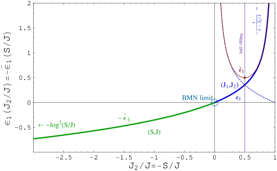
Figure 1: The leading order correction to the energy $\epsilon_{1}$ for the folded string solution. The region $J_{2}/J>0$ correspond to the $(J_{1},J_{2})$ case, whereas $J_{2}/J<0$ correspond to the $(S,J)$ case with $S/J=-J_{2}/J$ and energy $\tilde{\epsilon}_{1}=-\epsilon_{1}$. We also plot a mirror image under the symmetry $J_{1}\leftrightarrow J_{2}$ (dashed) and the energy of the circular string $\hat{\epsilon}_{1}$ (dotted).

For the $(J_{1},J_{2})$ solution the function $\epsilon_{1}(J_{2}/J)$ is defined in the region $0\leq J_{2}/J<1$ whereas for the $(S,J)$ solution $\tilde{\epsilon}_{1}(S/J)$ is naturally defined for $0\leq S/J<\infty$. When analytically continued, these functions are related by $\epsilon_{1}(j)=-\tilde{\epsilon}_{1}(-j)$. In Figure 1, we therefore plot the function $\epsilon_{1}(j)$ in the region $j\in(-\infty,1)$.

Depending on the region of the parameter space one finds different functional form of dependence of the energy on the two spins. For example, in the case of the $(S,J)$ solution there are two different asymptotics that were considered in [11]: The string can become very long and approach the boundary of $AdS_{5}$, i.e. $\rho_{0}\to\infty$; the energy of this configuration is

$$E=S+J+\frac{\lambda}{2\pi^{2}J}\,\ln^{2}\frac{S}{J}+\ldots\,,\qquad\ \ \ \ \ S\gg J\,.$$ (E.1)

In gauge theory this corresponds to the case where the two contours $\mathcal{C}^{\pm}$ meet, i.e. $a\to 0,b\to\infty$. A short string reproduces the energy of BMN operators correctly (all mode numbers are $n=\pm 1$)

$$E=J+S+\frac{\lambda\,S}{2J^{2}}+\ldots\ ,\qquad\ \ \ \ S\ll J\,.$$ (E.2)

One may also consider a “near BMN” limit $S/J\ll 1$ of the two-spin solution keeping full dependence on $\lambda$. Then we get

$$E=J+S\sqrt{1+\frac{\lambda}{J^{2}}}-\frac{\lambda\,S^{2}}{4J^{3}}\cdot\frac{2+\lambda/J^{2}}{1+\lambda/J^{2}}+\ldots\ ,\ \ \ \ \ \ \ S\ll J\ ,$$ (E.3)

This gives the near BMN limit for a total of $S$ excitations of modes $n=\pm 1$. Note, however, that we must consider a large number of excitations $S=\mathcal{O}(J)$, i.e. $S=\beta J$ with $\beta$ small but $\mathcal{O}(J^{0})$. Therefore, we may not assume that $S=\beta J$ takes a particular, finite value like, for example, two (in an attempt to compare to $1/J$ terms in [32]). Instead, one must consider an arbitrary number of excitations $S$ and consider only the coefficient $c$ in the near BMN correction $(cS+c^{\prime})/J=c\beta+\mathcal{O}(1/J)$. The point is that $c^{\prime}$ is an $\mathcal{O}(1/J)$ correction which we presently ignore.

At $S/J=0$ we make the “Wick-rotation” to the $(J_{1},J_{2})$ solution. The energy of a short string rotating on $S^{5}$ is given by

$$E=J+\frac{\lambda\,J_{2}}{2J^{2}}+\ldots\,,\qquad\ \ J_{2}\ll J\,,$$ (E.4)

where we can explicitly see the connection to the $(S,J)$ case. Similarly, the near BMN limit reads (we set $J_{1}=J$ to compare to BMN terminology, $J_{2}$ represents the number of excitations)

$$E=J_{1}+J_{2}\sqrt{1+\frac{\lambda}{J_{1}^{2}}}-\frac{\lambda\,J_{2}^{2}}{4J_{1}^{3}}\cdot\frac{2+3\lambda/J_{1}^{2}}{1+\lambda/J_{1}^{2}}+\ldots\ ,\ \ \ \ \ \ J_{2}\ll J\ .$$ (E.5)

As the charge $J_{2}$ increases, the string grows until for $J_{1}=J_{2}$ we get

$$E=J+c\frac{\lambda}{J}+\ldots\ ,\ \ \ c\equiv\epsilon_{1}(1/2)=0.356016\ldots\ ,\ \ \ \ \ J_{2}=J_{1}=J/2\ .$$ (E.6)

In string theory nothing special happens, the string extends over approximately $120^{\circ}$ and can grow further. In contrast, in gauge theory we made the assumption $J_{2}\leq J_{1}$ to solve the Bethe ansatz. Therefore, we do not get solutions beyond this point. Nevertheless, in terms of charges, we can freely interchange $J_{1}$ and $J_{2}$. The string solutions for $J_{2}>J/2$ should correspond to some gauge theory states with $J_{2}<J/2$

$$\delta^{\prime}_{1}(J_{2}/J)=\epsilon_{1}(1-J_{2}/J)\ ,\ \ \ \qquad\mbox{for }\ 0\leq J_{2}\leq J/2\ .$$ (E.7)

We see that the string energy $\epsilon_{1}(J_{1},J_{2})$ is not symmetric with respect to $J_{1}\leftrightarrow J_{2}$. As a consequence, the anomalous dimensions $\delta^{\prime}_{1}(J_{1},J_{2})$ do not belong to operators with the minimal energy, $\delta_{1}(J_{1},J_{2})$, but to some other set of operators with larger dimensions. That suggests that one and the same string solution describes two different operators in different regions of parameter space. There are some indications that these new gauge theory operators are the odd, unpaired ground state solutions found in [24]. This is an interesting possibility, as it would explain why for half-filling, $J_{2}=J/2$, the odd, unpaired ground state has energy (E.6) as suggested by numerical evidence [24]. Further numerical evidence shows that the anomalous dimension $\delta^{\prime}_{1}$ of this state near $J_{2}=0$ scales as $1/J_{2}$ instead of $1/J$. Indeed, this is what happens on the string theory side. The largest extension of the $S^{5}$ solution takes place near $J_{2}=J$. Then the string extends over half a great circle and the energy is

$$E=J+\frac{2\,\lambda}{\pi^{2}\,J(1-J_{2}/J)}+\ldots=J+\frac{2\,\lambda}{\pi^{2}\,J_{1}}+\ldots\ ,\ \ \ \ \ \ J_{2}\approx J\ .$$ (E.8)

At $J_{2}=J$ the folded string becomes, in fact, equivalent to a different configuration: One half of the string can be unfolded to give the circular string discussed in Appendix D. It is interesting to see that also the energy of the circular solution $\hat{\epsilon}_{1}$ asymptotes to the same value

$$E=J+\frac{2\,\lambda}{\pi^{2}\,J_{1}}+\ldots\ ,\ \ \ \ \ \ J_{2}\approx J\ .$$ (E.9)

The energy $\hat{\epsilon}_{1}$ of the circular solution decreases as we decrease $J_{2}$ up to half-filling $J_{2}=J_{1}=J$. Unlike in the case of the folded string, the energy has a minimum

$$E=J+\frac{\lambda}{2J}+\ldots\ ,\ \ \ \ \ \ J_{2}=J_{1}=J/2\ .$$ (E.10)

Furthermore, the solution $\hat{\epsilon}_{1}$ is symmetric under $J_{1}\leftrightarrow J_{2}$ and we can stop.

References

- [1] J. M. Maldacena, “The large N limit of superconformal field theories and supergravity”, Adv. Theor. Math. Phys. 2 (1998) 231, hep-th/9711200.
- [2] S. S. Gubser, I. R. Klebanov and A. M. Polyakov, “Gauge theory correlators from non-critical string theory”, Phys. Lett. B428 (1998) 105, hep-th/9802109.
- [3] E. Witten, “Anti-de Sitter space and holography”, Adv. Theor. Math. Phys. 2 (1998) 253, hep-th/9802150.
- [4] G. Arutyunov, S. Frolov and A. C. Petkou, “Operator product expansion of the lowest weight CPOs in 4 SYM4 at strong coupling”, Nucl. Phys. B586 (2000) 547, hep-th/0005182.
- [5] B. Eden, A. C. Petkou, C. Schubert and E. Sokatchev, “Partial non-renormalisation of the stress-tensor four-point function in 4 SYM4 and AdS/CFT”, Nucl. Phys. B607 (2001) 191, hep-th/0009106.
- [6] G. Arutyunov, F. A. Dolan, H. Osborn and E. Sokatchev, “Correlation functions and massive Kaluza-Klein modes in the AdS/CFT correspondence”, Nucl. Phys. B665 (2003) 273, hep-th/0212116.
- [7] D. Berenstein, J. M. Maldacena and H. Nastase, “Strings in flat space and pp waves from 4 Super Yang Mills”, JHEP 0204 (2002) 013, hep-th/0202021.
- [8] M. Blau, J. Figueroa-O’Farrill, C. Hull and G. Papadopoulos, “A new maximally supersymmetric background of IIB superstring theory”, JHEP 0201 (2002) 047, hep-th/0110242.
- [9] R. R. Metsaev, “Type IIB Green-Schwarz superstring in plane wave Ramond-Ramond background”, Nucl. Phys. B625 (2002) 70, hep-th/0112044.
- [10] S. S. Gubser, I. R. Klebanov and A. M. Polyakov, “A semi-classical limit of the gauge/string correspondence”, Nucl. Phys. B636 (2002) 99, hep-th/0204051.
- [11] S. Frolov and A. A. Tseytlin, “Semiclassical quantization of rotating superstring in ”, JHEP 0206 (2002) 007, hep-th/0204226.
- [12] A. A. Tseytlin, “Semiclassical quantization of superstrings: and beyond”, Int. J. Mod. Phys. A18 (2003) 981, hep-th/0209116.
- [13] J. G. Russo, “Anomalous dimensions in gauge theories from rotating strings in ”, JHEP 0206 (2002) 038, hep-th/0205244.
- [14] J. A. Minahan, “Circular semiclassical string solutions on ”, Nucl. Phys. B648 (2003) 203, hep-th/0209047.
- [15] G. Mandal, N. V. Suryanarayana and S. R. Wadia, “Aspects of semiclassical strings in ”, Phys. Lett. B543 (2002) 81, hep-th/0206103.
- [16] S. Frolov and A. A. Tseytlin, “Multi-spin string solutions in ”, Nucl. Phys. B668 (2003) 77, hep-th/0304255.
- [17] S. Frolov and A. A. Tseytlin, “Quantizing three-spin string solution in ”, JHEP 0307 (2003) 016, hep-th/0306130.
- [18] S. Frolov and A. A. Tseytlin, “Rotating string solutions: AdS/CFT duality in non-supersymmetric sectors”, Phys. Lett. B570 (2003) 96, hep-th/0306143.
- [19] G. Arutyunov, S. Frolov, J. Russo and A. A. Tseytlin, “Spinning strings in and integrable systems”, hep-th/0307191.
- [20] H. J. de Vega and I. L. Egusquiza, “Planetoid String Solutions in 3 + 1 Axisymmetric Spacetimes”, Phys. Rev. D54 (1996) 7513, hep-th/9607056.
- [21] A. Santambrogio and D. Zanon, “Exact anomalous dimensions of 4 Yang-Mills operators with large R charge”, Phys. Lett. B545 (2002) 425, hep-th/0206079.
- [22] J. A. Minahan and K. Zarembo, “The Bethe-ansatz for 4 super Yang-Mills”, JHEP 0303 (2003) 013, hep-th/0212208.
- [23] N. Beisert and M. Staudacher, “The 4 SYM Integrable Super Spin Chain”, Nucl. Phys. B670 (2003) 439, hep-th/0307042.
- [24] N. Beisert, J. A. Minahan, M. Staudacher and K. Zarembo, “Stringing Spins and Spinning Strings”, JHEP 0309 (2003) 010, hep-th/0306139.
- [25] N. Beisert, C. Kristjansen and M. Staudacher, “The dilatation operator of 4 conformal super Yang-Mills theory”, Nucl. Phys. B664 (2003) 131, hep-th/0303060.
- [26] N. Beisert, “The Complete One-Loop Dilatation Operator of 4 Super Yang-Mills Theory”, hep-th/0307015.
- [27] I. Bena, J. Polchinski and R. Roiban, “Hidden symmetries of the superstring”, hep-th/0305116.
- [28] R. R. Metsaev and A. A. Tseytlin, “Type IIB superstring action in background”, Nucl. Phys. B533 (1998) 109, hep-th/9805028.
- [29] L. Dolan, C. R. Nappi and E. Witten, “A Relation Between Approaches to Integrability in Superconformal Yang-Mills Theory”, hep-th/0308089.
- [30] A. V. Belitsky, A. S. Gorsky and G. P. Korchemsky, “Gauge/string duality for QCD conformal operators”, Nucl. Phys. B667 (2003) 3, hep-th/0304028.
- [31] N. Beisert, “Higher loops, integrability and the near BMN limit”, hep-th/0308074.
- [32] C. G. Callan, Jr., H. K. Lee, T. McLoughlin, J. H. Schwarz, I. Swanson and X. Wu, “Quantizing string theory in : Beyond the pp-wave”, hep-th/0307032.
- [33] I. K. Kostov and M. Staudacher, “Multicritical phases of the O(n) model on a random lattice”, Nucl. Phys. B384 (1992) 459, hep-th/9203030.
- [34] N. Muskhelishvili, “Singular integral equations”, Noordhoff NV (1953), Groningen, Netherlands.