First-order phase transitions in confined systems

Abstract

In a field-theoretical context, we consider the Euclidean $(\phi^{4}+\phi^{6})_{D}$ model compactified in one of the spatial dimensions. We are able to determine the dependence of the transition temperature ($T_{c}$) for a system described by this model, confined between two parallel planes, as a function of the distance ($L$) separating them. We show that $T_{c}$ is a concave function of $L^{-1}$. We determine a minimal separation below which the transition is suppressed.

PACS number(s): 03.70.+k, 11.10.-z

In the last few decades, a large amount of work has been done on field theoretical models applied to the study of critical phenomena. In particular, second-order phase transitions have been extensively studied in view of the investigation of several material systems. An account on the state of the subject and related topics can be found, for instance, in Refs. affleck -isaque . Questions concerning the existence of phase transitions may also be raised if one considers the behaviour of field theories as a function of spatial boundaries. The existence of phase transitions would be in this case associated to some spatial parameters describing the breaking of translational invariance, for instance, the distance $L$ between planes confining the system. Studies of this type have been recently performed malbouisson2 ; malbouisson3 , concerning with the spontaneous symmetry breaking in the $\lambda\phi^{4}$ theory. In particular, if one considers the Ginzburg–Landau model confined between two parallel planes, which is assumed to describe a film of some material, the question of how the critical temperature depends on the thickness $L$ of the film can be raised.

Studies on confined field theory have been done in the literature for a long time. In particular, an analysis of the renormalization group in finite size geometries can be found in zinn ; cardy . These studies have been performed to take into account boundary effects on scaling laws. In another related topic of investigation, there are systems that present domain walls as defects, created for instance in the process of crystal growth by some prepared circumstances. At the level of effective field theories, in many cases, this can be modeled by considering a Dirac fermionic field whose mass changes sign as it crosses the defect, meaning that the domain wall plays the role of a critical boundary separating two different states of the system fosco1 ; fosco2 .

Under the assumption that information about general features of the behaviour of systems undergoing phase transitions in absence of external influences (like magnetic fields) can be obtained in the approximation which neglects gauge field contributions in the Ginzburg–Landau model, investigations have been done with an approach different from the renormalization group analysis. It has been considered the system confined between two parallel planes and using the formalism developed in Refs. malbouisson2 ; malbouisson3 it has been investigated how the critical temperature is affected by the presence of boundaries. In particular a study has been done on how the critical temperature ($T_{c}$) of a superconducting film depends on its thickness $L$ luciano ; luciano1 . In this paper we perform a further step, by considering in the same context an extended model, which besides the quartic field self-interaction, a sextic one is also present. It is well known that those interactions, taken together, lead to renormalizable quantum field theories in three dimensions and that they are supposed to describe first-order phase transitions.

¿From our point of view, as in previous publications, the system to be studied is a slab of a material of thickness $L$, the behaviour of which in the critical region is to be derived from a quantum field theory calculation of the dependence of the renormalized mass parameter on $L$. We start from the effective potential for the theory, which is related to the renormalized mass through a renormalization condition. This condition, however, reduces considerably the number of relevant Feynman diagrams contributing to the mass renormalization, if one wishes to be restricted to first-order terms in both coupling constants of the model. In fact, just two diagrams need to be considered in this approximation: a tadpole graph with the $\phi^{4}$ coupling (1 loop) and a “shoestring” graph with the $\phi^{6}$ coupling (2 loops)(see Fig.1). No diagram with both couplings occur. The $L$-dependence appears from the treatment of the loop integrals, as the material is confined between two plane sheets a distance $L$ apart from one another. We therefore take the space dimension orthogonal to the planes as finite, the other two being otherwise infinite. This dimension of finite extent is treated in the momentum space using the formalism of Ref. malbouisson3 .

We start by stating the Ginzburg-Landau Hamiltonian density in a Euclidean $D$-dimensional space, now including both $\phi^{4}$ and $\phi^{6}$ interactions, in the absence of external fields, given by (in natural units, $\hbar=c=k_{B}=1$),

$$\mathcal{H}=\left|\nabla\varphi\right|^{2}+m_{0}^{2}\left|\varphi\right|^{2}+\frac{\lambda}{2}\left|\varphi\right|^{4}+\frac{\eta}{6}\left|\varphi\right|^{6},$$ (1)

where $\lambda$ and $\eta$ are the (renormalized) quartic and sextic self-coupling constants, with the bare mass given by $m_{0}^{2}=\alpha(T-T_{0})$, $T_{0}$ being the bulk transition temperature of the material and $\alpha>0$. We consider the system confined between two parallel planes, normal to the $x$-axis, a distance $L$ apart from one another and use Cartesian coordinates $\mathbf{r}=(x,\mathbf{z})$, where $\mathbf{z}$ is a ($D-1$)-dimensional vector, with corresponding momenta $\mathbf{k}=(k_{x},\mathbf{q}),\mathbf{q}$ being a ($D-1$)-dimensional vector in momenta space. The generating functional of Schwinger functions is written in the form

$$\mathcal{Z}=\int\mathcal{D\varphi}^{*}\mathcal{D\varphi}\exp\left(-\int_{0}^{L}dx\int d^{D-1}z\,\mathcal{H}\left(\left|\varphi\right|,\left|\nabla\varphi\right|\right)\right),$$ (2)

with the field $\varphi(x,\mathbf{z})$ satisfying the condition of confinement along the $x$-axis, $\varphi(x\leq 0,\mathbf{z})=\varphi(x\geq L,\mathbf{z})=$const. Then the field should have a mixed series-integral Fourier representation of the form

$$\varphi(x,\mathbf{z})=\sum_{n=-\infty}^{\infty}c_{n}\int d^{D-1}q\,b(\mathbf{q})e^{-i\omega_{n}x-i\mathbf{q}\cdot\mathbf{z}}\tilde{\varphi}(\omega_{n},\mathbf{q}),$$ (3)

where $\omega_{n}=2\pi n/L$ and the coefficients $c_{n}$ and $b(\mathbf{q})$ correspond respectively to the Fourier series representation over $x$ and to the Fourier integral representation over the ($D-1$)-dimensional $\mathbf{z}$-space. The above conditions of confinement of the $x$-dependence of the field to a segment of length $L$ allow us to proceed, with respect to the $x$-coordinate, in a manner analogous as is done in the imaginary-time Matsubara formalism in field theory and, accordingly, the Feynman rules should be modified following the prescription

$$\int\frac{dk_{x}}{2\pi}\rightarrow\frac{1}{L}\sum_{n=-\infty}^{\infty},\qquad k_{x}\rightarrow\frac{2n\pi}{L}\equiv\omega_{n}.$$ (4)

We emphasize, however, that we are considering an Euclidean field theory in $D$ purely spatial dimensions, so we are not working in the framework of finite-temperature field theory. Here, the temperature is introduced in the mass term of the Hamiltonian by means of the usual Ginzburg–Landau prescription.

To continue, we use some one-loop results described in malbouisson2 ; malbouisson3 ; ananos , adapted to our present situation. These results have been obtained by the concurrent use of dimensional and zeta-function analytic regularizations, to evaluate formally the integral over the continuous momenta and the summation over the frequencies $\omega_{n}$. We get sums of polar ($L$-independent) terms plus $L$-dependent analytic corrections. Renormalized quantities are obtained by subtraction of the divergent (polar) terms appearing in the quantities obtained by application of the modified Feynman rules and dimensional regularization formulas. These polar terms are proportional to $\Gamma$-functions having the dimension $D$ in the argument and correspond to the introduction of counterterms in the original Hamiltonian density. In order to have a coherent procedure in any dimension, those subtractions should be performed even for those values of the dimension $D$ for which no poles are present. In these cases a finite renormalization is performed.

In principle, the effective potential for systems with spontaneous symmetry breaking is obtained, following the Coleman–Weinberg analysis coleman , as an expansion in the number of loops in Feynman diagrams. Accordingly, to the free propagator and to the no-loop (tree) diagrams for both couplings, radiative corrections are added, with increasing number of loops. Thus, at the 1-loop approximation, we get the infinite series of 1-loop diagrams with all numbers of insertions of the $\phi^{4}$ vertex (two external legs in each vertex), plus the infinite series of 1-loop diagrams with all numbers of insertions of the $\phi^{6}$ vertex (four external legs in each vertex), plus the infinite series of 1-loop diagrams with all kinds of mixed numbers of insertions of $\phi^{4}$ and $\phi^{6}$ vertices. Analogously, we should include all those types of insertions in diagrams with 2 loops, etc. However, instead of undertaking such a daunting computation, even if we restrict ourselves to the lowest terms in the loop expansion, we remember that the gap equation we are seeking is given by the renormalization condition in which the renormalized squared mass is defined as the second derivative of the effective potential $U(\varphi_{0})$ with respect to the classical field $\varphi_{0}$, taken at zero field,

$$\left.\frac{\partial^{2}U(\varphi_{0})}{\partial\varphi_{0}{}^{2}}\right|_{\varphi_{0}=0}=m^{2}.$$ (5)

For our purposes, we do not need to consider the renormalization conditions for the interaction coupling constants, i.e., they may be considered as already renormalized when they are written in the Hamiltonian above. At the 1-loop approximation, the contribution of loops with only $\phi^{4}$ vertices to the effective potential is obtained directly from malbouisson3 , as an adaptation of the Coleman–Weinberg expression after compactification in one dimension,

$$U_{1}(\phi,L) = \mu^{D}\sqrt{a}\sum_{s=1}^{\infty}\frac{(-1)^{s+1}}{2s}g_{1}^{s}\phi_{0}^{2s}$$ (6)

$$\times\sum_{n=-\infty}^{\infty}\int\frac{d^{D-1}k}{\left(\mathbf{k}^{2}+an^{2}+c^{2}\right)^{s}}.$$

In the above formula, in order to deal with dimensionless quantities in the regularization procedure, we have introduced parameters $c^{2}=m^{2}/4\pi^{2}\mu^{2}$, $a=(L\mu)^{-2}$, $g_{1}=\lambda/8\pi^{2}$ and $\phi_{0}=\varphi_{0}/\mu$, where $\varphi_{0}$ is the normalized vacuum expectation value of the field (the classical field) and $\mu$ is a mass scale. The parameter $s$ counts the number of vertices on the loop.

It is easily seen that only the $s=1$ term contributes to the renormalization condition (5). It corresponds to the tadpole diagram. It is then also clear that all $\phi^{6}$-vertex and mixed $\phi^{4}$- and $\phi^{6}$-vertex insertions on the 1-loop diagrams do not contribute when one computes the second derivative of similar expressions with respect to the field at zero field: only diagrams with two external legs should survive. This is impossible for a $\phi^{6}$-vertex insertion at the 1-loop approximation, therefore the first contribution from the $\phi^{6}$ coupling must come from a higher-order term in the loop expansion. Two-loop diagrams with two external legs and only $\phi^{4}$ vertices are of second order in its coupling constant, and we neglect them, as well as all possible diagrams with vertices of mixed type. However, the 2-loop shoestring diagram, with only one $\phi^{6}$ vertex and two external legs is a first-order (in $\eta$) contribution to the effective potential, according to our renormalization criterion.

Figure 1: Diagrams contributing to the renormalized mass at lowest order in the coupling constants.

Therefore the renormalized mass is defined at first-order in both coupling constants, by the contributions of radiative corrections from only two diagrams: the tadpole and the shoestring diagrams. The tadpole contribution reads (putting $s=1$ in eq. (6)),

$$U_{1}(\phi_{0},L)=\mu^{D}\sqrt{a}\frac{1}{2}g_{1}\phi_{0}^{2}\sum_{n=-\infty}^{\infty}\int\frac{d^{D-1}k}{\mathbf{k}^{2}+an^{2}+c^{2}}.$$ (7)

The integral on the $D-1$ non-compactified momentum variables is performed using the dimensional regularization formula

$$\int\frac{d^{d}k}{k^{2}+M}=\frac{\Gamma\left(1-\frac{d}{2}\right)\pi^{d/2}}{M^{1-d/2}};$$ (8)

for $d=D-1$, we obtain

$$U_{1}(\phi_{0},L) = \mu^{D}\sqrt{a}\frac{\pi^{(D-1)/2}}{2}g_{1}\phi_{0}^{2}\Gamma\left(\frac{3-D}{2}\right)$$ (9)

$$\times\sum_{n=-\infty}^{\infty}\frac{1}{(an^{2}+c^{2})^{(3-D)/2}}.$$

The sum in the above expression may be recognized as one of the Epstein–Hurwitz zeta-functions, $Z_{1}^{c^{2}}(\frac{3-D}{2};a)$, which may be analytically continued to elizalde

$$Z_{1}^{c^{2}}(\nu;a) = \frac{2^{\frac{2\nu+1}{2}}\pi^{\frac{4\nu-1}{2}}}{\sqrt{a}\Gamma(\nu)}\left[2^{\nu-3/2}\left(\frac{m}{\mu}\right)^{1-2\nu}\Gamma\left(\nu-\frac{1}{2}\right)\right.$$

$$\left.+2\sum_{n=1}^{\infty}\left(\frac{m}{\mu^{2}Ln}\right)^{1/2-\nu}K_{\nu-1/2}(mnL)\right],$$

where the $K_{\nu}$ are Bessel functions of the third kind. The tadpole part of the effective potential is then

$$U_{1}(\phi_{0},L) = \frac{\mu^{D}g_{1}\phi_{0}^{2}}{\left(2\pi\right)^{D/2-2}}\left[2^{-\frac{D+1}{2}}\left(\frac{m}{\mu}\right)^{D-2}\Gamma\left(1-\frac{D}{2}\right)\right.$$

$$\left.+\sum_{n=1}^{\infty}\left(\frac{m}{\mu^{2}Ln}\right)^{D/2-1}K_{D/2-1}(mnL)\right].$$

Notice that since we are using dimensional regularization techniques, there is implicit in the above formulas a factor $\mu^{4-D}$ in the definition of the coupling constant $\lambda$. In what follows we make explicit this factor, the symbol $\lambda$ standing for the dimensionless coupling parameter (which coincides with the physical coupling constant in $D=4$).

We now turn to the 2-loop shoestring diagram contribution to the effective potential, using again the Feynman rule prescription for the compactified dimension. It reads

$$U_{2}(\phi,L)=\mu^{2D-2}a\frac{1}{2}g_{2}\phi_{0}^{2}\left[\frac{\Gamma\left(\frac{3-D}{2}\right)}{\left(4\pi\right)^{(D-1)/2}}Z_{1}^{c^{2}}\left(\frac{3-D}{2};a\right)\right]^{2},$$ (12)

or, after subtraction of the polar term coming from the first term of Eq.(LABEL:epstein),

$$U_{2}^{\rm(Ren)}(\phi,L)=\frac{\eta\mu^{6-2D}\varphi_{0}^{2}}{8(2\pi)^{3D-2}}\left[\sum_{n=1}^{\infty}\left(\frac{m}{nL}\right)^{D/2-1}K_{\frac{D-2}{2}}(mnL)\right]^{2}.$$ (13)

The renormalized mass with both contributions then satisfies an $L$-dependent generalized Dyson–Schwinger equation,

$$m^{2}(L) = m_{0}^{2}-\frac{\beta}{\left(2\pi\right)^{D/2}}\sum_{n=1}^{\infty}\left(\frac{m}{nL}\right)^{D/2-1}K_{\frac{D-2}{2}}(mnL)$$

$$+\frac{\rho}{8(2\pi)^{3D-2}}\left[\sum_{n=1}^{\infty}\left(\frac{m}{nL}\right)^{D/2-1}K_{\frac{D-2}{2}}(mnL)\right]^{2},$$

where we have introduced the dimensionful coupling constants $\beta=-\lambda\mu^{4-D}$ and $\rho=\eta\mu^{6-2D}$.

A first-order transition occurs when all the three minima of the potential

$$V(\varphi_{0})=m(L)^{2}\varphi_{0}^{2}-\frac{\beta}{2}\varphi_{0}^{4}+\frac{\rho}{6}\varphi_{0}^{6},$$ (15)

where $m(L)$ is the renormalized mass defined above, are simultaneously on the line $V(\varphi_{0})=0$. This gives the condition

$$m^{2}=\frac{3\beta^{2}}{4\rho}.$$ (16)

Notice that the value $m=0$ is excluded in the above condition, for it corresponds to a second-order transition. For $D=3$, which is the physically interesting situation of the system confined between two parallel planes embedded in a 3-dimensional Euclidean space, the Bessel functions entering in the above equations have an explicit form, $K_{1/2}(z)=\sqrt{\pi}e^{-z}/\sqrt{2z}$, which replaced in Eq.(LABEL:massren1) and performing the resulting sum gives

$$m^{2}(L) = \alpha(T-T_{0})+\frac{\beta}{\left(2\pi\right)^{3/2}}\sqrt{\frac{\pi}{2}}\frac{1}{L}\log(1-e^{-mL})$$

$$+\frac{\rho\pi}{8(2\pi)^{7}L^{2}}\left[\log(1-e^{-mL})\right]^{2}.$$

Taking $m=1$ in Eq.(16), we get the critical temperature,

$$T_{c}(L) = \frac{T_{0}+1}{\alpha}-\frac{\beta}{\left(2\pi\right)^{3/2}}\sqrt{\frac{\pi}{2}}\frac{1}{L}\log(1-e^{-mL})$$ (18)

$$-\frac{3\beta^{2}\pi}{32(2\pi)^{7}L^{2}}\left[\log(1-e^{-mL})\right]^{2}.$$

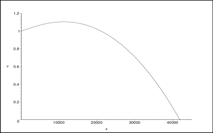
Figure 2: Relative critical temperature $v=T_{c}/T_{0}$ as a function of the inverse thickness $x=1/L$, in natural units ($m^{-1}$) with $T_{0}=4000,\;\alpha=1,\;\beta=0.1\;\rho=0.3/4$.

A plot of the relative critical temperature $T_{c}/T_{0}$ against the inverse thickness of the system from the above equation, is given in Fig.2 for, in natural units, $\alpha=1{\rm m}^{-1}$,$\beta=0.1{\rm m}^{-1}$ and $T_{0}=4000{\rm m}^{-1}$ ($\approx 10^{\rm o}$K). We see from the figure that the critical temperature slightly grows above the bulk transition temperature as the thickness of the system diminishes, reaching a maximum and afterwards starting to decrease until a zero value, corresponding to a minimal allowed thickness for the system. This behaviour may be contrasted with the linear decreasing of $T_{c}$ from the maximum value $T_{0}$ with the inverse of the thickness of the system, that has been found for second-order transitions luciano ; urucubaca . We also remark that in $D=3$, for second-order transitions, one considers $m=0$ and that leads to the need of a pole-subtraction procedure for the mass isaque . In our case such a procedure is not necessary, as a first-order transition must occur for a non-zero value of the mass. This fact, together with the closed formula for the Bessel function for $D=3$, allows us to obtain the exact expression (18) for the critical temperature.

This work has received partial financial support from CNPq and Pronex.

References

- (1) I. Affleck and E. Brézin, Nucl. Phys. 257 (1985) 451.
- (2) I.D. Lawrie, Phys. Rev. B 50 (1994) 9456.
- (3) I.D. Lawrie, Phys. Rev. Lett. 79 (1997) 131.
- (4) E. Brézin, D.R. Nelson and A. Thiaville, Phys. Rev. B 31 (1985) 7124.
- (5) L. Razihovsky, Phys. Rev. Lett. 74 (1995) 4722.
- (6) C. de Calan, A.P.C. Malbouisson and F.S. Nogueira, Phys. Rev. B 64 (2001) 212502.
- (7) A.P.C. Malbouisson, F.S. Nogueira and N.F. Svaiter, EuroPhys. Lett. 41 (1998) 547.
- (8) L. Halperin, T. C. Lubensky, S-K. Ma, Phys. Rev. Lett. 32, 292(1974).
- (9) L.M. Abreu, A.P.C. Malbouisson, I. Roditi, cond-mat/0305368, to appear in Physica A (2003).
- (10) C.D. Fosco and A. Lopez, Nucl. Phys. B 538 (1999) 685.
- (11) L. Da Rold, C.D. Fosco and A.P.C. Malbouisson, Nucl. Phys. B 624 (2002) 485.
- (12) J. Zinn-Justin, Quantum Field Theory and Critical Phenomena (Clarendon Press, Oxford, 1996), chapter 36.
- (13) J.L. Cardy (ed.), Finite Size Scaling (North Holland, Amsterdam, 1988).
- (14) A.P.C. Malbouisson and J.M.C. Malbouisson, J. Phys. A: Math. Gen. 35 (2002) 2263.
- (15) A.P.C. Malbouisson, J.M.C. Malbouisson and A.E. Santana, Nucl. Phys. B 631 (2002) 83.
- (16) L.M. Abreu, A.P.C. Malbouisson, J.M.C. Malbouisson, A.E. Santana, Phys. Rev. B 67, 212502 (2003).
- (17) A.P.C. Malbouisson, J.M.C. Malbouisson and A.E. Santana, cond-mat/0205176.
- (18) A.P.C. Malbouisson, Phys. Rev. B, 66, 092502 (2002).
- (19) G.N.J. Añaños, A.P.C. Malbouisson and N.F. Svaiter, Nucl. Phys. B 547 (1999) 221.
- (20) S. Coleman and E. Weinberg, Phys. Rev. D 7 (1973) 1888.
- (21) A. Elizalde and E. Romeo, J. Math. Phys. 30 (1989) 1133.