On the energy-momentum tensor for a scalar field on manifolds with boundaries

Abstract

We argue that already at classical level the energy-momentum tensor for a scalar field on manifolds with boundaries in addition to the bulk part contains a contribution located on the boundary. Using the standard variational procedure for the action with the boundary term, the expression for the surface energy-momentum tensor is derived for arbitrary bulk and boundary geometries. Integral conservation laws are investigated. The corresponding conserved charges are constructed and their relation to the proper densities is discussed. Further we study the vacuum expectation value of the energy-momentum tensor in the corresponding quantum field theory. It is shown that the surface term in the energy-momentum tensor is essential to obtain the equality between the vacuum energy, evaluated as the sum of the zero-point energies for each normal mode of frequency, and the energy derived by the integration of the corresponding vacuum energy density. As an application, by using the zeta function technique, we evaluate the surface energy for a quantum scalar field confined inside a spherical shell.

PACS numbers: 03.50.Kk, 03.70.+k, 04.62.+v, 11.30.-j

1 Introduction

In many problems we need to consider the physical model on background of manifolds with boundaries on which the dynamical variables satisfy some prescribed boundary conditions. In presence of boundaries new degrees of freedom appear, which can essentially influence the dynamics of the model. The incomplete list of branches where the boundary effects play an important role includes: surface and finite-size effects in condensed matter theory and statistical physics, theory of phase transitions and critical phenomena [1, 2], canonical formulation of general relativity (see [3]), the definition of the gravitational action, Hamiltonian and energy-momentum [4]–[16], path-integral approach to quantum gravity and the problem of boundary conditions for the quantum state of the universe (see, for instance, [17] and references therein), bag models of hadrons in QCD, string and M-theories, various braneworld models, manifolds with horizons and the thermodynamics of black holes, AdS/CFT correspondence [18], holographic principle [19, 20]. In recent years, the study of the boundary effects in quantum theory has produced several important results. For example, an interesting idea is to consider the black hole event horizon as a physical boundary [21]. This induce an extra term in the action, having as consequence the existence of a central charge in the algebra of generators of gauge transformations. Using this central charge it is possible to determine the asymptotic behavior of the densities of states and in this way to get the entropy for a black hole [22]. In the context of string theory, the D-branes are natural boundaries for the open strings, having very interesting effects in the theory.

In quantum field theory the influence of boundaries on the vacuum state of a quantized field leads to interesting physical consequences. The imposition of boundary conditions leads to the modification of the zero–point fluctuations spectrum and results in the shifts in the vacuum expectation values of physical quantities, such as the energy density and vacuum stresses. In particular, vacuum forces arise acting on constraining boundaries. This is the familiar Casimir effect. The particular features of the resulting vacuum forces depend on the nature of the quantum field, the type of spacetime manifold and its dimensionality, on the boundary geometries and the specific boundary conditions imposed on the field. Since the original work by Casimir in 1948 [23] many theoretical and experimental works have been done on this problem, including various types of bulk and boundary geometries (see, e.g., [24]–[31] and references therein). The Casimir force has recently been measured with a largely improved precision [32] (for a review see [28, 33]) which allows for an accurate comparision between the experimental results and theoretical predictions. An essential point in the investigations of the Casimir effect is the relation between the mode sum energy, evaluated as the sum of the zero-point energies for each normal mode of frequency, and the volume integral of the renormalized energy density. For scalar fields with general curvature coupling in Ref. [34] it has been shown that in the discussion of this question for the Robin parallel plates geometry it is necessary to include in the energy a surface term concentrated on the boundary (see Refs. [35, 36] for similar issues in spherical and cylindrical boundary geometries and the discussion in Ref. [37]). However, in Refs. [34, 35, 36] the surface energy density is considered only for the case of the Minkowski bulk with static boundaries. In the present paper, by using the standard variational procedure, we derive an expression of the surface energy-momentum tensor for a scalar field with general curvature coupling parameter in the general case of bulk and boundary geometries. It is well-known that the imposition of boundary conditions leads to a vacuum expectation value of the energy-momentum tensor with non-integrable divergences as the boundary is approached [38, 39, 40]. The role of surface action to cancel these divergencies is emphasized in Ref. [40], where it has been shown that the finiteness of the total energy of a quantized field in a bounded region is a direct consequence of renormalization of bare surface actions. How boundary corrections are implemented by surface interaction and the structure of the corresponding counterterms in the renormalization procedure are discussed in Ref. [41] within the Schrödinger representation of quantum field theory. By suitably modifying the classical action with boundary corrections, in Ref. [42] it has been shown that for scalar fields confined in a cavity familiar functional methods can be applied and the functional measure is constructed by treating the boundary conditions as field equations coming from a variational procedure. Surface terms play an important role in the recently proposed procedure [11] (see also [12]–[15] and references therein) to regularize the divergencies of the gravitational action on noncompact space. By adding suitable boundary counterterms to the gravitational action, one can obtain a well-defined boundary energy-momentum tensor and a finite Euclidean action for the black hole spacetimes.

This paper is organized as follows. In Sec. 2 the notations are introduced for the geometrical quantities describing the manifold and the structure of the action is discussed. In Sec. 3 the variations of the bulk and surface actions are considered with respect to variations of the metric tensor and the expressions for the bulk and surface energy-momentum tensors are derived. The integral conservation laws described by these tensors are studied in Sec. 4. The expressions for the corresponding energy-momenta are derived and relations to the proper densities are discussed. The vacuum expectation values of the energy-momentum tensor for a scalar field on a static manifold with boundary are considered in Sec. 5. It is argued that the surface part of the energy density is essential to obtain the equality between the vacuum energy, evaluated as the sum of the zero-point energies for each normal mode, and the energy obtained by the integration of the corresponding vacuum energy density. As an application of general foemula, in Sec. 6 we consider the surface energy for a quantum scalar field confined inside a spherical shell. Section 7 concludes the main results of the paper. An integral representation of the partial zeta function needed for the calculation of the surface energy on a spherical shell is derived in Appendix A.

2 Notations and the action

Consider a $D+1$ - dimensional spacetime region $M$ with metric $g_{ik}$ and boundary $\partial M$. We assume that the spacetime $M$ is foliated into a family of spacelike hypersurfaces ${\Sigma}$ defined by $t={\mathrm{const}}$. The boundary of $M$ consists of the initial and final spacelike hypersurfaces $\Sigma_{1}$ and $\Sigma_{2}$, as well as a timelike smooth boundary $\partial M_{s}$ and, hence, $\partial M=\Sigma_{1}\cup\Sigma_{2}\cup\partial M_{s}$. The boundary of each ${\Sigma}$ we will denote $\partial{\Sigma}$: $\partial\Sigma=\Sigma\cap\partial M_{s}$. The corresponding spacetime region is depicted in Fig. 1 for a three dimensional $M$. The inward pointing unit normal vector field on $\partial M$ is denoted $n^{i}$. This vector is normalized in accordance with $n_{i}n^{i}=\epsilon$, where $\epsilon=1$ and $-1$ for spacelike and timelike boundary elements, respectively. We define $u^{i}$ as the future pointing unit normal vector to the spacelike hypersurfaces $\Sigma$. On the hypersurfaces $\Sigma_{1}$ and $\Sigma_{2}$ this vector is connected to the vector $n^{i}$ by relations: $u^{i}=n^{i}$ on $\Sigma_{1}$ and $u^{i}=-n^{i}$ on $\Sigma_{2}$. In the consideration below we will not assume that the timelike boundary $\partial M_{s}$ is orthogonal to the foliation of the spacetime. We define $\tilde{u}^{i}$ as the forward pointing timelike unit normal vector field to the surfaces $\partial\Sigma$ in the hypersurface $\partial M_{s}$. By construction one has $\tilde{u}^{i}n_{i}=0$. We further define $\tilde{n}^{i}$ as the vector field defined on $\partial M_{s}$ such that $\tilde{n}^{i}$ is the unit normal vector to $\partial\Sigma$ in hypersurface $\Sigma$ and, hence, by construction $u^{i}\tilde{n}_{i}=0$. It can be seen that the following relations take place between the introduced vectors (see, for instance, [8, 10, 16])

$$\tilde{n}^{i}=\lambda\left(n^{i}-\eta u^{i}\right),\quad\tilde{u}^{i}=\lambda\left(u^{i}+\eta n^{i}\right)\ ,$$ (2.1)

where $n^{i}$ is understood as the normal to $\partial M_{s}$, the variable $\eta=u^{i}n_{i}$ measures the non-orthogonality and $\lambda=1/\sqrt{1+\eta^{2}}$. For $\eta=0$ the foliation surfaces are orthogonal to the boundary $\partial M_{s}$. Note that the quantity $\lambda$ is connected to the proper radial velocity $v$ by the relation [16] $\lambda=\sqrt{1-v^{2}}$.

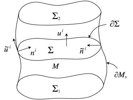
Figure 1: Manifold $M$ with boundary $\partial M=\Sigma_{1}\cup\Sigma_{2}\cup\partial M_{s}$ foliated by spacelike hypersurfaces ${\Sigma}$ with boundaries $\partial{\Sigma}$. $n^{i}$ and $u^{i}$ are unit normal vector fields to the hypersurfaces $\partial M_{s}$ and $\Sigma$ respectively. $\tilde{n}^{i}$ is the unit normal vector to the $(D-1)$-surface $\partial\Sigma$ in the hypersurface $\Sigma$, and $\tilde{u}^{i}$ is the unit normal vector to $\partial\Sigma$ in the hypersurface $\partial M_{s}$.

In the present paper we deal with a real scalar field $\varphi(x)$ propagating on the manifold $M$. The action describing the dynamics of the field we will take in the form

$$S=S_{b}+S_{s},$$ (2.2)

where the first term on the right,

$$S_{b}=\frac{1}{2}\int_{M}d^{D+1}x\sqrt{|g|}\left(\nabla_{i}\varphi\nabla^{i}\varphi-m^{2}\varphi^{2}-\zeta R\varphi^{2}\right),$$ (2.3)

is the standard bulk action for the scalar field with curvature coupling parameter $\zeta$, $R$ is the Ricci scalar for the manifold $M$, $\nabla_{i}$ is the covariant derivative operator associated with the bulk metric $g_{ik}$ (we adopt the conventions of Ref. [43] for the metric signature and the curvature tensor). The second term on the right of Eq. (2.2),

$$S_{s}=-\epsilon\int_{\partial M}d^{D}x\sqrt{|h|}\left(\zeta\varphi^{2}K+m_{s}\varphi^{2}\right),$$ (2.4)

is the surface action with a parameter $m_{s}$. In Eq. (2.4), $h$ is the determinant of the induced metric $h_{ik}$ for the boundary $\partial M$,

$$h_{ik}=g_{ik}-\epsilon n_{i}n_{k},$$ (2.5)

which acts as a projection tensor onto $\partial M$, $K$ is the trace of the extrinsic curvature tensor $K_{ik}$ of the boundary $\partial M$:

$$K=g^{ik}K_{ik}=h^{ik}K_{ik},\quad K_{ik}=h^{l}_{i}h^{m}_{k}\nabla_{l}n_{m},\quad h^{l}_{i}=g^{lk}h_{ik}.$$ (2.6)

For the most important special cases of minimally and conformally coupled scalars in Eq. (2.3) we have $\zeta=0,(D-1)/4D$, respectively. Note that in Eq. (2.4) the term with the extrinsic curvature scalar corresponds to the Gibbons-Hawking surface term in general relativity, $-\epsilon\int_{\partial M}d^{D}x\sqrt{|h|}\,K$. This term is required so that the action yields the correct equations of motion subject only to the condition that the induced metric on the boundary is held fixed. Note that for non-smooth boundary hypersurfaces it is necessary to add to action (2.2) the corner terms (for these terms in the gravitational action of general relativity see [7, 9, 10, 16]) with integrations over $(D-1)$-hypersurfaces at which the unit normal $n^{i}$ changes direction discontinously. As we have assumed a smooth boundary $\partial M_{s}$, in our case these hypersurfaces are presented by the $(D-1)$-surfaces $\partial\Sigma_{1}=\Sigma_{1}\cap\partial M_{s}$ and $\partial\Sigma_{2}=\Sigma_{2}\cap\partial M_{s}$ and the corresponding corner term in the action has the form

$$S_{c}=-\zeta\int_{\partial\Sigma_{1}}^{\partial\Sigma_{2}}d^{D-1}x\sqrt{|\sigma|}\,\varphi^{2}\,{\mathrm{arcsinh}}(\eta),$$ (2.7)

where $\int_{\partial\Sigma_{1}}^{\partial\Sigma_{2}}=\int_{\partial\Sigma_{2}}-\int_{\partial\Sigma_{1}}$ and $\sigma$ is the determinant of the metric tensor

$$\sigma_{ik}=g_{ik}+n_{i}n_{k}-\tilde{u}_{i}\tilde{u}_{k}=g_{ik}+\tilde{n}_{i}\tilde{n}_{k}-u_{i}u_{k}$$ (2.8)

induced on $\partial\Sigma$. In this paper we are interested in the variation of the action with respect to the variations for which the metric and field are held fixed on the initial and final spacelike hypersurfaces $\Sigma_{1}$ and $\Sigma_{2}$, and consequently on $\partial\Sigma_{1}$ and $\partial\Sigma_{2}$. In this case the corner terms will not contribute to the variations under consideration and we will omit them in the following consideration (see, however, the discussion after formula (3.27) in Sec. 3 for the total divergence term in the variation of the action, located on the boundary). Note that the contribution of the corner terms will be important in the case of a non-smooth boundary $\partial M_{s}$ having wedge-shaped parts.

3 Variation of the action and the energy-momentum tensor

3.1 Variation of the bulk action and the volume energy-momentum tensor

In this subsection we consider the variation of the bulk action (2.3) induced by an infinitesimal variation $\delta g_{ik}$ in the metric tensor. As the careful analysis of the surface terms is crucial for our discussion we will present the calculations in detail (for the corresponding calculations in general relativity see, for instance, [16]). To find the expression for the energy-momentum tensor of the scalar field with action (2.2), we need the variation of this action induced by an infinitesimal variation $\delta g_{ik}$ in the metric tensor.

First of all we consider the variation of the term involving the Ricci scalar:

$$\delta_{g}\int_{M}d^{D+1}x\sqrt{|g|}\,\varphi^{2}R=\int_{M}d^{D+1}x\sqrt{|g|}\,\varphi^{2}\left(\delta g^{ik}G_{ik}+g^{ik}\delta R_{ik}\right),$$ (3.1)

where $R_{ik}$ and $G_{ik}=R_{ik}-g_{ik}R/2$ are Ricci and Einstein tensors, respectively. To evaluate the second term in the braces on the right we note that the contracted variation $g^{ik}\delta R_{ik}$ is a pure spacetime divergence,

$$g^{ik}\delta R_{ik}=-\nabla_{l}W^{l},\quad W^{l}=g^{ik}\delta\Gamma_{ik}^{l}-g^{il}\delta\Gamma_{ik}^{k},$$ (3.2)

with $\Gamma_{ik}^{l}$ being the Christoffel symbol. In order to find the variations of the Christoffel symbol in this formula, note that from the identity $\delta(\nabla_{i}g_{kl})=0$ it follows

$$g^{ik}\delta\Gamma_{ik}^{l}=-g^{il}\delta\Gamma_{ik}^{k}+g^{lk}g^{ip}\nabla_{p}\delta g_{ik}.$$ (3.3)

Combining this with the relations

$$\delta\Gamma_{ik}^{k}=\nabla_{i}(\delta\ln\sqrt{|g|})=-\frac{1}{2}g_{lm}\nabla_{i}(\delta g^{lm}),\quad g^{lk}g^{ip}\nabla_{p}\delta g_{ik}=-\nabla_{m}(\delta g^{lm}),$$ (3.4)

one finds

$$W^{l}=g^{il}g_{km}\nabla_{i}(\delta g^{km})-\nabla_{m}(\delta g^{lm}).$$ (3.5)

By taking into account formula (3.2) and using the Stoke’s theorem

$$\int_{M}d^{D+1}x\sqrt{|g|}\,\nabla_{i}V^{i}=-\epsilon\int_{\partial M}d^{D}x\sqrt{|h|}\,n_{i}V^{i},$$ (3.6)

for the term with the variation of the Ricci tensor one has

$$\int_{M}d^{D+1}x\sqrt{|g|}\,\varphi^{2}g^{ik}\delta R_{ik}=\int_{M}d^{D+1}x\sqrt{|g|}\,W^{l}\nabla_{l}\varphi^{2}+\epsilon\int_{\partial M}d^{D}x\sqrt{|h|}\,\varphi^{2}n_{l}W^{l}.$$ (3.7)

For the first term on the right, using formula (3.5), we find

$$\int_{M}d^{D+1}x\sqrt{|g|}\,W^{l}\nabla_{l}\varphi^{2} = \int_{M}d^{D+1}x\sqrt{|g|}\,\delta g^{ik}\left(\nabla_{i}\nabla_{k}\varphi^{2}-g^{lm}g_{ik}\nabla_{l}\nabla_{m}\varphi^{2}\right)$$ (3.8)

$$+\epsilon\int_{\partial M}d^{D}x\sqrt{|h|}\,\delta g^{ik}\left(n_{i}\nabla_{k}\varphi^{2}-g_{ik}n^{l}\nabla_{m}\varphi^{2}\right).$$

Substituting this into formula (3.7) and taking into account formula (3.5), for the term containing the variation of the Ricci scalar, Eq. (3.1), we obtain the formula

$$\delta_{g}\int_{M}d^{D+1}x\sqrt{|g|}\,\varphi^{2}R = \int_{M}d^{D+1}x\sqrt{|g|}\,\delta g^{ik}\left(\varphi^{2}G_{ik}-g_{ik}g^{lm}\nabla_{l}\nabla_{m}\varphi^{2}+\nabla_{i}\nabla_{k}\varphi^{2}\right)$$

$$+\epsilon\int_{\partial M}d^{D}x\sqrt{|h|}\left\{\delta g^{ik}\left(n_{i}\nabla_{k}\varphi^{2}-g_{ik}n^{l}\nabla_{l}\varphi^{2}\right)\right.$$

$$+\left.\varphi^{2}\left[g_{km}n^{i}\nabla_{i}(\delta g^{km})-n_{l}\nabla_{m}(\delta g^{lm})\right]\right\}.$$

This leads to the following variation of the bulk action

$$\delta_{g}S_{b} = \frac{1}{2}\int_{M}d^{D+1}x\sqrt{|g|}\,\delta g^{ik}T_{ik}^{\mathrm{(vol)}}+\frac{\epsilon}{2}\int_{\partial M}d^{D}x\sqrt{|h|}\left\{\delta g^{ik}\left(-\zeta n_{i}\nabla_{k}\varphi^{2}\right.\right.$$ (3.10)

$$+\left.\left.\zeta g_{ik}n^{l}\nabla_{l}\varphi^{2}\right)+\zeta\varphi^{2}\left[n_{l}\nabla_{m}(\delta g^{lm})-g_{km}n^{i}\nabla_{i}(\delta g^{km})\right]\right\},$$

where $T_{ik}^{(\mathrm{vol})}$ is the standard metric energy-momentum tensor for a scalar field with a curvature coupling parameter $\zeta$ (see, for instance, [43]):

$$T_{ik}^{\mathrm{(vol)}}=\nabla_{i}\varphi\nabla_{k}\varphi-\frac{1}{2}g_{ik}g^{lm}\nabla_{l}\varphi\nabla_{m}\varphi+\frac{m^{2}}{2}\varphi^{2}g_{ik}-\zeta\varphi^{2}G_{ik}+\zeta g_{ik}g^{lm}\nabla_{l}\nabla_{m}\varphi^{2}-\zeta\nabla_{i}\nabla_{k}\varphi^{2}.$$ (3.11)

Note that this expression can be also written in the form

$$T_{ik}^{\mathrm{(vol)}}=T_{ik}^{(1)}+\frac{1}{2}\varphi g_{ik}\left(g^{lm}\nabla_{l}\nabla_{m}\varphi+\zeta R\varphi+m^{2}\varphi\right),$$ (3.12)

where

$$T_{ik}^{(1)}=\nabla_{i}\varphi\nabla_{k}\varphi+\left[\left(\zeta-\frac{1}{4}\right)g_{ik}g^{lm}\nabla_{l}\nabla_{m}-\zeta R_{ik}-\zeta\nabla_{i}\nabla_{k}\right]\varphi^{2}.$$ (3.13)

This tensor does not explicitly depend on the corresponding mass. For the covariant divergences of tensors (3.11) and (3.13) it can be seen that

$$\nabla_{i}T_{k}^{{\mathrm{(vol)}}i} = \left(g^{lm}\nabla_{l}\nabla_{m}\varphi+\zeta R\varphi+m^{2}\varphi\right)\nabla_{k}\varphi,$$ (3.14)

$$\nabla_{i}T_{k}^{(1)i} = -\frac{\varphi^{2}}{2}\nabla_{k}\left[\frac{1}{\varphi}\left(g^{lm}\nabla_{l}\nabla_{m}\varphi+\zeta R\varphi+m^{2}\varphi\right)\right].$$ (3.15)

From formula (3.10) it follows that the surface term in the variation of the bulk action contains the derivatives of the variation for the metric. In next subsection we will see that these terms are cancelled by the terms coming from the variation of surface action (2.4).

3.2 Variation of the surface action and the surface energy-momentum tensor

Now we turn to the evaluation of the variation for surface action (2.4) induced by the variation of the metric tensor. This variation can be written in the form

$$\delta_{g}S_{s}=-\epsilon\int_{\partial M}d^{D}x\sqrt{|h|}\left[\zeta\varphi^{2}\delta_{g}K+\frac{1}{2}h^{ik}\delta g_{ik}\left(\zeta\varphi^{2}K+m_{s}\varphi^{2}\right)\right].$$ (3.16)

First of all we note that for the variation of the extrinsic curvature tensor trace one has

$$\delta_{g}K=\delta_{g}(g^{ik}\nabla_{i}n_{k})=\delta g^{ik}\nabla_{i}n_{k}+g^{ik}\nabla_{i}\delta n_{k}-n_{l}g^{ik}\delta\Gamma_{ik}^{l}.$$ (3.17)

By making use formulae

$$\delta n_{i}=\frac{1}{2}\epsilon n_{i}n^{k}n^{l}\delta g_{kl},\quad\nabla_{i}n_{k}=K_{ik}+\epsilon n_{i}n^{l}\nabla_{l}n_{k},$$ (3.18)

and formula (3.3) for the contracted variation of the Christoffel symbol, it can be seen that

$$\delta_{g}K=-K^{ik}\delta g_{ik}+\frac{\epsilon}{2}Kn^{i}n^{k}\delta g_{ik}+n^{i}h^{kl}\left(\frac{1}{2}\nabla_{i}\delta g_{kl}-\nabla_{k}\delta g_{il}\right).$$ (3.19)

Substituting this relation into formula (3.16), for the variation of the surface action one finds

$$\delta_{g}S_{s} = -\epsilon\zeta\int_{\partial M}d^{D}x\sqrt{|h|}\,\varphi^{2}\left[\delta g_{ik}\left(-K^{ik}+\frac{1}{2}Kh^{ik}+\frac{\epsilon}{2}Kn^{i}n^{k}+\frac{m_{s}}{2\zeta}h^{ik}\right)\right.$$ (3.20)

$$\left.+n^{i}h^{kl}\left(\frac{1}{2}\nabla_{i}\delta g_{kl}-\nabla_{k}\delta g_{il}\right)\right].$$

By taking into account that in Eq. (3.10) we can replace

$$n_{l}\nabla_{m}(\delta g^{lm})-g_{km}n^{i}\nabla_{i}(\delta g^{km})=g^{km}n^{l}\left[\nabla_{l}(\delta g_{km})-\nabla_{m}(\delta g_{lk})\right],$$ (3.21)

and using formulae (3.10) and (3.20), for the variation of the total action one finds

$$\delta_{g}S = \frac{1}{2}\int_{M}d^{D+1}x\sqrt{|g|}\,\delta g^{ik}T_{ik}^{\mathrm{(vol)}}+\frac{\epsilon}{2}\int_{\partial M}d^{D}x\sqrt{|h|}\left\{\delta g^{ik}\left[-\zeta n_{i}\nabla_{k}\varphi^{2}+h_{ik}m_{s}\varphi^{2}\right.\right.$$ (3.22)

$$+\left.\left.\zeta g_{ik}n^{l}\nabla_{l}\varphi^{2}-\zeta\varphi^{2}\left(2K_{ik}-Kh_{ik}-\epsilon n_{i}n_{k}K\right)\right]+\zeta\varphi^{2}n^{i}h^{lm}\nabla_{l}(\delta g_{im})\right\}.$$

Let us consider the last term in the figure braces on the right which is the only term containing the derivatives of the metric tensor variation on the boundary. To transform this term, we write it in the form

$$n^{i}h^{lm}\nabla_{l}(\delta g_{im})=\nabla_{l}(n^{i}h^{lm}\delta g_{im})-\delta g_{im}\nabla_{l}(n^{i}h^{lm}).$$ (3.23)

To proceed further we note that for an arbitrary vector field $V^{l}$ one has

$$\nabla_{l}V^{l}=D_{l}V^{l}+\epsilon n^{i}n_{l}\nabla_{i}V^{l}=D_{l}V^{l}+\epsilon n^{i}\nabla_{i}(n_{l}V^{l})-\epsilon n^{i}V^{l}\nabla_{i}n_{l},$$ (3.24)

with $D_{l}$ being the covariant derivative projected onto $\partial M$. This allows us to write the first term on the right of Eq. (3.23) in the form

$$\nabla_{l}(n^{i}h^{lm}\delta g_{im})=D_{l}(n^{i}h^{lm}\delta g_{im})-\epsilon n^{i}n^{k}h^{lm}\delta g_{km}\nabla_{i}n_{l},$$ (3.25)

where we have taken into account that $n_{l}h^{lm}=0$. Now using the second formula in Eq. (3.18), one finds

$$n^{i}h^{lm}\nabla_{l}(\delta g_{im})=D_{l}(n^{i}h^{lm}\delta g_{im})-\delta g_{ik}\left(K^{ik}-\epsilon n^{i}n^{k}K\right).$$ (3.26)

Substituting this into formula (3.22), we receive to the final expression for the variation of the total action

$$\delta_{g}S = \frac{1}{2}\int_{M}d^{D+1}x\sqrt{|g|}\,\delta g^{ik}T_{ik}^{\mathrm{(vol)}}+\frac{\epsilon}{2}\int_{\partial M}d^{D}x\sqrt{|h|}\left\{\delta g^{ik}\left[h_{ik}m_{s}\varphi^{2}\right.\right.$$ (3.27)

$$+\left.\left.\zeta h_{ik}n^{l}\nabla_{l}\varphi^{2}-\zeta\varphi^{2}\left(K_{ik}-Kh_{ik}\right)\right]+\zeta D_{l}(\varphi^{2}n^{i}h^{lm}\delta g_{im})\right\}.$$

An important feature of this form is that the derivatives of the metric tensor variation are contained in the form of a total divergence on the boundary (the last total divergence term in the figure braces). To see the relation between this total divergence term and the variation of the corner term (2.7) in the action, note that using formula (3.18) for the variation $\delta n_{i}$, it can be seen that $h^{lm}n^{i}\delta g_{im}=-h^{l}_{k}\delta n^{k}$. With this replacement, decomposing the integral with the total divergence term into integrals over $\partial M_{s}$, $\Sigma_{1}$, $\Sigma_{2}$ and using the Stoke’s theorem, we can see that

$$\frac{\epsilon}{2}\int_{\partial M}d^{D}x\sqrt{|h|}\,D_{l}(\varphi^{2}n^{i}h^{lm}\delta g_{im}) = \frac{1}{2}\int_{\partial\Sigma_{1}}^{\partial\Sigma_{2}}d^{D-1}x\sqrt{|\sigma|}\,\varphi^{2}(\tilde{u}_{k}\delta n^{k}+\tilde{n}_{k}\delta u^{k})$$ (3.28)

$$= \int_{\partial\Sigma_{1}}^{\partial\Sigma_{2}}d^{D-1}x\sqrt{|\sigma|}\,\varphi^{2}\delta\,{\mathrm{arcsinh}}(\eta).$$

In obtaining the second equality we have used relations (2.1) (for similar calculations in general relativity see, for instance, [16]). Now we see that the total divergence term is cancelled by the corresponding term coming from the variation of the corner part of the action, Eq. (2.7).

Now we return to the variation given by Eq. (3.27). Using the Stoke’s theorem, we can transform the integral with the total divergence term into the integrals over $(D-1)$-surfaces $\partial\Sigma_{1}$ and $\partial\Sigma_{2}$. We consider variations for which the metric is held fixed on the initial and final spacelike hypersurfaces $\Sigma_{1}$ and $\Sigma_{2}$ and, hence, on $\partial\Sigma_{1}$ and $\partial\Sigma_{2}$. Consequently, for the class of metric variations $\delta g^{ik}$ with $\delta g^{ik}|_{\Sigma_{j}}=0$, $j=1,2$, the variation of the action takes the form

$$\delta_{g}S=\frac{1}{2}\int_{M}d^{D+1}x\sqrt{|g|}\,\delta g^{ik}T_{ik}^{\mathrm{(vol)}}+\frac{1}{2}\int_{\partial M_{s}}d^{D}x\sqrt{|h|}\,\delta g^{ik}\tau_{ik}\ ,$$ (3.29)

where we have introduced a notation

$$\tau_{ik}=\zeta\varphi^{2}K_{ik}-h_{ik}\left(\zeta\varphi^{2}K+\zeta n^{l}\nabla_{l}\varphi^{2}+m_{s}\varphi^{2}\right)\ ,$$ (3.30)

and have taken into account that $\epsilon=-1$ for the timelike hypersurface $\partial M_{s}$.

Using the definition of the metric energy-momentum tensor as the functional derivative of the action with respect to the metric, one finds

$$T_{ik}=\frac{2}{\sqrt{|g|}}\frac{\delta S}{\delta g^{ik}}=T_{ik}^{\mathrm{(vol)}}+T_{ik}^{\mathrm{(surf)}}.$$ (3.31)

Here the part of the energy-momentum tensor located on the surface is defined by relation

$$T_{ik}^{\mathrm{(surf)}}=\delta(x;\partial M_{s})\tau_{ik}\ ,$$ (3.32)

and the ’one-sided’ $\delta$-function $\delta(x;\partial M_{s})$ is defined as

$$\int_{M}d^{D+1}x\sqrt{|g|}\,\delta(x;\partial M_{s})=\int_{\partial M_{s}}d^{D}x\sqrt{|h|}.$$ (3.33)

An important property of the surface energy-momentum tensor is that it is orthogonal to the normal vector field $n^{i}$:

$$n^{i}T_{ik}^{\mathrm{(surf)}}=0\ ,$$ (3.34)

which directly follows from the expression for the tensor $\tau_{ik}$. Another important point is that, the surface energy-momentum tensor does not depend on the foliation of spacetime $M$ into spacelike hypersurfaces $\Sigma$. Using expressions (3.11) and (3.32) for the volume and surface energy-momentum tensors and the Gauss-Codacci equation

$$h^{l}_{m}\nabla_{l}K=h^{i}_{m}h^{kl}\nabla_{l}K_{ik}+h^{i}_{m}n^{k}R_{ik},$$ (3.35)

the following relation can be derived

$$D_{k}\tau_{m}^{k}-n_{k}h^{i}_{m}T_{i}^{{\mathrm{(vol)}}k}=h^{i}_{m}\left(h^{l}_{k}\nabla_{l}\tau_{i}^{k}-n_{k}T_{i}^{{\mathrm{(vol)}}k}\right)=-h^{i}_{m}\left(2\zeta\varphi K+2m_{s}\varphi+n^{l}\nabla_{l}\varphi\right)\nabla_{i}\varphi$$ (3.36)

on the boundary $\partial M_{s}$.

Note that in all relations obtained so far we have not used the field equation for $\varphi(x)$. Now we turn to this equation and corresponding boundary condition for the field following from the extremality of the action with respect to variations in the scalar field. The variation of action (2.2) induced by an infinitesimal variation $\delta\varphi$ in the field has the form

$$\delta_{\varphi}S = -\int_{M}d^{D+1}x\sqrt{|g|}\,\delta\varphi\left[g^{lm}\nabla_{l}\nabla_{m}\varphi+m^{2}\varphi+\zeta R\varphi\right]$$ (3.37)

$$-\epsilon\int_{\partial M}d^{D}x\sqrt{|h|}\,\delta\varphi\left(2\zeta\varphi K+n^{l}\nabla_{l}\varphi+2m_{s}\varphi\right).$$

For the variations with $\delta\varphi=0$ on the initial and final hypersurfaces $\Sigma_{1}$ and $\Sigma_{2}$, this leads to the following field equation on the bulk

$$g^{lm}\nabla_{l}\nabla_{m}\varphi+m^{2}\varphi+\zeta R\varphi=0,$$ (3.38)

and to the boundary condition of Robin type,

$$2(\zeta K+m_{s})\varphi+n^{l}\nabla_{l}\varphi=0,$$ (3.39)

on the hypersurface $\partial M_{s}$. Note that the Dirichlet boundary condition is obtained from here in the limit $m_{s}\to\infty$.

From relation (3.12) for the tensors $T_{ik}^{{\mathrm{(vol)}}}$ and $T^{(1)}_{ik}$ we see that on the class of solutions to field equation (3.38) these tensors coincide: $T_{ik}^{\mathrm{(vol)}}=T_{ik}^{(1)}$. An advantage of the form $T^{(1)}_{ik}$ in calculations of the vacuum expectation values of the energy density in the corresponding quantum theory is that it is sufficient to evaluate only two quantities, $\langle 0|\varphi^{2}(x)|0\rangle$ and $\langle 0|(\partial_{0}\varphi)^{2}|0\rangle$. In the case of $T_{ik}^{{\mathrm{(vol)}}}$, due to the second term on the right of Eq. (3.11), we need the vacuum expectation values for all derivatives $\langle 0|\partial_{l}\varphi\partial_{m}\varphi|0\rangle$. In fact, this is the reason for our choice of the form $T^{(1)}_{ik}$ in investigations of the Casimir densities for various types of geometries. Note that, using boundary condition (3.39), the surface energy-momentum tensor can be also written in the form

$$T_{ik}^{\mathrm{(surf)}}=\delta(x;\partial M_{s})\left[\zeta\varphi^{2}K_{ik}-\left(2\zeta-\frac{1}{2}\right)h_{ik}\varphi n^{l}\nabla_{l}\varphi\right].$$ (3.40)

The surface energy-momentum tensor in this form does not explicitly depend on the parameter $m_{s}$. From relations (3.14) and (3.36), by making use field equation (3.38) and boundary condition (3.39), we see that on the solutions of the field equation the volume energy-momentum tensor covariantly conserves,

$$\nabla_{i}T_{k}^{{\mathrm{(vol)}}i}=0,$$ (3.41)

and for the surface energy-momentum tensor one has

$$D_{i}\tau_{k}^{i}=n_{l}h^{i}_{k}T_{i}^{{\mathrm{(vol)}}l}\ .$$ (3.42)

The last equation expresses the local conservation of the boundary energy-momentum tensor up to the flow of the energy-momentum across the boundary into $M$. Integral consequences from formulae (3.41) and (3.42) we will consider in Sec. 4.

The traces for the volume and surface energy-momentum tensors are easily obtained from (3.13) and (3.40):

$$T_{i}^{{\mathrm{(vol)}}i} = D(\zeta-\zeta_{c})g^{lm}\nabla_{l}\nabla_{m}\varphi^{2}+m^{2}\varphi^{2},$$ (3.43)

$$T_{i}^{{\mathrm{(surf)}}i} = -\delta(x;\partial M_{s})\left[D(\zeta-\zeta_{c})n^{l}\nabla_{l}\varphi^{2}+m_{s}\varphi^{2}\right],$$ (3.44)

where $\zeta_{c}=(D-1)/4D$ is the curvature coupling parameter for a conformally coupled scalar field. Hence, for a conformally coupled massless scalar with $m_{s}=0$ both these traces vanish. The latter property also directly follows from the conformal properties of the action (2.2). Indeed, it can be seen that under conformal transformations of the metric $\bar{g}_{ik}=\Omega^{2}(x)g_{ik}$ and the corresponding transformation of the field $\bar{\varphi}=\Omega^{(1-D)/2}\varphi$, action (2.2) with $m=m_{s}=0$, transforms as

$$S[\bar{g}_{ik},\bar{\varphi}]=S[g_{ik},\varphi]+D(\zeta-\zeta_{c})\int_{M}d^{D+1}x\sqrt{|g|}\left[2\varphi\nabla^{i}\varphi\nabla_{i}\ln\Omega-\frac{D-1}{2}\varphi^{2}\nabla_{i}\ln\Omega\nabla^{i}\ln\Omega\right],$$ (3.45)

and, hence, is conformally invariant in the case $\zeta=\zeta_{c}$. In order to obtain (3.45) we have used the standard transformation formula for the Ricci scalar and the corresponding formula for the extrinsic curvature tensor:

$$\bar{K}_{ik}=\Omega K_{ik}+h_{ik}n^{l}\nabla_{l}\Omega\ .$$ (3.46)

From the conformal invariance of the action it follows that boundary condition (3.39) is also conformally invariant when $m_{s}=0$ and $\zeta=\zeta_{c}$. In this case it coincides with the conformally invariant Hawking boundary condition [40]. This is also directly seen from the relation

$$2\zeta\bar{K}\bar{\varphi}+\bar{n}^{l}\nabla_{l}\bar{\varphi}=\Omega^{-\frac{D+1}{2}}\left[2\zeta K\varphi+n^{l}\nabla_{l}\varphi+2D(\zeta-\zeta_{c})\varphi n^{l}\nabla_{l}\ln\Omega\right]\ ,$$ (3.47)

where $\bar{n}^{l}=\Omega^{-1}n^{l}$. Note that for general $m_{s}$, under the conformal transformations the surface energy-momentum tensor transforms as

$$\bar{T}_{i}^{{\mathrm{(surf)}}k}[\bar{\varphi}(x)] = \bar{\delta}(x;\partial M_{s})\bar{\tau}_{i}^{k}[\bar{\varphi}(x)]$$ (3.48)

$$= \Omega^{-D-1}\left\{T_{i}^{{\mathrm{(surf)}}k}[\varphi(x)]-D(\zeta-\zeta_{c})\delta(x;\partial M_{s})h_{i}^{k}\varphi^{2}n^{l}\nabla_{l}\ln\Omega\right\},$$

where $\bar{\delta}(x;\partial M_{s})=\Omega^{-1}\delta(x;\partial M_{s})$. For $\zeta=\zeta_{c}$ this transformation formula is the same as for the volume part of a conformally coupled massless scalar field.

As an example let us consider the special case of a static manifold $M$ with static boundary $\partial M_{s}$. In an appropriately chosen coordinate frame one has $g_{0\beta}=0$ and the components $g_{00}$, $g_{\beta\rho}$, $\beta,\rho=1,2,\ldots,D$, do not depend on the time coordinate. Taking into account that in static coordinates $n^{0}=0$, for the $00$-component of the extrinsic curvature tensor we find $K_{00}=\frac{1}{2}n^{\beta}\partial_{\beta}g_{00}$. Substituting this into Eq. (3.40), for the surface energy density we obtain the expression

$$T^{{\mathrm{(surf)}}0}_{0} = \delta(x;\partial M_{s})\left[\zeta\varphi^{2}n^{\beta}\partial_{\beta}(\ln\sqrt{g_{00}})-\left(2\zeta-\frac{1}{2}\right)\varphi n^{\beta}\partial_{\beta}\varphi\right]$$ (3.49)

$$= \zeta\varphi^{2}\delta(x;\partial M_{s})\left[4\zeta n^{\beta}\partial_{\beta}(\ln\sqrt{g_{00}})+(4\zeta-1)(K_{\beta}^{\beta}+m_{s}/\zeta)\right],$$

where in the second line we have used boundary condition (3.39). In the particular case $g_{00}=1$ the first expression coincides with the formula of the surface energy density used in Ref. [40] to cancel the divergence in the vacuum expectation value of the local energy density for a quantized scalar field and in Refs. [34, 35, 36] to evaluate the vacuum expectation values for flat, spherical and cylindrical static boundaries on the Minkowski background. Note that in this case the surface energy vanishes for Dirichlet and Neumann boundary conditions. A simple example when the term with $g_{00}$ in Eq. (3.49) gives contribution and the formula used in the papers cited above is not applicable, corresponds to an infinite plane boundary moving with uniform proper acceleration $a^{-1}$ in the Minkowski spacetime. Assuming that the boundary is situated in the right Rindler wedge, in the accelerated frame it is convenient to introduce Rindler coordinates $(\tau,\xi,{\bf x})$ related to the Minkowski ones $(t,x^{1},{\bf x})$ by transformations

$$t=\xi\sinh\tau,\quad x^{1}=\xi\cosh\tau,$$ (3.50)

and ${\bf x}=(x^{2},\ldots,x^{D})$ denotes the set of coordinates parallel to the boundary. In these coordinates the metric is static, admitting the Killing vector field $\partial/\partial\tau$ and has the form

$$g_{ik}={\mathrm{diag}}(\xi^{2},-1,\ldots,-1).$$ (3.51)

The boundary $\partial M_{s}$ is defined by $\xi=a$. For the boundary normal and nonzero components of the extrinsic curvature tensor one has

$$n^{i}=\delta_{1}^{i},\quad K_{00}=\xi,\quad K=1/\xi\ .$$ (3.52)

Now for the components of the tensor $\tau_{i}^{k}$ in expression (3.32) for the surface energy-momentum tensor we find

$$\tau_{i}^{k}=\frac{\zeta}{a}\varphi^{2}\left[\delta_{i}^{0}\delta_{0}^{k}+\left(4\zeta-1\right)(1+m_{s}a/\zeta)\delta_{i}^{k}\right],\quad i,k=0,2\ldots,D,$$ (3.53)

and $\tau_{1}^{1}=0$. As we see from here, now for non-minimal coupling the surface energy density does not vanish for Neumann boundary condition (realized for $m_{s}=-\zeta/a$). An application of formula (3.53) will be given in Sec. 5.

4 Integral conservation laws

Integral conservation laws are associated with the symmetries of the background manifold. These symmetries are described by the Killing vector $\eta_{i}$ satisfying the equation

$$\nabla_{i}\eta_{k}+\nabla_{k}\eta_{i}=0.$$ (4.1)

By virtue of the symmetry of the tensor $T_{ik}^{{\rm(vol)}}$, from equation (3.41) one can obtain

$$\frac{1}{\sqrt{|g|}}\partial_{i}\left(\sqrt{|g|}T^{{\rm(vol)}ik}\eta_{k}\right)=0.$$ (4.2)

Integrating this equation over the spacetime region $M$ and using the Stoke’s theorem one obtains the relation

$$P^{{\rm(vol)}}_{\Sigma_{2}}-P^{{\rm(vol)}}_{\Sigma_{1}}=-\int_{\partial M_{s}}d^{D}x\sqrt{|h|}\,n_{i}\eta_{k}T^{{\rm(vol)}ik},$$ (4.3)

where

$$P^{{\rm(vol)}}_{\Sigma}=\int_{{\Sigma}}d^{D}x\sqrt{|\gamma|}\,u_{i}\eta_{k}T^{{\rm(vol)}ik}$$ (4.4)

is the volume part of the energy-momentum, and $u^{i}$ is the future pointing normal vector to the spatial hypersurface $\Sigma$. In Eq. (4.4), $\gamma$ is the determinant for the metric $\gamma_{ik}$ induced on the surfaces $\Sigma$ by the spacetime metric: $\gamma_{ik}=g_{ik}-u_{i}u_{k}$. As we see from (4.3), the volume energy-momentum, in general, is not conserved separately.

Projecting the Killing vector onto the boundary we find the corresponding vector for the boundary geometry. We will denote this vector by the index $b$:

$$\eta_{i}^{(b)}=h^{k}_{i}\eta_{k}.$$ (4.5)

The equation satisfied by this vector field is obtained as the projection of Eq. (4.1):

$$D_{i}\eta^{(b)}_{k}+D_{k}\eta^{(b)}_{i}=0.$$ (4.6)

In order to construct global quantities let us write equation (3.42) in the form

$$D_{k}\tau^{ik}=h^{i}_{k}n_{l}T^{{\mathrm{(vol)}}kl}\ .$$ (4.7)

Multiplying this equation by $\eta^{(b)}_{i}$, using the symmetry properties of the surface energy-momentum tensor and Eq. (4.6), and noting that from the orthogonality relation $n_{i}\tau^{ik}=0$ one has $\eta^{(b)}_{i}\tau^{ik}=\eta_{i}\tau^{ik}$, we find

$$\partial_{k}\left(\sqrt{|h|}\eta_{i}\tau^{ik}\right)=\sqrt{|h|}h_{k}^{i}\eta_{i}^{(b)}n_{l}T^{{\mathrm{(vol)}}kl}\ .$$ (4.8)

We integrate this relation over the hypersurface $\partial M_{s}$. After using the Stoke’s theorem for the term on the left and noting that $h_{k}^{i}\eta_{i}^{(b)}=\eta_{k}^{(b)}$, one receives

$$P^{{\rm(surf)}}_{\partial\Sigma_{2}}-P^{{\rm(surf)}}_{\partial\Sigma_{1}}=\int_{\partial M_{s}}d^{D}x\sqrt{|h|}\,n_{i}\eta_{k}^{(b)}T^{{\rm(vol)}ik}\ .$$ (4.9)

Here we have introduced the surface energy-momentum

$$P^{{\rm(surf)}}_{\partial\Sigma}=\int_{{\partial\Sigma}}d^{D-1}x\sqrt{|\sigma|}\,\eta_{k}\tilde{u}_{i}\tau^{ik},$$ (4.10)

where $\tilde{u}_{i}$ is the forward pointing unit normal to the boundary $\partial\Sigma$ in the hypersurface $\partial M_{s}$ and has been introduced in Sec. 3, $\sigma$ is the determinant of the metric (2.8) induced on $\partial\Sigma$.

Now summing the relations (4.3) and (4.9), we arrive at the formula

$$P_{\Sigma_{2}}-P_{\Sigma_{1}}=\int_{\partial M_{s}}d^{D}x\sqrt{|h|}\,n_{i}n_{k}n^{l}\eta_{l}T^{{\rm(vol)}ik}\ .$$ (4.11)

Here $P_{\Sigma}$ is the total energy-momentum on a hypersurface $\Sigma$ being the sum of volume and surface parts:

$$P_{\Sigma}=P^{{\rm(vol)}}_{\Sigma}+P^{{\rm(surf)}}_{\partial\Sigma}.$$ (4.12)

As it follows from (4.11), for any Killing vector tangent to the hypersurface $\partial M_{s}$, $n^{l}\eta_{l}=0$, the total energy-momentum $P_{\Sigma}$ is a conserved quantity. The subintegrand on the right of formula (4.11) can be interpreted in terms of the normal force acting on the boundary. This force is determined by the volume part of the energy-momentum tensor. The total energy-momentum can be also obtained from the total energy-momentum tensor (3.31) by integrating over the hypersurface $\Sigma$:

$$P_{\Sigma}=\int_{{\Sigma}}d^{D}x\sqrt{|\gamma|}\,u_{i}\eta_{k}T^{ik}\ .$$ (4.13)

To see this, first note that using the relations (see, for instance, [8]) $\sqrt{|g|}=N\sqrt{|\gamma|}$, $\sqrt{|\gamma|}=N\lambda\sqrt{|\sigma|}$ with the lapse function $N$ and taking infinitesimaly close $\Sigma_{1}$ and $\Sigma_{2}$, from Eq. (3.33) we obtain

$$\int_{\Sigma}d^{D}x\sqrt{|\gamma|}\,\delta(x;\partial M_{s})=\int_{\partial\Sigma}d^{D-1}x\sqrt{|\sigma|}\,\lambda\ .$$ (4.14)

From the orthogonality relation $n_{i}\tau^{ik}=0$ and the second formula in (2.1) we have

$$\lambda u_{i}\tau^{ik}=\tilde{u}_{i}\tau^{ik}\ .$$ (4.15)

Hence, by taking into account (3.32) and (4.15), the integral with the surface energy-momentum tensor gives

$$\int_{\Sigma}d^{D}x\sqrt{|\gamma|}\,u_{i}\eta_{k}T^{{\mathrm{(surf)}}ik}=\int_{\partial\Sigma}d^{D-1}x\sqrt{|\sigma|}\,\lambda u_{i}\eta_{k}\tau^{ik}=P_{\partial\Sigma}^{{\mathrm{(surf)}}}\ ,$$ (4.16)

with $P_{\partial\Sigma}^{{\mathrm{(surf)}}}$ defined as in Eq. (4.10).

To see how the quantities $P_{\Sigma}^{{\mathrm{(vol)}}}$ and $P_{\partial\Sigma}^{{\mathrm{(surf)}}}$ are related to the corresponding proper densities (for a similar discussion in general relativity see [6]), let us define the proper energy volume density $\varepsilon^{{\mathrm{(vol)}}}$, proper momentum volume density $p^{{\mathrm{(vol)}}i}$, and spatial stress $\rho^{{\mathrm{(vol)}}ik}$ on the hypersurface $\Sigma$ as

$$\varepsilon^{{\mathrm{(vol)}}}=u_{k}u_{l}T^{{\mathrm{(vol)}}kl},\quad p^{{\mathrm{(vol)}}i}=\gamma^{i}_{k}u_{l}T^{{\mathrm{(vol)}}kl},\quad\rho^{{\mathrm{(vol)}}ik}=\gamma^{i}_{l}\gamma^{k}_{m}T^{{\mathrm{(vol)}}lm}\ .$$ (4.17)

The following relation can be easily checked:

$$u_{l}T^{{\mathrm{(vol)}}il}=\varepsilon^{{\mathrm{(vol)}}}u^{i}+p^{{\mathrm{(vol)}}i}\ ,$$ (4.18)

and, hence, expression (4.4) for the volume energy-momentum can be written in terms of proper quantities as

$$P^{{\mathrm{(vol)}}}_{\Sigma}=\int_{\Sigma}d^{D}x\sqrt{|\gamma|}\,\eta_{k}\left(\varepsilon^{{\mathrm{(vol)}}}u^{k}+p^{{\mathrm{(vol)}}k}\right)\ .$$ (4.19)

Similarly, we can define the proper energy surface density $\varepsilon^{{\mathrm{(surf)}}}$, proper momentum surface density $p^{{\mathrm{(surf)}}i}$, and spatial stress $\rho^{{\mathrm{(surf)}}ik}$ on the surface $\partial\Sigma$:

$$\varepsilon^{{\mathrm{(surf)}}}=\tilde{u}_{k}\tilde{u}_{l}\tau^{kl},\quad p^{{\mathrm{(surf)}}i}=\sigma^{i}_{k}\tilde{u}_{l}\tau^{kl},\quad\rho^{{\mathrm{(surf)}}ik}=\sigma^{i}_{l}\sigma^{k}_{m}\tau^{lm}\ ,$$ (4.20)

with the relation

$$\tilde{u}_{l}\tau^{il}=\varepsilon^{{\mathrm{(surf)}}}\tilde{u}^{i}+p^{{\mathrm{(surf)}}i}\ .$$ (4.21)

The latter allows us to write expression (4.10) for the surface energy-momentum in the form

$$P^{{\mathrm{(surf)}}}_{\partial\Sigma}=\int_{\partial\Sigma}d^{D-1}x\sqrt{|\sigma|}\,\eta_{k}\left(\varepsilon^{{\mathrm{(surf)}}}\tilde{u}^{k}+p^{{\mathrm{(surf)}}k}\right)\ .$$ (4.22)

If a Killing vector field $\eta_{i}=\eta_{i}^{(0)}$ exists which is timelike and has unit length, $\eta^{(0)i}\eta^{(0)}_{i}=1$, we can take a foliation $\Sigma$ with $u^{i}=\eta^{(0)i}$. In this case $\eta^{(0)}_{k}p^{{\mathrm{(vol)}}k}=0$, and from (4.19) one finds

$$E^{{\mathrm{(vol)}}}_{\Sigma}=\int_{\Sigma}d^{D}x\sqrt{|\gamma|}\,\varepsilon^{{\mathrm{(vol)}}}\ ,$$ (4.23)

which is the total proper energy on the hypersurface $\Sigma$. Similarly, noting that $u_{k}\sigma^{k}_{l}=0$ and, hence, $u_{k}p^{{\mathrm{(surf)}}k}=0$, from (4.22) we receive

$$E^{{\mathrm{(surf)}}}_{\partial\Sigma}=\int_{\partial\Sigma}d^{D-1}x\sqrt{|\sigma|}\frac{\varepsilon^{{\mathrm{(surf)}}}}{\sqrt{1-v^{2}}}\ ,$$ (4.24)

where we have introduced the proper radial velocity $v$ by using the relation $\sqrt{1+\eta^{2}}=1/\sqrt{1-v^{2}}$ (see Sec. 2). For a static boundary $\partial\Sigma$ one has $n^{l}\eta^{(0)}_{l}=0$ and $\eta=v=0$ and, as it follows from (4.11), the total energy does not depend on the hypersurface $\Sigma$ and is a conserved quantity. Note that, in general, this is not the case for volume and surface parts separately.

5 Vacuum expectation values for the energy-momentum tensor on manifolds with boundaries and the vacuum energy

In this section we will consider a quantum scalar field $\varphi(x)$ on a static manifold $M$ with boundary $\partial M_{s}$. In a static coordinate frame, $g_{0\beta}=0$ and the components $g_{00}$, $g_{\beta\rho}$, $\beta,\rho=1,\ldots,D$, do not depend on the time coordinate and $n^{0}=0$ on the boundary $\partial M_{s}$. The quantization procedure more or less parallels that in Minkowski spacetime. Let $\{\varphi_{\alpha}(x),\varphi_{\alpha}^{\ast}(x)\}$ be a complete set of positive and negative frequency solutions to the field equation, obeying the boundary condition (3.39) on the boundary $\partial M_{s}$. Here $\alpha$ corresponds to a set of quantum numbers, specifying the eigenfunctions. These eigenfunctions are orthonormalized in accordance with [43]

$$(\varphi_{\alpha},\varphi_{\alpha^{\prime}})=-i\int_{\Sigma}d^{D}x\sqrt{|\gamma|}u^{k}\left[\varphi_{\alpha}^{\ast}(x)\partial_{k}\varphi_{\alpha^{\prime}}(x)-\varphi_{\alpha^{\prime}}(x)\partial_{k}\varphi_{\alpha}^{\ast}(x)\right]=\delta_{\alpha\alpha^{\prime}},$$ (5.1)

where the integration goes over a spatial hypersurface ${\Sigma}$ of the manifold $M$ with the future pointing normal $u^{k}$. It can be seen that scalar product (5.1) does not depend on the choice of the hypersurface $\Sigma$. Indeed, for the corresponding difference for two hypersurfaces $\Sigma_{1}$ and $\Sigma_{2}$, from the field equation, by using the Stoke’s theorem, one finds

$$(\varphi_{\alpha},\varphi_{\alpha^{\prime}})_{\Sigma_{1}}-(\varphi_{\alpha},\varphi_{\alpha^{\prime}})_{\Sigma_{2}}=-i\int_{\partial M_{s}}d^{D}x\sqrt{|h|}n^{k}\left[\varphi_{\alpha}^{\ast}(x)\partial_{k}\varphi_{\alpha^{\prime}}(x)-\varphi_{\alpha^{\prime}}(x)\partial_{k}\varphi_{\alpha}^{\ast}(x)\right].$$ (5.2)

Making use boundary condition (3.39) for the functions $\varphi_{\alpha}(x)$, we conclude that the integral on the right vanishes. Due to the staticity of the problem the time dependence of the eigenfunctions can be taken in the form $e^{i\omega_{\alpha}t}$, with $\omega_{\alpha}$ being the corresponding eigenfrequencies. By expanding the field operator over the eigenfunctions $\varphi_{\alpha}(x)$, using the standard commutation rules and the definition of the vacuum state, for the vacuum expectation values of the energy-momentum tensor one obtains

$$\langle 0|T_{\mu\nu}(x)|0\rangle=\sum_{\alpha}T_{\mu\nu}\{\varphi{{}_{\alpha}(x),\varphi_{\alpha}^{\ast}(x)\}},$$ (5.3)

where $|0\rangle$ is the amplitude for the corresponding vacuum state, and the bilinear form $T_{\mu\nu}\{{\varphi,\psi\}}$ on the right is determined by the classical energy-momentum tensor. The mode-sum on the right of formula (5.3) is divergent. Various regularization procedures can be used to make it finite (cutoff function, zeta function regularization, dimensional regularization, point-splitting technique). In the formulae below, it is implicitly assumed that some regularization procedure is used and the corresponding relations take place for regularized quantities.

To find the total vacuum energy on $M$, we need the vacuum expectation values of the energy density $\langle 0|T_{0}^{0}|0\rangle$. For the points $x\notin\partial M_{s}$ the latter can be evaluated by the formula

$$\langle 0|T_{0}^{{\mathrm{(vol)}}0}|0\rangle=\sum_{\alpha}\left[\omega_{\alpha}^{2}+(\zeta-1/4)g_{00}g^{lm}\nabla_{l}\nabla_{m}+\zeta\Gamma_{00}^{\beta}\nabla_{\beta}-\zeta R_{00}\right]\varphi_{\alpha}(x)\varphi_{\alpha}^{\ast}(x).$$ (5.4)

In the static case we have

$$\Gamma_{00}^{\beta}=\frac{1}{2}\tilde{\gamma}^{\beta\rho}\tilde{\nabla}_{\sigma}g_{00},\quad R_{00}=-\frac{1}{\sqrt{g_{00}}}\widetilde{\nabla}_{\beta}\widetilde{\nabla}^{\beta}\sqrt{g_{00}},\quad\beta,\rho=1,\ldots,D,$$ (5.5)

where $\tilde{\nabla}_{\beta}$ is the covariant derivative operator associated with the $D$-dimensional spatial metric $\tilde{\gamma}_{\beta\rho}=-g_{\beta\rho}$. For the nonzero components of the timelike Killing vector $\eta^{(0)i}$ and the normal vector $u^{i}$ one has $\eta^{(0)0}=1$, $u^{0}=1/\sqrt{g_{00}}$. Substituting these into formula (4.4) and by taking into account relations (5.5), for the total volume energy one finds

$$E^{{\mathrm{(vol)}}} = \int_{{\Sigma}}d^{D}x\sqrt{|g|}\langle 0|T_{0}^{{\mathrm{(vol)}}0}|0\rangle$$ (5.6)

$$= \sum_{\alpha}\left\{\frac{\omega_{\alpha}}{2}+\int_{\partial{\Sigma}}d^{D-1}x\sqrt{|g|}n^{\beta}\left[(\zeta-1/4)\partial_{\beta}-\zeta(\partial_{\beta}\ln\sqrt{g_{00}})\right]\varphi_{\alpha}(x)\varphi_{\alpha}^{\ast}(x)\right\},$$

where $\partial{\Sigma}$ is the boundary of ${\Sigma}$. As we see, the total volume energy, in general, does not coincide with the vacuum energy evaluated as the sum of zero-point energies for each elementary oscillator. The total surface energy can be found integrating the corresponding energy density from Eq. (3.49):

$$E^{{\mathrm{(surf)}}} = \int_{{\Sigma}}d^{D}x\sqrt{|g|}\langle 0|T_{0}^{{\mathrm{(surf)}}0}|0\rangle$$ (5.7)

$$= -\sum_{\alpha}\int_{\partial{\Sigma}}d^{D-1}x\sqrt{|g|}n^{\beta}\left[(\zeta-1/4)\partial_{\beta}-\zeta(\partial_{\beta}\ln\sqrt{g_{00}})\right]\varphi_{\alpha}(x)\varphi_{\alpha}^{\ast}(x).$$

For the total vacuum energy one obtains

$$E=E^{{\mathrm{(vol)}}}+E^{{\mathrm{(surf)}}}=\frac{1}{2}\sum_{\alpha}\omega_{\alpha}.$$ (5.8)

As we have seen, the surface energy contribution is crucial to obtain the equality between the vacuum energy evaluated as the sum of zero-point energies of each elementary oscillator, and energy obtained by the integration of the corresponding energy density.

As an example let us consider vacuum expectation value of the surface energy-momentum tensor for a massless scalar field induced by an infinite plane boundary moving with uniform proper acceleration $a^{-1}$ through the Fulling-Rindler vacuum. The vacuum expectation value of the volume part of the energy-momentum tensor for this problem is investigated in Refs. [44, 45] (see Ref. [46] for the case of two parallel plates geometry). The corresponding total Casimir energies for a single and two plates cases are recently evaluated in Ref. [47] by using the zeta function technique. In the consideration below we will assume that the plate is situated in the right Rindler wedge and will consider the region on the right from the plate (RR region in terminology of Ref. [45]) corresponding to $\xi\geq a$ in the Rindler coordinates (see Sec. 3). The boundary condition (3.39) now takes the form

$$\left(A+a\frac{\partial}{\partial\xi}\right)\varphi=0,\quad A\equiv 2(\zeta+m_{s}a),\quad\xi=a.$$ (5.9)

For the region $\xi\geq a$ a complete set of solutions to the field equation that are of positive frequency with respect to $\partial/\partial\tau$ and bounded as $\xi\rightarrow\infty$ is

$$\varphi_{\alpha}(x)=CK_{i\omega}(k\xi)e^{i{\bf kx}-i\omega\tau},\quad\alpha=(\omega,{\bf k}),$$ (5.10)

where $k=|{\mathbf{k}}|$ and $K_{i\omega}(x)$ is the MacDonald function with the imaginary order. From boundary condition (5.9) we find that the possible values for $\omega$ have to be roots to the equation

$$AK_{i\omega}(ka)+kaK_{i\omega}^{\prime}(ka)=0,$$ (5.11)

where the prime denotes the differentiation with respect to the argument. This equation has infinite number of real zeros. We will denote them by $\omega=\omega_{n}=\omega_{n}(k)$, $n=1,2,...$. The coefficient $C$ in Eq. (5.10) is determined by the normalization condition and is equal to

$$C^{2}=\frac{1}{(2\pi)^{D-1}}\frac{\bar{I}_{i\omega_{n}}(ka)}{\frac{\partial}{\partial\omega}\bar{K}_{i\omega}(ka)\mid_{\omega=\omega_{n}}},$$ (5.12)

where $I_{i\omega}(x)$ is the Bessel modified function and for a given function $f(z)$ we use the notation

$$\bar{f}(z)\equiv Af(z)+zf^{\prime}(z)$$ (5.13)

(not to be confused with the bared notations in the conformally transformed frame in Sec. 3).

Substituting the eigenfunctions (5.10) into the mode-sum formula (5.3) with the surface energy-momentum tensor and integrating over the angular part of ${\mathbf{k}}$, for the corresponding vacuum expectation value one finds

$$\langle 0|\tau_{l}^{k}|0\rangle = \frac{2\zeta a^{-D}}{(4\pi)^{\frac{D-1}{2}}\Gamma\left(\frac{D-1}{2}\right)}\left[\delta_{l}^{0}\delta_{0}^{k}+\left(4\zeta-1\right)(1+m_{s}a/\zeta)\delta_{l}^{k}\right]$$ (5.14)

$$\times\int_{0}^{\infty}dxx^{D-2}\sum_{n=1}^{\infty}\frac{\bar{I}_{i\omega_{n}}(x)K^{2}_{i\omega_{n}}(x)}{\frac{\partial}{\partial\omega}\bar{K}_{i\omega}(x)|_{\omega=\omega_{n}}},\quad l,k=0,2,\ldots,D,$$

with $\Gamma(x)$ being the gamma function and $\langle 0|\tau_{1}^{1}|0\rangle=0$. Expression (5.14) is divergent and needs some regularization with the subsequent renormalization. One can introduce a cutoff function and then can apply to the sum over $n$ the summation formula derived in Ref. [45] from the generalized Abel-Plana formula. An alternative approach is to insert in Eq. (5.14) a factor $\omega_{n}^{-s}$, to evaluate the resulting expression in the domain of the complex $s$ plane where it is convergent, and then the result is analytically continued to the value $s=0$. This approach corresponds to the zeta function regularization procedure (see, for instance, [48, 49] and references therein). The analytic continuation over $s$ can be done by the method used in Ref. [47] for the evaluation of total Casimir energy. The corresponding results will be reported elsewhere. Note that on the plate $\xi=a$, energy-momentum tensor (5.14) is of perfect fluid type with the equation of state

$$\varepsilon^{{\mathrm{(surf)}}}=-\left[1+\frac{\zeta}{(4\zeta-1)(\zeta+m_{s}a)}\right]\cal{P}^{{\mathrm{(surf)}}},$$ (5.15)

and effective pressure defined by $\langle 0|\tau_{l}^{k}|0\rangle=-\delta_{l}^{k}\cal{P}^{{\mathrm{(surf)}}}$, $l,k=2,\ldots,D$. For a minimally coupled scalar field this corresponds to a cosmological constant induced on the plate.

6 Surface energy on a spherical shell

As an application of the general prescription described in previous section, let us consider a spherical surface with radius $a$ as the boundary $\partial\Sigma$ and the interior region as the manifold $M$ in the case $D=3$. As the vacuum expectation values for the volume part of the energy-momentum tensor and the total Casimir energy in this problem are well-investigated in literature (see, for instance, Refs. [28, 50, 51, 35]), here we will concentarte on the surface energy. Now in boundary condition (3.39) one has $K=-2/a$, $n^{l}=-\delta^{l}_{1}$ and, hence,

$$\left(A_{s}+a\frac{\partial}{\partial r}\right)\varphi=0,\quad A_{s}=4\zeta-2m_{s}a,\quad r=a.$$ (6.1)

Inside the sphere the complete set of solutions to the field equation, regular at the origin, has the form

$$\varphi_{\alpha}(x)=\frac{\beta_{\alpha}}{\sqrt{r}}J_{\nu}(\lambda r)Y_{ln}(\theta,\phi)e^{-i\omega t},\quad-l\leq n\leq l,\quad l=0,1,2,\ldots,\quad\nu=l+\frac{1}{2},$$ (6.2)

where $\lambda=\sqrt{\omega^{2}-m^{2}}$, $J_{\nu}(z)$ is the Bessel function, and $Y_{lj}(\theta,\phi)$ are the spherical harmonics. The coefficient $\beta_{\alpha}$ can be found from the normalization condition and is equal to

$$\beta_{\alpha}^{2}=\frac{\lambda T_{\nu}(\lambda a)}{\omega a},\quad T_{\nu}(z)=\frac{z}{(z^{2}-\nu^{2})J_{\nu}^{2}(z)+z^{2}J_{\nu}^{{}^{\prime}2}(z)}.$$ (6.3)

From boundary condition (6.1) for eigenfunctions (6.2) one can see that the possible values for $\lambda$ have to be solutions to the following equation

$$AJ_{\nu}(z)+zJ_{\nu}^{\prime}(z)=0,\quad z=\lambda a,\quad A=A_{s}-\frac{1}{2}.$$ (6.4)

For real $\nu>-1$ all roots of this equation are simple and real, except the case $A<-\nu$ when there are two purely imaginary zeros. In the following consideration we will assume that $A\geq-1/2$ with all zeros being real. Let us denote by $\lambda_{\nu,k}$, $k=1,2,\ldots$, the zeros of the function $AJ_{\nu}(z)+zJ_{\nu}^{\prime}(z)$ in the right half plane, arranged in ascending order. The corresponding eigenfrequencies are defined by the relation $\omega_{\nu,k}=\sqrt{\lambda_{\nu,k}^{2}/a^{2}+m^{2}}$. Note that for the massless case the existence of purely imaginary zeros for Eq. (6.4) would mean that the corresponding quantum state is unstable.

Substituting Eq. (6.2) into Eq. (5.7) and using the addition formula for the spherical harmonics, for the surface energy one obtains

$$E^{{\mathrm{(surf)}}}_{{\mathrm{in}}}=\frac{1-4\zeta}{a}A_{s}\sum_{l=0}^{\infty}\nu\sum_{k=1}^{\infty}\frac{\lambda_{\nu,k}^{2}}{(\lambda_{\nu,k}^{2}+A^{2}-\nu^{2})\sqrt{\lambda_{\nu,k}^{2}+\mu^{2}}},\quad\mu=ma.$$ (6.5)

As it stands, the right hand side of this equation clearly diverges and needs some regularization. We regularize it by defining the function

$$Z_{{\mathrm{in}}}(s)=\sum_{l=0}^{\infty}\nu\zeta_{{{\mathrm{(in)}}}\nu}(s),$$ (6.6)

where the related partial zeta function is introduced:

$$\zeta_{{{\mathrm{(in)}}}\nu}(s)=\sum_{k=1}^{\infty}\lambda_{\nu,k}^{2}\frac{(\lambda_{\nu,k}^{2}+\mu^{2})^{-s}}{\lambda_{\nu,k}^{2}+A^{2}-\nu^{2}}.$$ (6.7)

(Here and below we use the subscripts in and ex to distinguish the quantities in the interior and exterior regions.) In accordance with the zeta function regularization procedure, the surface energy is obtained by the analytic continuation of $Z_{{\mathrm{in}}}(s)$ to the value $s=1/2$:

$$E_{{\mathrm{in}}}^{{\mathrm{(surf)}}}=\frac{1-4\zeta}{a}A_{s}\left.Z_{{\mathrm{in}}}(s)\right|_{s=1/2}.$$ (6.8)

The starting point of our consideration is the representation of the partial zeta function (6.7) in an integral form. This is done in Appendix A by making use the generalized Abel-Plana formula (for applications of the generalized Abel-Plana formula see also Refs. [34, 35, 36, 45, 46]). The corresponding integral representation for a general case of a massive scalar field is given by formula (A.6). Below we will concentrate on the massless case for which from (A.6) one has

$$\zeta_{{{\mathrm{(in)}}}\nu}(s)=\frac{\sin\pi s}{\pi}\int_{0}^{\infty}dx\,x^{1-2s}\frac{I_{\nu}(x)}{\bar{I}_{\nu}(x)}.$$ (6.9)

This integral representation is valid for $1/2<{{\mathrm{Re}}}\,\,s<1$. For the analytic continuation of the integral on the right to $s=1/2$ we employ the uniform asymptotic expansions of the modified Bessel functions for large values of the order (see, for instance, Ref. [53]). From these expansions one has

$$\frac{I_{\nu}(\nu x)}{\bar{I}_{\nu}(\nu x)}\sim\frac{t}{\nu}\sum_{k=0}^{\infty}\frac{w_{k}(t)}{\nu^{k}},\quad t=\frac{1}{\sqrt{1+x^{2}}},$$ (6.10)

where the coefficients $w_{k}(t)$ are combinations of the corresponding coefficients in the expansions for $I_{\nu}(\nu x)$ and $I^{\prime}_{\nu}(\nu x)$. In our consideration the first three coefficients will be sufficient:

$$w_{0}(t)=1,\quad w_{1}(t)=\left(\frac{1}{2}-A\right)t-\frac{1}{2}t^{3},$$

$$w_{2}(t)=\left(\frac{3}{8}-A+A^{2}\right)t^{2}+\left(A-\frac{5}{4}\right)t^{4}+\frac{7}{8}t^{6}.$$ (6.11)

Note that the functions $w_{k}(t)$ have the structure

$$w_{k}(t)=\sum_{j=0}^{k}w_{kj}t^{2j+k},$$ (6.12)

where the coefficients $w_{kj}$ depend only on $A$. Following the usual procedure applied in the analogous calculations for the total Casimir energy (see, for instance, Refs. [50, 52, 28]), we subtract and add to the integrand in Eq. (6.9) $N$ leading terms of the corresponding asymptotic expansion and exactly integrate the asymptotic part. By this way Eq. (6.9) may be split into the following pieces

$$\zeta_{{{\mathrm{(in)}}}\nu}(s)=\zeta^{{\mathrm{(as)}}}_{{{\mathrm{(in)}}}\nu}(s)+\zeta^{(1)}_{{{\mathrm{(in)}}}\nu}(s),$$ (6.13)

where

$$\zeta^{{\mathrm{(as)}}}_{{{\mathrm{(in)}}}\nu}(s) = \nu^{2(1-s)}\frac{\sin\pi s}{\pi}\int_{0}^{\infty}dx\,x^{1-2s}\sum_{k=0}^{N}\frac{tw_{k}(t)}{\nu^{k+1}},$$ (6.14)

$$\zeta^{(1)}_{{{\mathrm{(in)}}}\nu}(s) = \nu^{2(1-s)}\frac{\sin\pi s}{\pi}\int_{0}^{\infty}dx\,x^{1-2s}\left[\frac{I_{\nu}(\nu x)}{\bar{I}_{\nu}(\nu x)}-\sum_{k=0}^{N}\frac{tw_{k}(t)}{\nu^{k+1}}\right].$$ (6.15)

The number of terms $N$ in these formulae is determined by the condition of convergence for the expression $\sum_{l=0}^{\infty}\nu\zeta^{(1)}_{{{\mathrm{(in)}}}\nu}(s)$ at $s=1/2$. It can be seen that it is sufficient to take $N\geq 2$. For larger $N$ the convergence is stronger. Now by taking into account Eq. (6.12) and the expression for $t$, the integral in Eq. (6.14) is easily evaluated in terms of gamma function. For the corresponding sum over $l$ this gives:

$$Z^{{\mathrm{(as)}}}_{{\mathrm{in}}}(s)=\sum_{l=0}^{\infty}\nu\zeta^{{\mathrm{(as)}}}_{{{\mathrm{(in)}}}\nu}(s)=\frac{1}{2\Gamma(s)}\sum_{k=0}^{N}\zeta_{{\mathrm{H}}}\left(2s+k-2,\frac{1}{2}\right)\sum_{j=0}^{k}w_{kj}\frac{\Gamma\left(j+\frac{k-1}{2}+s\right)}{\Gamma\left(j+\frac{k+1}{2}\right)},$$ (6.16)

where we have introduced Hurwitz zeta function $\zeta_{{\mathrm{H}}}(s,a)$. In the following calculations we will take the minimal value $N=2$. The expression on the right of Eq. (6.16) has a simple pole at $s=1/2$ coming from the poles of Hurwitz and gamma functions. Laurent-expanding near this pole one receives

$$Z^{{\mathrm{(as)}}}_{{\mathrm{in}}}(s)=\frac{Z^{{\mathrm{(as)}}}_{-1}}{s-1/2}+Z^{{\mathrm{(as)}}}_{0}+{\cal O}(s-1/2),$$ (6.17)

where

$$Z^{{\mathrm{(as)}}}_{-1} = \frac{1}{2\pi}\left(A^{2}-\frac{1}{3}A+\frac{1}{20}\right)$$ (6.18)

$$Z^{{\mathrm{(as)}}}_{0} = \frac{1}{\pi}\left[A^{2}\left(\gamma+3\ln 2\right)+\frac{A}{3}\left(1-\gamma-3\ln 2\right)\right.$$ (6.19)

$$-\left.\frac{1}{2}\zeta_{{\mathrm{R}}}^{\prime}(-1)+\frac{3\ln 2+\gamma-8}{120}\right]$$

$$= \frac{1}{\pi}\left(0.0382-0.552A+2.657A^{2}\right),$$

with the Euler’s constant gamma and Riemann zeta function $\zeta_{{\mathrm{R}}}(s)$.

As regards to Eq. (6.15), for $N\geq 2$ it is finite at $s=1/2$ (the series over $l$ converges as $1/l^{2}$) and we can directly put this value and evaluate the integral and sum numerically. Now the expression for the surface energy contains pole and finite parts:

$$E^{{\mathrm{(surf)}}}_{{\mathrm{in}}}=E^{{\mathrm{(surf)}}}_{{\mathrm{(in)p}}}+E^{{\mathrm{(surf)}}}_{{\mathrm{(in)f}}},$$ (6.20)

where for the separate contributions one has

$$E^{{\mathrm{(surf)}}}_{{\mathrm{(in)p}}}=\frac{1-4\zeta}{a}\frac{A_{s}Z^{{\mathrm{(as)}}}_{-1}}{s-1/2},\quad E^{{\mathrm{(surf)}}}_{{\mathrm{(in)f}}}=\frac{1-4\zeta}{a}A_{s}\left[Z^{{\mathrm{(as)}}}_{0}+\sum_{l=0}^{\infty}\nu\zeta_{{\mathrm{(in)}}\nu}^{(1)}(1/2)\right].$$ (6.21)

It is well-known that the total vacuum energy inside a spherical shell also contains pole and finite contributions [28, 50, 51]. In particular, the asymptotic part of the total Casimir energy inside a spherical shell has a structure similar to Eq. (6.16) and the corresponding pole part comes again from the poles of Hurwitz and gamma functions. Note that taking interior and exterior space together, in odd spatial dimensions the pole parts cancel and a finite result emerges. Now let us see that the similar situation takes place for the surface energy.

Consider the scalar vacuum outside a spherical shell on which the field satisfies boundary condition (6.1). To deal with discrete spectrum, we can introduce a larger sphere with radius $R$, enclosing one of radius $a$, on whose surface we impose boundary conditions as well. After the construction of the corresponding partial zeta function we take the limit $R\to\infty$ (for details of this procedure see Ref. [50] in the case of the exterior Casimir energy and Ref. [35] for the corresponding vacuum densities). As a result for the surface energy in the exterior region one obtains

$$E_{{\mathrm{ex}}}^{{\mathrm{(surf)}}}=\frac{1-4\zeta}{a}A_{s}\left.Z_{{\mathrm{ex}}}(s)\right|_{s=1/2},$$ (6.22)

with

$$Z_{{\mathrm{ex}}}(s)=\sum_{l=0}^{\infty}\nu\zeta_{{{\mathrm{(ex)}}}\nu}(s),\quad\zeta_{{{\mathrm{(ex)}}}\nu}(s)=\frac{\sin\pi s}{\pi}\int_{0}^{\infty}dx\,x^{1-2s}\frac{K_{\nu}(x)}{\bar{K}_{\nu}(x)}.$$ (6.23)

In deriving Eq. (6.23) we have assumed the condition $A<1/2$ under which the subintegrand has no poles on the positive real axis. The corresponding expression differs from the interior one by the replacement $I_{\nu}\to K_{\nu}$. This relation between the interior and exterior quantities is well-known for the total Casimir energy and vacuum densities. Now the analytical continuation needed can be done by the way described above for the interior case using the uniform asymptotic expansions for the function $K_{\nu}(x)$. The corresponding formulae will differ from Eqs. (6.14)–(6.16) by replacements $I_{\nu}\to K_{\nu}$ and $w_{k}(t)\to(-1)^{k+1}w_{k}(t)$. Now we see that in the sum

$$Z^{{\mathrm{(as)}}}(s)=Z^{{\mathrm{(as)}}}_{{\mathrm{in}}}(s)+Z^{{\mathrm{(as)}}}_{{\mathrm{ex}}}(s),$$ (6.24)

the summands with even $k$ and, hence, the poles terms cancel (recall that the pole terms in the separate interior and exterior surface energies are contained in $k=0$ and $k=2$ terms). Moreover, for $s=1/2$ the term with $k=1$ in the expression for $Z^{{\mathrm{(as)}}}(s)$ vanishes as well due to $\zeta_{{\mathrm{H}}}(0,1/2)=0$. In particular, the asymptotic part of the total surface energy vanishes for $N=2$. Taking this value $N$ and using the expression of the function $w_{1}(t)$, for the total surface energy one obtains

$$E^{{\mathrm{(surf)}}} = E^{{\mathrm{(surf)}}}_{{\mathrm{in}}}+E^{{\mathrm{(surf)}}}_{{\mathrm{ex}}}$$ (6.25)

$$= \frac{1-4\zeta}{\pi a}A_{s}\sum_{l=0}^{\infty}\nu\int_{0}^{\infty}dx\,\left[\frac{I_{\nu}(x)}{\bar{I}_{\nu}(x)}+\frac{K_{\nu}(x)}{\bar{K}_{\nu}(x)}-\frac{1}{x^{2}+\nu^{2}}\left(\frac{x^{2}}{x^{2}+\nu^{2}}-2A\right)\right],$$

where we have changed the integration variable $\nu x\to x$. In Fig. 2 we have plotted the quantity $aE^{{\mathrm{(surf)}}}/(1-4\zeta)$ as a function on the Robin coefficient $A_{s}$. This function vanishes at $A_{s}\approx 0.37$, has a maximum at $A_{s}\approx 0.07$ and a local minimum at $A_{s}\approx 0.54$.

Figure 2: The total surface energy for a spherical shell, $aE^{{\mathrm{(surf)}}}/(1-4\zeta)$, as a function on the coefficient $A_{s}$ in boundary condition (6.1).

7 Conclusion

On background of manifolds with boundaries the physical quantities, in general, will receive both volume and surface contributions and the surface terms play an important role in various branches of physics. In particular, surface counterterms introduced to renormalize the divergencies in the quasilocal definitions of the energy for the gravitational field and in quantum field theory with boundaries are of particular interest. In the present paper, continuing the investigations started in Refs. [34, 35, 36], we argued that already at classical level there is a contribution to the energy-momentum tensor of a scalar field, located on the boundary. We have considered general bulk and boundary geometries and an arbitrary value of the curvature coupling parameter for the scalar field. Our starting point is the action (2.2) with bulk and surface contributions (2.3) and (2.4) (see also (2.7) for the corner term). The surface action contains the generalization of the standard Gibbons-Hawking surface term for the problem under consideration, and an additional quadratic term. We evaluate the energy-momentum tensor in accordance with the standard procedure, as the functional derivative of the action with respect to the metric. In the variational procedure we held fixed the metric on initial and final spacelike hypersurfaces $\Sigma_{1}$ and $\Sigma_{2}$ (see Fig. 1) and allowed variations on the timelike boundary $\partial M_{s}$. The surface energy-momentum tensor is obtained as the functional derivative with respect to the variations of the metric tensor on $\partial M_{s}$. As the various surface terms arising in the variation procedure are essential for our consideration, the corresponding calculations are presented in detail for the bulk and boundary parts of the action in Sec. 3. The bulk part of the energy-momentum tensor has the well-known form (3.11) and the surface energy-momentum tensor is given by expression (3.32) with $\tau_{ik}$ from Eq. (3.30), and the delta function locates this part on the boundary $\partial M_{s}$. The surface part of the energy-momentum tensor satisfies orthogonality relation (3.34) and does not depend on the foliation of spacetime into spacelike hypersurfaces.

Similar to the metric variation, taking the variation of the action induced by an infinitesimal variation in the field, we have fixed the field on the initial and final spacelike hypersurfaces $\Sigma_{1}$ and $\Sigma_{2}$ and allowed variations on the hypersurface $\partial M_{s}$. From the extremality condition for the action under the variations of the field on $\partial M_{s}$ we have received the boundary condition on $\partial M_{s}$, given by Eq. (3.39). On the class of solutions to the field equation, the volume part of the energy-momentum tensor satisfies the standard covariant conservation equation (3.41), and for the surface part we have obtained equation (3.42) which describes the covariant conservation of the surface energy-momentum tensor up to the flow of the energy-momentum across the boundary into the bulk. For a conformally coupled massless scalar field both volume and surface energy-momentum tensors are traceless and the boundary condition for the field on $\partial M_{s}$ coincides with the conformally invariant Hawking boundary condition. Further we have considered the surface energy density for a static manifold with static boundary and have shown that the expression for this quantity, previously used in Refs. [40, 34, 35, 36], is obtained as a special case with $g_{00}=1$. As an example of geometry when the formula used in the papers cited above needs a generalization, we considered a plate moving with uniform proper acceleration in the Minkowski bulk. In Sec. 4 the integral conservation laws are investigated which follow from the covariant differential conservation equations (3.41) and (3.42). Under the presence of Killing vectors the corresponding volume and surface conserved charges are constructed by formulae (4.4) and (4.10). The total energy momentum is obtained as a sum of these parts. The difference of the total energy-momentum for two spacelike hypersurfaces $\Sigma_{1}$ and $\Sigma_{2}$ is related to the projected onto normal $n^{i}$ part of the volume energy-momentum tensor by Eq. (4.11). The subintegrand on the right of this formula can be interpreted in terms of the normal force acting on the constraining boundary. This force is determined by the volume part of the energy-momentum tensor only. Further, we have shown that the total energy-momentum can be also obtained by integrating the total energy-momentum tensor over a spacelike hypersurface $\Sigma$. We have expressed the volume and surface energy-momenta in terms of the proper energy volume and surface densities and proper momentum volume and surface densities, formulae (4.19) and (4.22). A special case is considered when a timelike Killing vector exists for the bulk metric. By choosing an appropriate foliation we have seen that in this case the corresponding volume energy-momentum coincides with the integrated volume proper energy. For the general case of the non-orthogonal foliation the integrated surface energy is given by formula (4.24). In the case of an orthogonal foliation, which corresponds to a static boundary, the total energy is a conserved quantity. We have emphasized that, in general, this is not the case for separate volume and surface parts.

In Sec. 5 we have considered a massive quantum scalar field on a static manifold with static boundary. By integrating the vacuum expectation values of the energy densities we have found the volume and surface parts of the vacuum energy. We have shown that (i) the integrated volume energy, in general, differs from the vacuum energy evaluated as the sum of zero-point energies for each normal mode and (ii) this difference is due to the additional contribution coming from the surface part of the vacuum energy. These results for the special cases of flat, spherical and cylindrical Robin boundaries on the Minkowski bulk have been discussed previously in Refs. [34, 35, 36]. As an application of general formulae we have derived a formal expression for the surface energy-momentum tensor induced on an infinite plane boundary moving with uniform proper acceleration through the Fulling-Rindler vacuum. This tensor is of barotropic perfect fluid type with the equation of state (5.15) and in the case of a minimally coupled scalar corresponds to a cosmological constant on the plate.

As an application of a general formula for the surface energy-momentum tensor, in Sec. 6 we have evaluated the vacuum expectation value of the surface energy for a quantum scalar field for interior and exterior regions of a spherical shell. As a regularization procedure we have used the zeta function technique. An integral representation for the related partial zeta function well suited for the analytic continuation is constructed in Appendix A, by using the generalized Abel-Plana summation formula over zeros of a combination of the Bessel function with derivatives. Subtracting and adding to the integrands the leading terms of the corresponding uniform asymptotic expansions, we present the interior and exterior surface energies as sums of two parts. The first ones are finite at $s=1/2$ and can be easily evaluated numerically. In the second, asymptotic, parts the pole contributions are given explicitely in terms Hurwitz and gamma functions. The remained pole terms are characteristic feature of the zeta function regularization method and have been found for many cases of boundary geometries. For an infinitely thin shell taking interior and exterior regions together, the pole parts cancel and the total surface energy is finite and can be directly evaluated by making use formula (6.25). The cancellation of the pole terms coming from oppositely oriented faces of infinitely thin smooth boundaries takes place in very many situations encountered in the literature. It is a simple consequence of the fact that the second fundamental forms are equal and opposite on the two faces of each boundary and, consequently, the value of the corresponding coefficient in the heat kernel expansion summed over the two faces of each boundary vanishes [48]. In even spatial dimensions there is no such a cancellation.

In the consideration above we have assumed a smooth timelike boundary $\partial M_{s}$. For non-smooth boundaries the corner terms in the action will be important. In this case, in the variation of the action with respect to the metric, terms will appear with the integration over the corners. This terms will lead to the additional part in the energy-momentum tensor located on the corners.

Appendix A Integral representation for the partial zeta function

In this appendix we will derive an integral representation of partial zeta function (6.7). For this we use the summation formula over zeros $\lambda_{\nu,k}$ derived from the generalized Abel-Plana formula [54, 55] (see Eq. (3.26) in Ref. [55]):

$$\sum_{k=1}^{\infty}T_{\nu}(\lambda_{\nu,k})f(\lambda_{\nu,k})J_{\nu}^{2}(\lambda_{\nu,k}) = \frac{1}{2}\int_{0}^{\infty}dx\,f(x)J_{\nu}^{2}(x)$$ (A.1)

$$-\frac{1}{2\pi}\int_{0}^{\infty}dx\,\frac{\bar{K}_{\nu}(x)}{\bar{I}_{\nu}(x)}I_{\nu}^{2}(x)\left[f(xe^{\pi i/2})+f(xe^{-\pi i/2})\right],$$

where the function $T_{\nu}(z)$ is defined by Eq. (6.3) and we use the notation indroduced in Eq. (5.13). This formula is valid for functions $f(z)$ analytic in the right half plane and satisfying the condition

$$\left|f(z)\right|<\frac{M_{0}}{|z|^{\alpha}},\quad\alpha>0,\quad|z|\to\infty,$$ (A.2)

with a constant $M_{0}$. To transform the first integral on the right of formula (A.1), let us apply this formula to the case $A=0$ (the sum is over zeros of the Bessel function $J_{\nu}(z)$). Now the left hand side is zero and from (A.1) one receives

$$\int_{0}^{\infty}dx\,f(x)J_{\nu}^{2}(x)=\frac{1}{\pi}\int_{0}^{\infty}dx\,I_{\nu}(x)K_{\nu}(x)\left[f(xe^{\pi i/2})+f(xe^{-\pi i/2})\right].$$ (A.3)

The resubstitution into Eq. (A.1) yields

$$\sum_{k=1}^{\infty}\frac{\lambda_{\nu,k}f(\lambda_{\nu,k})}{\lambda_{\nu,k}^{2}+A^{2}-\nu^{2}}=\frac{1}{2\pi}\int_{0}^{\infty}dx\,\frac{I_{\nu}(x)}{\bar{I}_{\nu}(x)}\left[f(xe^{\pi i/2})+f(xe^{-\pi i/2})\right],$$ (A.4)

where we have used the relation $T_{\nu}(\lambda_{\nu,k})J_{\nu}^{2}(\lambda_{\nu,k})=\lambda_{\nu,k}/(\lambda_{\nu,k}^{2}+A^{2}-\nu^{2})$ and the Wronskian for the Bessel modified functions. As a function $f(z)$ in this formula let us choose

$$f(z)=\frac{z}{(z^{2}+\mu^{2})^{s}},$$ (A.5)

which satisfies the condition (A.2) for ${\mathrm{Re}}\,\,s>1/2$. We obtain

$$\sum_{k=1}^{\infty}\frac{\lambda_{\nu,k}^{2}(\lambda_{\nu,k}^{2}+\mu^{2})^{-s}}{\lambda_{\nu,k}^{2}+A^{2}-\nu^{2}}=\frac{\sin\pi s}{\pi}\int_{\mu}^{\infty}dx\,\frac{I_{\nu}(x)}{\bar{I}_{\nu}(x)}\frac{x}{(x^{2}-\mu^{2})^{s}}.$$ (A.6)

This formula gives an integral representation of the partial zeta function introduced in section 6.

References

• [1] H. W. Diehl, in Phase Transitions and Critical Phenomena, edited by C. Domb and J. L. Lebowitz (Academic Press Inc, London, 1986), Vol. 10.
• [2] J. L. Cardy, in Phase Transitions and Critical Phenomena, edited by C. Domb and J. L. Lebowitz (Academic Press Inc, London, 1987), Vol. 11.
• [3] J. Isenberg and J. Nester, in General Relativity and Gravitation, edited by A. Held ( Plenum Press, New York, 1980), Vol. 1.
• [4] T. Regge and C. Teitelboim, Ann. Phys. (N.Y.) 88, 286 (1974).
• [5] G. W. Gibbons and S. W. Hawking, Phys. Rev. D 15, 2752 (1977).
• [6] J. D. Brown and J. W. York, Phys. Rev. D 47, 1407 (1993).
• [7] G. Hayward, Phys. Rev. D 47, 3275 (1993).
• [8] S. W. Hawking and G. T. Horowitz, Class. Quantum Grav. 13, 1487 (1996).
• [9] S. W. Hawking and C. J. Hunter, Class. Quantum Grav. 13, 2735 (1996).
• [10] I. S. Booth and R. B. Mann, Phys. Rev. D 59, 064021 (1999).
• [11] V. Balasubramanian and P. Krauss, Commun. Math. Phys. 208, 413 (1999).
• [12] P. Krauss, F. Larsen, and R. Siebelink, Nucl. Phys. B 563, 259 (1999).
• [13] R.-G. Cai and N. Ohta, Phys. Rev. D 62, 024006 (2000).
• [14] S. N. Solodukhin, Phys. Rev. D 62, 044016 (2000).
• [15] S. Nojiri and S. D. Odintsov, Phys. Rev. D 62, 064018 (2000).
• [16] J. D. Brown, S. R. Lau, and J. W. York, Ann. Phys. (N.Y.) 297, 175 (2002).
• [17] G.  Esposito, A. Yu. Kamenshchik, and G. Polifrone, Euclidean Quantum Gravity on Manifolds with Boundary (Kluwer, Dordrecht, 1997).
• [18] O. Aharony, S. S. Gubser, J. Maldacena, H.  Ooguri, and Y. Oz, Phys. Rep. 323, 183 (2000).
• [19] L. Smolin, Nucl. Phys. B 601, 209 (2001).
• [20] R. Bousso, Rev. Mod. Phys. 74, 825 (2002).
• [21] S. Carlip, Nucl. Phys. Proc. Suppl. 88, 10 (2000).
• [22] J. A. Cardy, Nucl. Phys. B 270, 186 (1986).
• [23] H. B. G. Casimir, Proc. K. Ned. Akad. Wet. 51, 793 (1948).
• [24] V. M. Mostepanenko and N. N. Trunov, The Casimir Effect and Its Applications (Clarendon, Oxford, 1997).
• [25] G. Plunien, B. Muller, and W. Greiner, Phys. Rep. 134, 87 (1986).
• [26] S. K. Lamoreaux, Am. J. Phys. 67, 850 (1999).
• [27] The Casimir Effect. 50 Years Later edited by M. Bordag (World Scientific, Singapore, 1999).
• [28] M. Bordag, U. Mohideen, and V. M. Mostepanenko, Phys. Rep. 353, 1 (2001).
• [29] K. Kirsten, Spectral functions in Mathematics and Physics. CRC Press, Boca Raton, 2001.
• [30] M. Bordag, ed., Proceedings of the Fifth Workshop on Quantum Field Theory under the Influence of External Conditions, Int. J. Mod. Phys. A 17 (2002), No. 6&7.
• [31] K. A. Milton, The Casimir Effect: Physical Manifestation of Zero–Point Energy (World Scientific, Singapore, 2002).
• [32] S. K. Lamoreaux, Phys. Rev. Lett. 78, 5 (1997); U. Mohideen and A. Roy, Phys. Rev. Lett. 81, 4549 (1998); B. W. Harris, F. Chen, and U. Mohideen, Phys. Rev. A 62, 052109 (2000); H. B. Chan et.al, Science 291, 1941 (2001); G. Bressi, G. Carugno, R. Onofrio, and G. Ruoso, Phys. Rev. Lett. 88, 041804 (2002); F. Chen, U. Mohideen, G. L. Klimchitskaya, and V. M. Mostepanenko, Phys. Rev. A 66, 032113 (2002).
• [33] A. Lambrecht and S. Reynaud, quant-ph/0302073.
• [34] A. Romeo and A. A. Saharian, J. Phys. A 35, 1297 (2002).
• [35] A. A. Saharian, Phys. Rev. D 63, 125007 (2001).
• [36] A. Romeo and A. A. Saharian, Phys. Rev. D 63, 105019 (2001).
• [37] S. A. Fulling, J. Phys. A 36, 6857 (2003).
• [38] R. Balian and B. Duplantier, Ann. Phys. (N.Y.) 112, 165 (1978).
• [39] D. Deutsch and P. Candelas, Phys. Rev. D 20, 3063 (1979).
• [40] G. Kennedy, R. Critchley, and J. S. Dowker, Ann. Phys. (N.Y.) 125, 346 (1980).
• [41] K. Symanzik, Nucl. Phys. B 190, 1 (1981).
• [42] L. Vanzo, J. Math. Phys. 34, 5625 (1993).
• [43] N. D. Birrell and P. C. W. Davies, Quantum Fields in Curved Space (Cambridge University Press, Cambridge, 1982).
• [44] P. Candelas and D. Deutsch, Proc. R. Soc. Lond. A 354, 79 (1977).
• [45] A. A. Saharian, Class. Quantum Grav. 19, 5039 (2002).
• [46] R. M. Avagyan, A. A. Saharian, and A. H. Yeranyan, Phys. Rev. D 66, 085023 (2002).
• [47] A. A. Saharian, R. S. Davtyan, and A. H.  Yeranyan, hep-th/0307163.
• [48] S. K. Blau, M. Visser, and A. Wipf, Nucl. Phys. B 310, 1631 (1988).
• [49] E. Elizalde, S. D. Odintsov, A. Romeo, A. A.  Bytsenko, and S. Zerbini, Zeta Regularization Techniques with Applications (World Scientific, Singapore, 1994).
• [50] S. Leseduarte and A. Romeo, Ann. Phys. (N.Y.) 250, 448 (1996).
• [51] E. Cognola, E. Elizalde, and K. Kirsten, J. Phys. A 34, 7311 (2001).
• [52] M. Bordag, E. Elizalde, and K. Kirsten, J. Math. Phys. 37, 895 (1996).
• [53] Handbook of Mathematical functions, edited by M. Abramowitz and I. A. Stegun, (Dover, New York, 1972).
• [54] A. A. Saharian, Izv. AN Arm. SSR. Matematika 22, 166 (1987) [ Sov. J. Contemp. Math. Analysis 22, 70 (1987)]; A. A. Saharian, Ph.D. thesis, Yerevan, 1987 (in Russian).
• [55] A. A. Saharian, ”The generalized Abel-Plana formula. Applications to Bessel functions and Casimir effect,” Report No. IC/2000/14, hep-th/0002239.