Dirac fermions in a magnetic-solenoid field

Abstract

We consider the Dirac equation with a magnetic-solenoid field (the superposition of the Aharonov–Bohm solenoid field and a collinear uniform magnetic field). Using von Neumann’s theory of the self-adjoint extensions of symmetric operators, we construct a one-parameter family and a two-parameter family of self-adjoint Dirac Hamiltonians in the respective $2+1$ and $3+1$ dimensions. Each Hamiltonian is specified by certain asymptotic boundary conditions at the solenoid. We find the spectrum and eigenfunctions for all values of the extension parameters. We also consider the case of a regularized magnetic-solenoid field (with a finite-radius solenoid field component) and study the dependence of the eigenfunctions on the behavior of the magnetic field inside the solenoid. The zero-radius limit yields a concrete self-adjoint Hamiltonian for the case of the magnetic-solenoid field. In addition, we consider the spinless particle in the regularized magnetic-solenoid field. By the example of the radial Dirac Hamiltonian with the magnetic-solenoid field, we present an alternative, more simple and efficient, method for constructing self-adjoint extensions applicable to a wide class of singular differential operators.

1 Introduction

In the present Chapter, we study the Dirac particle in a magnetic-solenoid field. This field is the superposition of the Aharonov–Bohm (AB) field (the field of an infinitely long and infinitesimally thin solenoid) and a collinear uniform magnetic field. We note that the solutions of the Schrödinger, Klein-Gordon, and Dirac equations in such a field were already discussed in [1, 2, 3, 4]. In particular, the solutions of the Dirac equation with the magnetic-solenoid field in $2+1$ and $3+1$ dimensions were studied in detail in [4]. These solutions were used to calculate various characteristics of the particle radiation in such a field [5]. In fact, the AB effect in the synchrotron radiation was investigated. However, a number of important and interesting aspects related to the rigorous quantum-mechanical treatment of the solutions of the Dirac equation with the singular magnetic-solenoid field were not considered. In particular, it was pointed out that a critical subspace exists where the problem of self-adjointness for the Dirac Hamiltonian taken naively arises [4]. This problem and the associated problem of the completeness of the solutions was not solved.

We note that even for the pure AB field it was not simple to solve these two problems inherent in both the relativistic and nonrelativistic cases. The construction of self-adjoint nonrelativistic Hamiltonians for the AB-field case by the method of the self-adjoint extensions of symmetric operators was first studied in detail in [6] where the regularized AB field was also considered. The self-adjoint extension method was also invoked in the anyon physics [7, 8, 9]. The self-adjointness problem and the need for self-adjoint extension method in the case of the Dirac Hamiltonian with the pure AB field in $2+1$ dimensions was recognized in [10, 11]. The interaction between the magnetic momentum of a charged particle and the AB field essentially changes the behavior of the wave functions at the magnetic string [11, 12, 13]. It was shown that there exists a one-parameter family of self-adjoint extensions specified by certain boundary conditions at the origin; in what follows, we call such boundary conditions the self-adjoint boundary conditions. Self-adjoint extensions for the case of the Dirac Hamiltonian in $3+1$ dimensions were constructed in [14]. An alternative method for solving the Hamiltonian extension problem in $2+1$ and in $3+1$ dimensions was presented in [15, 16]. It was shown that in $2+1$ dimensions, only two values of the extension parameter correspond to the presence of the point-like magnetic field at the origin, whereas other values of the extension parameter correspond to additional contact interactions [17]. One possible self-adjoint boundary condition was obtained in [12, 18, 19] by specifically regularizing the Dirac delta function, requiring the continuity of the both Dirac spinor components at a finite radius, and then shrinking this radius to zero. Other extensions in $2+1$ and $3+1$ dimensions were constructed in [20, 21, 22] by imposing spectral boundary conditions of the Atiyah-Patodi-Singer type [23] (the MIT boundary conditions) at a finite radius, and then taking the zero-radius limit. It was shown that for some extension parameters it is possible to find a domain where the Hamiltonian is self-adjoint and commutes with the helicity operator [24, 25]. The bound state problem for particles with magnetic moment in the AB potential was considered in detail in [26, 27, 28]. The physically motivated boundary conditions for the particle scattering by the AB field and a Coulomb center were studied in [29, 30, 31].

It is unclear whether the self-adjointness problem for the case of the magnetic-solenoid field can be automatically solved by directly extending the results for the pure AB field, i.e., by applying the same boundary conditions because the presence of the uniform magnetic field essentially changes the domains of the relevant operators, in particular, the deficiency subspaces, and changes the energy spectrum of the spinning particle from continuous to discrete. Therefore, the case of the magnetic-solenoid field requires an independent study. By analogy with the pure AB field, it also seems important to consider the regularized magnetic-solenoid field (we call the regularized magnetic-solenoid field the superposition of a uniform magnetic field and the regularized AB field) and to study the solutions of the Dirac equation in such a field. This problem was not solved before and is of particular interest irrespective of the extension problem. The Pauli equation with the magnetic-solenoid field was recently studied in [32, 33]. The problem of defining the Hamiltonian in a particular case of the magnetic-solenoid field (both fields have the same direction) was considered in [34] (the scalar case) and in [37] (the spinning case in $2+1$ dimensions). We note that the AB symmetry is violated for the spinning particle case, which is therefore sensible to the solenoid flux direction. As a consequence some of the results can depend on the mutual orientation, parallel or antiparallel, of the solenoid flux and the uniform magnetic field: either parallel or antiparallel. We study both possibilities in detail. The $3+1$ dimensional spinning problem and the relation of the self-adjoint extensions to the regularized problems were not studied.

In this Chapter we consider the Dirac equation with the general magnetic-solenoid field (the uniform magnetic field and the AB field can have both the same and opposite directions) and with the regularized magnetic-solenoid field in $2+1$ and $3+1$ dimensions. We start with separating the variables and describing the exact square-integrable solutions of the radial Dirac equation in the magnetic-solenoid field in $2+1$ dimensions. Using von Neumann’s theory of the   self-adjoint extensions of symmetric operators, we then construct a one-parameter family of   self-adjoint Dirac Hamiltonians specified by boundary conditions at the AB solenoid and find the spectrum and eigenfunctions for each value of the extension parameter. We reduce the $\left(3+1\right)$-dimensional problem to the $\left(2+1\right)$-dimensional one by a proper choice of the spin operator, which allows realizing all the programme of constructing self-adjoint extensions and finding spectra and eigenfunctions in the previous terms. We then turn to the regularized case of finite-radius solenoid. We study the structure of the corresponding eigenfunctions and their dependence on the behavior of the magnetic field inside the solenoid. Considering the zero-radius limit with the fixed value of the magnetic flux, we obtain a concrete self-adjoint Hamiltonian corresponding to a specific boundary condition for the case of the magnetic-solenoid field with the AB solenoid. For completeness we also study the behavior of the spinless particle in the regularized magnetic-solenoid field.

It is well worth noting that in our particular case, as in many other cases where singular differential operators occur, the general von Neumann’s procedure for the self-adjoint extensions of symmetric operators can be significantly reduced to analyzing the behavior of the corresponding functions in the vicinity of the singularity. In Sec. 5, we present this more simple method for the self-adjoint extensions as applied to the radial Dirac Hamiltonian with the magnetic-solenoid field.

2 Exact solutions

We consider the Dirac equation ($c=\hbar=1$) in $3+1$ and $2+1$ dimensions,

$$i\partial_{0}\Psi=H\Psi,\;H=\gamma^{0}\left(\mbox{\boldmath$\gamma$\unboldmath}\mathbf{P}+M\right)\,.$$ (1)

Here, $\gamma^{\nu}=\left(\gamma^{0},\mbox{\boldmath$\gamma$\unboldmath}\right),\;\mbox{\boldmath$\gamma$\unboldmath}=\left(\gamma^{k}\right)$, $P_{k}=i\partial_{k}-qA_{k},$ $k=1,2$ for $2+1$ and $k=1,2,3$ for $3+1$,$\;\nu=\left(0,k\right);\;q$ is an algebraic charge, for electrons, $q=-e<0$. As an external electromagnetic field, we take the magnetic-solenoid field. The magnetic-solenoid field is the collinear superposition of the constant uniform magnetic field $B$ and the Aharonov-Bohm field $B^{AB}$ (the AB field is a field of an infinitely long and infinitesimally thin solenoid). The complete Maxwell tensor is

$$F_{\lambda\nu}=\overline{B}\left(\delta_{\lambda}^{2}\delta_{\nu}^{1}-\delta_{\lambda}^{1}\delta_{\nu}^{2}\right),\;\overline{B}=B^{AB}+B\,.$$

The AB field is singular at $r=0$,

$$B^{AB}=\Phi\delta(x^{1})\delta(x^{2})\,.$$

The AB field creates the magnetic flux $\Phi$. It is convenient to represent this flux as:

$$\Phi=\left(l_{0}+\mu\right)\Phi_{0},\Phi_{0}=2\pi/e\;,$$ (2)

where $l_{0}$ is integer and $0\leq\mu<1$.

If we use the cylindric coordinates $\varphi$ and $r$:$\;x^{1}=r\cos\varphi$, $x^{2}=r\sin\varphi$, then the potentials have the form

$$A_{0}=0,\;eA_{1}=\left[l_{0}+\mu+A\left(r\right)\right]\frac{\sin\varphi}{r},\;eA_{2}=-\left[l_{0}+\mu+A\left(r\right)\right]\frac{\cos\varphi}{r}\;,$$

$$\,(A_{3}=0\;\mathrm{in\;}3+1{}),\;\;A\left(r\right)=eBr^{2}/2\;.$$ (3)

We conventionally treat the Dirac equation quantum-mechanically as the evolution Schrödinger-type equation with the Hamiltonian $H$, an operator in the appropriate Hilbert space, and restrict ourselves to the stationary solutions, i.e., to the (generalized) eigenfunctions of the Dirac Hamiltonian. This implies that we seek the stationary solutions that are bounded at infinity and locally square integrable.

2.1 Solutions in 2+1 dimensions

We first consider the problem in $2+1$ dimensions There are two non-equivalent representations for the $\gamma$-matrices in $2+1$ dimensions:

$$\gamma^{0}=\sigma^{3},\;\gamma^{1}=i\sigma^{2},\;\gamma^{2}=-i\sigma^{1}\zeta,\;\;\zeta=\pm 1\,,$$

where the ”polarizations” $\zeta=\pm 1$ correspond to the respective ”spin up” and ”spin down” particles and $\mbox{\boldmath$\sigma$\unboldmath}=\left(\sigma^{i}\right)$ are the Pauli matrices. The stationary case is assigned the following form of the spinors $\Psi(x):$

$$\Psi(x)=\exp\left\{-i\varepsilon x^{0}\right\}\psi_{\varepsilon}^{(\zeta)}\left(x_{\perp}\right)\,,\;\zeta=\pm 1,\;x_{\perp}=\left(0,x^{1},x^{2}\right)\,.$$ (4)

The stationary Dirac equation in the both representations is:

$$\left(\mbox{\boldmath$\sigma$\unboldmath}\mathbf{P}_{\perp}+M\sigma^{3}\right)\psi_{\varepsilon}^{(1)}(x_{\perp})=\varepsilon\psi_{\varepsilon}^{(1)}(x_{\perp}),\;P_{\perp}=\left(0,P_{1},P_{2}\right)\,,$$ (5)

$$\left(\sigma^{1}\mbox{\boldmath$\sigma$\unboldmath}\mathbf{P}_{\perp}\sigma^{1}+M\sigma^{3}\right)\psi_{\varepsilon}^{(-1)}(x_{\perp})=\varepsilon\psi_{\varepsilon}^{(-1)}(x_{\perp})\,.$$ (6)

We note that the energy eigenvalues can be positive, $\varepsilon={}_{+}\varepsilon>0$ , or negative, $\varepsilon={}_{-}\varepsilon<0$. We also can see that (5) and (6) are related by

$$\psi_{\varepsilon}^{(-1)}(x_{\perp})=\sigma^{2}\psi_{-\varepsilon}^{(1)}(x_{\perp})\,.$$ (7)

In what follows, we use the representation defined by $\zeta=1$.

As the total angular momentum operator, we choose $J=-i\partial_{\varphi}+\sigma^{3}/2$ that is the dimensional reduction of the operator $J^{3}$ in $3+1$ dimensions. The operator $J$ commutes with the Hamiltonian $H$. Therefore, we can consider Eq. (5) separately in each of eigenspaces of the operator $J,$

$$J\psi_{\varepsilon}^{(1)}\left(x_{\perp}\right)=\left(l-l_{0}-\frac{1}{2}\right)\psi_{\varepsilon}^{(1)}\left(x_{\perp}\right)\,,\;l\in\mathbb{Z\,}.$$ (8)

Representing the spinors $\psi_{\varepsilon}^{(1)}$ in the form

$$\psi_{\varepsilon}^{(1)}\left(x_{\perp}\right)=g_{l}(\varphi)\psi_{l}\left(r\right),\;g_{l}(\varphi)=\frac{1}{\sqrt{2\pi}}\exp\left\{i\varphi\left[l-l_{0}-\frac{1}{2}\left(1+\sigma^{3}\right)\right]\right\}\,,$$ (9)

we reduce equation 5 to the radial Dirac equation for the radial spinor $\psi_{l}\left(r\right)$,

$$h\psi_{l}(r)=\varepsilon\psi_{l}(r)\,,\;\;h=\Pi+\sigma^{3}M\,,$$ (10)

$$\Pi=-i\left\{\partial_{r}+\frac{\sigma^{3}}{r}\left[\mu+l-\frac{1}{2}\left(1-\sigma^{3}\right)+A\left(r\right)\right]\right\}\sigma^{1}\;,$$ (11)

with the radial Hamiltonian $h$; $\Pi$ defines the action of the spin projection operator on the radial spinor in the subspace with a given $l$,

$$\mbox{\boldmath$\sigma$\unboldmath}\mathbf{P}_{\perp}g_{l}(\varphi)\psi_{l}\left(r\right)=g_{l}(\varphi)\Pi\psi_{l}\left(r\right)\,.$$

It is convenient to represent the radial spinor as

$$\psi_{l}(r)=\left[\sigma^{3}\left(\varepsilon-\Pi\right)+M\right]u_{l}(r)\,,$$ (12)

where

$$u_{l}(r)=\sum_{\sigma=\pm 1}c_{\sigma}u_{l,\sigma}(r)\,,\;u_{l,\sigma}(r)=\phi_{l,\sigma}(r)\upsilon_{\sigma}\,,$$

$$\upsilon_{1}=\left(\begin{array}[]{l}1\\ 0\end{array}\right),\;\;\upsilon_{-1}=\left(\begin{array}[]{l}0\\ 1\end{array}\right),$$ (17)

and $c_{\sigma}$ are some constants. It follows from (10) that $\Pi^{2}u=\left(\varepsilon^{2}-M^{2}\right)u$; therefore, the radial functions $\phi_{l,\sigma}(r)$ satisfy the equation

$$\left\{\rho\frac{d^{2}}{d\rho^{2}}+\frac{d}{d\rho}-\frac{\rho}{4}+\frac{1}{2}\left[\frac{\omega}{\gamma}-\xi\left(\mu+l-\frac{1}{2}\left(1-\sigma\right)\right)\right]-\frac{\nu^{2}}{4\rho}\right\}\phi_{l,\sigma}(r)=0\,,$$ (18)

$$\rho=\gamma r^{2}/2,\;\;\gamma=e\left|B\right|,\;\;\xi=\mathrm{sgn}B,\;\;\nu=\mu+l-\left(1+\sigma\right)/2,\;\omega=\varepsilon^{2}-M^{2}\,.$$

Solutions of the equation (18) were studied in [4]. The results can be summarized as follows.

For any $l$, there exists a set of solutions $\phi_{l,\sigma}=(\phi_{m;l,\sigma}\,$, $\;m=0,1,2,\ldots)$,

$$\phi_{m,l,\sigma}(r)=I_{m+|\nu|,m}\left(\rho\right)\,,$$ (19)

square integrable and regular at $r=0$. Here $I_{n,m}(\rho)$ are the Laguerre functions that are presented in Appendix A.

For $l=0$, there exist solutions square integrable and irregular at $r=0$ if $\mu\neq 0$. A general irregular solution for $l=0$ and $\mu\neq 0$ is

$$\phi_{\omega,\sigma}(r)=\psi_{\lambda,\alpha}(\rho)=\rho^{-1/2}W_{\lambda,\alpha/2}(\rho)\,,$$

$$\alpha=\mu-\left(1+\sigma\right)/2,\;2\lambda=\omega/\gamma-\xi\left[\mu-\left(1-\sigma\right)/2\right]\,,$$ (20)

where $W_{\lambda,\alpha/2}$ are the Whittaker functions (see [38] , 9.220.4). The spinors in (10) that are constructed using these functions are square integrable for arbitrary complex $\lambda$. The functions $\psi_{\lambda,\alpha}$ were studied in detail in [4], some important relations for these functions are presented in Appendix A. We see that interpretation of $\omega$ as energy is impossible for complex $\lambda$. For real $\lambda$ there exist a set of solutions (20) which can be expressed in terms of the Laguerre functions with integer indices:

$$\phi_{m,1}^{ir}(r)=I_{m+\mu-1,m}\left(\rho\right)\,,\;\sigma=1{},\;m=0,1,2,\ldots,$$

$$\phi_{m,-1}^{ir}(r)=I_{m-\mu,m}\left(\rho\right)\,,\;\sigma=-1,\;m=0,1,2,\ldots\,.$$ (21)

All the corresponding solutions $\psi_{l}(r)$ of Eq. (10) are square integrable on the half-line with the measure $rdr$. The Laguerre functions in Eqs. (19), (21) are expressed via the Laguerre polynomials.

Eigenvalues $\omega$ and the form of the spinors depend on $\mathrm{sgn}B$. In what follows, we present the results for $B>0$. The results for $B<0$ cannot be obtained trivially from the ones for $B>0$. We present them in Appendix B. The spectrum of $\omega$ corresponding to the functions $\phi_{m,l,\sigma}(r)$ is

$$\omega=\left\{\begin{array}[]{l}2\gamma\left(m+l+\mu\right),\;{}l-\left(1+\sigma\right)/2\geq 0\\ 2\gamma\left(m+\left(1+\sigma\right)/2\right),\;{}l-\left(1+\sigma\right)/2<0\end{array}\right.,$$ (22)

and the spectrum of $\omega$ corresponding to the functions $\phi_{m,\sigma}^{ir}(r)$ is

$$\omega=\left\{\begin{array}[]{l}2\gamma\left(m+\mu\right),\;\sigma=1\\ 2\gamma m,\;\sigma=-1\end{array}\right..$$ (23)

We require that the spinors $u_{l}\left(r\right)$ be eigenvectors for $\Pi$, such that the functions $u_{m,l,\pm}$ satisfy the equation

$$\Pi u_{m,l,\pm}(r)=\pm\sqrt{\omega}u_{m,l,\pm}(r)\,.$$ (24)

We now can specify the coefficients in (17).

In the case $\omega=0$, we have

$$u_{0,l}(r)=\left(\begin{array}[]{l}0\\ \phi_{0,l,-1}(r)\end{array}\right),\;{}l\leq-1;\;\;\;u_{0}^{I}(r)=\left(\begin{array}[]{l}0\\ \phi_{0,-1}^{ir}(r)\end{array}\right),\;{}l=0\;.$$ (25)

This can be easily seen from the relations (146) - (149) for the Laguerre functions $I_{n,m}(\rho)$ .

In the case $\omega\neq 0$, we have

$$u_{m,l,\pm}(r)=\left(\begin{array}[]{l}\phi_{m,l,1}(r)\\ \pm i\phi_{m,l,-1}(r)\end{array}\right)\,,\mathrm{\;}l\geq 1,\;\omega=2\gamma\left(m+l+\mu\right)\,,$$ (28)

$$u_{m+1,l,\pm}(r)=\left(\begin{array}[]{l}\phi_{m,l,1}(r)\\ \mp i\phi_{m+1,l,-1}(r)\end{array}\right)\,,\mathrm{\;}l\leq-1,\;\omega=2\gamma\left(m+1\right)\,,$$ (31)

$$u_{m+1,\pm}^{I}(r)=\left(\begin{array}[]{l}\phi_{m,0,1}(r)\\ \mp i\phi_{m+1,-1}^{ir}(r)\end{array}\right),\mathrm{\;}l=0,\;\omega=2\gamma\left(m+1\right)\,,$$ (34)

$$u_{m,\pm}^{II}(r)=\left(\begin{array}[]{l}\phi_{m,1}^{ir}(r)\\ \pm i\phi_{m,0,-1}(r)\end{array}\right),\;l=0,\;\omega=2\gamma\left(m+\mu\right)\,.$$ (37)

For $\omega\neq 0$, we construct solutions of the Dirac equation using the spinors $u$ corresponding to the positive eigenvalues of the operator $\Pi$. These solutions are

$$\psi_{m,l}(r)=N\left[\sigma^{3}\left(\varepsilon-\sqrt{\omega}\right)+M\right]u_{m,l,+}(r),\;l\neq 0\,,$$

$$\psi_{m}^{I,II}(r)=N\left[\sigma^{3}\left(\varepsilon-\sqrt{\omega}\right)+M\right]u_{m,+}^{I,II}(r),\;l=0\,,$$ (38)

where $N$ is a normalization constant. Substituting (38) into (10), we obtain the two types of states corresponding to particles, $\,{}_{+}\psi$, and antiparticles, $\,{}_{-}\psi$, with $\varepsilon={}_{\pm}\varepsilon=\pm\sqrt{M^{2}+\omega}$, respectively. The particle and antiparticle spectra are symmetric, that is, $|_{+}\varepsilon|=|_{-}\varepsilon|$, for the given quantum numbers $m$ and $l$.

We now consider the case $\omega=0$. As it follows from (10) and (25), only the negative energy solutions (antiparticles) are possible. They coincide with the corresponding spinors $u$ up to a normalization constant,

$${}_{-}\psi_{0,l}(r)=Nu_{0,l}(r){},\;l\leq-1;\;\;\;_{-}\psi_{0}^{I}(r)=Nu_{0}^{I}(r){},\;l=0\,.$$ (39)

Thus, only antiparticles have the rest energy level. The particle lower energy level for $l\leq 0$ is ${}_{+}\varepsilon=\sqrt{M^{2}+2\gamma}$.

All the radial spinors $\psi_{m,l}(r)$ are orthogonal for different $m$. The same is true for both the spinors $\psi_{m}^{I}$ and $\psi_{m}^{II}$. In the general case, the spinors of the different types are not orthogonal. Using Eq. (152) of Appendix A, we can prove this fact and also calculate the normalization factor which has the same form for all types of the spinors,

$$N=\sqrt{\frac{\gamma}{2\left[\left(\varepsilon-\sqrt{\omega}\right)^{2}+M^{2}\right]}}\,.$$ (40)

In addition, on the subspace $l=0,$ there are solutions of Eq. (10) that are expressed via the functions $\psi_{\lambda,\alpha}(\rho)$ (20). We represent these solutions as

$$\psi_{\omega}(r)=\left[\sigma^{3}\left(\varepsilon-\Pi\right)+M\right]u_{\omega}(r)\,,$$

$$u_{\omega}(r)=c_{1}u_{\omega,1}(r)+c_{-1}u_{\omega,-1}(r),\;u_{\omega,\sigma}(r)=\phi_{\omega,\sigma}(r)v_{\sigma}\,.$$ (41)

Using the relations (158) for the functions $\psi_{\lambda,\alpha}(\rho)$, we obtain the useful expressions

$$\Pi u_{\omega,1}(r)=i\sqrt{2\gamma}u_{\omega,-1}(r),\;\Pi u_{\omega,-1}(r)=-i\frac{\omega}{\sqrt{2\gamma}}u_{\omega,1}(r)\,,$$ (42)

Using Eq. (160) from Appendix A, we can see that the spinors $\psi_{\omega}(r)$ and $\psi_{\omega^{\prime}}(r)$, $\omega\neq\omega^{\prime},$ are not orthogonal in the general case.

The completeness of all the obtained solutions is also an open problem.

We conventionally treat the obtained solutions and spectrum as the respective energy eigenvectors and energy eigenvalues for the Dirac Hamiltonian $H$. In view of the confining uniform magnetic field and the apparent self-adjointness of $H$, we expect bound states and real discrete spectrum. What concerns the subspaces $l\neq 0,$ our expectations are completely realized. But in the subspace $l=0$ for $\mu\neq 0$, there exist square-integrable solutions with complex eigenvalues (in what follows, we call the subspace $l=0$ and the subspace $l\neq 0$ the respective critical and noncritical subspaces). This implies that there is the problem of self-adjointness for the Dirac Hamiltonian with the magnetic-solenoid field, at least in the critical subspace. We solve this problem in the subsequent Sec.3.

2.2 Solutions in 3+1 dimensions

To take the symmetry of the problem under the $z$-translations into account, we use the following representations for $\gamma$-matrices (see [18]),

$$\gamma^{0}=\left(\begin{array}[]{cc}\sigma^{3}&0\\ 0&-\sigma^{3}\end{array}\right),\;\gamma^{1}=\left(\begin{array}[]{cc}i\sigma^{2}&0\\ 0&-i\sigma^{2}\end{array}\right),\;\gamma^{2}=\left(\begin{array}[]{cc}-i\sigma^{1}&0\\ 0&i\sigma^{1}\end{array}\right),\;\gamma^{3}=\left(\begin{array}[]{cc}0&I\\ -I&0\end{array}\right)\,.$$

In $3+1$ dimensions, a complete set of commuting operators can be chosen as follows ($\gamma^{5}=-i\gamma^{0}\gamma^{1}\gamma^{2}\gamma^{3}$):

$$H,\;P^{3}=-i\partial_{3},\;J^{3}=-i\partial_{\varphi}+\Sigma^{3}/2,\;S^{3}=\gamma^{5}\gamma^{3}\left(M+\gamma^{3}P^{3}\right)/M\,.$$ (43)

We require that the wave function be an eigenvector for these operators,

$$H\Psi = \varepsilon\Psi\,,$$ (44)

$$P^{3}\Psi = p^{3}\Psi\,,$$ (45)

$$J^{3}\Psi = j^{3}\Psi\,,$$ (46)

$$S^{3}\Psi = s\widetilde{M}/M\Psi\,.$$ (47)

Here, $\widetilde{M}=\sqrt{M^{2}+(p_{3})^{2}}$, $p^{3}$ is the$\ z$-component of the momentum, and $j^{3}$ is the $z$-component of the total angular momentum. We note that the energy eigenvalues can be positive, $\varepsilon=_{+}\varepsilon>0$ , or negative, $\varepsilon={}_{-}\varepsilon<0$. The eigenvalues $j^{3}$ are half-integer, it is convenient to use the representation $j^{3}=\left(l-l_{0}-\frac{1}{2}\right)$, where $l=0,\pm 1,\pm 2,...$. To specify the spin degree of freedom, we choose the operator $S^{3}$ that is the $z$-component of the polarization pseudovector [42],

$$S^{0}=-\frac{1}{2M}\left(H\gamma^{5}+\gamma^{5}H\right),\;S^{i}=\frac{1}{2M}\left(H\Sigma^{i}+\Sigma^{i}H\right)\,,$$ (48)

the eigenvalues of the corresponding spin projections are $s\widetilde{M}/M$, $s=\pm 1$.

Then, in $3+1$ dimensions, we can separate the spin and coordinate variables and obtain the following representation for the spinors $\Psi$:

$$\Psi(x)=\exp\left\{-i\varepsilon x^{0}+ip^{3}x^{3}\right\}\Psi_{s}(x_{\perp})\,,$$

$$\Psi_{s}(x_{\perp})=N\left(\begin{array}[]{c}\left[1+\left(p^{3}+s\widetilde{M}\right)/M\right]\psi_{\varepsilon,s}(x_{\perp})\\ \left[-1+\left(p^{3}+s\widetilde{M}\right)/M\right]\psi_{\varepsilon,s}(x_{\perp})\end{array}\right)\,.$$ (51)

Here, $\psi_{\varepsilon,s}(x_{\perp})$ are two-component spinors, $x_{\perp}=\left(0,x^{1},x^{2},0\right)$, and $N$ is a normalization factor.

The equation (44) is then reduced to the equation

$$\left(\mathbf{\mbox{\boldmath$\sigma$\unboldmath}P}_{\perp}+s\widetilde{M}\sigma^{3}\right)\psi_{\varepsilon,s}(x_{\perp})=\varepsilon\psi_{\varepsilon,s}(x_{\perp}),\;P_{\perp}=\left(0,P_{1},P_{2},0\right)\,.$$ (52)

Representing $\psi_{\varepsilon,s}\left(x_{\perp}\right)$ in the form

$$\psi_{\varepsilon,s}\left(x_{\perp}\right)=g_{l}(\varphi)\psi_{l,s}\left(r\right)\,,$$ (53)

where $g_{l}\left(\varphi\right)$ is given by Eq. (9), we obtain the radial equation

$$h_{s}\psi_{l,s}(r)=\varepsilon\psi_{l,s}(r),\;h_{s}=\Pi+s\widetilde{M}\sigma^{3}\,,$$ (54)

where $h_{s}$ is the radial Hamiltonian acting on the subspace with the spin quantum number $s$, $\Pi$ is given by Eq. (11). We note that

$$\psi_{\varepsilon,-1}(x_{\perp})=\sigma^{3}\psi_{-\varepsilon,1}(x_{\perp})\,.$$ (55)

We can see that for fixed $s$ and $p^{3}$, Eq. (52) is similar to Eq. (5) in $2+1$ dimensions. Therefore, after separating the angular variable by (9), the radial spinor $\psi_{l,+1}\left(r\right)$ (53) can be obtained from the radial spinor $\psi_{l}\left(r\right)$ (9) by substituting $M$ by $\widetilde{M}$. The same is true for the particular case $l=0$. Here, the radial spinor $\psi_{\omega,+1}\left(r\right)$ can be obtained from the radial spinor $\psi_{\omega}\left(r\right)$ (41).

Using the results for the $\left(2+1\right)$-dimensional case, we conclude that in the critical subspace, the complex eigenvalues of Eq. (44) do exist if $\mu\neq 0$. This means that the abovementioned problem of self-adjointness for the Dirac Hamiltonian in $2+1$ dimensions is reproduced in $3+1$ dimensions.

3 Self-adjoint extensions

We here solve this problem using von Neumann’s theory of the self-adjoint extensions of symmetric operators [43]. The canonical procedure includes the following steps: initially defining the Dirac Hamiltonian $H$ as a symmetric operator, then evaluating its adjoint $H^{\dagger}$ and its closure $\overline{H}$, then finding the deficiency subspaces $\mathcal{D}^{+}$ and $\mathcal{D}^{-}$ and the deficiency indices, and, at last, in the case of equal deficiency indices, describing the isometries from $\mathcal{D}^{+}$ to $\mathcal{D}^{-}$ that define the self-adjoint extensions of $H$. This constitutes von Neumann’s theory that is applicable to the general case. In Sec. 5, we show that in our particular case, this procedure can be significantly reduced: it is sufficient to evaluate $H^{\dagger}$ and then analyze its symmetry properties; of course, we thus follow one of the main ideas of von Neumann.

3.1 Extensions in 2+1 dimensions

We first study the $\left(2+1\right)$-dimensional case. This case was partially considered in [37]. The results of [37] are recovered by our consideration based on the detailed study of the Dirac equation solutions. We also generalize these results for an arbitrary sign of $B,$ which allows determining the nontrivial dependence of the spectrum on the signs of $B$ and $\Phi$. The obtained results are then extended to the $\left(3+1\right)$-dimensional case. From the mathematical rigor standpoint, our exposition is rather qualitative, some important technical details can be found in Sec. 5.

The problem is to define the Hamiltonian (1) as a   self-adjoint operator in the Hilbert space of square-integrable two-spinors $\psi\left(x_{\bot}\right)$. By separating variables, Eq. (9), the problem is reduced to the corresponding problem for the radial Hamiltonian $h$ (10), (11) for every $l=0,\pm 1,...$ in the Hilbert space of two-spinors $\psi\left(r\right)$ square integrable on the half-line with the measure $rdr$. We start with the choice of the initial domain $\mathcal{D}\left(h\right)$ for the operator $h$. Because the source of the problem under consideration is the singularity of the AB potential at the origin $r=0$, we first try to avoid the troubles associated with this singularity. Therefore, let $\mathcal{D}\left(h\right)$ be the (sub)space of absolutely continuous two spinors $\psi(r)$ vanishing sufficiently fast as $r\rightarrow 0$; of course, $h\psi(r)$ must be square integrable together with $\psi(r)$. It is easy to verify that the initial $h$ is symmetric by integrating by parts. Its adjoint $h^{\dagger}$ is given by the same expression (10), (11), but is defined on the domain $\mathcal{D}(h^{\dagger})\supset\mathcal{D}(h)$ of absolutely continuous two-spinors not necessarily vanishing as $r\rightarrow 0$ in the critical subspace $l=0$ for $\mu\neq 0$. Its closure $\overline{h}$ is defined on the domain $\mathcal{D}(\overline{h})$ of absolutely continuous two-spinors vanishing as $r\rightarrow 0$.

Then we have to find the deficiency subspaces $\mathcal{D}^{+}$ and $\mathcal{D}^{-}$, $\mathcal{D}^{\pm}=$Ker$\left(h^{\dagger}\mp iM\right)$ (here, $M$ is introduced by dimensional reasons), and the deficiency indices $n_{\pm}\left(h\right)=\dim\left(\mathcal{D}^{\pm}\right)$, i.e. to find the number of linearly independent square-integrable solutions of the equations

$$h^{\dagger}\psi^{\pm}(r)=\pm iM\psi^{\pm}(r),\;\;h^{\dagger}=\Pi^{\dagger}+\sigma^{3}M\,,$$ (56)

$$\Pi^{\dagger}=-i\left\{\partial_{r}+\frac{\sigma^{3}}{r}\left[\mu+l-\frac{1}{2}\left(1-\sigma^{3}\right)+A\left(r\right)\right]\right\}\sigma^{1}\,.$$ (57)

In the noncritical subspaces $l\neq 0$, there are no such solutions. In the critical subspace $l=0$, if $\mu\neq 0$, there is only one solution for $\psi^{+}\left(r\right)$ and $\psi^{-}\left(r\right)$, namely,

$$\psi^{\pm}(r) = N\left(\begin{array}[]{l}\phi_{1}(r)\\ \pm e^{\pm i\pi/4}\frac{\sqrt{\gamma}}{M}\phi_{-1}(r)\end{array}\right),\;B>0\,,$$ (60)

$$\psi^{\pm}(r) = N\left(\begin{array}[]{l}\phi_{1}(r)\\ \pm e^{\pm i\pi/4}\frac{M}{\sqrt{\gamma}}\phi_{-1}(r)\end{array}\right),\;B<0\,,$$ (63)

where

$$\phi_{\sigma}(r)=\psi_{\lambda,\alpha}(\rho),\;2\lambda=-2M^{2}/\gamma-\xi\left(\mu-\left(1-\sigma\right)/2\right),\;\sigma=\pm 1\,,$$

see (20), and $N$ is the normalization factor such that the functions $\psi^{\pm}(r)$ are normalized to unity. If $\mu=0,$ there are no such solutions. This means that in the non-critical subspaces, the deficiency indices are $(0,0)$, whereas in the critical subspace, these are $(1,1)$ unless $\mu=0;$ if $\mu=0,$ the deficiency indices are $(0,0)$. Therefore, in the noncritical subspaces and, if $\mu=0,$ in the critical subspace as well, the radial Hamiltonian $h$ is essentially self-adjoint, i.e., its unique self-adjoint extension is its closure $\overline{h\text{ }}$ $=h^{\dagger}$. This guaranties the completeness of the corresponding solutions obtained in Sec. 2. In the critical subspace, the radial Hamiltonian with $\mu\neq 0$ has a one-parameter family $\{h^{\Omega}\}$ of   self-adjoint extensions, which is homeomorphic to the group $U(1)$. Each member $h^{\Omega}$ of this family is defined by the isometry $\psi^{+}(r)\rightarrow e^{i\Omega}\psi^{-}(r)$ from $\mathcal{D}^{+}$ onto $\mathcal{D}^{-}$,$\;0\leq\Omega<2\pi$. The domain of $h^{\Omega}$ is

$$\mathcal{D}\left(h^{\Omega}\right)=\left\{\chi\left(r\right)=\psi\left(r\right)+c\left[\psi^{+}\left(r\right)+e^{i\Omega}\psi^{-}\left(r\right)\right]:\;\psi\left(r\right)\in\mathcal{D}(\overline{h})\right\},\;c\in\mathbb{C}\mathbf{\,},$$ (64)

We now note that $\mathcal{D}\left(h^{\Omega}\right)$ is completely defined by the asymptotic boundary conditions on the two-spinors $\chi\left(r\right)=(\chi^{1}(r),\,\,\chi^{2}(r))$ as $r\rightarrow 0$. Namely, because $\psi\left(r\right)\rightarrow 0$ as $r\rightarrow$ $0$, then, if $c\neq 0$, the behavior of $\chi\left(r\right)$ as $r\rightarrow 0$ is defined by the singular behavior of $\psi^{+}(r)$ and $\psi^{-}(r)$ near the origin. Using the behavior (159) of the function $\psi_{\lambda,\alpha}(\rho)$ at small $\rho$, we find

$$\lim_{r\rightarrow 0}\frac{\chi^{1}\left(r\right)\left(Mr\right)^{1-\mu}}{\chi^{2}\left(r\right)\left(Mr\right)^{\mu}}=\left\{\begin{array}[]{c}\frac{i2^{1-\mu}\Gamma(1-\mu)\Gamma(\mu+M^{2}/\gamma)}{\left(\tan\frac{\Omega}{2}-1\right)\Gamma(\mu)\Gamma(1+M^{2}/\gamma)}\left(\frac{M^{2}}{\gamma}\right)^{1-\mu},\;B>0\\ \frac{i2^{1-\mu}\Gamma(1-\mu)\Gamma(1+M^{2}/\gamma)}{\left(\tan\frac{\Omega}{2}-1\right)\Gamma(\mu)\Gamma(1-\mu+M^{2}/\gamma)}\left(\frac{M^{2}}{\gamma}\right)^{-\mu}\,,\;B<0\end{array}\right.\,$$ (65)

if $c\neq 0.$ (Of course, $c\,\$can be equal to zero, then $\chi(r)\rightarrow 0$ as $r\rightarrow 0.$)  These alternative possibilities are just the asymptotic boundary conditions that uniquely specify the domain $\mathcal{D}\left(h^{\Omega}\right)$ and thus the self-adjoint extension $h^{\Omega}$. The self-adjoint asymptotic boundary conditions can be consolidated into a single formula

$$\chi\left(r\right)=c\left(\begin{array}[]{c}i\Lambda\left(Mr\right)^{\mu-1}\\ \left(Mr\right)^{-\mu}\end{array}\right)+\epsilon\left(r\right)\,,\;r\rightarrow 0\,,$$ (66)

where $i\Lambda$ is given by the right hand side of (65), $-\infty\leq\Lambda\leq\infty$, $\epsilon\left(r\right)\rightarrow 0$ as $r\rightarrow 0,$ and $c$ is an arbitrary constant. We can verify that in the limit $\gamma\rightarrow 0$, the right-hand sides of (65) coincide with the corresponding expressions obtained in [11] for the case of pure AB field. In fact, the family of self-adjoint asymptotic boundary conditions is the same as in pure AB-field case, and is independent from $B.$ These conditions are dictated by the singular behavior of the AB potential at the origin.

For our purposes it is convenient to pass from the parametrization by $\Omega$ to the parametrization by the angle $\Theta$, $0\leq\Theta<2\pi$, such that

$$\lim_{r\rightarrow 0}\frac{\chi^{1}\left(r\right)\left(Mr\right)^{1-\mu}}{\chi^{2}\left(r\right)\left(Mr\right)^{\mu}}=i\tan\left(\frac{\pi}{4}+\frac{\Theta}{2}\right)\,$$ (67)

if $c\neq 0$.

Therefore, the solutions (41) obtained in Sec.2 must be subjected to the asymptotic condition (67) as $r\rightarrow 0,$ which guaranties the orthogonality and completeness of the corresponding solutions. Using (42), (178), and (159), we find

$$\tan\left(\frac{\pi}{4}+\frac{\Theta}{2}\right)=\left\{\begin{array}[]{c}-\frac{\left(\varepsilon+M\right)}{M}\,\frac{\Gamma(1-\mu)\Gamma(\mu-\omega/2\gamma)}{2^{\mu}\Gamma(\mu)\Gamma(1-\omega/2\gamma)}\left(\frac{M^{2}}{\gamma}\right)^{1-\mu},\;B>0\\ \frac{M}{\left(\varepsilon-M\right)}\,\frac{\Gamma(1-\mu)\Gamma(1-\omega/2\gamma)}{2^{\mu-1}\Gamma(\mu)\Gamma(1-\mu-\omega/2\gamma)}\left(\frac{M^{2}}{\gamma}\right)^{-\mu},\;B<0.\end{array}\right.\,.$$ (68)

3.2 Extensions in 3+1 dimensions

We now pass to the $\left(3+1\right)$-dimensional case. The helicity operator $S_{h}=\mathbf{\Sigma P/|P}|$ is commonly used as the spin operator. It is related to the zero-component of the polarization pseudovector (48) by $S_{h}=S^{0}M/\left|\mathbf{P}\right|$. Extensions, in which the operator $S^{0}$ commutes with the Hamiltonian, were constructed for the particular case $p^{3}=0$ [24, 25]. However, the set of such extensions does not exhaust all the possible Hamiltonian extensions in $2+1$ dimensions. Our choice of the operator $S^{3}$ as the spin operator allows us to separate the spin variables from the beginning and to remain with the extension problem for the radial Hamiltonian only. Therefore, we can efficiently apply our experience in $2+1$ dimensions to the $\left(3+1\right)$-dimensional case.

In the $\left(3+1\right)$-dimensional case, after separating the $z$-variable, the Hamiltonian $H$ must be defined as the self-adjoint operator in the Hilbert space $\mathcal{H}$ of four-spinors of the form (51). This Hilbert space can be represented as the direct sum of two orthogonal subspaces labelled by the spin quantum number $s$: $\mathcal{H}=\left\{\Psi_{+1}\right\}\oplus\left\{\Psi_{-1}\right\}$. These subspaces are invariant with respect to $H$, and consequently, the Hamiltonian (1) can be independently considered in each of the subspaces. Using Eqs. (52) and (9) allows reducing the problem to the radial Hamiltonians $h_{s}$ (54) acting on the subspaces of the two-spinors with the given spin quantum number $s=\pm 1,...$ and orbital quantum number $l=0,\pm 1,...$. The problem with the radial Hamiltonian $h_{s}\,$in the $(3+1)$-dimensional case is absolutely similar to the problem with the radial Hamiltonian $h$ in the $(2+1)$-dimensional case and is solved by the same von Neumann’s method. Because the procedure for defining $h_{s}$ as the self-adjoint operator literally repeats the procedure for $h$ in the previous section, we only outline the main steps.

We first define the radial Hamiltonian $h_{s}$ as a symmetric operator choosing for the initial domain $\mathcal{D}\left(h_{s}\right)$ the space of absolutely continuous two-spinors vanishing at the origin. Its adjoint $h_{s}^{\dagger}$ and its closure $\overline{h_{s}}$ are described just in the same terms as the respective $h^{\dagger\text{ }}$and $\overline{h\text{ }}$ from the previous subsection. We now apply von Neumann’s theory to each of the subspaces. To find the deficiency subspaces and deficiency indices of the operators $h_{s}$, we have to solve the equations

$$h_{s}^{\dagger}\psi_{s}^{\pm}\left(r\right)=\pm is\widetilde{M}\psi_{s}^{\pm}\left(r\right),\;h_{s}^{\dagger}=\Pi^{\dagger}+s\widetilde{M}\sigma^{3},\;s=\pm 1\,,$$ (69)

where $\Pi^{\dagger}$ is given by (57). These equations are the copies of Eq. (56). Using Eqs. (60), (63) and (55), we find that for $l=0$ and $\mu\neq 0,$ the solutions are

$$\psi_{s}^{\pm}(r)=N\left(\begin{array}[]{l}\phi_{s,+1}(r)\\ \pm se^{\pm i\pi/4}\frac{\sqrt{\gamma}}{\widetilde{M}}\phi_{s,-1}(r)\end{array}\right),\;B>0\,,$$ (72)

$$\psi_{s}^{\pm}(r)=N\left(\begin{array}[]{l}\phi_{s,+1}(r)\\ \pm se^{\pm i\pi/4}\frac{\widetilde{M}}{\sqrt{\gamma}}\phi_{s,-1}(r)\end{array}\right),\;B<0\,,$$ (75)

$$\phi_{s,\sigma}(r)=\psi_{\lambda,\alpha}(\rho)\,,\;\alpha=\mu-\left(1+\sigma\right)/2\,,$$

$$2\lambda=-2\widetilde{M}^{2}/\gamma-\xi\left(\mu-\left(1-\sigma\right)/2\right)\,,\;\sigma=\pm 1,$$

whereas for $l\neq 0$ and for $l=0$ and $\mu=0$, there are no square integrable solutions, which means that for each $s=\pm 1$, the deficiency indices in the noncritical subspaces $l\neq 0$ are $(0,0)$, whereas in the critical subspace $l=0$, the deficiency indices are $(1,1)$ unless $\mu=0$; if $\mu=0$ these are $(0,0)$. This implies that in the noncritical subspaces and, if $\mu=0$, in the critical subspace as well, the radial Hamiltonian $h_{s}$ is essentially self-adjoint, i.e., its unique self-adjoint extension is its closure $\overline{h\,}=h^{\dagger}$, whereas in the critical subspace, if $\mu\neq 0,$ there exists a one-parameter family $\{h_{s}^{\Omega_{s}}\}$ of the self-adjoint extensions of the radial Hamiltonian $h_{s}$, labelled by the parameter $\Omega_{s}\,,\;0\leq\Omega_{s}<2\pi$. The domain of $h_{s}^{\Omega_{s}}$ is

$$\mathcal{D}\left(h_{s}^{\Omega_{s}}\right)=\left\{\chi_{s}\left(r\right)=\psi_{s}\left(r\right)+c\left[\psi_{s}^{+}\left(r\right)+e^{i\Omega_{s}}\psi_{s}^{-}\left(r\right)\right]:\;\psi_{s}\left(r\right)\in\mathcal{D}\left(\overline{h}_{s}\right)\right\},\;c\in\mathbb{C}\,.$$ (76)

Quite similarly to the $(2+1)$-dimensional case, $h_{s}^{\Omega_{s}}$ is specified by the self-adjoint asymptotic boundary conditions on the two-spinors $\chi(r)=(\chi^{1}(r),\,\chi^{2}(r))$ as $r\rightarrow 0$. With the parametrization by the angle $\Theta_{s}$ similar to (67), these boundary conditions are

$$\lim_{r\rightarrow 0}\frac{\chi_{s}^{1}\left(r\right)\left(\widetilde{M}r\right)^{1-\mu}}{\chi_{s}^{2}\left(r\right)\left(\widetilde{M}r\right)^{\mu}}=si\tan\left(\frac{\pi}{4}+\frac{\Theta_{s}}{2}\right),\;s=\pm 1$$ (77)

if $c\neq 0$ and $\chi_{s}(r)\rightarrow 0$ as $r\rightarrow 0$ if $c=0,$ which can be consolidated into a single formula

$$\chi_{s}\left(r\right)=c_{s}\left(\begin{array}[]{c}i\Lambda_{s}\left(\tilde{M}r\right)^{\mu-1}\\ \left(\tilde{M}r\right)^{-\mu}\end{array}\right)+\epsilon_{s}\left(r\right)\,,\;r\rightarrow 0\,,$$

where $i\Lambda_{s}$ is given by the right hand side of (77), $-\infty\leq\Lambda_{s}\leq\infty$, $\epsilon\left(r\right)\rightarrow 0$ as $r\rightarrow 0,$ and $c_{s}$ are arbitrary constants.

Therefore, in each subspace$\;s=\pm 1$ the above solutions $\psi_{\omega,s}\left(r\right)$ in the critical subspace $l=0$ must be subjected to the condition (77).

The remarks on the orthogonality and completeness of the corresponding solutions are similar to those in previous Sec. 3.1.

The final result is that in 3 + 1 dimensions, there is the two-parameter family of the self-adjoint Dirac Hamiltonians. This family is the manifold $U(1)\times U(1)$. We emphasize that this is true only if we require that $S^{3}$ be conserved. If we don’t require the conservation of $S^{3}$, then it follows from the above consideration (for example, any vector satisfying Eqs. (44)-(46) can be constructed using two orthogonal vectors determined as a superposition of $\Psi_{+1}$ and $\Psi_{-1}$) that the deficiency indices in the critical subspace are $\left(2,2\right)$ unless $\mu=0$. Consequently, the manifold of self-adjoint Dirac Hamiltonians is the group $U(2)$ and is four-parametric. Only for the submanifold $U(1)\times U(1)\subset U(2)$, the Hamiltonian $H$ and the operator $S^{3}$ have a common set of eigenfunctions.

3.3 Spectra of self-adjoint extensions

We now study the spectra of the self-adjoint extensions $h^{\Omega}$. To find these, we have to solve the transcendental equations (68) for $\omega$ considering two branches of $\varepsilon$, one for particles and another one for antiparticles, ${}_{\pm}\varepsilon=\pm\sqrt{M^{2}+\omega}$. Introducing the notation

$$\,\omega = 2\gamma x,\;\;x=\,_{\varsigma}x=\left(\,{}_{\varsigma}\varepsilon^{2}-M^{2}\right)/2\gamma\,,\;Q\left(x\right)=\frac{\varepsilon}{M}+1\,,\;\varsigma=\pm\,,$$

$$\,\,\eta = \frac{2^{\mu}\Gamma(\mu)}{\Gamma(1-\mu)}\tilde{\eta}\left(\mu\right),\;\;\tilde{\eta}\left(\mu\right)=-\tan\left(\frac{\pi}{4}+\frac{\Theta}{2}\right)\left(\frac{\gamma}{M^{2}}\right)^{1-\mu}\,,$$ (78)

for $B>0$, we can rewrite Eq. (68) as

$$Q\left({}_{\varsigma}x\right)\frac{\Gamma(\mu-\,_{\varsigma}x)}{\Gamma(1-\,_{\varsigma}x)}=\eta\,.$$ (79)

Given $\omega$ for $B>0$, we can obtain $\omega$ for $B<0$ with the substitutions

$$\varsigma\rightarrow-\varsigma,{\LARGE\ \;}\tilde{\eta}\left(\mu\right)\rightarrow 1/\tilde{\eta}\left(\mu\right),\;\;\mu\rightarrow 1-\mu\,.$$

In what follows, we therefore consider the case $B>0$ only.

The possible solutions $x=x\left(\eta\right)$ of the equation (79) are the functions of the parameter $\eta$ (i.e., of $\mu,$ $\gamma/M^{2}$, and $\Theta$) and are labelled by $m=0,1,...$ . We find the following asymptotic representations for these solutions as $\left|\eta\right|\rightarrow 0$ :

$$x_{m}\left(\eta\right)=m+\Delta x_{m},\;\;\Delta x_{m}=\frac{\sin\left(\pi\mu\right)\Gamma(m+1-\mu)}{\pi\Gamma(m)Q\left(m\right)}\eta\,,\;\;m=1,2,3,\ldots,$$

$${}_{-}x_{0}\left(\eta\right)=-\frac{\eta M^{2}}{\gamma\Gamma\left(\mu\right)}\;.$$ (80)

All $x_{m}\left(0\right),\;m=1,2,...$ are positive and integer. The asymptotic representation of ${}_{+}x_{0}\left(\eta\right)$ as $\left|\eta\right|\rightarrow 0$ is discussed below. The function ${}_{+}x_{0}\left(\eta\right)$ vanishes at the point $\eta=2\Gamma(\mu)$ , and in the neighborhood of this point, it has the form

$$\,{}_{+}x_{0}\left(\eta\right)=\frac{\Gamma(\mu)-\eta/2}{\Gamma(\mu)\left(\psi(\mu)-\psi(1)\right)}\,.$$ (81)

Here, $\psi(x)$ is the logarithmic derivative of the gamma function $\Gamma(x)$, and $-\psi(1)\simeq 0.577\,$ is the Euler-Mascheroni constant [44]. As $\left|\eta\right|\rightarrow\infty$,we find the following asymptotic representations:

$${}_{\varsigma}x_{m}\left(\varsigma\eta\right)=m+\mu+\Delta x_{m},\;\;m=0,1,2,\ldots\;,{}\;\eta\rightarrow\infty\,,$$

$${}_{\varsigma}x_{m}\left(\varsigma\eta\right)=m-1+\mu+\Delta x_{m},\;\;m=1,2,3,\ldots\;,{}\;\eta\rightarrow-\infty\,,$$

$$\Delta x_{m}=-\frac{\sin\left(\pi\mu\right)\Gamma(m+\mu)Q\left(m+\mu\right)}{\pi\Gamma(m+1)\eta}\;.$$ (82)

These approximations hold only for $\left|\Delta x_{m}\right|$ $\ll\mu\,$and $\left|x_{0}\left(\eta\right)\right|\ll\mu$.

According to [45] (see Corollary 1 of Theorem 8.19 therein), if $T_{1}$ and $T_{2}$ are two self-adjoint extensions of the same symmetric operator with equal finite deficiency indices $(d,d),$ then any interval $\left(a,b\right)\subset\mathcal{R}$ not intersecting the spectrum of $T_{1}$ contains only isolated eigenvalues of the operator $T_{2}$ with total multiplicity at most $d$. We take the extension $h^{\Omega}$ with $\Theta=\pi/2$ whose eigenvalues are $\,{}_{+}\varepsilon=M\sqrt{1+2\gamma\,_{+}x_{0}\left(\infty\right)/M^{2}}$ and $\,{}_{\pm}\varepsilon=\pm M\sqrt{1+2\gamma\,_{\pm}x_{m}\left(\pm\infty\right)/M^{2}}$, $m\geq 1$. The above theorem implies that if $\left(a,b\right)$ is an open interval, where$\ a\,$ and $b$ are two subsequent eigenvalues of $h^{\Omega}$ with $\Theta=\pi/2$, or ${}_{\pm}\varepsilon=0$, then any self-adjoint extension $h^{\Omega}$ at $\Theta\neq\pi/2$ has at most one eigenvalue in $\left(a,b\right)$. According to [46] (see Theorem 3 from Sec. 105 of Chapter VIII therein ), for any $\varepsilon\in\left(a,b\right)$, there exists a self-adjoint extension $h^{\Omega}$ with the eigenvalue $\varepsilon$. As it follows from (79) and (82), in the ranges $(m-1+\mu\leq\,_{\pm}x_{m}\left(\eta\right)\leq m+\mu$, $m\geq 1)$ and $(-M^{2}/2\gamma\leq_{+}x_{0}\left(\eta\right)\leq\mu)$, the functions ${}_{\pm}x\left(\eta\right)=\left(\,{}_{\pm}\varepsilon^{2}-M^{2}\right)/2\gamma$ are one-valued and continuous. This observation is in complete agreement with the above general Theorems. The functions $\,{}_{\pm}x_{m}\left(\eta\right)$ were found numerically in the weak field, $\gamma/M^{2}\ll 1$, for some first $m$’s. The plots of these functions (for $\mu=0.8$) are presented in Figs. 1 and 2.

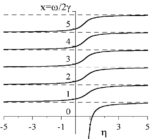
Figure 1: Particle lower energy levels in dependence on the parameter $\eta_{+}=\frac{\Gamma\left(\mu\right)}{\Gamma\left(1-\mu\right)}\left(\frac{\gamma}{2M^{2}}\right)^{1-\mu}\tan\left(\frac{\pi}{4}+\frac{\Theta}{2}\right)$

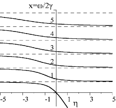
Figure 2: Antiparticle lower energy levels in dependence on the parameter $\eta_{-}=\frac{\Gamma\left(\mu\right)}{\Gamma\left(1-\mu\right)}\left(\frac{\gamma}{2M^{2}}\right)^{-\mu}\tan\left(\frac{\pi}{4}+\frac{\Theta}{2}\right)$

We can see that $\delta x_{m}=x_{m+1}\left(\eta\right)-x_{m}\left(\eta\right)\rightarrow 1$ with increasing $m$. It follows from the equation (79) that

$$\delta x_{m}-1=\pi^{-1}\left\{\cot\left(\pi x_{m}\right)-\cot\left[\pi\left(x_{m}-\mu\right)\right]\right\}^{-1}\left(\frac{1-\mu}{x_{m}}-\delta Q\right),\;m\gg 1\,,$$ (83)

where $\delta Q=\left.\frac{d}{dx}\ln Q(x)\right|_{x=x_{m}}\leq 1/x_{m}\,$. The curve $x_{5}\left(\eta\right)$ can give an idea about the behavior of the functions $x_{m}\left(\eta\right)$ for large $m\,$.

In the sequel, we discuss some limiting cases.

We first consider the weak fields $B$ for which $\gamma/M^{2}\ll 1$ and the nonrelativistic electron energies, $x_{m}\left(\eta\right)\gamma/M^{2}\ll 1$. Here, the functions $\,{}_{\pm}x\left(\eta\right)$ change significantly in the neighborhood of $\eta=0$ only. Beyond the neighborhood of $\eta=0,$ the functions $\,{}_{\pm}x\left(\eta\right)$ take the values close to the corresponding asymptotic values given by (82).

In the ultrarelativistic case, $x_{m}\left(\eta\right)\gamma/M^{2}\gg 1$, the behavior of $x_{m}\left(\eta\right)$ qualitatively depends on $\mu\,$. One can distinguish the three cases: $0<\mu<1/2$, $\mu>1/2$, and $\mu=1/2$. If $0<\mu<1/2,$ then the interval near $\eta=0$ on which the functions change significantly narrows down with increasing $m$. If $\mu>1/2,$ then this interval expands with increasing $m$ . For $\mu=1/2$ and $-\frac{1}{2}<\left(\frac{1}{4}+\frac{\Theta}{2\pi}\right)<\frac{1}{2}$, we find the asymptotic representation

$$\,{}_{\varsigma}x_{m}\left(\eta\right)=m+\varsigma\left(\frac{1}{4}+\frac{\Theta}{2\pi}\right),{}\;m\gg 1\;.$$ (84)

We see that negative ${}_{\pm}x_{0}\left(\eta\right)$ exist only for $\eta>0$. This means that in the problem under consideration, there exist only one particle state and only one antiparticle state with energies $\left|\varepsilon\right|<M$ for $\pi/2<\Theta<3\pi/2$. The same situation was observed in the pure AB field case [11]. The minimal admissible negative $x_{0}\left(\eta\right)$ is defined by the condition $\varepsilon=0$. For the strong fields $B$ for which $\gamma/M^{2}\sim 1$, the quantity $x_{0}\left(\eta\right)$ is close to zero. Let $\Theta_{0}$ correspond to such an extension that admits $\varepsilon=0$. The value of $\Theta_{0}$ is defined by

$$\tan\left(\frac{\pi}{4}+\frac{\Theta_{0}}{2}\right)=-\frac{\Gamma(1-\mu)\Gamma(\mu+M^{2}/2\gamma)}{2^{\mu}\Gamma(\mu)\Gamma(1+M^{2}/2\gamma)}\left(\frac{M^{2}}{\gamma}\right)^{1-\mu}.$$ (85)

In the weak fields, $\gamma/M^{2}\ll 1$, $x_{0}\left(\eta\right)$ takes large absolute values, and the angle $\Theta_{0}$ is defined by

$$\tan\left(\frac{\pi}{4}+\frac{\Theta_{0}}{2}\right)=-\frac{\Gamma(1-\mu)}{2^{2\mu-1}\Gamma(\mu)}\,$$ (86)

and independent from the magnetic field. It follows from (85) that in the superstrong fields $B$ for which $\gamma/M^{2}\gg 1$, the angle $\Theta_{0}$ is also independent from the magnetic field.

In the weak magnetic fields, $\gamma/M^{2}\ll 1$, and for the nonrelativistic energies, $x_{0}\gamma/M^{2}\ll 1$, we obtain the relations

$$\,{}_{+}x_{0}\left(\eta\right)=-\left(2/\eta\right)^{1/\left(1-\mu\right)}\,,$$ (87)

$$\,{}_{-}x_{0}\left(\eta\right)=-\left(\eta M^{2}/\gamma\right)^{1/\mu}\,$$ (88)

that are valid if $\eta$ in (87) is small and $\eta M^{2}/\gamma\gg 1$ in (88).

We now consider the particular case $\Theta=-\pi/2.$ It follows from (68) that for$\ B>0$, there exists ${}_{-}\varepsilon=-M$. The energies $\left|\varepsilon\right|>M$ are defined by the poles of $\Gamma(1-x)$ or $\Gamma(1-\mu-x)$ for $B>0$ or $B<0$, respectively. The spectrum $\varepsilon$ coincides with the one defined by Eqs. (176) and (38) for $\psi^{I}$. Moreover, using the relation (156), we can see that the spinors $\psi_{\omega}(r)$ coincide with $\psi^{I}$ up to a normalization constant,

$$\psi_{\omega}\left(r\right)\propto\psi^{I}\left(r\right)\;\mathrm{for\;}\Theta=-\pi/2\,.$$ (89)

In the case $\Theta=\pi/2$, we have the following picture: It follows from (68) that for $B<0$, there exists ${}_{+}\varepsilon=M$. The energies $\left|\varepsilon\right|>M$ are defined by the poles of $\Gamma(\mu-x)$ or $\Gamma(1-x)$ for $B>0$ or $B<0$, respectively. The spectrum $\varepsilon$ coincides with the one given by Eqs. (176) and (38) for $\psi^{II}$. It follows from (156) that the spinor $\psi_{\omega}(r)$ coincides with $\psi^{II}$ up to a normalization constant,

$$\psi_{\omega}(r)\propto\psi^{II}\left(r\right)\;\mathrm{for\;}\Theta=\pi/2\,.$$ (90)

Using the results for $B<0$, which are presented in Appendix B, we can conclude that the spectrum asymmetry holds for the spinning particles in the magnetic-solenoid field. There is a relation between the three-dimensional chiral anomaly and the fermion zero modes in a uniform magnetic field [39] (for review, see [40, 41]). We see that the effect also holds in the presence of the AB potential.

The spectrum asymmetry is known in 2+1 QED with the uniform magnetic field. In the uniform magnetic field, the states with $\omega=0$ for $l\neq 0$ are observed if sgn$l=-\mathrm{sgn}B$ (for the antiparticle if $B>0$ and for the particle if $B<0$). The spectrum changes mirror-like with the change of the sign of the magnetic field. We see that for $l\neq 0$, the spectrum properties in the magnetic-solenoid field is similar to the spectrum properties in the uniform magnetic field. The presence of the AB potential is especially essential for the states with $l=0$ where the particle penetrates the solenoid.

The spectra in $3+1$ dimensions can be obtained from the results in $2+1$ dimensions. Namely, we use the fact that the solutions $\psi_{\varepsilon,1}(x_{\perp})$ in $3+1$ dimensions are obtained from the solutions $\psi_{\varepsilon}^{(1)}(x_{\perp})$ in $2+1$ dimensions. Therefore, the spectra in $3+1$ dimensions are obtained from the results in $2+1$ dimensions by substituting $M$ by $\widetilde{M}$ and using the relation (55). As a consequence, we obtain an additional interpretation of Figs. 1 and 2. In particular, Fig.1 shows the lower energy levels for particles with spin $s=1$, and Fig. 2 shows the lower energy levels for particles with spin $s=-1$.

4 Solenoid regularization

4.1 Spinning particle case

We can introduce the AB field as a limiting case of a finite-radius solenoid field (the regularized AB field), which allows fixing the extension parameters. This approach to the pure AB field was first proposed by Hagen [12]. In what follows, we consider the problem in the presence of a uniform magnetic field. For this, we have to study the solutions of the Dirac equation (1) with the combination of a finite-radius solenoid field and a collinear uniform magnetic field.

Let the solenoid have a radius $R$. We assume that inside the solenoid, there is an axially symmetric magnetic field $B^{in}(r)$ that creates the flux $\Phi=\left(l_{0}+\mu\right)\Phi_{0},\;\Phi_{0}=2\pi/e$, such that $e\int_{0}^{R}B^{in}\left(r\right)rdr=l_{0}+\mu$, and outside the solenoid ($r>R$), the field $B^{in}(r)$ vanishes.. The function $B^{in}(r)$ is arbitrary but such that the integrals in the functions $\vartheta\left(x\right)\;$and $b\left(x\right)$ in (99) are convergent. We take the potentials of the field $B^{in}(r)$ in the form

$$eA_{1}^{in}=\vartheta\left(x\right)\frac{\sin\varphi}{Rx},\;eA_{2}=-\vartheta\left(x\right)\frac{\cos\varphi}{Rx}\,,$$ (91)

where

$$\;\vartheta\left(x\right)=\int_{0}^{x}f\left(x^{\prime}\right)x^{\prime}dx^{\prime},\;f(x)=R^{2}eB^{in}(xR),\;x=r/R\;.$$

The potentials of the uniform magnetic field are

$$A_{0}=0,\;A_{1}=A\left(r\right)\frac{\sin\varphi}{r},\;A_{2}=-A\left(r\right)\frac{\cos\varphi}{r}\;,\;\;A\left(r\right)=Br^{2}/2\;.$$ (92)

Outside the solenoid, the potentials have form (3).

We analyze the solutions of the Dirac equation in the field defined above . For this, we have to solve the equation inside and outside the solenoid and continuously sew the corresponding solutions. We call the corresponding Dirac spinors the respective inside and outside solutions.

We first study the problem in $2+1$ dimensions. We require that the solutions be square integrable and regular as $r\rightarrow 0$. In the same way as in Sec. 2, we obtain that the inside radial spinors $\psi_{\omega,l}^{in}(r)$ ($r\leq R$) satisfy the equation

$$h^{in}\psi_{\omega,l}^{in}\left(r\right)=\varepsilon\psi_{\omega,l}^{in}\left(r\right),\;\;h^{in}=\Pi^{in}+\sigma^{3}M\;,$$

where

$$\Pi^{in}=-\frac{i}{R}\left\{\partial_{x}+\frac{\sigma^{3}}{x}\left[l-l_{0}-\frac{1}{2}\left(1-\sigma^{3}\right)+\vartheta\left(x\right)+\xi\rho_{R}x^{2}\right]\right\}\sigma^{1},\;\rho_{R}=\gamma R^{2}/2\;.$$ (93)

We require that the functions $\psi_{\omega,l}^{in}\left(r\right)$ be square integrable on the interval $\left(0,R\right)$. For $\omega=0$ ($\left|\varepsilon\right|=M$), the solutions are

$${}_{+}\psi_{0,l}^{in}(r) = \phi_{0,l,1}^{in}(x)\upsilon_{1}\;,{}\;l-l_{0}\geq 1\;,$$

$${}_{-}\psi_{0,l}^{in}(r) = \phi_{0,l,-1}^{in}(x)\upsilon_{-1}\;,{}\;l-l_{0}\leq 0\;,$$

$$\phi_{0,l,\sigma}^{in}(x) = cx^{|\eta|}\exp\left\{\sigma\int_{0}^{x}\tilde{x}^{-1}\left(\vartheta(\tilde{x})+\xi\rho_{R}\tilde{x}^{2}\right)d\tilde{x}\right\},\;\eta=l-l_{0}-\left(1+\sigma\right)/2\;,$$ (94)

where $c$ is an arbitrary constant. For $\omega\neq 0$, we represent the spinors in the form

$$\psi_{\omega,l}^{in}\left(r\right)=\left(\begin{array}[]{c}\psi_{1}^{in}(r)\\ \psi_{2}^{in}(r)\end{array}\right)=\left[\sigma^{3}\left(\varepsilon-\Pi^{in}\right)+M\right]\left[c_{1}\phi_{l,1}^{in}(x)\upsilon_{1}+ic_{-1}\phi_{l,-1}^{in}(x)\upsilon_{-1}\right]\,,$$

where $c_{\sigma}$ are arbitrary constants. The functions $\phi_{l,\sigma}^{in}\left(x\right)$ satisfy the equation

$$\left[\frac{1}{x}\frac{\partial}{\partial x}x\frac{\partial}{\partial x}-\frac{1}{x^{2}}\left(\eta+\vartheta\left(x\right)+\xi\rho_{R}x^{2}\right)^{2}+\omega R^{2}-\sigma\left(f\left(x\right)+2\xi\rho_{R}\right)\right]\phi_{l,\sigma}^{in}\left(x\right)=0$$ (95)

and must be regular at $r=0$ in order to satisfy the square integrability condition for $\psi_{\omega,l}^{in}\left(r\right)$. Our prime interest is in the limiting case $R\rightarrow 0$. For our purposes, it is enough to use the approximation $\rho_{R}\ll 1$, $\omega R^{2}\ll 1$. Rejecting the terms proportional to $R^{2}$ in (93) and (95), we find that solutions of Eq. (95) are

$$\phi_{l,\sigma}^{in}\left(x\right)=\left\{\begin{array}[]{c}cx^{|\eta|}e^{\sigma b(x)},\;\sigma\eta\geq 0\,,\\ cx^{-|\eta|}e^{\sigma b(x)}\int_{0}^{x}d\tilde{x}\tilde{x}^{2|\eta|-1}e^{-2\sigma b(\tilde{x})},\;\sigma\eta<0\,,\end{array}\right.$$ (98)

$$b(x)=\int_{0}^{x}d\tilde{x}\tilde{x}^{-1}\vartheta(\tilde{x})\,.$$ (99)

The outside solutions ($r\geq R$) satisfy the equation

$$h\psi_{\omega,l}^{out}\left(r\right)=\varepsilon\psi_{\omega,l}^{out}\left(r\right)$$ (100)

and must be square integrable on the interval $\left(R,\infty\right)$. Here, $h$ is defined by Eqs. (10) and (11). The general form of the outside solutions is

$$\psi_{\omega,l}^{out}\left(r\right)=\left[\sigma^{3}\left(\varepsilon-\Pi\right)+M\right]\left(c_{1}\phi_{l,1}^{out}(r)\upsilon_{1}+ic_{-1}\phi_{l,-1}^{out}(r)\upsilon_{-1}\right)\,,$$

$$\phi_{l,\sigma}^{out}\left(r\right)=\psi_{\lambda,\alpha}\left(\rho\right)\;,\alpha=l+\mu-\left(1+\sigma\right)/2,\;2\lambda=\omega/\gamma-\xi\left(l+\mu-\left(1-\sigma\right)/2\right)\,.$$ (101)

The solutions $\psi_{\omega,l}^{out}\left(r\right)$ and $\psi_{\omega,l}^{in}\left(r\right)$ must be sewed continuously at $r=R$,

$$\psi^{out}\left(R\right)=\psi^{in}\left(R\right),$$ (102)

and must satisfy the normalization condition

$$N_{\omega,l}^{in}+N_{\omega,l}^{out}=1\,,$$

$$N_{\omega,l}^{in} = \int_{0}^{R}\left(\psi_{\omega,l}^{in}(r)\right)^{\dagger}\psi_{\omega,l}^{in}(r)rdr\;,\;\;N_{\omega,l}^{out}=\int_{R}^{\infty}\left(\psi_{\omega,l}^{out}(r)\right)^{\dagger}\psi_{\omega,l}^{out}(r)rdr\,.$$ (103)

We can treat the AB field as a limiting case of the finite-radius solenoid field if

$$\lim_{\rho_{R}\rightarrow 0}N_{\omega,l}^{in}=0\,.$$ (104)

We can realize the sewing condition (102) imposing the following conditions on the functions $\phi_{l,\sigma}^{in}\left(r\right)$ and $\phi_{l,\sigma}^{out}\left(r\right)$ at $r=R$:

$$\phi\left(R-\epsilon\right)=\phi\left(R+\epsilon\right),\;\frac{d}{dr}\phi\left(R-\epsilon\right)=\frac{d}{dr}\phi\left(R+\epsilon\right)\,.$$ (105)

It is convenient to use the representation (156) for $\psi_{\lambda,\alpha}\left(\rho\right)$ in (101).The functions $\phi_{l,\sigma}^{out}\left(r\right)$ then are

$$\phi_{l,\sigma}^{out}\left(r\right)=a_{\sigma}I_{n_{\sigma},m_{\sigma}}\left(\rho\right)+b_{\sigma}I_{m_{\sigma},n_{\sigma}}\left(\rho\right),\;n_{\sigma}=\lambda-\frac{1-\alpha}{2},\;m_{\sigma}=\lambda-\frac{1+\alpha}{2}\,,$$

$$a_{\sigma}=K\sin n_{\sigma}\pi,\;b_{\sigma}=-K\sin m_{\sigma}\pi,\;K=\frac{\sqrt{\Gamma\left(1+n_{\sigma}\right)\Gamma\left(1+m_{\sigma}\right)}}{\sin\left(n_{\sigma}-m_{\sigma}\right)\pi}\,,$$ (106)

where $n_{\sigma}$, $m_{\sigma}$ are real numbers.

Using (105), we can find the coefficients $a_{\sigma},\;b_{\sigma}$: for the case $l-l_{0}\leq 0$,

$$a_{1}=\rho_{R}^{-\left(l+\mu-1\right)/2}c\tilde{a}_{1},{}\;b_{1}=\rho_{R}^{\left(l+\mu-1\right)/2}c\tilde{b}_{1}\,,$$ (107)

$$a_{-1}=\rho_{R}^{-\left(l+\mu\right)/2+1}c\tilde{a}_{-1},{}\;b_{-1}=\rho_{R}^{\left(l+\mu\right)/2}c\tilde{b}_{-1}\,,$$ (108)

whereas for the case $l-l_{0}>0$,

$$a_{1}=\rho_{R}^{-\left(l+\mu-1\right)/2}c^{\prime}\tilde{a}_{1}^{\prime},{}\;b_{1}=\rho_{R}^{\left(l+\mu-1\right)/2+1}c^{\prime}\tilde{b}_{1}^{\prime}\,,$$ (109)

$$a_{-1}=\rho_{R}^{-\left(l+\mu\right)/2}c^{\prime}\tilde{a}_{-1}^{\prime},{}\;b_{-1}=\rho_{R}^{\left(l+\mu\right)/2}c^{\prime}\tilde{b}_{-1}^{\prime}\,,$$ (110)

where the non-vanishing coefficients $\tilde{a}$, $\tilde{b}$, $\tilde{a}^{\prime}$, $\tilde{b}^{\prime}$ are independent from $\rho_{R}$ and the coefficients $c$ and $c^{\prime}$ are normalization factors which depend on $\rho_{R}$.

Calculating the normalization factors, in the limit $R\rightarrow 0$, we obtain

$$a_{1} = \mathrm{const}\neq 0,\;b_{1}=0,\;a_{-1}=\;b_{-1}=0,\;l\geq 1\,,$$

$$a_{1} = 0,\;b_{1}=\mathrm{const}\neq 0,\;a_{-1}=\;b_{-1}=0,\;l\leq 0$$

for $l-l_{0}\leq 0$ and

$$a_{1} = b_{1}=0,\;a_{-1}=\mathrm{const}\neq 0,\;b_{-1}=0,\;l\geq 0\,,$$

$$a_{1} = b_{1}=0,\;a_{-1}=0,\;b_{-1}=\mathrm{const}\neq 0,\;l\leq-1$$

for $l-l_{0}>0$. For $l=0$, the value of the coefficients is defined by sgn$\Phi$. We can verify that the condition (104) is satisfied.

We thus obtain that for any sign of $B$, the solutions are expressed via Laguerre polynomials (38). In particular, for $l=0$, we find that the solutions $\psi_{\omega,0}^{out}\left(r\right)$ coincide with either $\psi_{m}^{I}\left(r\right)$ or $\psi_{m}^{II}\left(r\right)$ in accordance with $\mathrm{sgn}\left(\Phi\right)$,

$$\psi_{\omega,0}^{out}\left(r\right)=\left\{\begin{array}[]{c}\psi_{m}^{I}\left(r\right),\;\mathrm{sgn}\left(\Phi\right)=+1\\ \psi_{m}^{II}\left(r\right),\;\mathrm{sgn}\left(\Phi\right)=-1\end{array}\right.\,.$$ (111)

In Sec. 3, we have found the relation between the extension parameter values and the types of solutions in the critical subspace $l=0$ (89), (90). We are now in a position to refine this relation. Namely, if we introduce the AB field as the field of the zero-radius limit for the finite-radius solenoid , then the extension parameter $\Theta$ is fixed to be $\Theta=-\mathrm{sgn}\left(\Phi\right)\pi/2$. In addition, this way of introducing the AB field implies no additional interaction in the solenoid core.

To solve the problem in $3+1$ dimensions, we use the results in $2+1$ dimensions presented above. In the limit $R\rightarrow 0$, the solutions in the critical subspace are

$$\Psi_{s}^{out}\left(x_{\bot}\right)=N\left(\begin{array}[]{c}\left[1+\left(p^{3}+s\widetilde{M}\right)/M\right]g_{0}\left(\varphi\right)\psi_{\omega,l}^{out}\left(r\right)\\ \left[-1+\left(p^{3}+s\widetilde{M}\right)/M\right]g_{0}\left(\varphi\right)\psi_{\omega,l}^{out}\left(r\right)\end{array}\right)\,,$$ (112)

where the functions $g_{0}\left(\varphi\right)$, $\psi_{\omega,l}^{out}\left(r\right)$ are defined in (9) and (111), (38), respectively. The values of the extension parameters in $3+1$ dimensions are specified to be

$$\Theta_{+1}=\Theta_{-1}=-\frac{\pi}{2}\mathrm{sgn\,}\Phi\,.$$ (113)

The interpretation of other possible $\Theta$’s via the limiting process for other regularized potentials is not reached so far.

4.2 Spinless particle case

For completeness, let us consider the regularization problem in the spinless particle case. For this case the Klein-Gordon equation with the magnetic-solenoid field is, in fact, reduced to the eigenvalue problem for the nonrelativistic two-dimensional Hamiltonian. Therefore, the self-adjoint extension problem as well as the solenoid regularization problem is similar for the relativistic and nonrelativistic case.

From the classical paper [35] on, the AB effect in the spinless case was always associated with the radial functions regular at $r=0$. However, the linkage between these kind of boundary conditions and a regularizing solenoid is an interesting important problem. The aim of this subsection is just to study this problem.

One ought to say self-adjoint extensions of the nonrelativistic spinless Hamiltonian with the AB field were studied in several articles [6, 7, 8, 9]. The case of the magnetic-solenoid field was considered in [34] where the most general four-parameter family of admissible boundary conditions was obtained. The solenoid regularization with some particular distributions of the magnetic field inside the solenoid was studied in [6, 12]. As we know, the regularization problem with the arbitrary field inside the solenoid was not solved.

Unlike the Dirac equation, the Klein-Gordon equation was not solved explicitly for the arbitrary field inside the regularizing solenoid. However, one can obtain some properties of the corresponding solutions without the explicit solving the Klein-Gordon equation. Thus, we can demonstrate that for the arbitrary field inside the solenoid, the lifting of the regularization ($R\rightarrow 0$) corresponds to regular radial functions only.

To do that we use the above formulated in the Dirac case method. Solutions of the Klein-Gordon equation with a given energy $\varepsilon$ and angular momentum $l-l_{0}$ have the form

$$\phi\left(x\right)=Ne\,^{i\varepsilon x^{0}}e^{i\left(l-l_{0}\right)\varphi}\phi\left(r\right)\,.$$

We find the radial function $\phi\left(r\right)$ sewing solutions inside and outside the solenoid.

The outside solutions have the form [4],

$$\phi^{out}\left(r\right)=\psi_{\lambda,\alpha/2}\left(\rho\right)=\rho^{-1/2}W_{\lambda,\alpha/2}\left(\rho\right),\;2\lambda=\omega/\gamma-\xi\alpha,\;\alpha=l+\mu\,,$$ (114)

where, as before, $\omega=\varepsilon^{2}-M^{2}$. The critical subspace is defined by $l=0,-1$. The inside solutions satisfy the equation (95) where one has to set $\sigma=0$. The approximation $\rho_{R}\ll 1$ and $\omega R^{2}\ll 1$ can be applied in this case as well. Therefore, we arrive to the following equation for the inside solutions,

$$\left[\frac{d^{2}}{dx^{2}}+\frac{1}{x}\frac{d}{dx}-\frac{1}{x^{2}}\left(\eta+\vartheta\left(x\right)\right)^{2}\right]\phi^{in}\left(x\right)=0\,,$$ (115)

where $0\leq x\leq 1$. We are looking for solutions $\phi^{in}\left(x\right)$ that are regular at $x=0$. Applying the sewing conditions (105), we obtain

$$\alpha\phi_{in}\left(1\right)+\partial_{x}\phi^{in}\left(1\right)=2\alpha a\rho_{R}^{\alpha/2}\,,\;\alpha\phi_{in}\left(1\right)-\partial_{x}\phi^{in}\left(1\right)=2\alpha b\rho_{R}^{-\alpha/2}$$ (116)

in the lower order in $\rho_{R}$.

For our purposes it is important to demonstrate that the following condition holds true

$$\left|\alpha\right|\phi^{in}\left(1\right)+\partial_{x}\phi^{in}\left(1\right)\neq 0\,.$$ (117)

To this end, let us find solutions of equation (115) that are regular at $x=0$. The function $\vartheta\left(x\right)$ is analytic on the interval $0\leq x\leq 1$ as obeying the conditions listed in Sec. 4.1. Then (115) is the homogeneous ordinary differential equation with the regular singular point $x=0$. It is known from the general theory [36] that there exist solutions of (115) that can be represented in the form

$$\phi^{in}\left(x\right)=x^{\left|\eta\right|}\sum_{k=0}^{\infty}a_{k}x^{k}\,,$$ (118)

where $a_{0}$ is an arbitrary constant and the other coefficients are defined via recurrent relations. The series in (118) is absolutely and uniformly convergent for $0\leq x\leq 1$. Let us suppose now for simplicity that $f\left(x\right)$ does not change its sign for $0\leq x\leq 1$. Then we represent $\phi^{in}\left(x\right)$ in the form

$$\phi_{in}\left(x\right)=\left\{\begin{array}[]{c}x^{\left|\eta\right|}e^{-\left|b\left(x\right)\right|}\varphi^{\left(-\right)}\left(x\right),\;\mathrm{sgn}\left(f\right)\eta\leq 0\\ x^{-\left|\eta\right|}e^{-\left|b\left(x\right)\right|}\varphi^{\left(+\right)}\left(x\right),\;\mathrm{sgn}\left(f\right)\eta>0\end{array}\right.,$$ (119)

where the functions $\varphi^{\left(\pm\right)}\left(x\right)$ obey the equation

$$H^{\left(\pm\right)}\varphi^{\left(\pm\right)}=0\,,\;H^{\left(\pm\right)}=H_{0}^{\left(\pm\right)}-\left|f\left(x\right)\right|\,,\;H_{0}^{\left(\pm\right)}=\frac{d^{2}}{dx^{2}}+\left(1\mp 2\left|\eta\right|-2\left|\vartheta\left(x\right)\right|\right)\frac{1}{x}\frac{d}{dx}$$ (120)

and the conditions

$$\varphi^{\left(-\right)}\left(0\right)=1,\;\left.x^{-2\left|\eta\right|}\varphi^{\left(+\right)}\left(x\right)\right|_{x=0}=1\,.$$ (121)

It is convenient to introduce into the consideration the retarded propagator $G_{ret}^{\left(\pm\right)}\left(x,y\right)$ obeying the equation

$$H_{0}^{\left(\pm\right)}G_{ret}^{\left(\pm\right)}\left(x,y\right)=\delta\left(x-y\right)\,.$$

It can be represented as $G_{ret}^{\left(\pm\right)}\left(x,y\right)=\theta\left(x-y\right)G^{\left(\pm\right)}\left(x,y\right)$ where the functions $G^{\left(\pm\right)}$ obey the conditions

$$G^{\left(\pm\right)}\left(x,x\right)=0,\;\left.\frac{\partial}{\partial x}G^{\left(\pm\right)}\left(x,y\right)\right|_{x=y}=1\,,$$

and can be found explicitly in the case under consideration,

$$G^{\left(\pm\right)}\left(x,y\right)=\int_{y}^{x}\left(\frac{\widetilde{x}}{y}\right)^{\pm 2\left|\eta\right|-1}\exp\left\{2\left|b\left(\widetilde{x}\right)\right|-2\left|b\left(y\right)\right|\right\}d\widetilde{x}\,.$$ (122)

The differential equation (120) with the boundary conditions (121) is equivalent to the following integral equation,

$$\varphi^{\left(\pm\right)}\left(x\right)=\varphi_{0}^{\left(\pm\right)}\left(x\right)+\int_{0}^{x}G^{\left(\pm\right)}\left(x,y\right)\left|f\left(y\right)\right|\varphi^{\left(\pm\right)}\left(y\right)dy\,,$$ (123)

where

$$\varphi_{0}^{\left(-\right)}\left(x\right)=1,\;\varphi_{0}^{\left(+\right)}\left(x\right)=\int_{0}^{x}\widetilde{x}^{2\left|\eta\right|-1}e^{2\left|b\left(\widetilde{x}\right)\right|}d\widetilde{x}\,.$$

The solutions of the equation (123) can be found by iterations,

$$\varphi^{\left(\pm\right)}\left(x\right) = \sum_{k=0}^{\infty}Y_{k}^{\left(\pm\right)}\left(x\right)\,,\;$$

$$Y_{k}^{\left(\pm\right)}\left(x\right) = \int_{0}^{x}G^{\left(\pm\right)}\left(x,y\right)\left|f\left(y\right)\right|Y_{k-1}^{\left(\pm\right)}\left(y\right)dy,\;Y_{0}^{\left(\pm\right)}\left(x\right)=\varphi_{0}^{\left(\pm\right)}\left(x\right)\,.$$ (124)

Every member of the series (124) is positive. The series converges uniformly. Then, it implies $\varphi^{\left(\pm\right)}\left(x\right)>0$ and $\partial_{x}\varphi^{\left(\pm\right)}\left(x\right)>0$ for $x>0$. Therefore,

$$\phi^{in}\left(1\right)>0,\;\partial_{x}\phi^{in}\left(1\right)=-\mathrm{sgn}\left(f\right)\alpha\phi^{in}\left(1\right)+e^{-\left|b\left(1\right)\right|}\partial_{x}\varphi^{\left(\pm\right)}\left(1\right)\,.$$ (125)

If sgn$\left(f\right)\alpha<0,$ then $\partial_{x}\phi^{in}\left(1\right)>0$ and the condition (117) is satisfied. If sgn$\left(f\right)\alpha>0$, then it follows from (125) that

$$\left|\alpha\right|\phi^{in}\left(1\right)+\partial_{x}\phi^{in}\left(1\right)>0\,,$$

and the condition (117) is satisfied as well. The obtained result can be extended to the function $f\left(x\right)$ alternating in sign. In this case the interval $\left[0,1\right]$ can be divided into subintervals on which $f\left(x\right)$ does not change its sign. The solutions $\phi^{in}\left(x\right)$ can be found successively on each such a subinterval beginning from the point $x=0$.

Applying the normalization condition for the sewed solutions,

$$\int_{0}^{\rho_{R}}\left|\phi^{in}\right|^{2}d\rho+\int_{\rho_{R}}^{\infty}\left|\phi^{out}\right|^{2}d\rho=1\,,$$

we get

$$b=0\;\text{if}\;\alpha>0;\;a=0\;\text{if}\;\alpha<0$$ (126)

in the limit $R\rightarrow 0$. Thus, the only regular at $r=0$ solutions remain in the limit $R\rightarrow 0$. The conditions (126) also define the spectrum. Finally, it follows from (106) that in the limit $R\rightarrow 0$ the radial functions and the related spectrum has the form

$$\phi_{m,l}\left(r\right)=I_{m+\left|l+\mu\right|,m}\left(\rho\right)\,,\;\omega=\gamma\left(2m+\left|l+\mu\right|+\xi\left(l+\mu\right)+1\right)\,.$$ (127)

5 Reduced self-adjoint extension method

We here show that the general self-adjoint extension method can be significantly reduced for the radial Hamiltonian $h$ given by Eqs. (10), (11).

We recall that the problem is to define the formal matrix differential operator (10), (11) as a self-adjoint operator in the Hilbert space of two-spinors $\chi\left(r\right)$ square-integrable on the half-line $R_{+}=\{r\geq 0\}$ with the measure $rdr.$ It is convenient to pass to the standard measure $dr$ on $R_{+}$ with the substitution $\chi\left(r\right)=r^{-1/2}\Psi\left(r\right)\,.$ The radial Hamiltonian then becomes (we do not change the notation for the transformed Hamiltonian $h$)

$$h=\Pi+\sigma^{3}M\,,\;\;\Pi=\left(\begin{array}[]{cc}0&a_{\nu,B}\\ a_{-\nu,-B}&0\end{array}\right)\,,$$ (128)

where $\nu=\mu+l-1/2$ and the operator $a_{\nu,B}$: $L_{2}\rightarrow L_{2}$ is

$$a_{\nu,B}=-i\left(\partial_{r}+\frac{\nu}{r}+\frac{eBr}{2}\right)=-i\sigma_{-\nu,-B}\partial_{r}\sigma_{\nu,B}$$ (129)

with

$$\sigma_{\nu,B}=r^{\nu}\exp\left(\frac{eBr^{2}}{4}\right)\,,\;\sigma_{-\nu,-B}\sigma_{\nu,B}=1\,.$$

This $h$ (128) must be defined as a self-adjoint operator in the Hilbert space

$$\mathcal{H}=L_{2}\left(R_{+}\right)\oplus L_{2}\left(R_{+}\right)$$

of two-spinors

$$\Psi\left(r\right)=\left(\begin{array}[]{c}\psi^{1}\left(r\right)\\ \psi^{2}\left(r\right)\end{array}\right)$$

square integrable on $R_{+\,}$.

We first note that $\sigma^{3}M$ is a bounded self-adjoint operator in $\mathcal{H}.$ Therefore, the problem is equivalent to the problem of defining the apparently self-adjoint operator $\Pi$ (128) as a really self-adjoint operator in $\mathcal{H}:$ we must ensure the equality $\Pi=\Pi^{\dagger}$ by the proper choice of the domain

$$\mathcal{D}(\Pi)=\mathcal{D}(a_{-\nu,-B})\oplus\mathcal{D}(a_{\nu,B})\subset\mathcal{H}\,,$$

for any $\nu$ and $B$. The problem is thus, reduced to the problem of properly defining $a_{\nu,B}$ (129) as an operator in $L_{2}\left(R_{+}\right),$ i.e., defining $\mathcal{D}(a_{\nu,B})\subset L_{2}\left(R_{+}\right),$ together with $a_{-\nu,-B}\,$.

We canonically start with defining $\Pi$ as a symmetric operator in $\mathcal{H}$ by taking the initial domain to be $\mathcal{D}(\Pi)=D\oplus D$, such that the both $a_{\nu,B}$ and $a_{-\nu,-B}$ are initially defined on $D\subset L_{2}\left(R_{+}\right),$ where $D$ is the linear space of $C^{\infty}$-functions with compact support. We note that $\Pi$ is densely defined because $\overline{D}\subset L_{2}\left(R_{+}\right)$ and symmetric, $\Pi\subseteq\Pi^{\dagger}$, which is simply verified by integration by parts.

The next step is the evaluation of its adjoint  $\Pi^{\dagger}.$ It is evident that

$$\,\Pi^{\dagger}=\left(\begin{array}[]{cc}0&a_{-\nu,-B}^{\dagger}\\ a_{\nu,B}^{\dagger}&0\end{array}\right)\,,\;\;\mathcal{D}(\,\Pi^{\dagger})=\mathcal{D}(a_{\nu,B}^{\dagger})\oplus\mathcal{D}(a_{-\nu,-B}^{\dagger})\,,$$ (130)

for any $\nu$ and $B.$ Because $a_{\nu,B}$ is a simple differential operator in $L_{2}\left(R_{+}\right),$ its adjoint $a_{\nu,B}^{\dagger}$ is evaluated simply (by the standard method for differential operators in $L_{2}\left(R_{+}\right)$): its form is

$$a_{\nu,B}^{\dagger}=-i\sigma_{\nu,B}\,\partial_{r}\sigma_{-\nu,-B}$$ (131)

(it coincides with $a_{-\nu,-B}$ (129)), and its domain is

$$\mathcal{D}(a_{\nu,B}^{\dagger})=\{_{\ast}\psi_{\nu,B}\left(r\right)\}\,,$$ (132)

where ${}_{\ast}\psi_{\nu,B}\left(r\right)$ are absolutely continuous (inside $R_{+}$) square integrable functions allowing the representation

$${}_{\ast}\psi_{\nu,B}\left(r\right)=i\sigma_{\nu,B}\left(r\right)\left[\int_{r_{0}}^{r}d\xi\,\sigma_{-\nu,-B}\left(\xi\right)_{\ast}\phi_{\nu,B}\left(\xi\right)+c_{\nu,B}\right]\,.$$ (133)

Here, ${}_{\ast}\phi_{\nu,B}=a_{\nu,B}^{\dagger}\,{}_{\ast}\psi_{\nu,B},$ the image of $a_{\nu,B}^{\dagger}$ on ${}_{\ast}\psi_{\nu,B}$ , is square integrable, ${}_{\ast}\phi_{\nu,B}\in L_{2}\left(R_{+}\right);\;c_{\nu,B}$ is a constant restricted by the requirement that ${}_{\ast}\psi_{\nu,B}\in L_{2}\left(R_{+}\right);\;r_{0}\geq 0$ is chosen appropriately depending on the value of $\nu$ and the sign of $B.$ Of course, the same is true for $a_{-\nu,-B}^{+}:$ we must simply make the substitutions $\nu\rightleftarrows-\nu,\;B\rightleftarrows-B$ in (131-133).

At this point, we depart from the general procedure used in Sec. 3: then finding the deficiency subspaces and etc. Instead, we determine the ”asymmetry” of  $\Pi^{\dagger}$ evaluating the difference

$$\Delta=\left({}_{\ast}\Psi^{\prime},\,\Pi^{\dagger}{}_{\ast}\Psi\right)-\left(\,\Pi^{\dagger}{}_{\ast}\Psi^{\prime},_{\ast}\Psi\right)$$ (134)

for any ${}_{\ast}\Psi$ and${}_{\ast}\Psi^{\prime}$ belonging to $\mathcal{D}($ $\Pi^{\dagger}).$ Using the form of ${}_{\ast}\Psi\in\mathcal{D}($ $\Pi^{\dagger}),$ see (130), (132), (133),

$${}_{\ast}\Psi\left(r\right)=\left(\begin{array}[]{c}{}_{\ast}\psi_{\nu,B}^{1}\left(r\right)\\ {}_{\ast}\psi_{-\nu,-B}^{2}\left(r\right)\end{array}\right)$$ (135)

and the form (130) of  $\Pi^{\dagger},$ we obtain (we here omit the subscripts $\ast$ and $B$ as irrelevant, which becomes clear below)

$$\Delta=\int_{0}^{\infty}dr\left[\overline{\psi_{\nu}^{\prime 1}\left(r\right)\,}a_{-\nu}^{\dagger}\psi_{-\nu}^{2}\left(r\right)+\overline{\psi_{-\nu}^{\prime 2}\left(r\right)\,}a_{\nu}^{\dagger}\psi_{\nu}^{1}\left(r\right)\right]$$

$$-\int_{0}^{\infty}dr\left[\overline{a_{-\nu}^{\dagger}\psi_{-\nu}^{\prime 2}\left(r\right)}\,\psi_{\nu}^{1}\left(r\right)+\overline{a_{\nu}^{\dagger}\psi_{\nu}^{\prime 1}\left(r\right)\,}\psi_{-\nu}^{2}\left(r\right)\right]\,.$$

Integrating by parts in the first integral, we find

$$\Delta=-i\left.\left[\overline{\psi_{\nu}^{\prime 1}\left(r\right)}\psi_{-\nu}^{2}\left(r\right)+\overline{\psi_{-\nu}^{\prime 2}\left(r\right)}\psi_{\nu}^{1}\left(r\right)\right]\right|_{0}^{\infty}\,,$$

i.e., $\Delta$ is determined by the asymptotic behavior of ${}_{\ast}\Psi$ (135) at the boundaries, as $r\rightarrow\infty$ and $r\rightarrow 0.$ The asymptotic behavior for ${}_{\ast}\psi_{\nu,B}\left(r\right)$ and ${}_{\ast}\psi_{-\nu,-B}\left(r\right)$ can be estimated using the representation (133) with the appropriate choice of $r_{0}$ and estimating the integral term in (133) via the Cauchy-Bounjakowsky inequality.

For example, we estimate the behavior of ${}_{\ast}\psi_{\nu,B}\left(r\right)$ at infinity, as $r\rightarrow\infty,$ in the case $B>0.$ In this case, it is convenient to take $r_{0}=\infty,$ such that

$${}_{\ast}\psi_{\nu,B}\left(r\right)=i\sigma_{\nu,B}\left(r\right)\left[-\int_{r}^{\infty}d\xi\,\sigma_{-\nu,-B}\left(\xi\right)_{\ast}\phi_{\nu,B}\left(\xi\right)+c_{\nu,B}\right]\,.$$ (136)

The Cauchy-Bounjakowsky inequality yields

$$\left|\int_{r}^{\infty}d\xi\xi^{-\nu}\exp\left(-\frac{eB\xi^{2}}{4}\right)\right|\leq\left[\int_{r}^{\infty}d\xi\,\xi^{-2\nu}\exp\left(-\frac{eB\xi^{2}}{4}\right)\,_{\ast}\phi_{\nu,B}\left(\xi\right)\right]^{1/2}$$

$$\,\times\left[\int_{r}^{\infty}d\xi\left|{}_{\ast}\phi_{\nu,B}\left(\xi\right)\right|^{2}\right]^{1/2}=\frac{r^{-\nu-1/2}}{eB}\exp\left(-\frac{eBr^{2}}{4}\right)\left(1+O\left(\frac{1}{r}\right)\right)\epsilon\left(r\right)\,,$$ (137)

where $\epsilon\left(r\right)\rightarrow 0$ as $r\rightarrow\infty.$ It follows from (137) and the condition ${}_{\ast}\psi_{\nu,B}\in L_{2}\left(R_{+}\right)$ that $c_{\nu,B}$ in (136) must be zero and, consequently, ${}_{\ast}\psi_{\nu,B}\left(r\right)$ vanishes as $r\rightarrow\infty,$ faster than $r^{-1/2},$ independently from $\nu.$ The same is true for $B<0,$ which is established via the Cauchy-Bounjakowsky inequality with $r_{0}<\infty.$

The asymptotic estimates for ${}_{\ast}\psi_{\nu,B}\left(r\right)$ as $r\rightarrow 0$ depend on the value of $\nu.$ The result is:

$$\nu>\frac{1}{2} : \;\left|{}_{\ast}\psi_{\nu,B}\left(r\right)\right|<c_{\nu}r^{1/2}\,,$$

$$\nu=\frac{1}{2} : \;\left|{}_{\ast}\psi_{1/2,B}\left(r\right)\right|<c_{1/2}\,r^{1/2}\ln\frac{r}{r_{0}}\,,$$

$$\nu\leq-\frac{1}{2} : \;{}_{\ast}\psi_{\nu,B}\left(r\right)=o\left(r^{1/2}\right)\,,$$

$$-\frac{1}{2}<\nu<\frac{1}{2} : \;{}_{\ast}\psi_{\nu,B}\left(r\right)=c_{\nu,B}\,\left(rM\right)^{\nu}+o\left(r^{1/2}\right)\,,$$

independently from $B;$ the factor $M$ is introduced by the dimensional reasons.

We conclude that for $\left|\nu\right|\geq 1/2\,,$ the two-spinors ${}_{\ast}\Psi\left(r\right)$ (135) vanish both at infinity and at the origin, whereas for $\left|\nu\right|<1/2\,,\;$the two-spinors ${}_{\ast}\Psi\left(r\right)$ vanish at infinity, but are generally singular as $r\rightarrow 0:$

$${}_{\ast}\Psi\left(r\right)=\left(\begin{array}[]{c}c_{\nu,B}^{1}\,\left(rM\right)^{\nu}\\ c_{-\nu,-B}^{2}\,\left(rM\right)^{-\nu}\end{array}\right)+o\left(r^{1/2}\right)\,,$$ (138)

where $c^{1,2}$ are arbitrary constants. With this estimates in hand, we find

$$\Delta=\left\{\begin{array}[]{c}0\,,\;\left|\nu\right|\geq 1/2\\ i\left[c_{\nu}^{\prime 1}c_{-\nu}^{2}+c_{-\nu}^{\prime 2}c_{\nu}^{1}\right]\,,\;\left|\nu\right|<1/2\end{array}\right.,$$ (139)

independently of $B$ (we therefore omit the subscripts $\ast$ and $B$ as irrelevant).

We thus find that if $\left|\nu\right|\geq 1/2\,,$ i.e., if $l\neq 0$ or $l=0$ and $\mu=0$, the operator $\Pi^{\dagger}$ is symmetric, $\Pi^{\dagger}\subseteq\left(\Pi^{\dagger}\right)^{\dagger}$, and therefore self-adjoint, $\Pi^{\dagger}=\left(\Pi^{\dagger}\right)^{\dagger}$: it is sufficient to take the inverse inclusion $\left(\Pi^{\dagger}\right)^{\dagger}\subseteq\Pi^{\dagger}$ into account, the standard relation for any symmetric operator (which is the consequence of the general relations $A\subseteq B\rightarrow B^{\dagger}\subseteq A^{\dagger}$ for any densely defined operators). Thus, $\Pi^{\dagger}$ is a self-adjoint extension of $\Pi$.

This implies that $\Pi$ is essentially self-adjoint, i.e., its closure $\overline{\Pi}$ is self-adjoint, $\overline{\Pi}=\overline{\Pi}^{\dagger}$, in addition $\overline{\Pi}=\Pi^{\dagger}$ and is a unique self-adjoint extension of $\Pi$. We recall the standard arguments. As is well known, $\overline{\Pi}=\left(\Pi^{\dagger}\right)^{\dagger}$ and $\overline{\Pi}^{\dagger}=\Pi^{\dagger}$. Using the established self-adjointness of $\Pi^{\dagger}$, $\Pi^{\dagger}=\left(\Pi^{\dagger}\right)^{\dagger}$, we obtain the chain of equalities $\overline{\Pi}=\left(\Pi^{\dagger}\right)^{\dagger}=\Pi^{\dagger}=\overline{\Pi}^{\dagger}$, which proves the first two assertions. There are no other self-adjoint extensions because any such extension $\Pi^{ext}=\left(\Pi^{ext}\right)^{\dagger}$ must satisfy the relation $\overline{\Pi}\subseteq\Pi^{ext}\subseteq\Pi^{\dagger}$, $\Pi^{ext}$ must be the extension of $\overline{\Pi}$ and the restriction of $\Pi^{\dagger}$, but because $\overline{\Pi}=\Pi^{\dagger}$, there are ”no place ” for another self-adjoint extension.

The situation is nontrivial in the case $\left|\nu\right|<1/2$, i.e. if $l=0$ and $\mu\neq 0$, where the operator $\Pi^{\dagger}$ is nonsymmetric, which implies that $\overline{\Pi}$ is only symmetric: $\overline{\Pi}=\left(\Pi^{\dagger}\right)^{\dagger}\subset\Pi^{\dagger}=\overline{\Pi}^{\dagger}$ is a strict inclusion. This relation allows finding $\overline{\Pi}$. The inclusion $\overline{\Pi}\subset\Pi^{\dagger}$ implies that $\mathcal{D}\left(\overline{\Pi}\right)\subset\mathcal{D}\left(\Pi^{\dagger}\right)$, i. e. $\Psi^{\prime}\in$ $\mathcal{D}\left(\overline{\Pi}\right)$ has the representations like (133) and (138),

$$\Psi^{\prime}\left(r\right)=\left(\begin{array}[]{c}c^{\prime 1}\left(rM\right)^{\nu}\\ c^{\prime 2}\left(rM\right)^{-\nu}\end{array}\right)+o\left(r^{1/2}\right),$$ (140)

and vanish at infinity. Then the equality $\overline{\Pi}=\left(\Pi^{\dagger}\right)^{\dagger}\subset\Pi^{\dagger}$ implies, by the definition of $\left(\Pi^{\dagger}\right)^{\dagger}$, that $\Psi^{\prime}\in\mathcal{D}\left(\overline{\Pi}\right)$ iff the difference $\Delta$ (134) vanishes for $\Psi^{\prime}\in\mathcal{D}\left(\overline{\Pi}\right)\subset\mathcal{D}\left(\Pi^{\dagger}\right)$ and any $\Psi\in\mathcal{D}\left(\Pi^{\dagger}\right)$. According to (139), this gives

$$\overline{c_{\nu}^{\prime 1}}c_{-\nu}^{2}+\overline{c_{-\nu}^{\prime 2}}c_{\nu}^{1}=0,\;\forall c_{\nu}^{1},\;c_{-\nu}^{2}\,,$$

whence $c_{\nu}^{\prime 1}=c_{-\nu}^{\prime 2}=0$. $\overline{\Pi}$ is thus defined as the restriction of $\Pi^{\dagger}$ to the domain $\mathcal{D}\left(\overline{\Pi}\right)$ of the functions belonging to $\mathcal{D}\left(\Pi^{\dagger}\right)$, but vanishing at the origin.

We must seek the self-adjoint extensions $\Pi^{ext}=\left(\Pi^{ext}\right)^{\dagger}$ of $\Pi$. These, as was said just before, ”must lie between” $\overline{\Pi}$ and $\Pi^{\dagger}$, $\overline{\Pi}\subset\Pi^{ext}=\left(\Pi^{ext}\right)^{\dagger}\subset\Pi^{\dagger}$. We start with finding the nontrivial (not coinciding with $\overline{\Pi}$) symmetric extensions $\Pi^{sym}$ of $\Pi$, $\overline{\Pi}\subset\Pi^{sym}\subseteq\left(\Pi^{sym}\right)^{\dagger}\subseteq\Pi^{\dagger}$ and then show that these $\Pi^{sym}$ solve the problem. The last inclusions allows repeating for $\Pi^{sym}$ the previous arguments for $\overline{\Pi}$ except that now the difference $\Delta$ (134) must vanish for any $\Psi$, $\Psi^{\prime}\in\mathcal{D}\left(\Pi^{sym}\right)\subset\mathcal{D}\left(\Pi^{\dagger}\right)$. According to (139) this gives the equation for $c_{\nu}^{1}$,$\;c_{-\nu}^{2}$ in $\Psi$ (138) and $c_{\nu}^{\prime 1}$, $c_{-\nu}^{\prime 2}$ in $\Psi^{\prime}$ (140),

$$\overline{c_{\nu}^{\prime 1}}c_{-\nu}^{2}+\overline{c_{-\nu}^{\prime 2}}c_{\nu}^{1}=0,$$ (141)

Of course, if $\Psi$, $\Psi^{\prime}\in\mathcal{D}\left(\overline{\Pi}\right)\subset\mathcal{D}\left(\Pi^{sym}\right)$, i.e. vanish at the origin, Eq. (141) holds. To satisfy (141) it is sufficient that only $\Psi$ or $\Psi^{\prime}$ belong to $\mathcal{D}\left(\overline{\Pi}\right)$. But $\mathcal{D}\left(\Pi^{sym}\right)$ must contain functions nonvanishing at the origin. Let $\Psi$ be such a function and, for example, let $c_{-\nu}^{2}\neq 0$. For $\Psi^{\prime}=\Psi$, Eq. (141) becomes

$$\overline{c_{\nu}^{1}}c_{-\nu}^{2}+\overline{c_{-\nu}^{2}}c_{\nu}^{1}=0,$$

whence

$$\frac{c_{\nu}^{1}}{c_{-\nu}^{2}}=-\frac{\overline{c_{\nu}^{1}}}{\overline{c_{-\nu}^{2}}}=i\,\Lambda,\;\,\Lambda\in\mathbb{R}.$$

Then for any $\Psi^{\prime}\in\mathcal{D}\left(\Pi^{sym}\right)$ nonvanishing at the origin and this fixed $\Psi$, Eq. (141) becomes

$$\overline{c_{\nu}^{\prime 1}}+i\,\Lambda\overline{c_{-\nu}^{\prime 2}}=0,$$

whence $c_{-\nu}^{\prime 2}\neq 0$ and $c_{\nu}^{\prime 1}/c_{-\nu}^{\prime 2}=i$ $\Lambda$, with the same  $\Lambda$ for all $\Psi\in\mathcal{D}\left(\Pi^{sym}\right)$ nonvanishing at the origin.

The case $c_{-\nu}^{2}=0$, $c_{\nu}^{1}\neq 0$ is considered similarly. It is formally covered by the case  $\Lambda=\pm\infty$, where  $\Lambda=+\infty$ and  $\Lambda=-\infty$ are equivalent (both simply mean $c_{-\nu}^{2}=0$, $c_{\nu}^{1}\neq 0$). We thus obtain the asymptotic boundary conditions

$$\Psi\left(r\right)=c\left(\begin{array}[]{c}i\,\Lambda\left(rM\right)^{\nu}\\ \left(rM\right)^{-\nu}\end{array}\right)+o\left(r^{1/2}\right)$$ (142)

at the origin as $r\rightarrow 0$, that define a one-parameter family $\left\{\Pi^{\,\Lambda}\right\}$ of all nontrivial symmetric extensions of $\Pi$.

It remains to show that these extensions $\Pi^{\,\Lambda}$ are really self-adjoint, $\Pi^{\,\Lambda}=\left(\Pi^{\,\Lambda}\right)^{\dagger}$. For this, it is necessary to evaluate $\left(\Pi^{\Lambda}\right)^{\dagger}$. Using the arguments similar to the previous ones, we conclude that $\Psi^{\prime}\in\mathcal{D}\left(\left(\Pi^{\,\Lambda}\right)^{\dagger}\right)$ iff the difference $\Delta$ (134) vanish for $\Psi^{\prime}\in\mathcal{D}\left(\left(\Pi^{\Lambda}\right)^{\dagger}\right)\subseteq\mathcal{D}\left(\Pi^{\dagger}\right)$ and any $\Psi\in\mathcal{D}\left(\Pi^{\Lambda}\right)\subset\mathcal{D}\left(\Pi^{\dagger}\right)$, which yields

$$\overline{c_{\nu}^{\prime 1}}+i\,\Lambda\overline{c_{-\nu}^{\prime 2}}=0.$$

If $c_{\nu}^{\prime 1}$ and $c_{-\nu}^{\prime 2}$ are not equal to zero, this gives

$$\frac{c_{\nu}^{\prime 1}}{c_{-\nu}^{\prime 2}}=i\,\Lambda.$$

But this means that $\mathcal{D}\left(\left(\Pi^{\Lambda}\right)^{\dagger}\right)\subseteq\mathcal{D}\left(\Pi^{\Lambda}\right)$, i.e. $\left(\Pi^{\,\Lambda}\right)^{\dagger}\subseteq\Pi^{\,\Lambda}$, the inclusion inverse to the initial $\Pi^{\,\Lambda}\subseteq\left(\Pi^{\,\Lambda}\right)^{\dagger}$, whence $\Pi^{\,\Lambda}=\left(\Pi^{\Lambda}\right)^{\dagger}$, which proves the final statement.

We thus found the whole set of the self-adjoint extensions of the initial symmetric operator $\Pi$ (128) with $\mathcal{D}\left(\Pi\right)=\mathcal{D}\oplus\mathcal{D}$. This is a one -parameter family $\left\{\Pi^{\Lambda}\right\}$, $-\infty\leq$ $\Lambda\leq\infty$, whose each member $\Pi^{\Lambda}=\left(\Pi^{\Lambda}\right)^{\dagger}$ is defined by the asymptotic boundary condition (142) at the origin on $\Psi\in\mathcal{D}\left(\Pi^{\Lambda}\right)\subset\mathcal{D}\left(\Pi^{\dagger}\right)$. Because  $\Lambda=\pm\infty$ are equivalent, this family is homeomorphic to a circle $U\left(1\right)$, not an open line $\mathbb{R}$. The obtained self-adjoint asymptotic boundary conditions (142) evidently coincide with the self-adjoint asymptotic boundary conditions (66) (up to the common factor $M^{1/2}$) obtained by the general method. As a by product, we find that the deficiency indices of $\Pi$ are $\left(1,1\right)$ in the case $\left|\nu\right|<1/2$.

We conclude with the remark that those who is well aware of special functions (to effectively determine the deficiency subspaces) may prefer the general method (we note that, in fact, only the asymptotic behavior at the origin of the corresponding functions is need). But in any case, the evaluation of the adjoint operator, $\Pi^{\dagger}$ or $h^{\dagger},$ is imperative in order to correctly determine the domain of the self-adjoint extensions.

6 Concluding remarks

We have studied the solutions of the Dirac equation with the magnetic-solenoid field in $2+1$ and $3+1$ dimensions in detail. In the general case, there no simple relations between the solutions in $2+1$ and $3+1$ dimensions. However, we have demonstrated that the solutions in $3+1$ dimensions with special spin quantum numbers can be constructed directly based of the solutions in $2+1$ dimensions. For this, we must choose the $z$-component of the polarization pseudovector $S^{3}$ as the spin operator in $3+1$ dimensions. This is a new result not only for the magnetic-solenoid field background, but also for the pure AB field. The choice of $S^{3}$ as the spin operator is convenient from different standpoints. For example, the solutions with arbitrary momentum $p^{3}$ are the eigenvectors of the operator $S^{3}$. This allows explicitly separating the spin and coordinate variables in $3+1$ dimensions and reducing the problem to the problem of the self-adjoint extension for the radial Hamiltonian only. Moreover, the boundary conditions in such a representation do not violate the translation invariance along the natural direction which is the magnetic-solenoid field direction. Using von Neumann’s theory of the self-adjoint extensions of symmetric operators, we have constructed the   self-adjoint extensions of the Dirac Hamiltonian with the magnetic-solenoid field and obtained a one-parameter family and a two-parameter family of admissible self-adjoint boundary conditions in respective $2+1$ dimensions and $3+1$ dimensions. The complete orthonormal sets of solutions thus have been found. We have determined the energy spectra dependent on the extension parameter $\Theta$ for different   self-adjoint extensions. In addition, we have for the first time described the solutions of the Dirac equation with the regularized magnetic-solenoid field in detail. We have considered an arbitrary magnetic field distribution inside the finite-radius solenoid and shown that the extension parameters $\Theta=-\mathrm{sgn}(\Phi)\pi/2$ in $2+1$ dimensions and $\Theta_{+1}=\Theta_{-1}=-\mathrm{sgn}(\Phi)\pi/2$ in $3+1$ dimensions correspond to the limiting case $R\rightarrow 0$ of the regularized magnetic-solenoid field. The finite radius solenoid regularization was also considered for the spinless particle case. It was demonstrated that in contrast to the spinning particle case, the corresponding (as $R\rightarrow 0$) radial functions are regular for the arbitrary magnetic field inside the solenoid.

7 Acknowledgments

The authors are grateful to I. Tyutin for useful discussions. D.M.G. thanks CNPq and FAPESP for permanent support. A.A.S. and S.P.G thank FAPESP for support. B.L.V. thanks LSS-1578.2003.2 and RFBR 02-02-16946 for support.

A Appendix

1.The Laguerre function $I_{n,m}(x)$ is defined by

$$I_{n,m}(x)=\sqrt{\frac{\Gamma\left(1+n\right)}{\Gamma\left(1+m\right)}}\frac{\exp\left(-x/2\right)}{\Gamma\left(1+n-m\right)}x^{\left(n-m\right)/2}\Phi(-m,n-m+1;x)\,.$$ (143)

Here, $\Phi\left(a,b;x\right)$ is the confluent hypergeometric function in a standard definition (see [38], 9.210). Let $m$ be a non-negative integer number; then the Laguerre function is related to the Laguerre polynomials $L_{m}^{\alpha}(x)$ ([38], 8.970, 8.972.1) by

$$I_{m+\alpha,m}(x)=\sqrt{\frac{m!}{\Gamma\left(m+\alpha+1\right)}}e^{-x/2}x^{\alpha/2}L_{m}^{\alpha}(x)\,,$$ (144)

$$L_{m}^{\alpha}(x)=\frac{1}{m!}e^{x}x^{-\alpha}\frac{d^{m}}{dx^{m}}e^{-x}x^{m+\alpha}\,.$$ (145)

Using the well-known properties of the confluent hypergeometric function ( [38], 9.212; 9.213; 9.216), we can easily obtain the following relations for the Laguerre functions:

$$2\sqrt{x(n+1)}I_{n+1,m}(x)=(n-m+x)I_{n,m}(x)-2xI_{n,m}^{\prime}(x)\,,$$ (146)

$$2\sqrt{x(m+1)}I_{n,m+1}(x)=(n-m-x)I_{n,m}(x)+2xI_{n,m}^{\prime}(x)\,,$$ (147)

$$2\sqrt{xn}I_{n-1,m}(x)=(n-m+x)I_{n,m}(x)+2xI_{n,m}^{\prime}(x)\,,$$ (148)

$$2\sqrt{xm}I_{n,m-1}(x)=(n-m-x)I_{n,m}(x)-2xI_{n,m}^{\prime}(x)\,.$$ (149)

Using the properties of the confluent hypergeometric function, we obtain the representation

$$I_{n,m}(x)=\sqrt{\frac{{\Gamma(}1+n{)}}{{\Gamma(}1+m{)}}}{\frac{{\exp}\left(x/2\right)}{{\Gamma(}1+n-m{)}}}x^{\frac{{n-m}}{2}}\Phi(1+n,1+n-m;-x)$$ (150)

and the relation ([38], 9.214)

$$I_{n,m}(x)=(-1)^{n-m}I_{m,n}(x),\;n-m\;\mathrm{integer}\,.$$ (151)

The functions $I_{\alpha+m,m}(x)$ satisfy the orthonormality condition,

$$\int_{0}^{\infty}I_{\alpha+n,n}\left(x\right)I_{\alpha+m,m}\left(x\right)dx=\delta_{m,n}\,,$$ (152)

which follows from the corresponding properties of the Laguerre polynomials ( [38], 7.414.3). The set of the Laguerre functions

$$I_{\alpha+m,m}(x),\;m=0,1,2...\,\,,\;\alpha>-1$$

is complete in the space of square integrable functions on the half-line ($x\geq 0$),

$$\sum_{m=0}^{\infty}I_{\alpha+m,m}(x)I_{\alpha+m,m}(y)=\delta\left(x-y\right)\,.$$ (153)

2. The function $\psi_{\lambda,\alpha}(x)$ is even with respect to the index $\alpha$,

$$\psi_{\lambda,\alpha}\left(x\right)=\psi_{\lambda,-\alpha}\left(x\right)\,.$$ (154)

It can be expressed via the confluent hypergeometric functions,

$$\psi_{\lambda,\alpha}\left(x\right)=e^{-\frac{x}{2}}\left[\frac{\Gamma\left(-\alpha\right)x^{\frac{\alpha}{2}}}{\Gamma\left(\frac{1-\alpha}{2}-\lambda\right)}\Phi\left(\frac{1+\alpha}{2}-\lambda,1+\alpha;x\right)\right.$$

$$\left.+\frac{\Gamma\left(\alpha\right)x^{-\frac{\alpha}{2}}}{\Gamma\left(\frac{1+\alpha}{2}-\lambda\right)}\Phi\left(\frac{1-\alpha}{2}-\lambda,1-\alpha;x\right)\right]\,,$$ (155)

or, using (143), via the Laguerre functions,

$$\psi_{\lambda,\alpha}\left(x\right)=\frac{\sqrt{\Gamma\left(1+n\right)\Gamma\left(1+m\right)}}{\sin\left(n-m\right)\pi}\left(\sin n\pi I_{n,m}\left(x\right)-\sin m\pi I_{m,n}\left(x\right)\right)\,,$$

$$\alpha=n-m,\;2\lambda=1+n+m,\;n=\lambda-\frac{1-\alpha}{2},\;m=\lambda-\frac{1+\alpha}{2}\,.$$ (156)

The relations

$$\psi_{\lambda,\alpha}\left(x\right)=\sqrt{x}\psi_{\lambda-\frac{1}{2},\alpha-1}\left(x\right)+\frac{1+\alpha-2\lambda}{2}\psi_{\lambda-1,\alpha}\left(x\right)\,,$$

$$\psi_{\lambda,\alpha}\left(x\right)=\sqrt{x}\psi_{\lambda-\frac{1}{2},\alpha+1}\left(x\right)+\frac{1-\alpha-2\lambda}{2}\psi_{\lambda-1,\alpha}\left(x\right)\,,$$

$$2x\psi_{\lambda,\alpha}^{\prime}\left(x\right)=\left(2\lambda-1-x\right)\psi_{\lambda,\alpha}\left(x\right)+\frac{1}{2}\left(2\lambda-1-\alpha\right)\left(2\lambda-1+\alpha\right)\psi_{\lambda-1,\alpha}\left(x\right)\,,$$

$$2x\psi_{\lambda,\alpha}^{\prime}\left(x\right)=\left(\alpha-x\right)\psi_{\lambda,\alpha}\left(x\right)+\left(2\lambda-1-\alpha\right)\sqrt{x}\psi_{\lambda-\frac{1}{2},\alpha+1}\left(x\right)$$

$$\,=\left(x-2\lambda-1\right)\psi_{\lambda,\alpha}-2\psi_{\lambda+1,\alpha}\,$$ (157)

are valid for the functions $\psi_{\lambda,\alpha}\left(x\right)$. The direct consequence of these relations is

$$A_{\alpha}\psi_{\lambda,\alpha}\left(x\right)=\frac{2\lambda-1+\alpha}{2}\psi_{\lambda-\frac{1}{2},\alpha-1}\left(x\right),\;A_{\alpha}^{+}\psi_{\lambda-\frac{1}{2},\alpha-1}\left(x\right)=\psi_{\lambda,\alpha}\left(x\right)\,,$$

$$A_{\alpha}=\frac{x+\alpha}{2\sqrt{x}}+\sqrt{x}\frac{d}{dx}\,,\;A_{\alpha}^{+}=\frac{x+\alpha-1}{2\sqrt{x}}-\sqrt{x}\frac{d}{dx}\,.$$ (158)

Using the well-known asymptotic behavior of the Whittaker function ([38], 9.227), we have

$$\psi_{\lambda,\alpha}\left(x\right)\sim x^{\lambda-\frac{1}{2}}e^{-\frac{x}{2}}\,,\;x\rightarrow\infty;\;\;\psi_{\lambda,\alpha}\left(x\right)\sim\frac{\Gamma\left(|\alpha|\right)}{\Gamma\left(\frac{1+|\alpha|}{2}-\lambda\right)}x^{-\frac{|\alpha|}{2}}\,,\;\alpha\neq 0\,,\;x\sim 0\,.$$ (159)

The function $\psi_{\lambda,\alpha}\left(x\right)$ is correctly defined and infinitely differentiable for $0<x<\infty$ and for any complex $\lambda,\alpha.$ In this respect , we note that the Laguerre function is not defined for negative integer $n$ and $m.$ In the particular cases where one of the numbers $n$ or $m$ is non-negative and integer, the function $\psi_{\lambda,\alpha}\left(x\right)$ coincides (up to a constant factor) with the Laguerre function.

According to (159), the functions $\psi_{\lambda,\alpha}\left(x\right)$ are square integrable on the interval $0\leq x<\infty$ whenever $|\alpha|<1$. This is not true for $|\alpha|\geq 1.$ The corresponding integrals for $\alpha\neq 0$ are calculated (see 7.611 in ([38] )):

$$\int\limits_{0}^{\infty}\psi_{\lambda,\alpha}\left(x\right)\psi_{\lambda^{\prime},\alpha}\left(x\right)\,dx=\frac{\pi}{\left(\lambda^{\prime}-\lambda\right)\sin\alpha\pi}\left\{\left[\Gamma\left(\frac{1+\alpha-2\lambda^{\prime}}{2}\right)\Gamma\left(\frac{1-\alpha-2\lambda}{2}\right)\right]^{-1}\right.$$

$$\left.-\left[\Gamma\left(\frac{1-\alpha-2\lambda^{\prime}}{2}\right)\Gamma\left(\frac{1+\alpha-2\lambda}{2}\right)\right]^{-1}\right\}\,,\quad|\alpha|<1\,,$$ (160)

$$\int\limits_{0}^{\infty}|\psi_{\lambda,\alpha}\left(x\right)|^{2}dx=\frac{\pi}{\sin\alpha\pi}\frac{\psi\left(\frac{1+\alpha-2\lambda}{2}\right)-\psi\left(\frac{1-\alpha-2\lambda}{2}\right)}{\Gamma\left(\frac{1+\alpha-2\lambda}{2}\right)\Gamma\left(\frac{1-\alpha-2\lambda}{2}\right)},\quad|\alpha|<1\,.$$ (161)

Here, $\psi(x)$ is the logarithmic derivative of the $\Gamma$-function ( [38], 8.360). In the general case, the functions $\psi_{\lambda,\alpha}\left(x\right)\;$and $\psi_{\lambda^{\prime},\alpha}(x),$ $\lambda^{\prime}\neq\lambda,$ are not orthogonal, as it follows from (160).

B Appendix

We here present modifications of some foregoing formulas for the case $B<0$.

1. The spectrum $\omega$ corresponding to the functions $\phi_{m,l,\sigma}(r)$ is

$$\omega=\left\{\begin{array}[]{l}2\gamma\left(m-l+1-\mu\right),\;{}l-\left(1+\sigma\right)/2<0\\ 2\gamma\left(m+\left(1-\sigma\right)/2\right),\;{}l-\left(1+\sigma\right)/2\geq 0\end{array}\right.,$$ (162)

and the spectrum $\omega$ corresponding to the functions $\phi_{m,\sigma}^{ir}(r)$ is

$$\omega=\left\{\begin{array}[]{l}2\gamma\left(m+1-\mu\right),\;\sigma=-1\\ 2\gamma m,\;\sigma=1\end{array}\right..$$ (163)

These expressions are the modifications of Eqs. (22) and (23) for the case $B<0$.

2.We consider the spinors $u_{l}\left(r\right)$ satisfying (24). In the case $\omega=0$, these are

$$u_{0,l}(r)=\left(\begin{array}[]{l}\phi_{0,l,1}(r)\\ 0\end{array}\right)\,,\mathrm{\;}{}l\geq 1;\;\;u_{0}^{II}(r)=\left(\begin{array}[]{l}\phi_{0,1}^{ir}(r)\\ 0\end{array}\right),\;{}l=0\,.$$ (164)

In the case $\omega\neq 0$, these are

$$u_{m,l,\pm}(r)=\left(\begin{array}[]{l}\phi_{m,l,1}(r)\\ \mp i\phi_{m,l,-1}(r)\end{array}\right),\mathrm{\;}{}l\leq-1\;,{}\;\omega=2\gamma\left(m-l+1-\mu\right)\,,$$ (167)

$$u_{m+1,l,\pm}(r)=\left(\begin{array}[]{l}\phi_{m+1,l,1}(r)\\ \pm i\phi_{m,l,-1}(r)\end{array}\right),\mathrm{\;}{}l\geq 1\;,{}\;\omega=2\gamma\left(m+1\right)\,,$$ (170)

$$u_{m+1,\pm}^{II}(r)=\left(\begin{array}[]{l}\phi_{m+1,1}^{ir}(r)\\ \pm i\phi_{m,0,-1}(r)\end{array}\right),\mathrm{\;}{}l=0\;,{}\;\omega=2\gamma\left(m+1\right)\,,$$ (173)

$$u_{m,\pm}^{I}(r)=\left(\begin{array}[]{l}\phi_{m,0,1}(r)\\ \mp i\phi_{m,-1}^{ir}(r)\end{array}\right),\mathrm{\;}{}l=0\;,{}\;\omega=2\gamma\left(m+1-\mu\right)\,.$$ (176)

The presented expressions are the modifications of Eqs. (25) and (37) for the case $B<0$.

3. In the case $\omega=0$, the only positive energy solutions (particles) of Eq. (10) are possible. These solutions coincide with the corresponding spinors $u$ up to a normalization constant:

$${}_{+}\psi_{0,l}(r)=Nu_{0,l}(r){},\;l\geq 1\,;\;\;_{+}\psi_{0}^{II}(r)=Nu_{0}^{II}(r){},\;l=0\,.$$ (177)

Thus, the particles have the rest energy level, whereas the energy spectrum of antiparticles begins from ${}_{-}\varepsilon=-\sqrt{M^{2}+2\gamma}$.

4. For the case $B<0$, the relations for the irregular spinors $u_{\omega,\sigma}(r)$ similar to the relations (42) are

$$\Pi u_{\omega,-1}(r)=i\sqrt{2\gamma}u_{\omega,1}(r),\;\;\Pi u_{\omega,1}(r)=-i\frac{\omega}{\sqrt{2\gamma}}u_{\omega,-1}(r)\,.$$ (178)

References

- [1] R.R. Lewis, Phys. Rev. A 28, 1228 (1983).
- [2] V.G. Bagrov, D.M. Gitman,V.D. Skarzhinsky, Trudy FIAN [Proceedings of Lebedev Institite], 176, 151 (1986).
- [3] E.M. Serebrianyi,V.D. Skarzhinsky, Kratk. Soobshch. Fiz. [Sov. Phys. Lebedev Inst.Rep.] 6 (1988) 56; Trudy FIAN [Proceedings of Lebedev Institute] 197, 181 (1989).
- [4] V.G. Bagrov, D.M. Gitman, and V.B. Tlyachev, J. Math. Phys. 42, 1933 (2001).
- [5] V.G. Bagrov, D.M. Gitman, A. Levin and V.B. Tlyachev, Nucl. Phys. B 605, 425 (2001).
- [6] I.V. Tyutin, Lebedev Physical Institute, Preprint N 27, pp.1-46 (1974).
- [7] C. Manuel and R. Tarrach, Phys. Lett. B 268, 222 (1991).
- [8] J. Grundberg, T. H. Hansson, A. Karlhede, and J. M. Leinaas, Mod. Phys. Lett. B 5, 539 (1991).
- [9] P. Giacconi, F. Maltoni, and R. Soldati, Phys. Rev. D 53, 952 (1996).
- [10] Ph. Gerbert and R. Jackiw, Commun. Math. Phys. 124, 229 (1989).
- [11] Ph. Gerbert, Phys. Rev. D 40, 1346 (1989).
- [12] C.R. Hagen, Phys. Rev. Lett. 64, 503 (1990).
- [13] C.R. Hagen, Int. J. Mod. Phys. A 6, 3119 (1991).
- [14] S.A. Voropaev, D.V. Galtsov, and D.A. Spasov, Phys. Lett. B 267, 91 (1991).
- [15] J.A. Audretsch, U. Jasper, and V.D. Skarzhinsky, J. Phys. A 28, 2359 (1995).
- [16] J.A. Audretsch, U. Jasper, and V.D. Skarzhinsky, Phys. Rev. D 53, 2178 (1996).
- [17] C. Manuel and R. Tarrach, Phys. Lett. B 301, 72 (1993).
- [18] M.G. Alford, J. March-Russel and F. Wilczek, Nucl. Phys. B 328, 140 (1989).
- [19] E.G. Flekkøy and J.M. Leinaas, Int. J. Mod. Phys. A 6, 5327 (1991).
- [20] C.G. Beneventano, M. De Francia and E.M. Santangelo, Int. J. Mod. Phys. A 14, 4749 (1999); hep-th/9809081.
- [21] C.G. Beneventano, M. De Francia, and K. Kirsten, Phys. Rev. D 61, 085019 (2000); hep-th/9910154.
- [22] M. De Francia and K. Kirsten, Phys. Rev. D 64, 065021 (2001); hep-th/0104257.
- [23] M.F. Atiyah, V.K. Patodi and I.M. Singer, Math. Proc. Camb. Phil. Soc. 77, 43 (1975); 78, 405 (1975); 79, 71 (1976).
- [24] F.A.B. Coutinho and J.F. Perez, Phys. Rev. D 49, 2092 (1994).
- [25] V.S. Araujo, F.A.B. Coutinho and J.F. Perez, J. Phys. A 34, 8859 (2001).
- [26] M. Bordag and S. Voropaev, J. Phys. A 26, 7637 (1993).
- [27] S. Voropaev and M. Bordag, JETP 78, 127 (1994) (Zh. Eksp. Teor. Fiz. 105, 241 (1994)).
- [28] M. Bordag and S. Voropaev, Phys. Lett. B 333, 238 (1994).
- [29] F.A.B. Coutinho and J.F. Perez, Phys. Rev. D 48, 932 (1993).
- [30] C.R. Hagen, Phys. Rev. D 48, 5935 (1993).
- [31] C.R. Hagen and D.K. Park, J. Korean Phys. Soc. 29, 17 (1996).
- [32] H.-P. Thienel, Ann. Phys. 280, 140 (2000); quant-ph/9809047.
- [33] R.M. Cavalcanti, quant-ph/0003148.
- [34] P. Exner, P. Št’oviček and P. Vytřas, J. Math. Phys. 43, 2151 (2002).
- [35] Y. Aharonov, D. Bohm, Phys.Rev. 115, 485 (1959).
- [36] G.A. Korn, T. M. Korn, Mathemetical Handbook, 2nd ed., McGraw-Hill Book Company, 1968
- [37] H. Falomir, P.A.G. Pisani, J. of Physics A 34, 4143 (2001); math-ph/0009008.
- [38] I.S. Gradshtein and I.W. Ryzhik, Table of Integrals, Series and Products (Academic Press, New York, 1994).
- [39] A.J. Niemi and G.W. Semenoff, Phys. Rev. Lett. 51, 2077 (1983).
- [40] R. Jackiw, in: Quantum Structure of Space and Time, edited by M.J. Duff and C. Isham (Cambridge Univ. Press, Cambridge, 1982).
- [41] A.J. Niemi and G.W. Semenoff, Phys. Rep. 135, 99 (1986).
- [42] A.A. Sokolov and I.M. Ternov, Synchrotron Radiation (Akademie-Verlag, Berlin, 1968).
- [43] M. Reed and B. Simon, Methods of Modern Mathematical Physics (Academic Press, New York, 1972), vol. II.
- [44] Higher Transcendental Functions (Bateman Manuscript Project), edited by A. Erdelyi et al. (McGraw-Hill, New York, 1953), Vol. 1.
- [45] J. Weidmann, Linear Operators in Hilbert Spaces (Springer-Verlag, New York, 1980).
- [46] N.I. Akhiezer and I.M. Glazman, Theory of Linear Operators in Hilbert Space (Pitman, Boston, 1981).