Bouncing Braneworlds Go Crunch!

Abstract:

Recently, interesting braneworld cosmologies in the Randall-Sundrum scenario have been constructed using a bulk spacetime which corresponds to a charged AdS black hole. In particular, these solutions appear to ‘bounce’, making a smooth transition from a contracting to an expanding phase. By considering the spacetime geometry more carefully, we demonstrate that generically in these solutions the brane will encounter a singularity in the transition region.

1 Introduction

Braneworlds [1, 2, 3] have generated enormous interest in higher-dimensional spacetimes amongst particle theorists. A key ingredient in these brane models is that the Standard Model particles remain confined to a (3+1)-dimensonal brane, while only the gravitational excitations propagate through the full spacetime. Such scenarios provide a new framework in which to address many longstanding puzzles in particle physics, such as the hierarchy problem. The cosmology community has also shown an increasing interest in braneworlds [4, 5], since this is another field where brane models have the potential to provide novel solutions to many of the perennial questions.

In the present paper, we will focus on one small aspect of the braneworld description of cosmology. In particular, we are interested in a certain family of cosmological solutions [6] which were recently proposed in the context of the Randall-Sundrum (RS) scenario [2, 3]. Recall that the RS model introduces a codimension-one brane into a five-dimensional bulk spacetime with a negative cosmological constant. The gravitational back-reaction due to the brane results in gravitational warping which produces massless graviton excitations localized near the brane. Fine tuning of the brane tension allows the effective four-dimensional cosmological constant to be zero (or nearly zero). Brane cosmologies where the evolution is essentially that of a four-dimensional Friedmann-Robertson-Walker (FRW) universe can be constructed with a brane embedded in either AdS [4] or an AdS black hole [5, 7].

In either of the above cases, however, the cosmological evolution on the brane is modified at small scales. In particular, if the bulk space is taken to be an AdS black hole with charge, the universe can ‘bounce’ [6]. That is, the brane makes a smooth transition from a contracting phase to an expanding phase. From a four-dimensional point of view, singularity theorems [8] suggest that such a bounce cannot occur as long as certain energy conditions apply. Hence, a key ingredient in producing the bounce is the fact that the bulk geometry may contribute a negative energy density to the effective stress-energy on the brane [9]. At first sight these bouncing braneworlds are quite remarkable, since they provide a context in which the evolution evades any cosmological singularities yet the dynamics are still controlled by a simple (orthodox) effective action. In particular, it seems that one can perform reliable calculations without deliberating on the effects of quantum gravity or the details of the ultimate underlying theory. Hence, several authors [10, 11, 12] have pursued further developments for these bouncing braneworlds. In particular, ref. [12] presents a critical examination of the phenomenology of these cosmologies.

In the following we re-examine these bouncing brane cosmologies, paying careful attention to the global structure of the bulk spacetime. We find that generically these cosmologies are in fact singular. In particular, we show that a bouncing brane must cross the Cauchy horizon in the bulk space. However, the latter surface is unstable when arbitrarily small excitations are introduced in the bulk spacetime. The remainder of the paper is organized as follows: We review the construction of the bouncing braneworld cosmologies in section 2. Section 3 presents a discussion of the global structure of the full five-dimensional spacetime and the instability associated with the Cauchy horizon. We conclude in section 4 with a brief discussion of our results.

2 Construction of a Bouncing Braneworld

We consider a four-dimensional brane coupled to five-dimensional gravity with the following action

$${\cal{I}}=\frac{1}{16\pi G_{5}}\int_{\cal M}d^{5}x\sqrt{-g}\left[{R}_{5}+\frac{12}{L^{2}}-{1\over 4}F^{2}\right]-\frac{3}{4\pi G_{5}\lambda}\int_{\cal B}d^{4}x\sqrt{-\gamma}+\int_{\cal B}d^{4}x\sqrt{-\gamma}{\cal L}\,.$$ (2.1)

Here, ${R}_{5}$ denotes the Ricci scalar for the bulk metric, $g_{\mu\nu}$, and $F_{\mu\nu}$ is the field strength of a bulk gauge field. The (negative) bulk cosmological constant is given by $\Lambda_{5}=-6/L^{2}$, while the brane tension is $T=\frac{3}{4\pi G_{5}\lambda}$. The length scales $L$ and $\lambda$ are introduced here to simplify the following analysis. The induced metric on the brane is denoted by $\gamma_{ab}$. With the last term in the action (2.1), we have allowed for the contribution of extra field degrees of freedom which are confined to the brane, e.g., the Standard Model fields in a RS2 scenario [3].

The bulk equations of motion are satisfied by the five-dimensional charged AdS black hole solution with metric

$$ds_{5}^{2}=-V(r)\,dt^{2}+{dr^{2}\over V(r)}+r^{2}d\Sigma_{k}^{2}\ ,$$ (2.2)

where

$$V(r)\equiv\frac{r^{2}}{L^{2}}+k-\frac{\mu}{r^{2}}+\frac{q^{2}}{3r^{4}}$$ (2.3)

and the gauge potential is $A_{t}={q\over 2r^{2}}$. In the metric above, $d\Sigma_{k}^{2}$ denotes the line element on a three-dimensional sphere, flat space or hyperbolic plane for $k=+1,0$ or –1, respectively (with unit curvature for the cases $k=\pm 1$). The parameters $\mu$ and $q$ appearing in the solution are related to the ADM mass and charge of the black hole — see, e.g., [12, 13]. Note that this solution contains a curvature singularity at $r=0$, but if $\mu$ is large enough, there are two horizons at radii $r=r_{\pm}$ solving $V(r_{\pm})=0$. A Penrose diagram illustrating the maximal analytic extension of such a black hole spacetime is given in Figure 1. In different parameter regimes, the positions of these two horizons may coincide (or vanish, i.e., $r_{\pm}$ become complex) to produce an extremal black hole (or a naked singularity). We will not consider these cases in the following.

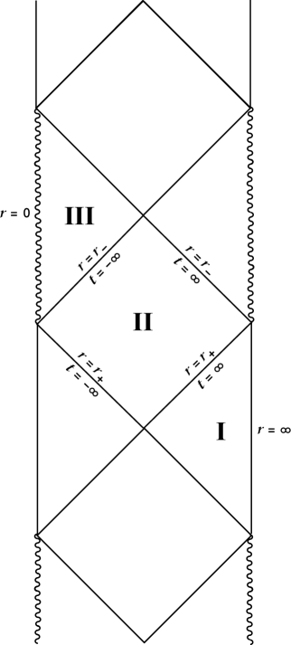
Figure 1: Penrose diagram for maximally extended AdS Reissner-Nordström black hole.

The brane is modelled in the usual thin-brane approximation. That is, its worldvolume is a hypersurface, $\cal B$, which divides the bulk spacetime, $\cal M$, into two regions. At this hypersurface, the bulk metric is continuous but not differentiable. Using the standard Israel junction conditions [14] (see also [15]), the discontinuity in the extrinsic curvature is interpreted as a $\delta$-function source of stress-energy due to the brane. Then, defining the discontinuity in the extrinsic curvature across $\cal B$ as ${{\cal K}}_{ab}\equiv K^{+}_{ab}-K^{-}_{ab}$, the surface stress-tensor is given by

$$S_{ab}={1\over 8\pi G_{5}}\left({\cal K}_{ab}-\gamma_{ab}\,{\cal K}^{c}{}_{c}\right)\ .$$ (2.4)

In the case of an empty brane with only tension (i.e., a brane on which no internal degrees of freedom are excited), one has $S_{ab}=-T\gamma_{ab}$.

The construction of the braneworld cosmology [7] then proceeds by taking two copies of the AdS black hole geometry, identifying a four-dimensional hypersurface $r=a(\tau)$, $t=b(\tau)$ in each, cutting out the spacteime regions beyond these hypersurfaces and ‘gluing’ the two remaining spacetimes along these surfaces. While asymmetric constructions are possible (see e.g., [12]), we will focus on the case where the two bulk spacetime geometries are characterized by the same physical parameters ($\mu,q,L$). With this choice, the calculation of the surface stress-tensor simplifies, since ${\cal K}_{ab}=2K^{+}_{ab}$. Note, however, that the gauge fields are chosen with opposite signs on either side of the brane. Then the flux lines of the bulk gauge field extend continuously over the brane, starting from a positively-charged black hole on one side and ending on the negatively-charged one on the other. In this case, the brane carries no additional charges. We will return to consider a charged brane in the discussion section. Since the black hole geometry includes two separate, asymptotically AdS regions, an economical approach to this construction would be to glue together two mirror surfaces in each of the asymptotic regions.

Of course, the hypersurface described above must be determined to consistently solve the Einstein equations (or alternatively, the Israel junction conditions (2.4)) for a physically reasonable surface stress-tensor. Here we follow the analysis of ref. [7]. Identifying the time coordinate on the brane as the proper time, $\tau$, fixes

$$V(a)\,\dot{b}^{2}={\dot{a}^{2}\over V(a)}+1\ .$$ (2.5)

The induced metric then takes a standard FRW form:

$$ds^{2}=\gamma_{ab}\,dx^{a}dx^{b}=-d\tau^{2}+a(\tau)^{2}d\Sigma_{k}^{2}\ .$$ (2.6)

Again, the brane worldvolume in the bulk spacetime (2.2) is given by $r=a(\tau)$ and $t=b(\tau)$ and so the Israel junction conditions (2.4) imply

$$\frac{\left(V(a)+\dot{a}^{2}\right)^{1/2}}{a}=\frac{1}{\lambda}+\frac{4\pi G_{5}}{3}\rho\ ,$$ (2.7)

where the ‘dot’ denotes $\partial_{\tau}$, and we have included a homogenous energy density $\rho$ for brane matter. Stress-energy conservation would imply that the latter satisfies $\dot{\rho}+3\frac{\dot{a}}{a}\,(\rho+p)=0$, where $p$ is the pressure due to brane matter.

A conventional cosmological or FRW constraint equation for the evolution of the brane is produced by squaring eq. (2.7):

$$\left(\frac{\dot{a}}{a}\right)^{2}+\frac{k}{a^{2}}={1\over\ell^{2}}+\frac{\mu}{a^{4}}-\frac{q^{2}}{3a^{6}}+\left(\frac{1}{T\lambda}\right)^{2}\left(2T\rho+\rho^{2}\right)\ .$$ (2.8)

Here, we have defined a ‘vacuum’ curvature scale on the brane as

$$\frac{1}{\ell^{2}}\equiv\frac{1}{\lambda^{2}}-\frac{1}{L^{2}}\ .$$ (2.9)

Implicitly, $\ell^{2}$ is assumed to be positive here, which leads to the cosmological evolution being asymptotically de Sitter. However, this assumption is inconsequential for analysis of the cosmological bounce which follows. We can also write out the effective cosmological and Newton constants in the four-dimensional braneworld as

$$\Lambda_{4}\equiv{3\over 8\pi G_{4}}{1\over\ell^{2}}=\frac{T}{2}\left(1-\left(\frac{\lambda}{L}\right)^{2}\right)\ ,\qquad\qquad G_{4}\equiv\frac{G_{5}}{\lambda}\ ,$$ (2.10)

where the latter comes from matching the term in eq. (2.8) linear in $\rho$ to the conventional FRW equation in four dimensions: $\left(\frac{\dot{a}}{a}\right)^{2}+\frac{k}{a^{2}}=\frac{8\pi G_{4}}{3}\rho$. Of course, the FRW constraint in this braneworld context also comes with an unconventional term quadratic in $\rho$ [4].

The bulk geometry introduces various sources important in the cosmological evolution of the brane. The mass term, $\mu/a^{4}$, behaves like a conventional contribution coming from massless radiation. The charge term, $-q^{2}/a^{6}$, introduces a more exotic contribution with a negative energy density. This is another example of the often-noted result that the bulk contributions to the effective stress-energy on the brane [16] may be negative — see, e.g., [9].

Many exact and numerical solutions for the Friedmann equation (2.8) can be obtained in various situations, e.g., [10, 11]. However, one gains a qualitative intuition for the solutions in general by rewriting eq. (2.8) in the following form:

$$0=\dot{a}^{2}+U(a)\ ,$$ (2.11)

where

$$U(a) = V(a)-\frac{a^{2}}{\lambda^{2}}$$

$$= k-{\mu\over a^{2}}+{q^{2}\over 3a^{4}}-{a^{2}\over\ell^{2}}$$

and for simplicity we have assumed an empty brane, i.e., $\rho=0$. In this form, we recognize the evolution equation as the Hamiltonian constraint for a classical particle with zero energy, moving in an effective potential $U(a)$. In this case, the transition regions where the braneworld cosmology ‘bounces’ are identified with the turning points of the effective potential. We have also expressed the latter in terms of the metric function $V(a)$ in eq. (2) because we will want to discuss the position of the turning points relative to the position of the ‘horizons’, i.e., $r_{\pm}$. Recall that we assume the bulk solution corresponds to a black hole with a nondegenerate event horizon. That is, we will assume that there are two distinct solutions, $r_{\pm}$, to $V(r)=0$. Then, there are two physically distinct possibilities for a bounce.

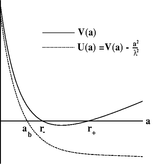
Figure 2: Effective potential, $U(a)$, appearing in eq. (2.11) for the evolution of the scale factor, $a(\tau)$. The turning point, $a_{b}$, occurs inside the Cauchy horizon $r_{-}$.

The first only occurs with $k=+1$, i.e., with a spherical brane world, and positive $\ell^{2}$ (or equivalently $\Lambda_{4}>0$). In this case, at large $a$, the effective potential becomes large and negative. The next most important contribution at large $a$ is the constant term $k$ and hence if $k=+1$, the potential may have a zero at large $a$. This bounce is typical of those one might find in a de Sitter-like spacetime, e.g., [17]. It is driven by the spatial curvature and occurs as long as the effective energy density from the bulk black hole contributions or braneworld degrees of freedom is not too large. The turning point occurs at some large $a_{dS}$ and in particular, it is not difficult to show that $a_{dS}>r_{+}$. That is, the brane bounces before reaching the black hole. In fact the presence of the black hole with or without charge is really irrelevant to this kind of bounce. For example, setting $\mu=0=q$ in eq. (2) produces a de Sitter cosmology on the empty brane.

The second type of bounce is generic for a wide range of parameters. It occurs at small $a$ where the positive $q^{2}/a^{4}$ term dominates the potential (2), i.e., where the exotic negative energy dominates the Friedmann constraint (2.8). As is clear from the first line of eq. (2), $U(a)<V(a)$ and therefore the turning point occurs at $a_{b}$, inside the position of the Cauchy horizon, i.e., $a_{b}<r_{-}$, as illustrated in Figure 2. The latter result will be essential in the following discussion.

The Penrose diagram for the bouncing braneworld cosmologies is shown in Figure 3. In the ‘cut and paste’ procedure outlined above, the singularity on the right side of the first black hole is cut out, but the singularity on the left remains. Hence, the remaining portion of the $r=r_{-}$ surface is still a Cauchy horizon.

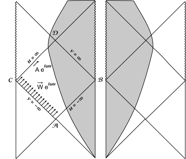
Figure 3: Penrose diagram for a bouncing braneworld model with ingoing modes at the event and Cauchy horizons. The grey areas are those regions of spacetime that are cut out in the construction, with identification performed along the boundary.

Note that in Figure 3, the brane trajectory enters the region between the horizons across the segment $\mathcal{AB}$ and exits across the opposite segment $\mathcal{CD}$. One can verify that this occurs in all cases using eqs. (2.7) and (2.5). From the latter, we find that

$$\dot{t}=\pm\frac{a}{V(a)}\left(\frac{1}{\lambda}+\frac{4\pi G_{5}}{3}\rho\right)\ .$$ (2.13)

If the brane tension and the energy density, $\rho$, are both assumed to be always positive, then the last factor is always positive. Furthermore, for $r_{-}<a<r_{+}$, $V(a)<0$. Hence, the right hand side above is non-zero and has a definite sign for the entire range $r_{-}<a<r_{+}$. Therefore $\dot{t}$ cannot change sign along the brane trajectory within the black hole interior. It then follows that if a trajectory starts at a point on $\mathcal{AB}$ with $(t,r)=(\infty,r_{+})$, then it must run across the black hole interior to a point on $\mathcal{CD}$ with $(t,r)=(-\infty,r_{-})$ — see Figures 1 and 3.

3 Instability Analysis

In the previous section, we reviewed the construction of a broad family of bouncing braneworld cosmologies [6]. A key result was that the turning point for the brane’s trajectory in the bulk geometry was inside the Cauchy horizon of the charged AdS black hole. However, previous studies in classical general relativity found that the Cauchy horizon is unstable when generic perturbations are introduced for charged black holes in asymptotically flat [18], or de Sitter [19, 20] spaces. Below, we will show that the same instability arises in the asymptotically AdS case as well. This is problematic for the bouncing braneworld cosmologies, as generically the contracting brane will reach a curvature singularity before it begins re-expanding.

In the following, we demonstrate the instability of the Cauchy horizon to linearized perturbations in the bulk. Our approach will be two-fold. We begin by examining linearized fluctuations of a massive Klein-Gordon field propagating in the background. Secondly, we consider gravitational and electromagnetic perturbations. In both cases, it is found that an observer crossing the Cauchy horizon would measure an infinite flux from these modes. The expectation is then that the full nonlinear evolution, including the back-reaction on the background metric, will produce a curvature singularity.

Many of the expressions appearing in the linearized analysis involve the surface gravities of the two horizons in the background. The surface gravities are given, as usual, by

$$\kappa_{\pm}=\frac{1}{2}\left|\frac{dV}{dr}\right|_{r=r_{\pm}}\ .$$ (3.14)

An important observation in the following is that $\kappa_{+}/\kappa_{-}<1$, which follows from $r_{-}<r_{+}$. Now it will be convenient to define the event and Cauchy horizons implicitly by re-expressing the metric function (2.3) as

$$V(r)=\frac{(r^{2}-r_{+}^{2})(r^{2}-r_{-}^{2})(r^{2}+r_{0}^{2})}{L^{2}r^{4}}\ .$$ (3.15)

This expression also defines $r_{0}$ as determining the complex roots of $V(r)$. Further, the analysis is facilitated by introducing some new coordinates to describe the background geometry (2.2). In particular, we define the radial tortoise coordinate

$$r_{*}\equiv\frac{1}{2\kappa_{+}}\log\frac{|r-r_{+}|}{r+r_{+}}-\frac{1}{2\kappa_{-}}\log\frac{|r-r_{-}|}{r+r_{-}}+\frac{r_{0}^{3}L^{2}}{(r_{0}^{2}+r_{-}^{2})(r_{0}^{2}+r_{+}^{2})}\tanh^{-1}\frac{r}{r_{0}}\ ,$$ (3.16)

which is chosen to satisfy $dr_{*}=dr/V(r)$. The focus of the following analysis will be the behavior of linearized perturbations in the range $r_{-}<r<r_{+}$ (i.e., region II in Figure 1). In this region, we have $r_{*}\rightarrow\pm\infty$ as $r\rightarrow r_{\mp}$. Finally, it will be useful to work with null coordinates,

$$u=r_{*}-t\ ,\qquad v=r_{*}+t\ ,$$ (3.17)

with which the line element becomes $ds^{2}=V(r)du\,dv+r^{2}d\Sigma^{2}_{k}$.

The massive Klein-Gordon equation in the charged black hole background (2.2) may be expanded as

$$-\frac{1}{V(r)}\partial_{t}^{2}\Phi+V(r)\partial_{r}^{2}\Phi+\frac{1}{\sqrt{-g}}\partial_{r}\left(\sqrt{-g}~{}V(r)\right)\partial_{r}\Phi+\frac{1}{r^{2}}\nabla_{k}^{2}\Phi-M^{2}\Phi=0\ ,$$ (3.18)

where we write $\nabla^{2}_{k}$ for the Laplacian on the three-dimensional space $\Sigma_{k}$ appearing in the line element (2.2). The eigenvalue problems for $\partial_{t}^{2}$ and $\nabla_{k}^{2}$ each have known solutions with eigenvalues, say, $-\omega^{2}$ and $-n^{2}_{k}$. Hence by separation of variables, the Klein-Gordon equation is reduced to a single ordinary differential equation for $\Phi(r)$,

$$-\partial_{r_{*}}^{2}\tilde{\Phi}+V(r)\left(\frac{n_{k}^{2}}{r^{2}}+M^{2}+\frac{3V^{\prime}}{2r}+\frac{3V}{4r^{2}}\right)\tilde{\Phi}=\omega^{2}\,\tilde{\Phi}\ ,$$ (3.19)

where we have introduced the tortoise coordinate (3.16) and rescaled $\tilde{\Phi}=r^{3/2}\Phi$.

As we approach the Cauchy horizon, the second term on the left hand side of eq. (3.19) vanishes, leading to oscillatory solutions $\exp(\pm i\omega r_{*})$. Now, the flux seen by an observer freely falling across the horizon, with five-velocity $U^{\mu}$, is proportional to the square of the scalar ${\cal F}=U^{\mu}\partial_{\mu}\Phi$. $\cal F$ then includes a contribution proportional to $e^{\kappa_{-}u}\partial_{u}\tilde{\Phi}$ near the Cauchy horizon. Since the solutions of eq. (3.19) are oscillatory as $r\rightarrow r_{-}$, we have that this term, and hence ${\cal F}$, diverges. Similar divergences appear in the observed energy density for these linearized perturbations, and so the expectation is that when back-reaction is included, the metric will develop a curvature singularity.

Next we proceed to a more rigorous analysis of metric and Maxwell field perturbations, following the method of Chandrasekhar and Hartle [18]. We are simply establishing the existence of unstable modes and so, for simplicity, we fix $k=0$ and consider an “axial” perturbation of one of the flat space coordinates. However, the extension of this analysis to general perturbations and backgrounds is straightforward.

The unperturbed bulk metric (2.2) is

$$ds^{2}=-V(r)\,dt^{2}+\frac{dr^{2}}{V(r)}+\frac{r^{2}}{L^{2}}(dx^{2}+dy^{2}+dz^{2})\ ,$$ (3.20)

where $V(r)$ is as given in eq. (2.3) with $k=0$. We now focus on a class of perturbations where this metric is modified by replacing

$$dz\rightarrow dz+q_{t}(t,r)dt+q_{r}(t,r)dr\ .$$ (3.21)

Similarly for the Maxwell field, we introduce perturbations: $\delta{\mathbf{F}}=(f_{tz}(t,r){\mathbf{d}}t+f_{rz}(t,r){\mathbf{d}}r)\wedge{\mathbf{d}}z$. The linearization of the bulk Einstein and Maxwell equations about the background solution may be reduced to a single Schrödinger-like equation:

$$-\partial_{r_{*}}^{2}F+\frac{V}{r}\left(\frac{4q^{2}}{r^{5}}-\frac{V}{4r}+\frac{V^{\prime}}{2}\right)F=\omega^{2}\,F\ .$$ (3.22)

In this equation, we have defined $F\equiv r^{1/2}f_{tz}$ and assumed an $e^{-i\omega t}$ dependence for all fields. To apply the standard results of scattering theory below, it is important to note that the effective potential (i.e., the pre-factor in the second term on the left hand side) is bounded, negative and integrable throughout the black hole interior. Further, we note that the effective potential vanishes as $\exp\left({\pm\kappa_{\pm}r_{*}}\right)$ for $r_{*}\rightarrow\mp\infty$. The other components of the perturbation are related to $F$ by

$$f_{rz} = \frac{i}{\omega}\partial_{r}(F/r^{1/2})\ ,$$

$$Q_{tr} = -4i\frac{q\,L^{2}}{\omega\,r^{11/2}}F\ ,$$ (3.23)

where $Q_{tr}=\partial_{t}q_{r}-\partial_{r}q_{t}$. Note that the linearized equations only fix the metric perturbations, $q_{r}$ and $q_{t}$, up to infinitesimal coordinate transformations of $z$, but $Q_{tr}$ provides a gauge invariant combination which is completely determined.

We introduce a basis of solutions to eq. (3.22) normalized so that near the event horizon, i.e., $r_{*}\rightarrow-\infty$,

$$\stackrel{{\scriptstyle\rightarrow}}{{F}}(\omega,r_{*}) \rightarrow e^{i\omega r_{*}}\ ,$$

$$\stackrel{{\scriptstyle\leftarrow}}{{F}}(\omega,r_{*}) \rightarrow e^{-i\omega r_{*}}\ ,$$ (3.24)

representing, respectively, ingoing and outgoing modes. The full solution to (3.22) may then be written as

$$F(t,r_{*})=\int^{\infty}_{-\infty}\frac{d\omega}{2\pi}\left[\stackrel{{\scriptstyle\leftarrow}}{{W}}(\omega)\stackrel{{\scriptstyle\leftarrow}}{{F}}(\omega,r_{*})+\stackrel{{\scriptstyle\rightarrow}}{{W}}(\omega)\stackrel{{\scriptstyle\rightarrow}}{{F}}(\omega,r_{*})\right]e^{-i\omega t}\ .$$ (3.25)

At present, we are only interested in the ingoing modes, whose profile is determined by $\stackrel{{\scriptstyle\rightarrow}}{{W}}(\omega)$. The outgoing modes may be similarly dealt with, but extra analysis would be required to show they lead to a divergent flux. We will return to this point near the end of the section.

We are free to choose any reasonable initial profile for the ingoing modes. However, one restriction which we impose on the initial frequency distribution $\stackrel{{\scriptstyle\rightarrow}}{{W}}(\omega)$ of ingoing modes is that an observer falling across the event horizon at $\mathcal{AB}$ measures a finite flux. The flux for such an observer contains a term $\mathcal{F}\sim e^{-\kappa_{+}u}\partial_{u}F$. Hence considering eq. (3.25), we require that $\stackrel{{\scriptstyle\rightarrow}}{{W}}(\omega)$ have at least one pole with $\mathfrak{Im}(\omega)\leq-\kappa_{+}$.

The initially-ingoing modes are scattered by the potential in region II, leading to both ingoing and outgoing modes at the Cauchy horizon. Scattering theory will be used to relate the functions introduced in (3.24) to a second set normalized so that, as $r_{*}\rightarrow\infty$,

$$\stackrel{{\scriptstyle\rightarrow}}{{F}}(\omega,r_{*})e^{-i\omega t} \rightarrow \left(A(\omega)e^{i\omega r_{*}}+B(\omega)e^{-i\omega r_{*}}\right)e^{-i\omega t}\$$ (3.26)

$$\quad=A(\omega)e^{i\omega u}+B(\omega)e^{-i\omega v}\ .$$

Clearly, the dominant contribution to the flux at the Cauchy horizon results from

$${\mathcal{F}}\sim e^{\kappa_{-}u}\int^{\infty}_{-\infty}d\omega\ \omega\stackrel{{\scriptstyle\rightarrow}}{{W}}(\omega)A(\omega)e^{i\omega u}\ .$$ (3.27)

In terms of the Schrödinger equation describing the perturbations, it is the modes that are “transmitted” across the potential that constitute this potentially-divergent flux. These modes skim along just outside the Cauchy horizon heading towards the brane.

The integral in (3.27) may be computed by closing the contour in the upper-half-plane. Using arguments from [18], with virtually no modification, we find that $\omega A(\omega)$ is analytic in the infinite strip between $\pm i\kappa_{+}$. For simplicity, we’ll further assume that $\stackrel{{\scriptstyle\rightarrow}}{{W}}(\omega)$ is analytic in the strip $[0,i\kappa_{+}]$ and that it is non-zero for $\omega=i\kappa_{+}$. With these assumptions, the leading term in (3.27) is from the residue of the pole at $\omega=i\kappa_{+}$:

$${\mathcal{F}}\sim e^{(\kappa_{-}-\kappa_{+})u}\left\{i\kappa_{+}\stackrel{{\scriptstyle\rightarrow}}{{W}}(i\kappa_{+})2\pi i~{}\mbox{Res}\left(A(i\kappa_{+})\right)\right\}\ .$$ (3.28)

Since $\kappa_{-}>\kappa_{+}$, this flux always diverges as $u\rightarrow\infty$. Relaxing our assumptions on the analyticity of $\stackrel{{\scriptstyle\rightarrow}}{{W}}(\omega)$ in the upper half plane could lead to additional divergent contributions to the flux, but we will not consider those here.

Note that the brane and boundary conditions at the brane played no role in the scattering analysis above. While the brane will affect the complete scattering of modes inside the event horizon, the basic source of the instability is the same piling up of infalling modes on the Cauchy horizon found in previous examples [18, 19]. Hence we disregard the details of the scattering of modes at the brane, just as the original discussion of the instability for the Reissner-Nordström black hole [18] ignored the presence of a collapsing star forming the black hole.

However, for completeness, let us briefly discuss the boundary conditions which must be imposed on the perturbations at the brane. First, the metric perturbations must be matched across the brane surface so that no additional contributions are induced in the surface stress-energy (2.4). In particular, the axial perturbation (3.21) considered above induces a new $K_{\tau z}$ component in the extrinsic curvature, and this component must be continuous across the brane. Similarly, continuity is imposed on the Maxwell field strength. More precisely, to ensure that no electric charges or currents are implicitly induced on the brane, we require that all components $n^{\mu}F_{\mu\nu}t^{\nu}$ are continuous, where $n^{\mu}$ and $t^{\nu}$ are the unit normal and any tangent vector to the brane. Finally, since we are working with perturbations to the field strength directly, and not the gauge potential, we must demand continuity of the tangential components, $t_{1}^{\mu}F_{\mu\nu}t_{2}^{\nu}$, to ensure there are no magnetic charges or currents induced, i.e., $\mathbf{dF}=0$.

We close this section with a discussion of the initially-outgoing modes defined by the distribution $\stackrel{{\scriptstyle\leftarrow}}{{W}}(\omega)$ in eq. (3.25). In Figure 3, we will primarily consider modes entering the interior region on the left through the lower portion of $\mathcal{AB}$. In this case, to contribute to the instability at the Cauchy horizon $\mathcal{CD}$, these modes must be reflected by the curvature (i.e., by the effective potential in eq. (3.22) to become ingoing. This scattering leads to a different analytic structure in eq. (3.26) for $A(\omega)$, describing the $u$-dependent modes at the Cauchy horizon. In the “un-cut” spacetime with no brane in place, this structure is identical to that obtained for the contribution of the initially-ingoing modes to $B(\omega)$. Of course, inserting the brane in the black hole interior produces a more complicated scattering problem, the details of which would depend on the precise brane trajectory. For example, the outgoing flux would receive additional contributions from perturbations transmitted across the brane from the right hand side of Figure 3, as well as from initially-ingoing modes which are back-scattered by the brane. We did not attempt a detailed study of these contributions.

Now , following the standard analysis with no brane in place, we find that the contribution to $\omega A(\omega)$ from the outgoing modes is analytic in the semi-infinite strip $(-i\kappa_{+},i\kappa_{-})$. If we assume that $\stackrel{{\scriptstyle\leftarrow}}{{W}}(\omega)$ is analytic in the strip $(0,i\kappa_{-})$, then we would find, upon closing the contour in the upper-half-plane, that the contribution to the flux is finite. However, it is consistent with the requirement that an observer crossing $\mathcal{AC}$ measure a finite flux, to allow $\stackrel{{\scriptstyle\leftarrow}}{{W}}(\omega)$ to have poles in the range $\kappa_{+}\leq\mathfrak{Im}(\omega)<\kappa_{-}$. With such a choice, there will be divergent contributions to the flux, provided that the residue of $A$ is non-zero at these poles. This effect differs from that discussed above in that the leading contribution to the flux comes from a pole in the initial frequency distribution rather than the scattering coefficient $A(\omega)$. A similar discussion played an important role in demonstrating the instability of the Cauchy horizon of de Sitter-Reissner-Nordström black holes over the entire range of physical parameters [20].

4 Discussion

One of the most interesting features of the braneworld cosmologies presented in ref. [6] is that, while they seem to evade any cosmological singularities, their evolution is still determined by a simple effective action, albeit in five dimensions. However, our present analysis indicates that instabilities arise in the five-dimensional spacetime, and that the brane will generically encounter a curvature singularity before bouncing. The two essential observations leading to this result were: i) the turning point for the brane cosmology occurs inside the Cauchy horizon of the maximally-extended geometry of the charged AdS black hole and ii) a standard analysis within classical general relativity shows that the Cauchy horizon is unstable against even small excitations of the bulk fields. Note that from these results we cannot conclude that the brane does not bounce, but rather due to the appearance of curvature singularities, the evolution can not be reliably studied with the original low energy action (2.1).

Of course, one may ultimately have reached this conclusion since the full bulk spacetime still includes a curvature singularity at $r=0$ — see Figure 3. However, while the latter remains distant from the brane, those at the Cauchy horizon are of more immediate concern as they intersect the brane’s trajectory.

In the discussion of metric and gauge field perturbations in section 3, we fixed $k=0$ and limited ourselves to modes that depended only on $t$ and $r$ to simplify the discussion. One may be concerned by the fact that these modes have infinite extent in the three-dimensional flat space and so we present a brief discussion of the full analysis. Generalizing our results to the most general perturbation is straightforward but tedious. For an arbitrary linearized perturbation, the separation of variables would naturally lead to considering Fourier components in the ($x,y,z$) directions with a factor $\exp\left(i\vec{n}\cdot\vec{x}\right)$. Since we require a superposition of these modes for many different $\vec{n}$ to localize the perturbation, we cannot simply rotate in the flat space to remove the dependence on one of the spatial coordinates. Thus the general analysis necessarily involves an ansatz for the perturbations dependent on all five coordinates, which, of course, requires extending the perturbations to additional components of both the metric and gauge field. Appropriate linear combinations of these perturbations would decouple, giving a set of Schrödinger-like equations, similar to that found above. While the potentials in each of these equations is different, there are typically simple relationships between them implying relations between the solutions — for further discussion of these relations, see [18]. Then it is sufficient to solve only one of the equations, and the analysis, and the results, are essentially the same as presented above

Of course, our preliminary analysis with massive Klein-Gordon modes included all of the spatial modes, and further applied for all of the possible values of $k$, specifying the spatial curvature on the brane. In all cases, there was an infinite flux of these modes at the Cauchy horizon. While further analysis of the full scattering and boundary conditions would be required to make this consideration of fluxes rigorous, the end result would be the same. Hence we are confident that the results for the metric and gauge field perturbations with $k=0$ also carry over for $k=\pm 1$.

Recall that, as discussed in section 2, an apparently economical approach to constructing these bouncing cosmologies would be to cut and paste along two mirror surfaces in each of the separate asymptotically AdS regions of the black hole geometry. In such a periodic construction the nature of the singular behavior would be slightly different. As discussed around eq. (2.13), the brane trajectory is unidirectional in the coordinate time, $t$. Hence in Figure 3, if a brane enters the event horizon to the right of the bifurcation surface ${\mathcal{A}}$, then it must exit through the Cauchy horizon to the left of ${\mathcal{D}}$. However, the same result requires that a brane trajectory entering to the left of ${\mathcal{A}}$ exits to the right of ${\mathcal{D}}$. Therefore in the periodic construction above, the two mirror trajectories must cross at some point in the region $r_{-}<r<r_{+}$, as illustrated in Figure 4. Hence, the evolution is singular in that the fifth dimension collapses to zero size in a finite proper time. One redeeming feature of this collapse is that the curvature remains finite, and hence one might imagine that there is a simple continuation of the evolution in which this ‘big crunch’ is matched onto a ‘big bang’ geometry. Similar collapsing geometries have been a subject of great interest in the string theory community recently — see, e.g., [21, 22]. Resolving precisely how the spacetime evolves beyond such a ‘big crunch’ is an extremely difficult question and as yet string theory seems to have produced no clear answer. In particular, it seems that these geometries are also subject to gravitational instabilities [23] not dissimilar to those found here. In the present context, the situation is further complicated as the precise matching procedure for the background geometry is obscure. Naively, one might be tempted to continue beyond the collapse point $\mathcal{E}$ with the doubly shaded region in Figure 4. However, a closer examination shows that the brane would have a negative tension in this geometry. The other natural alternative is to match the crunch at $\mathcal{E}$ to the big bang emerging from $\mathcal{F}$, but the gap in the embedding geometry would seem to complicate any attempts to make this continuation precise. In any event, it is clear that once again these knotty questions can not be resolved using the low energy action (2.1) alone but, rather, one would have to embed this scenario in some larger framework, e.g., string theory.

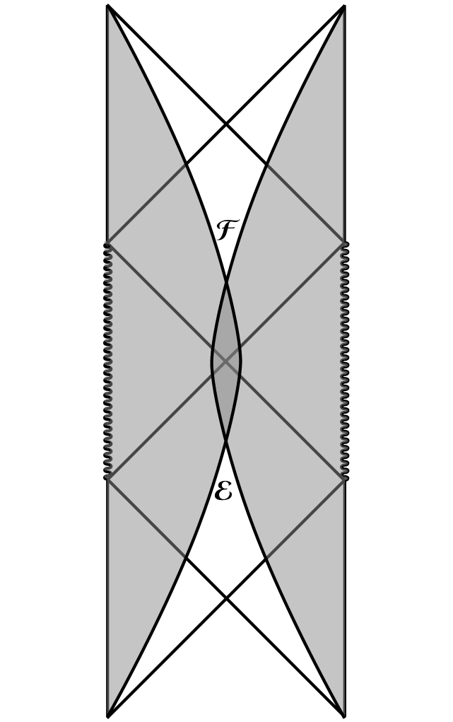
Figure 4: Penrose diagram for periodic construction of the braneworld cosmology

Much of our discussion has focussed on the bouncing cosmologies for an empty four-dimensional brane, but the analysis and the results are easily extended to other cases. One simple generalization would be for higher dimensional cosmologies following, e.g., [11]. The instability found here would also appear in the assymetric constructions discussed in ref. [12].

A more interesting generalization to consider is adding matter excitations on the brane. As long as the energy density is positive, such matter contributions will not affect the result that the brane crosses the Cauchy horizon. At first sight, it would also seem that reasonable brane matter cannot prevent the bounce. The negative energy contribution arising from the bulk charge is proportional to $1/a^{6}$. For a perfect fluid (in four dimensions), this would require the stiffest equation of state consistent with causality [24], i.e., $p=\rho$. For example, a coherently rolling massless scalar field would yield $\rho\propto 1/a^{6}$. Hence it would seem that the term $-q^{2}/a^{6}$ would dominate the $\rho$ contribution coming from brane matter and a bounce would be inevitable. However, ref. [12] recently pointed out the $\rho^{2}$ contribution in the FRW constraint (2.8) can prevent a bounce. In fact, with any equation of state $p=w\rho$ with $w\geq 0$, this contribution can dominate the bulk charge contribution. Hence with a sufficiently large initial energy density on the brane, a big crunch results on the brane. This crunch corresponds to the brane trajectory falling into the bulk singularity at $r=0$. It then follows that the brane must cross the Cauchy horizon in this case as well, and we expect singularities to develop there with generic initial data.

More broadly, mirage cosmologies [5] are induced by the motion of a brane in a higher dimensional spacetime. A general warning which the present analysis holds for these models is that Cauchy horizons are quite generally unstable. Hence if a particular solution involves a brane traversing such a surface in the bulk spacetime, one should expect that these cosmologies will encounter singularities for generic initial data.

At this point, we observe that in the literature much of the discussion of these brane cosmologies treats the brane as a fixed point of a $Z_{2}$ orbifold, rather than making a symmetric construction as discussed in section 2. As discussed there, one must flip the sign of the gauge potential in the background solution on either side of the brane in order that the brane is transparent to field lines. In contrast for a $Z_{2}$ orbifold, the field lines end on the brane. As there is no natural coupling of a one-form potential to a three-brane in five dimensions, the model must be extended to include charged matter fields on the brane. One comment is that as the action (2.1) does not explicitly include these degrees of freedom or their coupling to the Maxwell field, we cannot be sure that the analogous construction to that presented in section 2 will yield a consistent solution of all of the degrees of freedom. One might also worry that the simplest solutions would have additional instabilities associated with having a homogeneous charge distribution throughout the brane.

Bouncing cosmologies have long been of interest [25]. Much of their appeal lies in their potential to provide a calculable framework to describe the origins of the universe. Apart from the present discussion, braneworlds and higher dimensions have inspired many attempts to model a bouncing cosmology, including: pre-big bang cosmology [26]; cyclic universes [27] based on a Lorentzian orbifold model [21]; braneworld cosmologies induced by cyclic motion in more than one extra dimensions [28]; universes with higher form fluxes [30, 31], which are related to S-brane solutions [32]; braneworld cosmologies [33] with an extra internal time directions [34]. However, as well as the present model, none of these works has yet provided a compelling scheme which is free of pathologies or obstructions to prediction. We may take solace from the absence of any simple bounce models in that it appears that understanding the early universe and, in particular, the big bang singularity demands that we greatly expand our understanding of quantum gravity and string theory.