M-THEORY COMPACTIFICATIONS,
$G_{2}$-MANIFOLDS AND ANOMALIES

DIPLOMARBEIT

VON

STEFFEN METZGER

LABORATOIRE DE PHYSIQUE THÉORIQUE

PROF. DR. A. BILAL

ÉCOLE NORMALE SUPÉRIEURE

PARIS

und

SEKTION PHYSIK

LEHRSTUHL FÜR MATHEMATISCHE PHYSIK

PROF. DR. J. WESS

LUDWIG-MAXIMILIANS-UNIVERSITÄT MÜNCHEN

Abstract

This diploma thesis has three major objectives. Firstly, we give an elementary introduction to M-theory compactifications, which are obtained from an analysis of its low-energy effective theory, eleven-dimensional supergravity. In particular, we show how the requirement of $\mathcal{N}=1$ supersymmetry in four dimensions leads to compactifications on $G_{2}$-manifolds. We also examine the Freund-Rubin solution as well as the M2- and M5-brane. Secondly, we review the construction of realistic theories in four dimensions from compactifications on $G_{2}$-manifolds. It turns out that this can only be achieved if the manifolds are allowed to carry singularities of various kinds. Thirdly, we are interested in the concept of anomalies in the framework of M-theory. We present some basic material on anomalies and examine three cases where anomalies play a prominent role in M-theory. We review M-theory on $\mathbb{R}^{10}\times S^{1}/\mathbb{Z}_{2}$ where anomalies are a major ingredient leading to the duality between M-theory and the $E_{8}\times E_{8}$ heterotic string. A detailed calculation of the tangent and normal bundle anomaly in the case of the M5-brane is also included. It is known that in this case the normal bundle anomaly can only be cancelled if the topological term of eleven-dimensional supergravity is modified in a suitable way. Finally, we present a new mechanism to cancel anomalies which are present if M-theory is compactified on $G_{2}$-manifolds carrying singularities of codimension seven. In order to establish local anomaly cancellation we once again have to modify the topological term of eleven-dimensional supergravity as well as the Green-Schwarz term.

Für meine Eltern

Chapter 1 Introduction

The fundamental degrees of freedom of M-theory are still unknown. Nevertheless, over the last few years indication has been found that M-theory is a consistent quantum theory that contains all known string theories as a certain limit of its parameter space. Like string theory, M-theory comprises both general relativity and quantum field theory and therefore might well be a major step towards a unified theory of all the forces in nature.
As is well known, M-theory needs to be formulated in eleven dimensions. So in order to make this model realistic we have to ask whether there is a vacuum of the theory that contains only four macroscopic dimensions, with the other seven dimensions compact and small and hence invisible.
Experimental data - for instance the huge difference in energy between the electroweak scale and the Planck scale, also known as the hierarchy problem - tell us that our world can most probably be described by a quantum theory with $\mathcal{N}=1$ supersymmetry [79], [80], [77]. At some other scale - that might even be reached by present day’s accelerators - this supersymmetry has to be broken again, of course, as we do not observe any superpartners of the known particles.
So what we want to study are M-theory vacua with $\mathcal{N}=1$ supersymmetry and four macroscopic space-time dimensions. There are two known ways to obtain such theories from M-theory. The first possibility is to compactify M-theory on a space $\mathbb{R}^{3,1}\times X$, where $X$ is a manifold with boundary $\partial X$, and $\partial X$ is a Calabi-Yau manifold [57], [58]. The basic setup of this approach will be described in chapter 4. The second possibility is to take X to be a manifold with holonomy group $G_{2}$. This approach will be analyzed in detail in chapters 5 to 8.
The low-energy effective action of M-theory is eleven-dimensional supergravity [83]. So if $X$ is large compared to the Planck scale, and smooth, supergravity will give a good approximation for low energies. Thus, in order to study M-theory on a given space $\mathbb{R}^{3,1}\times X$, it will be sufficient for most purposes to consider the compactification of its low-energy limit. These sorts of compactification have been studied for quite some time [40]. They are well understood, as eleven-dimensional supergravity is well-defined at least on the classical level.
Yet, once we have obtained a four-dimensional theory, we certainly want to go further. We want to reproduce the field content of the standard model in its very specific form. In particular, there should be non-Abelian gauge groups and charged chiral fermions. It was shown in [82], however, that this field content cannot be achieved by compactifying on smooth manifolds. Indeed, the compactification on a smooth $G_{2}$-manifold, which will be performed explicitly in chapter 5, gives only Abelian gauge groups and neutral chiral multiplets. Nevertheless, there is a possibility to derive interesting theories from compactifications. This is achieved by using an idea that has been popular in string theory over the last years. Usually physicists only work with smooth manifolds, but it turns out that this approach is too restrictive and that it is useful to admit spaces carrying singularities. When these singularities are present, new effects occur, and we will show that it is possible to obtain both charged chiral fermions and non-Abelian gauge groups from compactifications on singular spaces. As will be explained in chapters 7 and 8, conical singularities in the compact seven-manifold $X$ lead to chiral fermions, whereas $ADE$ singularities, singularities of codimension four, in $X$ yield non-Abelian gauge groups. It is clear that the concept of a manifold is no longer valid for these singular spaces, which complicates the mathematical description. Often one needs to leave the familiar grounds of differential geometry and resort to the methods of algebraic geometry so as to give a mathematically precise analysis of these spaces.
It turns out that one of the most important tools which can be used in M-theory calculations are anomalies. It is well-known that anomalies of local gauge symmetries have to vanish in order to render the theory unitary and hence well-defined. Thus, we get rather strong conditions on the theories under consideration. This is particularly useful because anomalies are an infrared effect, implying that an anomaly of the low-energy effective theory destroys the consistency of the full M-theory. That way we can infer information about the full quantum theory.
The main objective of this work is to understand M-theory compactifications on singular spaces carrying holonomy $G_{2}$. For that purpose we provide some mathematical background material in chapter 2, where the mathematics of $G_{2}$-manifolds is described in detail and examples of both compact and non-compact $G_{2}$-manifolds are given.
Chapter 3 lists some background material from physics, namely the basics of eleven-dimensional supergravity, anomaly theory and Kaluza-Klein theory.
In chapter 4 we perform our first M-theory calculation by explaining the duality between M-theory and $E_{8}\times E_{8}$ heterotic string theory. This chapter emphasizes the importance of anomalies in M-theory and explains some ideas and techniques which are also useful in the different context of compactifications on $G_{2}$-manifolds.
The general tack to find M-theory vacua is described in chapter 5, where we give several solutions of the equations of motion of eleven-dimensional supergravity. In particular, we show that the direct product of Minkowski space and a $G_{2}$-manifold is a possible vacuum with $\mathcal{N}=1$ supersymmetry. We also describe the $M2$- and $M5$-brane solutions and comment on their basic properties. Finally, we perform the explicit compactification of eleven-dimensional supergravity on a smooth compact manifold with holonomy $G_{2}$.
Chapter 6 gives the details of anomaly cancellation in M-theory in the presence of $M$-branes. Again the techniques of this chapter are important for understanding the case of $G_{2}$-manifolds.
In chapter 7 we review how realistic theories can arise from compactifications on singular spaces. In order to do so, we explain the duality of M-theory on $K3$ and the heterotic string on the torus $T^{3}$. We show that at certain points in moduli space the $K3$ surface develops $ADE$ singularities which lead to enhanced gauge symmetries. These singularities can be embedded into a $G_{2}$-manifold leading to non-Abelian gauge groups in four dimensions. Chiral fermions arise from compactifications on spaces containing conical singularities.
To confirm these results, we perform an anomaly analysis of M-theory on these singular spaces in chapter 8. We find that the theory is anomaly-free if chiral fermions and non-Abelian gauge groups are present. Details of the methods and ideas used in this chapter can be found in [22] and [23].
We have added a number of appendices, mainly to fix our notation. After a short presentation of the general notation we give some details on Clifford algebras and spinors in appendix B. Appendix C provides the basic formulae for general gauge theories and in appendix D we derive some relations in the vielbein formalism of gravity. Some basic results on index theorems are given in appendix E, while the $ADE$ subgroups of $SU(2)$ are listed in appendix F.

Chapter 2 Preliminary Mathematics

In this chapter we collect the results from mathematics that are necessary to understand the physical picture of M-theory compactified on $G_{2}$-manifolds. Our definitions and notations follow closely those of [63], which is the general reference for this chapter.

2.1 Some Facts from Algebraic Geometry

In this section we present some basic definitions from algebraic geometry. The aim is to understand the concept of the blow-up of a singularity.
First of all, however, we want to give the definition of an orbifold, which we will need many times.

Definition 2.1
A real orbifold is a topological space which admits an open covering $\{U_{i}\}$, such that each patch $U_{i}$ is isomorphic to $\mathbb{R}^{n}/G_{i}$, where the $G_{i}$ are finite subgroups of $GL(n,\mathbb{R})$.
A complex orbifold is a topological space with coordinate patches biholomorphic to $\mathbb{C}^{n}/G_{i}$ and holomorphic transition functions. Here the $G_{i}$ are finite subgroups of $GL(n,\mathbb{C})$.

Definition 2.2
An algebraic set in $\mathbb{CP}^{n}$ is the set of common zeros of a finite number of homogeneous polynomials $h:\mathbb{CP}^{n}\rightarrow\mathbb{C}$. An algebraic set in $\mathbb{CP}^{n}$ is said to be irreducible if it is not the union of two algebraic sets in $\mathbb{CP}^{n}$. An irreducible algebraic set is called a projective algebraic variety. An algebraic variety or simply variety is an open subset of a projective algebraic variety.

Definition 2.3
Let $X$ be a variety in $\mathbb{CP}^{n}$ and let $x\in X$. $x$ is called a nonsingular point if $X$ is a complex submanifold of $\mathbb{CP}^{n}$ in a neighbourhood of $x$. If $x$ is not nonsingular it is called singular. The variety $X$ is called singular if it contains at least one singular point, otherwise it is nonsingular.

Next we present the definition of a blow-up. This can be given for points or subspaces in manifolds as well as in algebraic varieties. The definitions will not be very precise but should give an idea of the basic mechanism. Details can be found in [53].

Definition 2.4
We start with the blow-up of the origin in a disc $\Delta$ in $\mathbb{C}^{n}$. Let $z:=(z_{1},\ldots,z_{n})$ be Euclidean coordinates in $\Delta$ and $l:=[l_{1},\ldots,l_{n}]$ homogeneous coordinates in $\mathbb{CP}^{n-1}$. Define $\widetilde{\Delta}\subset\Delta\times\mathbb{CP}^{n-1}$ as

$$\widetilde{\Delta}:=\{(z,l):z_{i}l_{j}=z_{j}l_{i},\ \forall i,j\},$$ (2.1)

and a projection $\pi:\widetilde{\Delta}\rightarrow\Delta$ by $\pi(z,l):=z$. For $z\neq 0$ this is an isomorphism and $\pi^{-1}(0)$ is the projective space of lines in $\Delta$. The pair $(\widetilde{\Delta},\pi)$ is called the blow-up of $\Delta$ at 0.

Next we define blow-ups of points of manifolds. Let $M$ be a complex $n$-manifold, $x$ a point in $M$ and let $(U,\phi)$ be a chart on $M$ centered around $x$, s.t. $\phi:U\rightarrow\Delta$. Define $\widetilde{\Delta}$ as before then we have another projection $\pi^{\prime}:\widetilde{\Delta}\rightarrow U$ given by $\pi^{\prime}:=\phi^{-1}\circ\pi$. With $E:=\pi^{{}^{\prime}-1}(x)$ we see that $\pi^{\prime}$ is an isomorphism on $\widetilde{\Delta}\backslash E$. The blow-up of $M$ at $x$ is defined as

$$\widetilde{M}:=M\backslash\{x\}\cup\widetilde{\Delta},$$ (2.2)

obtained by replacing $U\subset M$ by $\widetilde{\Delta}$, together with the natural projection $\pi:\widetilde{M}\rightarrow M$.

Finally, we give the definition of the blow-up of a disc along a coordinate plane. Let $\Delta\subset\mathbb{C}^{n}$ be defined as before and take $V\subset\Delta$, s.t. $V:=\{(z_{1},\ldots,z_{n}):z_{k+1}=\ldots=z_{n}=0\}$. Furthermore we take $[l_{k+1},\ldots,l_{n}]$ to be homogeneous coordinates in $\mathbb{CP}^{n-k-1}$. Define $\widetilde{\Delta}\subset\Delta\times\mathbb{CP}^{n-k-1}$ by

$$\widetilde{\Delta}:=\{(z,l):z_{i}l_{j}=z_{j}l_{i},\ k+1\leq i,j\leq n\}.$$ (2.3)

As before the projection $\pi:\widetilde{\Delta}\rightarrow\Delta$ is an isomorphism away from $V$, while $\pi^{-1}(x)\cong\mathbb{CP}^{n-k-1}$ for $x\in V$. The pair $(\widetilde{\Delta},\pi)$ is called the blow-up of $\Delta$ along $V$. This definition can be extended to the blow-up of a manifold $M$ along a submanifold $N$ in $M$ [53].

Furthermore, it is possible to define the blow-up of an algebraic variety $X$ either at a point or along a subset $Y$ of $X$. The result will again be an algebraic variety. We will not give any details concerning the blow-up of varieties but the example of the blow-up of $\mathbb{C}^{2}/\mathbb{Z}_{2}$ given below should clarify the procedure. For singular varieties the blow-up is particularly useful, as is shown by the following theorem.

Theorem 2.5
Let $X$ be a singular variety. Then there exists a nonsingular variety $\widetilde{X}$, which is the result of a finite sequence of blow-ups of $X$.

The blow-up is defined along a subvariety of $X$. If $Y$ is the set of singularities of $X$ this subvariety is naturally taken to be $Y$. The theorem states that either the blow-up of $X$ along $Y$ is already nonsingular or we can continue this process until we get a nonsingular variety. The physical picture is that the singularities are cut out of the variety and a smooth manifold is glued in instead.

Example: The blow-up of $\mathbb{C}^{2}/\mathbb{Z}_{2}$ at 0
The following illustrative example is taken from [11]. Consider $\sigma:\mathbb{C}^{2}\rightarrow\mathbb{C}^{2}$ with $\sigma(z^{1},z^{2}):=(-z^{1},-z^{2})$. Then $\mathbb{C}^{2}/\langle\sigma\rangle\cong\mathbb{C}^{2}/\mathbb{Z}_{2}$ is a complex orbifold and can be understood as a singular algebraic variety. It can be embedded into $\mathbb{C}^{3}$ as

$$\mathbb{C}^{2}/\mathbb{Z}_{2}\cong S:=\{(z_{0},z_{1},z_{2})\in\mathbb{C}^{3}:z_{0}z_{1}-z_{2}^{2}=0\}.$$ (2.4)

The hypersurface $S$ is singular at the origin of $\mathbb{C}^{3}$ and smooth otherwise. $S$ can be parameterized by $z_{0}=\zeta^{2}$, $z_{1}=\eta^{2}$ and $z_{2}=\zeta\eta$. Then $(\zeta,\eta)$ and $(-\zeta,-\eta)$ denote the same point, hence $S$ describes the orbifold $\mathbb{C}^{2}/\mathbb{Z}_{2}$.
According to the prescription given above we consider the following subspace of $\mathbb{C}^{3}\times\mathbb{CP}^{2}$,

$$\widetilde{\mathbb{C}^{3}}:=\{((z_{0},z_{1},z_{2}),[l_{0},l_{1},l_{2}])\in\mathbb{C}^{3}\times\mathbb{CP}^{2}:z_{i}l_{j}=z_{j}l_{i},\ \forall i,j\}.$$ (2.5)

Fixing a non-zero point in $\mathbb{C}^{3}$ gives a single point in $\mathbb{CP}^{2}$. On the other hand for $(z_{0},z_{1},z_{2})=(0,0,0)$ we get an entire $\mathbb{CP}^{2}$. Defining $\pi:\widetilde{\mathbb{C}^{3}}\rightarrow\mathbb{C}^{3}$ in the natural way we found the blow-up $(\widetilde{\mathbb{C}^{3}},\pi)$ of $\mathbb{C}^{3}$ in 0. What we did so far is to excise the origin in $\mathbb{C}^{3}$ and glue in a copy of $\mathbb{CP}^{2}$ instead.
Now let us consider what happens to our hypersurface $S$ as we blow up the origin. It is natural to define $\widetilde{S}:=\overline{\pi^{-1}(S\backslash 0)}$ as the blow-up of $S$ at $0$. Consider following a path in S towards the origin. In the blow-up, the point we land on in $\mathbb{CP}^{2}$ depends on the angle at which we approach the origin. The line given by $(z_{0}t,z_{1}t,z_{2}t),\ t\in\mathbb{C},\ z_{0}z_{1}-z_{2}^{2}=0$ will land on the point $[l_{0},l_{1},l_{2}]$ in $\mathbb{CP}^{2}$ where again $l_{0}l_{1}-l_{2}^{2}=0$. So we find that in $\widetilde{S}$ the origin of $S$ is substituted by the points of $\mathbb{CP}^{2}$ subject to the condition $l_{0}l_{1}-l_{2}^{2}=0$. This space can be shown to be a sphere $S^{2}\cong\mathbb{CP}^{1}$. Hence, we found the smooth blow-up $\widetilde{S}$ of the singular space $\mathbb{C}^{2}/\mathbb{Z}_{2}$ in which the origin is blown up to a sphere. This process is shown in figure 2.1.

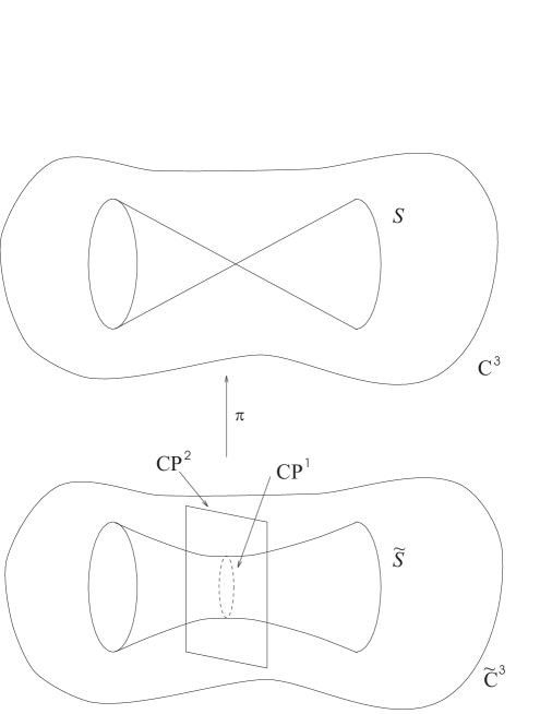
Figure 2.1: The blow-up of $\mathbb{C}^{2}/\mathbb{Z}_{2}$.

As the example of the resolution of $\mathbb{C}^{2}/\mathbb{Z}_{2}$ is very important, we want to look at it from yet another perspective. To do so we need to give the definition of a cone.

Definition 2.6
Let $(M,g)$ be a Riemannian $n$-manifold. A point $p\in M$ is said to be a conical singularity in $M$ if there is a neighbourhood $U_{p}$ of $p$ such that on $U_{p}\backslash\{p\}$ the metric takes the form

$$ds^{2}=dr^{2}+r^{2}d\Omega_{N}^{2}.$$ (2.6)

Here $d\Omega_{N}^{2}$ is a metric on an $(n-1)$-dimensional manifold $N$. If $g$ can be globally written in the form (2.6) $M$ is said to be a cone on $N$. Note that $\mathbb{R}^{n+1}$ can be regarded as a cone on $S^{n}$ with $d\Omega_{N}^{2}$ the standard round metric on $S^{n}$. In that case, of course, we only have a coordinate singularity at $r=0$. In all other cases we have a real singularity in $M$.

Certainly, $S\cong\mathbb{C}^{2}/\mathbb{Z}_{2}$ is a cone over $S^{3}/\mathbb{Z}_{2}$, as $\mathbb{C}^{2}$ is a cone over $S^{3}$. With the special $\mathbb{Z}_{2}$ defined above, $S^{3}/\mathbb{Z}_{2}$ is actually smooth, as the $\mathbb{Z}_{2}$ does not have fixed points in $S^{3}$. In fact, it identifies two antipodal points of the sphere $S^{3}$, so we see that $S^{3}/\mathbb{Z}_{2}$ is actually isomorphic to $SO(3)$. Let us introduce a coordinate $r$ given by $r^{2}:=\sum_{i=0}^{2}|z_{i}|^{2}$. It is important to note that on the blow-up $\widetilde{S}$ there is a smallest value of $r$, which is bigger than zero. It is the radius of the sphere $S^{2}$ sitting in the center of $\widetilde{S}$. We denote this radius $r_{0}$. Of course, the resolution $\widetilde{S}$ no longer is a cone over $S^{3}/\mathbb{Z}_{2}$, but for large $r$ $\widetilde{S}$ tends to $S$, so $\widetilde{S}$ is asymptotically conical. Now consider $SO(3)$ as a $U(1)$-bundle over $S^{2}$. Then the resolved space can be viewed as shown in figure 2.2.

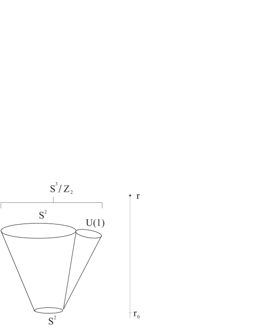
Figure 2.2: Another picture of the resolved space $\widetilde{S}$.

We see that the $U(1)$ fibre collapses as $r$ goes to $r_{0}$ but we are left with an uncollapsed $S^{2}$. In the singular space this $S^{2}$ collapses as well.
We mentioned above that the physical picture of a blow-up is that we first cut out the singularity and then glue in a smooth space instead. In our example this smooth space is called Eguchi-Hanson space $\mathbb{EH}$. Its metric is given by

$$ds^{2}_{\mathbb{EH}}={1\over{1-\left({r_{0}\over r}\right)^{4}}}dr^{2}+r^{2}\left(\sigma_{x}^{2}+\sigma_{y}^{2}+\left(1-\left({r_{0}\over r}\right)^{4}\right)\sigma_{z}^{2}\right),$$ (2.7)

with $r_{0}\in\mathbb{R}^{+}$ a parameter and

$$\sigma_{x} = \cos\psi\,d\theta+\sin\psi\sin\theta\,d\phi,$$

$$\sigma_{y} = -\sin\psi\,d\theta+\cos\psi\sin\theta\,d\phi,$$ (2.8)

$$\sigma_{z} = d\psi+\cos\theta\,d\phi.$$

These $\sigma_{i}$ are invariant under the left action of $SU(2)$ on $S^{3}\cong SU(2)$. Furthermore, it is easy to check that they satisfy $d\sigma_{i}=-\epsilon_{ijk}\sigma_{j}\wedge\sigma_{k}$.
The range of coordinates in (2.7) is $r_{0}\leq r<\infty$, $0\leq\psi<2\pi$, $0\leq\theta\leq\pi$ and $0\leq\phi<2\pi$. Note that the metrics on $S^{2}$ and $S^{3}$ can be written as

$$ds^{2}_{S^{2}} = \sigma_{x}^{2}+\sigma_{y}^{2},$$ (2.9)

$$ds^{2}_{S^{3}} = \sigma_{x}^{2}+\sigma_{y}^{2}+\sigma_{z}^{2}.$$ (2.10)

The entire sphere $S^{3}$ is covered if $\theta$ and $\phi$ range as above, but $0\leq\psi<4\pi$. Thus, we see that for large $r$ the Eguchi-Hanson space is asymptotic to a cone on $S^{3}/\mathbb{Z}_{2}$, as the $\mathbb{Z}_{2}$ acts on $S^{3}$ via $\psi\rightarrow\psi+2\pi$. So topologically a surface of constant $r$ in Eguchi-Hanson space is $S^{3}/\mathbb{Z}_{2}$ and it is possible to excise the singularity of $\mathbb{C}^{2}/\mathbb{Z}_{2}$ and glue in an Eguchi-Hanson space. Details on this procedure can be found in [63]. Note also that for $r=r_{0}$ we find the $S^{2}$ sitting on the tip of the Eguchi-Hanson space.
Finally we want to mention already at this point that $\mathbb{EH}$ is Ricci flat and its holonomy group is $SU(2)$.

2.2 The $K3$ Surface

A complex manifold that turns up again and again in string and M-theory is the $K3$ surface. In this section we give its definition and basic properties as well as some examples.

Definition 2.7
A vector bundle $E$ whose fibre $F$ is one-dimensional is called a line bundle.
A holomorphic vector bundle $E$ on a complex manifold $M$ with fibre $\mathbb{C}$ is called a holomorphic line bundle.
Let $M$ be a complex manifold of dimension $m$, then $\Lambda^{m,0}M$ is a holomorphic line bundle, called the canonical bundle $K_{M}$. It is the bundle of complex volume forms on $M$.

Definition 2.8
A $K3$ surface is a compact, complex surface $(X,J)$ with $h^{1,0}(X)=0$ and trivial canonical bundle.

A simple example of a $K3$ surface is given by the so called Fermat quartic

$$FQ:=\{[z_{0},\ldots,z_{3}]\in\mathbb{CP}^{3}:z_{0}^{4}+z_{1}^{4}+z_{2}^{4}+z_{3}^{4}=0\}.$$ (2.11)

The proof can be found in [63].

Another interesting example is the following. Let $\Lambda\cong\mathbb{Z}^{4}$ be a lattice in $\mathbb{C}^{2}$. Then $\mathbb{C}^{2}/\Lambda\cong T^{4}$. Define a map $\sigma:T^{4}\rightarrow T^{4}$ by $\sigma(z^{1},z^{2}):=(-z^{1},-z^{2})$. Obviously this map has 16 fixed points. Thus $T^{4}/\langle\sigma\rangle$ is a complex orbifold with 16 singularities which are locally isomorphic to $\mathbb{C}^{2}/\mathbb{Z}_{2}$. Each of these singularities can be resolved as we showed above. Define $\widetilde{T^{4}/\langle\sigma\rangle}$ to be the space resulting from blowing up all the singularities. Then $\widetilde{T^{4}/\langle\sigma\rangle}$ is a $K3$ surface [63].

Next we list some important properties of $K3$ surfaces, which are crucial to understand various duality conjectures.

Proposition 2.9
Let $X$ be a $K3$ surface. Then its Betti numbers are $b^{0}=b^{4}=1$, $b^{1}=b^{3}=0$ and $b^{2}=22$. Its Hodge numbers are $h^{0,2}=h^{2,0}=1$ and $h^{1,1}=20$.

From our resolution of a singularity using an Eguchi-Hanson space the number of two-cycles of $K3$ can easily be determined. The number of two-cycles of $T^{4}$ is 6 and these are not effected by the $\mathbb{Z}_{2}$. $T^{4}/\langle\sigma\rangle$ has 16 singularities which are substituted by an Eguchi-Hanson space with a sphere $S^{2}$ on its tip. This increases the number of two-cycles by 16 and we get $b_{2}=b^{2}=22$. This result holds for any $K3$ surface, as one can show that all $K3$ surfaces are homeomorphic.

Proposition 2.10
The moduli space $\mathcal{M}(K3)$ of Einstein metrics on a K3 surface $S$ is given by [83], [11]

$$\mathcal{M}(K3)=\mathbb{R}^{+}\times\left(SO(19,3;\mathbb{Z})\backslash SO(19,3;\mathbb{R})/(SO(19)\times SO(3))\right).$$ (2.12)

Any Einstein metric on K3 is Ricci flat [56].

2.3 Holonomy Groups

The topic of holonomy is a rich one. Holonomy groups can be defined on vector bundles as well as principal bundles, they are related to concepts as different as the topology and the curvature of a manifold. Given the limitations of space, we only present the definition for vector bundles. A case of particular interest is the tangent bundle of a Riemannian manifold, equipped with the Levi-Civita connection. In this special case we speak of Riemannian holonomy groups.

Definition 2.11
Let $M$ be a manifold, $E$ a vector bundle over $M$, and $\nabla^{E}$ a connection on $E$. Fix a point $p\in M$. If $\gamma$ is a loop based at $p$ (i.e. $\gamma(0)=\gamma(1)=p$), then the parallel transport map $P_{\gamma}:E_{p}\rightarrow E_{p}$ is an invertible linear map, so that $P_{\gamma}$ lies in $GL(E_{p})$, the group of invertible linear transformations of $E_{p}$. Define the holonomy group $Hol_{p}(\nabla^{E})$ of $\nabla^{E}$ based at $p$ to be

$$Hol_{p}(\nabla^{E}):=\{P_{\gamma}|\ \gamma\ \mbox{is a loop based at}\ p\}\subset GL(E_{p}).$$

Proposition 2.12
Let $M$ be a connected manifold. Then the holonomy group is independent of $p\in M$ and we denote $Hol(\nabla^{E}):=Hol_{p}(\nabla^{E})$.

Definition 2.13
Let $(M,g)$ be a Riemannian manifold with Levi-Civita connection $\nabla$. Define the holonomy group $Hol(g)$ of $g$ to be $Hol(\nabla)$. Then $Hol(g)$ is a subgroup of $O(n)$, called the Riemannian holonomy group.

The following proposition - which can be easily understood geometrically - clarifies the intimate relation between holonomy and curvature.

Proposition 2.14
Let $M$ be a manifold, $E$ a vector bundle over $M$ and $\nabla^{E}$ a connection on $E$. If $\nabla^{E}$ is flat, so that $R(\nabla^{E})=0$ then $Hol(\nabla^{E})=\{1\}$.

Another proposition relating curvature and holonomy that will be useful later on is the following.

Proposition 2.15
Let $M$ be a manifold, $E$ a vector bundle over $M$, and $\nabla^{E}$ a connection on $E$. Then for each $p\in M$ the curvature $R(\nabla^{E})_{p}$ of $\nabla^{E}$ at $p$ lies in $\verb"hol"_{p}(\nabla^{E})\otimes\Lambda^{2}T^{*}_{p}M$, where $\verb"hol"_{p}(\nabla^{E})$ is the Lie algebra of the holonomy group $Hol_{p}(\nabla^{E})$.

This proposition is the mathematical formulation of formula (D.10) given in the appendix. In particular, we see that $R_{MNAB}\Gamma^{AB}$ is the generator of the holonomy group acting on the spin bundle.

In order to understand the definition of a $G_{2}$-manifold, that will be given below, we need to introduce the concept of $G$-structures.

Definition 2.16
Let $M$ be a manifold of dimension $n$, and $F$ the frame bundle over $M$. Then $F$ is a principal bundle over $M$ with fibre $GL(n,\mathbb{R})$. Let $G$ be a Lie subgroup of $GL(n,\mathbb{R})$. Then a G-structure on $M$ is a principal subbundle $P$ of $F$, with fibre $G$.

The classification of Riemannian holonomy groups

Definition 2.17
Let $M$ be a manifold with $p\in M$ and let $G$ be a Lie group acting on $M$ from the left. The orbit of $p$ under this action is defined as

$$Gp:=\{gp:g\in G\}.$$

Definition 2.18
Let $M$ be a manifold and let $G$ be a Lie group acting on $M$ from the left. The action is called transitive if $\forall p_{1},p_{2}\in M\ \exists g\in G$, such that $gp_{1}=p_{2}$.

Definition 2.19
Let $M$ be a manifold with $p\in M$ and let $G$ be a Lie group acting on M from the left. The isotropy group (little group, stabilizer) of $p$ is a subgroup of $G$ defined by

$$H(p):=\{g\in G:gp=p\}.$$

Often the isotropy group is independent of $p$ and will be denoted $H$ in that case.

Proposition 2.20
Let $G$ be a Lie group and $H$ a Lie subgroup of $G$. The coset space $G/H$ is a manifold called a homogeneous space.
Its dimension is given by ${\rm dim}\ (G/H)={\rm dim}\ G-{\rm dim}\ H$.

Let $(M,g)$ be a symmetric Riemannian manifold, let $G$ be (a subgroup of) the group of isometries acting transitively on $M$ from the left and let $H$ be its isotropy group. Then we have $M\cong G/H$. Note that we sometimes have to take a subgroup of the isometry group to establish the isomorphism. Precise definitions of symmetric spaces and the required properties of $G$ can be found in [63]. In that case the holonomy group of $M$ can be shown to be

$$Hol(g)=H.$$ (2.13)

As an example let us consider the sphere $S^{n}$. Clearly its isometry group is $SO(n+1)$, its isotropy group is $SO(n)$, we have the isomorphism $S^{n}\cong SO(n+1)/SO(n)$ and the holonomy group is $SO(n)$.
Given these properties we can construct spaces carrying particular holonomy groups. In fact, a classification of the holonomy groups of symmetric spaces was found by Cartan. However, the classification of the holonomy groups of nonsymmetric spaces is rather interesting. The question which subgroups of $O(n)$ can be the holonomy group of a non-symmetric Riemannian $n$-manifold $M$ was answered by Berger [18], who proved the following theorem.

Theorem 2.21 (Berger)
Let $M$ be a simply connected manifold of dimension $n$, $g$ a Riemannian metric on $M$ that is irreducible and nonsymmetric. Then exactly one of the following cases holds.

(i) $Hol(g)=SO(n)$ (ii) $n=2m$ with $m\geq 2$, and $Hol(g)=U(m)$ in $SO(2m)$, (iii) $n=2m$ with $m\geq 2$, and $Hol(g)=SU(m)$ in $SO(2m)$, (iv) $n=4m$ with $m\geq 2$, and $Hol(g)=Sp(m)$ in $SO(4m)$, (v) $n=4m$ with $m\geq 2$, and $Hol(g)=Sp(m)Sp(1)$ in $SO(4m)$, (vi) $n=7$ and $Hol(g)=G_{2}$ in $SO(7)$, (vii) $n=8$ and $Hol(g)=Spin(7)$ in $SO(8)$.

$K3$ is an example for spaces with holonomy $SU(2)$. Because the groups $G_{2}$ and $Spin(7)$ are the exceptional cases in this classification, they are referred to as exceptional holonomy groups. The first examples of complete metrics with holonomy $G_{2}$ and $Spin(7)$ on non-compact manifolds were given by Bryant and Salomon in [26] and by Gibbons, Page and Pope in [49]. Compact manifolds with holonomy $G_{2}$ and $Spin(7)$ were constructed by Joyce [60], [61], [62], [63], however, no explicit metric is known.

2.4 Spinors and Holonomy Groups

The objective of compactifying M-theory is to obtain a four-dimensional gauge theory with $\mathcal{N}=1$ supersymmetry. This is equivalent to the existence of a covariantly constant spinor on the compact manifold, as will be shown below. The theorem in this subsection points out that in order to satisfy this requirement the compact manifold must have holonomy group $G_{2}$. This is the reason why physicists have been studying $G_{2}$-manifolds over the last years.
The concept of a spinor is defined in appendix B, the spin connection $\nabla^{S}$ is introduced in appendix D. Contrary to the discussion in the appendix we now take the metric on the base manifold $M$ to have signature $+,\ldots,+$, as we want to compactify on Euclidean manifolds later on. $S$ is the spin bundle over $M$ and $C^{\infty}(S)$ denotes the set of sections of $S$.

Definition 2.22
Take a spinor $\eta\in C^{\infty}(S)$. $\eta$ is called a parallel spinor or (covariantly) constant spinor, if $\nabla^{S}\eta=0$.

In chapter 5 we will relate the number of unbroken supersymmetry after compactification to the number of covariantly constant spinors of the compact space. Hence, the following theorem is of fundamental importance.

Theorem 2.23
Let $M$ be an orientable, connected, simply connected spin $n$-manifold for $n\geq 3$, and $g$ an irreducible Riemannian metric on $M$. Define $N$ to be the dimension of the space of parallel spinors on $M$. If $n$ is even, define $N_{\pm}$ to be the dimension of the space of parallel spinors in $C^{\infty}(S_{\pm})$, so that $N=N_{+}+N_{-}$.
Suppose $N\geq 1$. Then, after making an appropriate choice of orientation for $M$, exactly one of the following holds:

(i) $n=4m$ for $m\geq 1$ and $Hol(g)=SU(2m)$, with $N_{+}=2$ and $N_{-}=0$, (ii) $n=4m$ for $m\geq 2$ and $Hol(g)=Sp(m)$, with $N_{+}=m+1$ and $N_{-}=0$, (iii) $n=4m+2$ for $m\geq 1$ and $Hol(g)=SU(2m+1)$, with $N_{+}=1$ and $N_{-}=1$, (iv) $n=7$ and $Hol(g)=G_{2}$, with $N=1$, (v) $n=8$ and $Hol(g)=Spin(7)$ with $N_{+}=1$ and $N_{-}=0$.

With the opposite orientation, the values of $N_{\pm}$ are exchanged.

In particular, we note that the requirement of a one-dimensional space of covariantly constant spinors on a seven-manifold leads to a manifold with $Hol(g)=G_{2}$.

2.5 The Group $G_{2}$ and the Concept of $G_{2}$-Manifolds

In this section we give the definition of $G_{2}$-manifolds and collect a number of their properties. We define some useful concepts related to them and study three explicit examples.

Definition 2.24
Let $(x_{1},\ldots,x_{7})$ be coordinates on $\mathbb{R}^{7}$. Write $d{\bf x}_{ij\ldots l}$ for the exterior form $dx_{i}\wedge dx_{j}\wedge\ldots\wedge dx_{l}$ on $\mathbb{R}^{7}$. Define a three-form $\varphi_{0}$ on $\mathbb{R}^{7}$ by

$$\varphi_{0}:=d\textbf{x}_{123}+d\textbf{x}_{145}+d\textbf{x}_{167}+d\textbf{x}_{246}-d\textbf{x}_{257}-d\textbf{x}_{347}-d\textbf{x}_{356}.$$ (2.14)

The subgroup of $GL(7,\mathbb{R})$ preserving $\varphi_{0}$ is the exceptional Lie group $G_{2}$. It is compact, connected, simply connected, semisimple and 14-dimensional, and it also fixes the four-form

$$*\varphi_{0}=d{\bf x}_{4567}+d{\bf x}_{2367}+d{\bf x}_{2345}+d{\bf x}_{1357}-d{\bf x}_{1346}-d{\bf x}_{1256}-d{\bf x}_{1247},$$ (2.15)

the Euclidean metric $g_{0}=dx_{1}^{2}+\ldots dx_{7}^{2}$, and the orientation on $\mathbb{R}^{7}$.

Definition 2.25
A $G_{2}$-structure on a seven-manifold $M$ is a principal subbundle of the frame bundle of $M$ with structure group $G_{2}$. Each $G_{2}$-structure gives rise to a 3-form $\varphi$ and a metric $g$ on $M$, such that every tangent space of $M$ admits an isomorphism with $\mathbb{R}^{7}$ identifying $\varphi$ and $g$ with $\varphi_{0}$ and $g_{0}$, respectively. We will refer to $(\varphi,g)$ as a $G_{2}$-structure.
Let $\nabla$ be the Levi-Civita connection, then $\nabla\varphi$ is called the torsion of $(\varphi,g)$. If $\nabla\varphi=0$ then $(\varphi,g)$ is called torsion free.
A $G_{2}$-manifold is defined as the triple $(M,\varphi,g)$, where $M$ is a seven-manifold, and $(\varphi,g)$ a torsion-free $G_{2}$-structure on $M$.

Proposition 2.26
Let $M$ be a seven-manifold and $(\varphi,g)$ a $G_{2}$-structure on $M$. Then the following are equivalent:

(i) $(\varphi,g)$ is torsion-free, (ii) $\nabla\varphi=0$ on $M$, where $\nabla$ is the Levi-Civita connection of $g$, (iii) $d\varphi=d*\varphi=0$ on $M$, (iv) $Hol(g)\subseteq G_{2}$, and $\varphi$ is the induced three-form.

Note that the holonomy group of a $G_{2}$-manifold is not necessarily $G_{2}$.

Properties of $G_{2}$-manifolds

Proposition 2.27
Let $(M,g)$ be a Riemannian manifold with $Hol(g)=G_{2}$. Then $M$ is a spin manifold and the space of parallel spinors has dimension one, as stated above.

Proposition 2.28
Let $(M,g)$ be a Riemannian seven-manifold. If $Hol(g)\subseteq G_{2}$, then $g$ is Ricci-flat.

To prove this we note that we have at least one covariantly constant spinor $\nabla^{S}\eta=0$. But then we know that $0=[\nabla^{S}_{m},\nabla^{S}_{n}]\eta={1\over 4}R_{mnpq}\Gamma^{pq}\eta$ where we used (D.13). Now multiply by $\Gamma^{n}$ to get

$$R_{mnpq}\Gamma^{n}\Gamma^{pq}\eta = 0,$$

$$\Rightarrow\ \ R_{m(npq)}\Gamma^{n}\Gamma^{pq}\eta = 0,\ \ \mbox{as}\ \ R_{m[npq]}=0$$

$$\Rightarrow\ \ \ \ \ \ \ \ \ \mathcal{R}_{mn}\Gamma^{n}\eta = 0,$$

$$\Rightarrow\ \ \ \ \ \ \ \ \ \ \ \ \ \ \mathcal{R}_{mn} = 0,$$

where we used $\Gamma^{n}\Gamma^{pq}=\Gamma^{npq}-\Gamma^{p}\delta^{nq}+\Gamma^{q}\delta^{pn}$.

Proposition 2.29
Let $(M,g)$ be a compact Riemannian manifold with $Hol(g)=G_{2}$, then $H^{1}(M,\mathbb{R})=\{0\}$, so that $b^{1}(M)=0$.

This proposition together with the connectedness of $(M,g)$ and the Poincaré duality enables us to write down the Betti numbers of a compact manifold with holonomy $G_{2}$. They are $b^{0}=b^{7}=1$, $b^{1}=b^{6}=0$ and $b^{2}=b^{5}$ and $b^{3}=b^{4}$ arbitrary.

Proposition 2.30
Let $(M,\varphi,g)$ be a compact $G_{2}$-manifold. Then $Hol(g)=G_{2}$ if and only if $\pi_{1}(M)$ is finite.

Proposition 2.31
Let $M$ be a compact $G_{2}$-manifold with $Hol(g)=G_{2}$. Then the isometry group of $M$ is trivial.

This will be proved in section 5.3.

Proposition 2.32
Let $(M,\varphi,g)$ be a $G_{2}$-manifold. Then $\Lambda^{k}T^{*}M$ splits orthogonally into components. In particular,

$$\Lambda^{3}T^{*}M=\Lambda^{3}_{1}\oplus\Lambda^{3}_{7}\oplus\Lambda^{3}_{27},$$ (2.16)

where $\Lambda^{k}_{l}$ corresponds to an irreducible representation of $G_{2}$ of dimension $l$. This splitting is the only one we need. The other splittings and more details can be found in [63].

Definition 2.33
Let $M$ be an oriented seven-manifold. For each $p\in M$, define $\mathcal{P}^{3}_{p}M$ to be the subset of three-forms $\varphi\in\Lambda^{3}T^{*}M$ for which there exists an oriented isomorphism between $T_{p}M$ an $\mathbb{R}^{7}$ identifying $\varphi$ and $\varphi_{0}$ of (2.14). Define

$$\mathcal{X}:=\{\varphi\in C^{\infty}(\mathcal{P}^{3}M):d\varphi=d*\varphi=0\}.$$ (2.17)

Let $\mathcal{D}$ be the group of all diffeomorphisms $\Psi$ of $M$ isotopic to the identity. Then $\mathcal{D}$ acts naturally on $C^{\infty}(\mathcal{P}^{3}M)$ and $\mathcal{X}$ by $\varphi\stackrel{{\scriptstyle\Psi}}{{\rightarrow}}\Psi_{*}(\varphi)$. Define the moduli space of torsion free $G_{2}$-structures on M to be $\mathcal{M}:=\mathcal{X}/\mathcal{D}$.

Proposition 2.34
Let $M$ be a compact seven-manifold, and $\mathcal{M}=\mathcal{X}/\mathcal{D}$ the moduli space of $G_{2}$-structures on $M$. Then $\mathcal{M}$ is a smooth manifold of dimension $b^{3}(M)$.

Calibrated geometry and $G_{2}$-manifolds

Definition 2.35
Let $(M,g)$ be a Riemannian manifold. An oriented tangent $k$-plane $V$ on $M$ is a vector subspace $V$ of some tangent space $T_{p}M$ to $M$ with dim$V=k$, equipped with an orientation. If $V$ is an oriented tangent $k$-plane on $M$ then $g|_{V}$ is a Euclidean metric on $V$, so combining $g|_{V}$ with the orientation on $V$ gives a natural volume form ${\rm vol}_{V}$ on $V$, which is a $k$-form on $V$.
Now let $\varphi$ be a closed $k$-form on $M$. We say that $\varphi$ is a calibration on $M$ if for every oriented $k$-plane $V$ on $M$ we have $\varphi|_{V}\leq{\rm vol}_{V}$. Here $\varphi|_{V}=\alpha\cdot{\rm vol}_{V}$ for some $\alpha\in\mathbb{R}$ and $\varphi|_{V}\leq{\rm vol}_{V}$ if $\alpha\leq 1$. Let $N$ be an oriented submanifold of $M$ with dimension $k$. Then each tangent space $T_{p}N$ for $p\in N$ is an oriented tangent $k$-plane. We say that $N$ is a calibrated submanifold if $\varphi|_{T_{p}N}={\rm vol}_{T_{p}N}$ for all $p\in N$.

Proposition 2.36
Let $(M,g)$ be a Riemannian manifold, $\varphi$ a calibration on $M$, and $N$ a compact calibrated submanifold in $M$. Then $N$ is volume minimizing in its homology class.

To prove this we denote $k:=dim(N)$, and let $[N]\in H_{k}(M,\mathbb{R})$ and $[\varphi]\in H^{k}(M,\mathbb{R})$ be the homology and cohomology classes of $N$ and $\varphi$. Then

$$[\varphi]\cdot[N]=\int_{x\in N}\varphi|_{T_{x}N}=\int_{x\in N}{\rm vol}_{T_{x}N}={\rm vol}(N),$$

since $\varphi_{T_{x}N}={\rm vol}_{T_{x}N}$. If $N^{\prime}$ is any other compact $k$-submanifold of $M$ with $[N^{\prime}]=[N]$ in $H_{k}(M,\mathbb{R})$, then

$$[\varphi]\cdot[N]=[\varphi]\cdot[N^{\prime}]=\int_{x\in N^{\prime}}\varphi|_{T_{x}N^{\prime}}\leq\int_{x\in N^{\prime}}{\rm vol}_{T_{x}N^{\prime}}={\rm vol}(N^{\prime}),$$

since $\varphi|_{T_{x}N^{\prime}}\leq{\rm vol}_{T_{x}N^{\prime}}$ because $\varphi$ is a calibration. Thus, ${\rm vol}(N^{\prime})\leq{\rm vol}(N)$.

A Riemannian manifold $(M,g)$ with holonomy $G_{2}$ defines a three-form $\varphi$ and a four-form $\star\varphi$, as given above. These are both calibrations. Calibrated submanifolds with respect to $\varphi$ are called associative three-folds, calibrated submanifolds with respect to $\star\varphi$ are called co-associative four-folds.
The general relation between calibrations and holonomy groups can be found in [63].

Weak $G_{2}$

There is yet another notion which is important for M-theory compactifications, namely that of weak $G_{2}$-holonomy, or a nearly parallel $G_{2}$-structure [47], [50]. These are $G_{2}$-structures $(\varphi,g)$ with a Killing spinor, rather than a constant spinor. That is we have $\nabla^{S}\eta=i{\lambda\over 2}\gamma\eta$. On such manifolds the three-form satisfies $d\varphi=4\lambda*\varphi$ and $d*\varphi=0$, for some $\lambda\in\mathbb{R}$ and they are automatically Einstein with non-negative scalar curvature $6\lambda^{2}$. In the case of $\lambda=0$ we get a $G_{2}$-manifold. Explicit metrics of compact weak $G_{2}$-manifolds with conical singularities were first constructed in [22].

Examples of $G_{2}$ manifolds

Compact $G_{2}$-manifolds are complicated objects and have been constructed only recently. We present the simplest construction of such a manifold following the general construction mechanism presented by Joyce [63]. The basic tack is a follows. We start with a torus $T^{7}$, equipped with a flat $G_{2}$-structure $(\varphi_{0},g_{0})$ and a finite group $\Gamma$ of automorphisms of $T^{7}$ preserving $(\varphi_{0},g_{0})$. Then $T^{7}/\Gamma$ is an orbifold with a flat $G_{2}$-structure. This orbifold can be resolved and deformed to a smooth compact manifold of holonomy $G_{2}$. The resulting manifold depends on the choice of the group $\Gamma$ and the way of resolving the orbifold. Various different $G_{2}$-manifolds can be constructed in that way.
After having analyzed the simplest example we will move on to the more complicated manifolds which will play an important role in M-theory compactifications.

Example 1
For our first example let $(x_{1},x_{2},x_{3},x_{4},x_{5},x_{6},x_{7})$ be coordinates on $\mathbb{R}^{7}$, and let $(\varphi_{0},g_{0})$ be the flat $G_{2}$-structure on $\mathbb{R}^{7}$, i.e.

$$\varphi_{0} := d\textbf{x}_{123}+d\textbf{x}_{145}+d\textbf{x}_{167}+d\textbf{x}_{246}-d\textbf{x}_{257}-d\textbf{x}_{347}-d\textbf{x}_{356},$$

$$g_{0} = dx_{1}^{2}+\ldots+dx_{7}^{2}.$$

Let $\mathbb{Z}^{7}$ act on $\mathbb{R}^{7}$ by translation in the obvious way, and let $T^{7}:=\left(\mathbb{R}/\mathbb{Z}\right)^{7}$. Then $(\varphi_{0},g_{0})$ can be pulled back on $T^{7}$. We take $([x_{1}],[x_{2}],[x_{3}],[x_{4}],[x_{5}],[x_{6}],[x_{7}])$ to be coordinates on $T^{7}$, where $[x_{i}]:=x_{i}+\mathbb{Z}$.
To proceed we define the maps $\alpha,\beta,\gamma:T^{7}\rightarrow T^{7}$ by

$$\alpha([x_{1}],[x_{2}],[x_{3}],[x_{4}],[x_{5}],[x_{6}],[x_{7}]) = ([x_{1}],[x_{2}],[x_{3}],[-x_{4}],[-x_{5}],[-x_{6}],[-x_{7}]),$$

$$\beta([x_{1}],[x_{2}],[x_{3}],[x_{4}],[x_{5}],[x_{6}],[x_{7}]) = ([x_{1}],[-x_{2}],[-x_{3}],[x_{4}],[x_{5}],[{1\over 2}-x_{6}],[-x_{7}]),$$

$$\gamma([x_{1}],[x_{2}],[x_{3}],[x_{4}],[x_{5}],[x_{6}],[x_{7}]) = ([-x_{1}],[x_{2}],[-x_{3}],[x_{4}],[{1\over 2}-x_{5}],[x_{6}],[{1\over 2}-x_{7}]).$$

Obviously these maps preserve $\varphi_{0}$ and $g_{0}$, therefore, $\Gamma:=\langle\alpha,\beta,\gamma\rangle$ is a group of isometries of $T^{7}$ preserving the flat $G_{2}$-structure $(\varphi_{0},g_{0})$. Furthermore they certainly are involutions, $\alpha^{2}=\beta^{2}=\gamma^{2}=1$, and $\alpha,\beta,\gamma$ commute, e.g.

$$(\alpha\circ\beta - \beta\circ\alpha)([x_{1}],[x_{2}],[x_{3}],[x_{4}],[x_{5}],[x_{6}],[x_{7}])$$

$$= \alpha([x_{1}],[-x_{2}],[-x_{3}],[x_{4}],[x_{5}],[{1\over 2}-x_{6}],[-x_{7}])$$

$$-\beta([x_{1}],[x_{2}],[x_{3}],[-x_{4}],[-x_{5}],[-x_{6}],[-x_{7}])$$

$$= ([x_{1}],[-x_{2}],[-x_{3}],[-x_{4}],[-x_{5}],[x_{6}-{1\over 2}],[x_{7}])$$

$$-([x_{1}],[-x_{2}],[-x_{3}],[-x_{4}],[-x_{5}],[{1\over 2}+x_{6}],[x_{7}])$$

$$= ([0],[0],[0],[0],[0],[-1],[0])=0,$$

and similarly for all other commutators. Collecting all these results we find the isomorphism $\Gamma\cong\mathbb{Z}_{2}^{3}$.
Next we want to analyze the set $T^{7}/\Gamma$, in particular we are interested in its singularities. To do so we list the elements of $\Gamma$ explicitly,

$$\Gamma = \{1,\alpha,\beta,\gamma,\alpha\beta,\alpha\gamma,\beta\gamma,\alpha\beta\gamma\},$$

$$\alpha\beta = ([x_{1}],[-x_{2}],[-x_{3}],[-x_{4}],[-x_{5}],[x_{6}-{1\over 2}],[x_{7}]),$$

$$\alpha\gamma = ([-x_{1}],[x_{2}],[-x_{3}],[-x_{4}],[x_{5}-{1\over 2}],[-x_{6}],[x_{7}-{1\over 2}]),$$

$$\beta\gamma = ([-x_{1}],[-x_{2}],[x_{3}],[x_{4}],[{1\over 2}-x_{5}],[{1\over 2}-x_{6}],[x_{7}-{1\over 2}]),$$

$$\alpha\beta\gamma = ([-x_{1}],[-x_{2}],[x_{3}],[-x_{4}],[x_{5}-{1\over 2}],[x_{6}-{1\over 2}],[{1\over 2}-x_{7}]).$$

In particular, we see that $\alpha\beta$, $\alpha\gamma$, $\beta\gamma$ and $\alpha\beta\gamma$ have no fixed points, as e.g. $[x_{6}]\stackrel{{\scriptstyle\alpha\beta}}{{\rightarrow}}[x_{6}-{1\over 2}]$, $[x_{5}]\stackrel{{\scriptstyle\alpha\gamma}}{{\rightarrow}}[x_{5}-{1\over 2}]$, $[x_{7}]\stackrel{{\scriptstyle\beta\gamma}}{{\rightarrow}}[x_{7}-{1\over 2}]$ and $[x_{5}]\stackrel{{\scriptstyle\alpha\beta\gamma}}{{\rightarrow}}[x_{5}-{1\over 2}]$. Next we analyze the fixed point sets of $\alpha,\beta,\gamma$. Clearly for $x_{4},\ x_{5},\ x_{6},\ x_{7}\in\{\mathbb{Z},\mathbb{Z}+{1\over 2}\}$ $([x_{1}],[x_{2}],[x_{3}],[x_{4}],[x_{5}],[x_{6}],[x_{7}])$ are fixed points of $\alpha$ for any value of $x_{1},\ x_{2},\ x_{3}$. So the fixed point set of $\alpha$ is the union of 16 disjoint copies of $T^{3}$.
Similarly $\beta$ and $\gamma$ have have fixed point sets of 16 tori $T^{3}$. Let us now study the action of $\beta$ on the fixed point set of $\alpha$. Clearly $[x_{4}]\stackrel{{\scriptstyle\beta}}{{\rightarrow}}[x_{4}]$, $[x_{5}]\stackrel{{\scriptstyle\beta}}{{\rightarrow}}[x_{5}]$, $[x_{6}]\stackrel{{\scriptstyle\beta}}{{\rightarrow}}[x_{6}+{1\over 2}]$ and $[x_{7}]\stackrel{{\scriptstyle\beta}}{{\rightarrow}}[x_{7}]$ for $x_{4},\ x_{5},\ x_{6},\ x_{7}\in\{\mathbb{Z},\mathbb{Z}+{1\over 2}\}$. Similarly for $\gamma$, $[x_{4}]\stackrel{{\scriptstyle\gamma}}{{\rightarrow}}[x_{4}]$, $[x_{5}]\stackrel{{\scriptstyle\gamma}}{{\rightarrow}}[x_{5}+{1\over 2}]$, $[x_{6}]\stackrel{{\scriptstyle\gamma}}{{\rightarrow}}[x_{6}]$ and $[x_{7}]\stackrel{{\scriptstyle\gamma}}{{\rightarrow}}[x_{7}+{1\over 2}]$ for $x_{4},\ x_{5},\ x_{6},\ x_{7}\in\{\mathbb{Z},\mathbb{Z}+{1\over 2}\}$ and $\beta\gamma$, $[x_{4}]\stackrel{{\scriptstyle\beta\gamma}}{{\rightarrow}}[x_{4}]$, $[x_{5}]\stackrel{{\scriptstyle\beta\gamma}}{{\rightarrow}}[x_{5}+{1\over 2}]$, $[x_{6}]\stackrel{{\scriptstyle\beta\gamma}}{{\rightarrow}}[x_{6}+{1\over 2}]$ and $[x_{7}]\stackrel{{\scriptstyle\beta\gamma}}{{\rightarrow}}[x_{7}+{1\over 2}]$ for $x_{4},\ x_{5},\ x_{6},\ x_{7}\in\{\mathbb{Z},\mathbb{Z}+{1\over 2}\}$. This implies that the group $\langle\beta,\gamma\rangle$ acts freely on the fixed point set of $\alpha$. Following the same line of arguments we can show that $\langle\alpha,\gamma\rangle$ acts freely on the fixed point set of $\beta$ and $\langle\alpha,\beta\rangle$ acts freely on the fixed point set of $\gamma$. Now we are ready to formulate the following lemma.

Lemma 2.37
The singular set $S$ of $T^{7}/\Gamma$ is a disjoint union of 12 copies of $T^{3}$, and the singularity at each $T^{3}$ is locally modelled by $T^{3}\times\mathbb{C}^{2}/\mathbb{Z}_{2}$.

Let $S^{\prime}$ be the set of fixed points of some non-identity element in $\Gamma$. We know that $S^{\prime}$ is the union of three sets of 16 tori $T^{3}$. To show that $S^{\prime}$ in fact is the disjoint union of 48 tori suppose that two of the sets intersect, say those of $\alpha$ and $\beta$. Then the intersection is fixed by $\alpha$ and $\beta$. But this would imply that $\alpha\beta$ has fixed points, which is wrong.
Now $S=S^{\prime}/\Gamma$ and $\langle\beta,\gamma\rangle$ acts freely on the 16 tori $T^{3}$ fixed by $\alpha$. Therefore these contribute 4 $T^{3}$ to $S$. The same is true for $\beta$ and $\gamma$, so we deduce that $S$ consists of 12 disjoint tori $T^{3}$.
It can be shown [63] that $T^{7}/\Gamma$ is simply connected and has Betti numbers $b^{0}=b^{7}=1$, $b^{1}=b^{2}=b^{5}=b^{6}=0$ and $b^{3}=b^{4}=7$. As was shown by Joyce, $T^{7}/\Gamma$ has a resolution $\widetilde{T^{7}/\Gamma}$ carrying torsion free $G_{2}$-structures. The basic idea is that near a singular $T^{3}$ the orbifold $T^{7}/\Gamma$ looks like $T^{3}\times\mathbb{C}^{2}/\mathbb{Z}_{2}$. For each singularity a copy of $T^{3}\times\mathbb{C}^{2}/\mathbb{Z}_{2}$ is excised and substituted by a space $T^{3}\times\mathbb{EH}$, where $\mathbb{EH}$ is an Eguchi-Hanson space. We saw above that $\mathbb{EH}$ is diffeomorphic to the blow-up at 0 of $\mathbb{C}^{2}/\mathbb{Z}_{2}$. It has Betti numbers $b^{0}=b^{2}=1$ and $b^{1}=b^{3}=b^{4}=0$. One can show that $\pi(\widetilde{T^{7}/\Gamma})\cong\pi(T^{7}/\Gamma)$, so we conclude that $\widetilde{T^{7}/\Gamma}$ is simply connected. From proposition 2.30 we deduce that the manifold $\widetilde{T^{7}/\Gamma}$ has holonomy $G_{2}$. Finally, let us look at the Betti numbers. We have

$$b^{k}(\widetilde{T^{7}/\Gamma})=b^{k}(T^{7}/\Gamma)-12b^{k}(T^{3}\times\mathbb{C}^{2}/\mathbb{Z}_{2})+12b^{k}(T^{3}\times\mathbb{EH}),$$ (2.18)

which is quite intuitive keeping in mind the excision procedure. With $b^{2}(T^{3}\times\mathbb{EH})=b^{3}(T^{3}\times\mathbb{EH})=4$, $b^{2}(T^{3}\times\mathbb{C}^{2}/\mathbb{Z}_{2})=3$ and $b^{3}(T^{3}\times\mathbb{C}^{2}/\mathbb{Z}_{2})=1$ we get

$$b^{2}(\widetilde{T^{7}/\Gamma}) = 12,$$ (2.19)

$$b^{3}(\widetilde{T^{7}/\Gamma}) = 43.$$ (2.20)

So we constructed a compact manifold $\widetilde{T^{7}/\Gamma}$ with holonomy group $G_{2}$ and Betti numbers $b^{2}=12$ and $b^{3}=43$.
This manifold was used in a duality conjecture in string theory in [1].

Example 2
The second example we want to consider has $T^{7}$ and $(\varphi_{0},g_{0})$ as before but this time we define

$$\alpha([x_{1}],[x_{2}],[x_{3}],[x_{4}],[x_{5}],[x_{6}],[x_{7}]) = ([x_{1}],[x_{2}],[x_{3}],[-x_{4}],[-x_{5}],[-x_{6}],[-x_{7}]),$$

$$\beta([x_{1}],[x_{2}],[x_{3}],[x_{4}],[x_{5}],[x_{6}],[x_{7}]) = ([x_{1}],[-x_{2}],[-x_{3}],[x_{4}],[x_{5}],[-x_{6}],[-x_{7}]),$$

$$\gamma([x_{1}],[x_{2}],[x_{3}],[x_{4}],[x_{5}],[x_{6}],[x_{7}]) = ([-x_{1}],[x_{2}],[{1\over 2}-x_{3}],[x_{4}],[-x_{5}],[x_{6}],[-x_{7}]).$$

As before one can show that $\Gamma:=\langle\alpha,\beta,\gamma\rangle$ is isomorphic to $\mathbb{Z}_{2}^{3}$ and that it preserves $(\varphi_{0},g_{0})$. An explicit calculation similar to the one given in our first example yields the following results [63].
The elements $\beta\gamma$ and $\alpha\beta\gamma$ of $\Gamma$ have no fixed points on $T^{7}$. The fixed points of $\alpha$, $\beta$, $\alpha\beta$, $\gamma$ and $\alpha\gamma$ in $T^{7}$ are each 16 copies of $T^{3}$. Moreover $\langle\beta,\gamma\rangle$ acts trivially on the set of 16 $T^{3}$ fixed by $\alpha$, and $\alpha$ acts trivially on the sets of 16 $T^{3}$ fixed by $\beta$, $\alpha\beta$, $\gamma$ and $\alpha\gamma$. The fixed points of $\alpha$, $\beta$ and $\alpha\beta$ intersect in 64 $S^{1}$ in $T^{7}$, the fixed point set of $\langle\alpha,\beta\rangle$. Similarly, the fixed points of $\alpha$, $\gamma$ and $\alpha\gamma$ intersect in 64 $S^{1}$ in $T^{7}$, the fixed point set of $\langle\alpha,\gamma\rangle$.
The fixed point set $S$ of $T^{7}/\Gamma$ is the union of
(i) 16 $T^{3}/\mathbb{Z}^{2}_{2}$ from the $\alpha$ fixed points, (ii) 8 $T^{3}/\mathbb{Z}^{2}_{2}$ from the $\beta$ fixed points, (iii) 8 $T^{3}/\mathbb{Z}^{2}_{2}$ from the $\alpha\beta$ fixed points, (iv) 8 $T^{3}/\mathbb{Z}^{2}_{2}$ from the $\gamma$ fixed points, (v) 8 $T^{3}/\mathbb{Z}^{2}_{2}$ from the $\alpha\gamma$ fixed points.
This union is not disjoint. Instead, the sets (i), (ii) and (iii) intersect in 32 $S^{1}$ in $T^{7}/\Gamma$ from the fixed points of $\langle\alpha,\beta\rangle$ and the sets (i), (iv) and (v) intersect in 32 $S^{1}$ in $T^{7}/\Gamma$ from the fixed points of $\langle\alpha,\gamma\rangle$.
The fixed points of $\langle\alpha,\beta\rangle$ are $\{([x_{1}],\ldots,[x_{7}]):x_{2},\ldots,x_{7}\in\{\mathbb{Z},\mathbb{Z}+{1\over 2}\}\}$. These are 64 copies of $S^{1}$ in $T^{7}$. As $\gamma$ acts freely upon them, their image in $T^{7}/\Gamma$ is 32 $S^{1}$. We shall describe the singularities of $T^{7}/\Gamma$ close to one of these $S^{1}$, say that with $[x_{2}]=\ldots=[x_{7}]=\mathbb{Z}$. Near this $S^{1}$ identify $T^{7}$ with $S^{1}\times\mathbb{C}^{3}$ by equating $([x_{1}],[y_{2}],\ldots,[y_{7}])$ with $([x_{1}],y_{2}+iy_{3},\ldots,y_{6}+iy_{7})$, where $y_{i}$ is small. Then the action of $\alpha$ and $\beta$ on $T^{7}$ can be understood as an action on $S^{1}\times\mathbb{C}^{3}$

$$\alpha([x_{1}],(z_{1},z_{2},z_{3})) = ([x_{1}],(z_{1},-z_{2},-z_{3})),$$ (2.21)

$$\beta([x_{1}],(z_{1},z_{2},z_{3})) = ([x_{1}],(-z_{1},z_{2},-z_{3})).$$ (2.22)

Thus $T^{7}/\Gamma$ is locally isomorphic to $S^{1}\times\mathbb{C}^{3}/\mathbb{Z}_{2}^{2}$.
This kind of singularity can be resolved in various ways. One possibility is to resolve it in two steps. In the first stage we resolve $T^{7}/\langle\alpha\rangle=T^{3}\times T^{4}/\mathbb{Z}_{2}$. The resolution of $T^{4}/\mathbb{Z}_{2}$ is the K3 surface, as we discussed already below definition 2.8, so we get $T^{3}\times K3$. This can be done in a way such that the action of $\langle\beta,\gamma\rangle$ lifts to $T^{3}\times K3$, thus $T^{3}\times K3/\langle\beta,\gamma\rangle$ is an orbifold. Then, in a second step one can resolve the orbifold $T^{3}\times K3/\langle\beta,\gamma\rangle$ to get a smooth $G_{2}$-manifold. To do so one has to analyze the singularities of $T^{3}\times K3/\langle\beta,\gamma\rangle$. It turns out that near the singular points the orbifold is modelled by $\mathbb{R}^{3}\times\mathbb{R}^{4}/\mathbb{Z}_{2}=\mathbb{R}^{3}\times\mathbb{C}^{2}/\mathbb{Z}_{2}=\mathbb{R}^{3}\times\mathbb{C}^{2}/\Gamma_{A_{1}}$. The details of the resolution can be found in [63] and we will not need them in what follows. However, it is important to keep in mind that there exists a singular limit of a smooth compact $G_{2}$-manifold which looks locally like $\mathbb{R}^{3}\times\mathbb{C}^{2}/\Gamma_{A_{1}}$.

Example 3: A non-compact $G_{2}$-manifold
Non-compact $G_{2}$-manifolds were constructed in [26] and [49]. Their structure is less difficult than the one of compact manifolds. In particular, the metric can be written down explicitly.

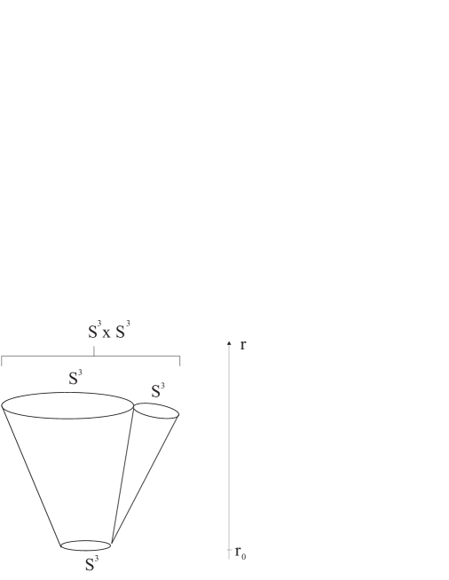
Figure 2.3: A non-compact $G_{2}$-manifold.

One example is a space that is topologically $\mathbb{R}^{4}\times S^{3}\cong\mathbb{C}^{2}\times S^{3}$ and which carries the metric

$$ds_{7}^{2}={1\over 1-\left({r_{0}\over r}\right)^{3}}dr^{2}+{1\over 9}r^{2}\left(1-\left({r_{0}\over r}\right)^{3}\right)(\nu_{1}^{2}+\nu_{2}^{2}+\nu_{3}^{2})+{r^{2}\over 12}(\sigma_{1}^{2}+\sigma_{2}^{2}+\sigma_{3}^{2}).$$ (2.23)

Here $\nu_{i}:=\Sigma_{i}-{1\over 2}\sigma_{i}$ and $\sigma_{i}$ and $\Sigma_{i}$ are left invariant one-forms on two different $S^{3}$’s. For large $r$ the space tends to a cone on $S^{3}\times S^{3}$, so it is asymptotically conical. However, it is not a cone on $S^{3}\times S^{3}$ as for $r=r_{0}$ we get one uncollapsed $S^{3}$, thus there is no singularity. The space is depicted in figure 2.3, its structure is similar to the one of Eguchi-Hanson space. We see that globally it is a fibre bundle over $S^{3}$ with fibres $\mathbb{C}^{2}$. Note that the metric does not involve the standard metric on $S^{3}\times S^{3}$ but rather the homogeneous metric on $SU(2)^{3}/SU(2)_{diag}$. In particular this allows us to define an action of $SU(2)$ on our manifold which keeps fixed the base $S^{3}$ and acts on the fibre $\mathbb{C}^{2}$ in a natural way. These properties will be important in chapter 7.
For a proof that the Levi-Civita connection of this metric really has holonomy $G_{2}$ see [49]. A detailed description of this space can be found in [49] and [12].

Chapter 3 Preliminary Physics

3.1 Eleven-dimensional Supergravity

It is current wisdom in string theory [83] that the low energy limit of M-theory is eleven-dimensional supergravity [31]. Therefore, M-theory results can be found using this well understood supergravity theory. In this section we review the basic field content, the Lagrangian and its symmetries as well as the equations of motion. More details can be found in [77], [34], [35], [40] and [81].

The action of eleven-dimensional supergravity

The field content of eleven-dimensional supergravity is remarkably simple. It consists of the metric $g_{MN}$, a Majorana spin-${3\over 2}$ fermion $\psi_{M}$ and a three-form $C={1\over{3!}}C_{MNP}dz^{M}\wedge dz^{N}\wedge dz^{P}$, where $z^{M}$ is a set of coordinates on the space-time manifold $M_{11}$. These fields can be combined to give the unique $\mathcal{N}=1$ supergravity theory in eleven dimensions. The full action is

$\displaystyle S$ $\displaystyle=$ $\displaystyle{1\over{2\kappa_{11}^{2}}}\int[\mathcal{R}*1-{1\over 2}G\wedge*G-{1\over 6}C\wedge G\wedge G]$ $\displaystyle+{1\over 2\kappa_{11}^{2}}\int d^{11}z\sqrt{g}\bar{\psi}_{M}\Gamma^{MNP}\nabla^{S}_{N}\left({\omega+\hat{\omega}\over 2}\right)\psi_{P}$ $\displaystyle-{1\over 2\kappa_{11}^{2}}{1\over 192}\int d^{11}z\sqrt{g}\left(\bar{\psi}_{M}\Gamma^{MNPQRS}\psi_{N}+12\bar{\psi}^{P}\Gamma^{RS}\psi^{Q}\right)(G_{PQRS}+\hat{G}_{PQRS}).$

The general notation and conventions adopted are given in the appendix. To explain the contents of the action, we start with the commutator of the vielbeins, which defines the anholonomy coefficients $\Omega_{AB}^{\ \ \ \ C}$

$$[e_{A},e_{B}]:=[e^{\ \ M}_{A}\partial_{M},e^{\ \ N}_{B}\partial_{N}]=\Omega_{AB}^{\ \ \ \ C}e_{C}.$$ (3.2)

Relevant formulae for the spin connection are

$$\omega_{MAB}(e) = {1\over 2}(-\Omega_{MAB}+\Omega_{ABM}-\Omega_{BMA})$$

$$\omega_{MAB} = \omega_{MAB}(e)+{1\over 8}[-\bar{\psi}_{P}\Gamma_{MAB}^{\ \ \ \ \ \ PQ}\psi_{Q}+2(\bar{\psi}_{M}\Gamma_{B}\psi_{A}-\bar{\psi}_{M}\Gamma_{A}\psi_{B}+\bar{\psi}_{B}\Gamma_{M}\psi_{A})]$$

$$\hat{\omega}_{MAB} := \omega_{MAB}+{1\over 8}\bar{\psi}_{P}\Gamma_{MAB}^{\ \ \ \ \ \ PQ}\psi_{Q}.$$ (3.3)

$\hat{\omega}$ is the supercovariant connection, whose variation does not involve derivatives of the infinitesimal Grassmann parameter. $\psi_{M}$ is a Majorana vector-spinor. The Lorentz covariant derivative reads

$$\nabla^{S}_{M}(\omega)\psi_{N}=\partial_{M}\psi_{N}+{1\over 4}\omega_{MAB}\Gamma^{AB}\psi_{N}.$$ (3.4)

For further convenience we define

$$\widetilde{\nabla}^{S}_{M}(\omega)\psi_{N}:=\nabla^{S}_{M}(\omega)\psi_{N}-{1\over 288}(\Gamma_{M}^{\ \ PQRS}-8\delta_{M}^{P}\Gamma^{QRS})\hat{G}_{PQRS}\psi_{N}.$$

$$G:=dC\ \ \mbox{i.e.}\ \ G_{MNPQ}=4\partial_{[M}C_{NPQ]}.$$ (3.5)

The supercovariantization $\hat{G}_{MNPQ}$ is defined as a term without derivatives of the infinitesimal parameter in its supersymmetry variation,

$$\hat{G}_{MNPQ}:=G_{MNPQ}+3\bar{\psi}_{[M}\Gamma_{NP}\psi_{Q]}.$$ (3.6)

Symmetries of eleven-dimensional supergravity

The action and equations of motion are invariant under the following symmetries.

a, $d=11$ general covariance (parameter $\xi^{M}$)

$$\delta e_{\ \ M}^{A} = e_{\ \ N}^{A}\partial_{M}\xi^{N}+\xi^{N}\partial_{N}e_{\ \ M}^{A}$$

$$\delta C_{MNP} = 3C_{Q[MN}\partial_{P]}\xi^{Q}+\xi^{Q}\partial_{Q}C_{MNP}$$

$$\delta\psi_{M} = \psi_{N}\partial_{M}\xi^{N}+\xi^{N}\partial_{N}\psi_{M}$$ (3.7)

b, Local $SO(1,10)$ Lorentz transformations (parameter $\alpha_{AB}=-\alpha_{BA}$)

$$\delta e_{\ \ M}^{A} = -\alpha_{\ \ B}^{A}e_{\ \ M}^{B}$$

$$\delta C_{MNP} = 0$$

$$\delta\psi_{M} = -{1\over 4}\alpha_{AB}\Gamma^{AB}\psi_{M}$$ (3.8)

c, $\mathcal{N}=1$ Supersymmetry (parameter $\eta$, anti-commuting)

$$\delta e_{\ \ M}^{A} = -{1\over 2}\bar{\eta}\Gamma^{A}\psi_{M}$$

$$\delta C_{MNP} = -{3\over 2}\bar{\eta}\Gamma_{[MN}\psi_{P]}$$

$$\delta\psi_{M} = \widetilde{\nabla}^{S}_{M}(\hat{\omega})\eta$$ (3.9)

d, Abelian gauge transformations (parameter $\Lambda={1\over 2}\Lambda_{MN}dz^{M}\wedge dz^{n}$)

$$\delta e_{\ \ M}^{A} = 0$$

$$\delta C_{MNP} = 3\partial_{[M}\Lambda_{NP]}\Leftrightarrow\delta C=d\Lambda$$

$$\delta\psi_{M} = 0$$ (3.10)

e, Odd number of space or time reflections together with

$$C_{MNP}\rightarrow-C_{MNP}$$ (3.11)

Field equations of eleven-dimensional supergravity

We will only need solutions of the equations of motion with the property that $\psi_{M}\equiv 0$. Hence we can set $\psi_{M}$ to zero before varying the equations of motion. This leads to an enormous simplification of the calculations. The equations of motion with vanishing fermion field read

$$\mathcal{R}_{MN}(\omega)-{1\over 2}g_{MN}\mathcal{R}(\omega)={1\over 12}\left(G_{MPQR}G_{N}^{\ \ PQR}-{1\over 8}g_{MN}G_{PQRS}G^{PQRS}\right)$$ (3.12)

$$\nabla_{M}G^{MPQR}+{1\over 2\cdot 4!\cdot 4!}\epsilon^{PQRSTUVWXYZ}G_{STUV}G_{WXYZ}=0.$$ (3.13)

The last equation can be rewritten more conveniently in terms of differential forms

$$d*G+{1\over 2}G\wedge G=0.$$ (3.14)

In addition to those field equations we also know that G is closed, as it is exact,

$$dG=0.$$ (3.15)

We note in passing that these equations enable us to define two conserved charges

$$Q_{e}:=\int_{\partial M_{8}}\left(*G+{1\over 2}C\wedge G\right),$$ (3.16)

$$Q_{m}:=\int_{\partial M_{5}}G,$$ (3.17)

where the integrations are over the boundary at infinity of a space-like subspace of eight and five dimensions. Note that these subspaces do not fill out the ten-dimensional space, so the situation is different from Maxwell’s theory in four dimensions.

3.2 Anomalies

In this section we will give the main results on anomalies that will be needed at various places in our analysis of M-theory. We will focus on general aspects of anomalies without reference to their explicit calculation from perturbative quantum field theory. General references for this section are [7], [8], [9], [75] and [76]. Details on the concept of anomaly inflow and anomalies in M-theory can be found in [24].

In order to construct a quantum field theory one usually starts from a classical theory which is quantized by following one of several possible quantization schemes. Therefore, a detailed analysis of the classical theory is a crucial prerequisite for understanding the dynamics of the quantum theory. In particular, the symmetries and the related conservation laws should be mirrored on the quantum level. However, it turns out that this is not always true. If the classical theory possesses a symmetry that cannot be maintained on the quantum level we speak of an anomaly.
To see explicitly how an anomaly can arise it is useful to look at the individual steps involved in the process of quantization. As is well known, many quantum field theories lead to divergences if naive calculations are performed. To get rid of these the theory has to be carefully regularized. If this regularized theory still has the same symmetries as the classical theory no anomalies can occur. This changes, however, if some symmetries cannot be maintained by any regularization scheme. Then we can no longer expect that the corresponding conservation laws hold on the quantum level after the regulator is removed. An explicit check has to be made, using the methods of perturbation theory.

Before discussing anomalies in detail we want to point out the connection between symmetries and conserved currents. A theory containing a massless gauge field $A$ is only consistent if the action is invariant under the infinitesimal local gauge transformation

$$A^{\prime}(x)=A(x)+D\epsilon(x).$$ (3.18)

The invariance of the action can be written as

$$D_{M}(x){{\delta S[A]}\over{\delta A_{aM}(x)}}=0,$$ (3.19)

where $A=A_{a}T_{a}=A_{aM}T_{a}dx^{M}$. Then we can define a current corresponding to this symmetry,

$$J_{a}^{M}(x):={\delta S[A]\over\delta A_{aM}(x)},$$ (3.20)

and gauge invariance (3.19) of the action tells us that this current is conserved,

$$D_{M}J^{M}_{a}(x)=0.$$ (3.21)

If on the other hand a symmetry is violated on the quantum level we can no longer expect that the corresponding current is conserved. Suppose we consider a theory containing massless fermions $\psi$ in the presence of an external gauge field $A$.
In such a case the expectation value of an operator is defined as

$$\langle\mathcal{O}\rangle={\int D\psi D\bar{\psi}\ \mathcal{O}\exp(-S[\psi,A])\over\int D\psi D\bar{\psi}\ \exp(-S[\psi,A])}.$$ (3.22)

We define the quantity

$$\exp(-X[A]):=\int D\psi D\bar{\psi}\ \exp(-S[\psi,A]),$$ (3.23)

where $S[\psi,A]$ is the fermion action

$$S[\psi,A]=\int d^{d}x\ \bar{\psi}i\Gamma^{M}(\partial_{M}+A_{M})\psi.$$ (3.24)

In particular we have the free fermion action

$$S[\psi]=\int d^{d}x\ \bar{\psi}i\Gamma^{M}\partial_{M}\psi,$$ (3.25)

and a term proportional to $A$. But according to (3.20) this can be rewritten as

$$S[\psi,A]=S[\psi]+\int d^{d}x\ J^{M}_{a}(x)A_{aM}(x).$$ (3.26)

Now it is easy to see that

$$\langle J^{M}_{a}(x)\rangle={\delta X[A]\over\delta A_{aM}(x)},$$ (3.27)

as

$${\delta X[A]\over\delta A_{aM}(x)} = {\delta\over\delta A_{aM}(x)}(-\ln(\int D\psi D\bar{\psi}\ \exp(-S[\psi,A])))$$ (3.28)

$$= -{\int D\psi D\bar{\psi}\ {\delta\over\delta A_{aM}(x)}\exp(-S[\psi,A])\over\int D\psi D\bar{\psi}\ \exp(-S[\psi,A])}$$

$$= -{\int D\psi D\bar{\psi}\ \exp(-S[\psi,A])(-J^{M}_{a}(x))\over\int D\psi D\bar{\psi}\ \exp(-S[\psi,A])}$$

$$= \langle J^{M}_{a}(x)\rangle.$$

An anomaly occurs if a symmetry is broken on the quantum level. This means that its corresponding quantum current will no longer be conserved. In such a case we get a generalized version of (3.21),

$$D_{M}\langle J^{M}_{a}(x)\rangle=iG_{a}[x;A].$$ (3.29)

$G_{a}[x;A]$ is called the anomaly.

Not every symmetry of an action has to be a local gauge symmetry. Sometimes there are global symmetries of the fields

$$\Phi^{\prime}=\Phi+i\epsilon\Delta\Phi.$$ (3.30)

These symmetries lead to a conserved current as follows. As the action is invariant under (3.30), for

$$\Phi^{\prime}=\Phi+i\epsilon(x)\Delta\Phi$$ (3.31)

we get a transformation of the form

$$\delta S[\Phi]=-\int d^{d}x\ J^{M}(x)\partial_{M}\epsilon(x).$$ (3.32)

If the fields $\Phi$ now are taken to satisfy the field equations then (3.32) has to vanish. Integrating by parts we find

$$\partial_{M}J^{M}(x)=0,$$ (3.33)

the current is conserved on shell. Again this might no longer be true on the quantum level as we will see in detail in the next section.

An anomaly of a global symmetry is not very problematic. It simply states that the quantum theory is less symmetric than its classical origin. If on the other hand a local gauge symmetry is lost on the quantum level the theory is inconsistent. This comes about as the gauge symmetry of a theory containing massless spin-1 fields is necessary to cancel unphysical states. In the presence of an anomaly the quantum theory will no longer be unitary and hence useless. This gives a strong constraint for valid quantum theories as one has to make sure that all the local anomalies vanish.

3.2.1 The Chiral Anomaly

In this section we calculate the Abelian anomaly in four flat dimensions with Euclidean signature using Fujikawa’s method [48]. We will consider the specific example of non-chiral fermions $\psi$ which are coupled to external gauge fields $A=A_{a}T_{a}=A_{a\mu}T_{a}dx^{\mu}$. The Lagrangian of the system is given by

$$\mathcal{L}=\bar{\psi}i\gamma^{\mu}D_{\mu}\psi=\bar{\psi}i\gamma^{\mu}(\partial_{\mu}+A_{\mu})\psi.$$ (3.34)

This Lagrangian is invariant under the usual local gauge transformation
$\displaystyle\psi^{\prime}(x)$ $\displaystyle=$ $\displaystyle g(x)^{-1}\psi(x),$ $\displaystyle A^{\prime}(x)$ $\displaystyle=$ $\displaystyle g(x)^{-1}(A(x)+d)g(x),$ where

$$g(x)=\exp(\Lambda_{a}(x)T_{a}),$$ (3.36)

and the $T_{a}$ are anti-Hermitian generators of the gauge group. The corresponding classical current is given by

$$J^{\mu}_{a}(x)=i\bar{\psi}(x)T_{a}\gamma^{\mu}\psi(x),$$ (3.37)

which is conserved, $D_{\mu}J^{\mu}_{a}=0$. The transformation (LABEL:gaugetrafo1) will not lead to any anomalies on the quantum level. To see this we consider the functional (3.23)

$$\exp(-X[A])=\int D\psi D\bar{\psi}\ \exp\left(-\int d^{4}x\ \bar{\psi}i\gamma^{\mu}D_{\mu}\psi\right).$$ (3.38)

The action is invariant under (LABEL:gaugetrafo1) but we still need to check whether this is also true for the measure. In order to do so we need to give a precise definition of the measure. As we work in Euclidean space the Dirac operator $i\gamma^{\mu}D_{\mu}$ is Hermitian, so we can find a basis of orthonormal eigenfunctions with real eigenvalues,

$$i\gamma^{\mu}D_{\mu}\psi_{i}=\lambda_{i}\psi_{i}.$$ (3.39)

The orthonormality conditions reads

$$\langle\psi_{i}|\psi_{j}\rangle=\int d^{4}x\ \psi_{i}^{\dagger}(x)\psi_{j}(x)=\delta_{ij}.$$ (3.40)

Then we can expand $\psi$ and $\bar{\psi}$

$$\psi = \sum_{i}a_{i}\psi_{i},$$ (3.41)

$$\bar{\psi} = \sum_{i}\bar{b}_{i}\psi_{i}^{\dagger},$$ (3.42)

with $a_{i}$ and $\bar{b}_{i}$ Grassmann variables. The measure is defined as

$$D\psi D\bar{\psi}:=\prod_{i}da_{i}d\bar{b}_{i}.$$ (3.43)

The infinitesimal version of (LABEL:gaugetrafo1) for $\psi$ is given by

$$\psi^{\prime}(x) = (1-\Lambda(x))\psi(x)=\sum_{i}a_{i}^{\prime}\psi_{i},$$ (3.44)

$${\bar{\psi}}^{\prime}(x) = \bar{\psi}(1+\Lambda(x))=\sum_{i}\bar{b}_{i}^{\prime}\psi^{\dagger}_{i}.$$ (3.45)

From orthonormality we obtain

$$a_{i}^{\prime} = \langle\psi_{i}|\psi^{\prime}\rangle=\langle\psi_{i}|(1-\Lambda)|\psi\rangle=\sum_{j}\langle\psi_{i}|(1-\Lambda)|\psi_{j}\rangle a_{j},$$ (3.46)

$$\bar{b}_{i}^{\prime} = \langle\psi^{\prime}|\psi_{i}\rangle=\langle\psi|(1+\Lambda)|\psi_{i}\rangle=\sum_{j}\bar{b}_{j}\langle\psi_{j}|(1+\Lambda)|\psi_{i}\rangle.$$ (3.47)

Now consider the transformation of the product

$$\prod da_{i}^{\prime} = [\det(\langle\psi_{k}|(1-\Lambda)|\psi_{l}\rangle)]^{-1}\prod da_{i}$$ (3.48)

$$= \exp\left(-{\rm tr}(\ln(\leavevmode\hbox{\small 1\kern-3.8pt\normalsize 1}-\langle\psi_{k}|\Lambda|\psi_{l}\rangle))\right)\prod da_{i}$$

$$\approx \exp\left({\rm tr}\langle\psi_{k}|\Lambda|\psi_{l}\rangle\right)\prod da_{i}$$

$$= \exp\left(\sum_{k}\langle\psi_{k}|\Lambda|\psi_{k}\rangle\right)\prod da_{i}.$$

Similarly,

$$\prod d\bar{b}_{i}^{\prime} = \prod d\bar{b}_{i}[\det(\langle\psi_{k}|(1+\Lambda)|\psi_{l}\rangle)]^{-1}$$ (3.49)

$$\approx \prod d\bar{b}_{i}\exp\left(-\sum_{k}\langle\psi_{k}|\Lambda|\psi_{k}\rangle\right),$$

and therefore the measure is invariant

$$\prod_{i}da_{i}^{\prime}d\bar{b}_{i}^{\prime}=\prod_{i}da_{i}d\bar{b}_{i}.$$ (3.50)

Thus, we showed that the right-hand side of (3.38) is invariant under the transformation (LABEL:gaugetrafo1). But the left-hand side gives

$$\delta\exp(-X[A]) = -\exp(-X[A])\int d^{4}x\left({\delta X[A]\over\delta A_{a\mu}(x)}(D_{\mu}\epsilon(x))_{a}\right)$$ (3.51)

$$= \exp(-X[A])\int d^{4}x\left(D_{\mu}{\delta X[A]\over\delta A_{a\mu}(x)}\epsilon_{a}(x)\right)$$

$$= \exp(-X[A])\int d^{4}x\ D_{\mu}\langle J^{\mu}_{a}(x)\rangle\epsilon_{a}(x).$$

We conclude

$$D_{\mu}\langle J^{\mu}_{a}(x)\rangle=0,$$ (3.52)

the symmetry is conserved at the quantum level.

However, (3.34) is also invariant under the global transformation

$$\psi^{\prime}:=\exp(i\epsilon\gamma_{5})\psi,$$ (3.53)

with $\epsilon$ an arbitrary real parameter. This symmetry is called the chiral symmetry. The corresponding (classical) current is

$$J_{5}^{\mu}(x)=\bar{\psi}(x)\gamma^{\mu}\gamma_{5}\psi(x),$$

and it is conserved $\partial_{\mu}J^{\mu}_{5}=0$, by means of the equations of motion. To proceed we analyze how (3.38) transforms under infinitesimal local chiral transformations
$\displaystyle\psi^{\prime}(x)$ $\displaystyle=$ $\displaystyle(1+i\epsilon(x)\gamma_{5})\psi(x)=\sum_{i}a_{i}^{\prime}\psi_{i},$ $\displaystyle{\bar{\psi}}^{\prime}(x)$ $\displaystyle=$ $\displaystyle\bar{\psi}(x)(1+i\epsilon(x)\gamma_{5})=\sum_{i}\bar{b}_{i}^{\prime}\psi^{\dagger}_{i},$ where we take $\epsilon(x)$ to be a smooth function of $x$. Note that the properties of $\gamma_{5}$ lead to the same factor $1+i\epsilon(x)\gamma_{5}$ for $\psi$ and $\bar{\psi}$. The current is defined in equation (3.32), so we know that under (LABEL:infchiral) the action transforms as

$$\delta S=-\int d^{4}x\ J^{\mu}_{5}(x)\partial_{\mu}\epsilon(x).$$ (3.55)

Once again we need to analyze the transformation of the measure,

$$\prod da_{i}^{\prime} = \exp\left(-i\sum_{k}\langle\psi_{k}|\epsilon\gamma_{5}|\psi_{k}\rangle\right)\prod da_{i},$$ (3.56)

$$\prod d\bar{b}_{i}^{\prime} = \prod d\bar{b}_{i}\ \exp\left(-i\sum_{k}\langle\psi_{k}|\epsilon\gamma_{5}|\psi_{k}\rangle\right),$$ (3.57)

hence, in that case we find a transformation

$$\prod_{i}da_{i}^{\prime}d\bar{b}_{i}^{\prime}=\prod_{i}da_{i}d\bar{b}_{i}\ \exp\left(-2i\sum_{k}\langle\psi_{k}|\epsilon\gamma_{5}|\psi_{k}\rangle\right).$$ (3.58)

This can be rewritten in the form

$$D\psi^{\prime}D\bar{\psi}^{\prime}=\exp\left(i\int d^{4}x\ \epsilon(x)G[x;A]\right)D\psi D\bar{\psi}$$ (3.59)

with

$$G[x;A]=-2\sum_{k}\psi^{\dagger}_{k}(x)\gamma_{5}\psi_{k}(x).$$ (3.60)

Now let us consider the variation of the functional (3.23) under (LABEL:infchiral). Clearly the variation of the left-hand side vanishes and we get

$$0 = \delta\exp(-X[A])$$ (3.61)

$$= \delta\int D\psi D\bar{\psi}\exp(-S)$$

$$= \int d^{4}x\int D\psi D\bar{\psi}[iG[x;A]\epsilon(x)+J^{\mu}_{5}(x)\partial_{\mu}\epsilon(x)]\exp(-S).$$

Integration by parts leads to

$$\partial_{\mu}\langle J^{\mu}_{5}(x)\rangle=iG[x;A].$$ (3.62)

So we see already at this point that the theory is anomalous if $G[x;A]$ does not vanish. Let us work out its explicit structure. To do so we have to introduce a regulator, as the integral in (3.59) is ill defined. We write

$$\int d^{4}x\ G[x;A] = -2\int d^{4}x\sum_{k}\psi_{k}^{\dagger}(x)\gamma_{5}\psi_{k}(x)\exp[-(\lambda_{k}/M)^{2}]\Big{|}_{M\rightarrow\infty}$$ (3.63)

$$= -2\sum_{k}\langle\psi_{k}|\gamma_{5}\exp\left(-(i\gamma^{\mu}D_{\mu}/M)^{2}\right)|\psi_{k}\rangle\Big{|}_{M\rightarrow\infty}.$$

Using $[D_{\mu},D_{\nu}]=F_{\mu\nu}$ (see appendix C) we find that

$$(i\gamma^{\mu}D_{\mu})^{2} = -\gamma^{\mu}\gamma^{\nu}D_{\mu}D_{\nu}$$ (3.64)

$$= -(\eta^{\mu\nu}+{1\over 2}[\gamma^{\mu},\gamma^{\nu}]){1\over 2}(\{D_{\mu},D_{\nu}\}+F_{\mu\nu})$$

$$= -D_{\mu}D^{\mu}-{1\over 4}[\gamma^{\mu},\gamma^{\nu}]F_{\mu\nu}.$$

Then

$$G[x;A]=-2\sum_{k}\langle\psi_{k}|x\rangle\langle x|\gamma_{5}\exp\left((D^{2}+{1\over 4}[\gamma^{\mu},\gamma^{\nu}]F_{\mu\nu})/M^{2}\right)|\psi_{k}\rangle\Big{|}_{M\rightarrow\infty},$$ (3.65)

and after introducing a plane wave basis

$$G[x;A] = -2\int{d^{4}p\over(2\pi)^{4}}\int{d^{4}p^{\prime}\over(2\pi)^{4}}\sum_{k}\langle\psi_{k}|p^{\prime}\rangle\langle p^{\prime}|x\rangle\gamma_{5}\cdot$$ (3.66)

$$\cdot\ \exp\left((D^{2}+{1\over 4}[\gamma^{\mu},\gamma^{\nu}]F_{\mu\nu})/M^{2}\right)\langle x|p\rangle\langle p|\psi_{k}\rangle\Big{|}_{M\rightarrow\infty}$$

$$= -2\int{d^{4}p\over(2\pi)^{4}}{\rm tr}\left\{\gamma_{5}\exp\left((-p^{2}+{1\over 4}[\gamma^{\mu},\gamma^{\nu}]F_{\mu\nu})/M^{2}\right)\right\}\Big{|}_{M\rightarrow\infty}.$$

Introducing $\widetilde{p}:=p/M$ this becomes

$$G[x;A]=-2{\rm tr}\left\{\gamma_{5}\exp\left({1\over 4}[\gamma^{\mu},\gamma^{\nu}]F_{\mu\nu}/M^{2}\right)\right\}M^{4}\int{d^{4}\widetilde{p}\over(2\pi)^{4}}exp(-\widetilde{p}^{2})\Big{|}_{M\rightarrow\infty}.$$ (3.67)

Now we expand, take the limit and use

$${\rm tr}\ \gamma_{5}={\rm tr}\ \gamma_{5}\gamma^{\mu}\gamma^{\nu} = 0,$$ (3.68)

$${\rm tr}\ \gamma_{5}\gamma^{\mu}\gamma^{\nu}\gamma^{\rho}\gamma^{\sigma} = -4\epsilon^{\mu\nu\rho\sigma},$$ (3.69)

$$\int d^{4}\widetilde{p}\ \exp(-\widetilde{p}^{2}) = \pi^{2},$$ (3.70)

to get the final result

$$G[x;A]={1\over 16\pi^{2}}{\rm tr}[\epsilon^{\mu\nu\rho\sigma}F_{\mu\nu}(x)F_{\rho\sigma}(x)].$$ (3.71)

We conclude that the chiral symmetry is broken on the quantum level and we are left with the anomaly

$$\partial_{\mu}\langle J_{5}^{\mu}(x)\rangle = {i\over 16\pi^{2}}\epsilon^{\mu\nu\rho\sigma}{\rm tr}F_{\mu\nu}(x)F_{\rho\sigma}(x)$$ (3.72)

$$= {i\over 4\pi^{2}}\epsilon^{\mu\nu\rho\sigma}{\rm tr}[\partial_{\mu}(A_{\nu}\partial_{\rho}A_{\sigma}+{2\over 3}A_{\nu}A_{\rho}A_{\sigma})].$$ (3.73)

This was first calculated by Adler [5] and Bell and Jackiw [17] using perturbative quantum field theory. The right hand side of (3.72) is called the chiral anomaly.

3.2.2 The non-Abelian Anomaly

Next we study a theory containing a Weyl spinor $\chi$ coupled to an external gauge field $A=A_{a}T_{a}$. Again we take the base manifold to be flat and four-dimensional. The Lagrangian of this theory is

$$\mathcal{L}=\bar{\chi}i\gamma^{\mu}D_{\mu}P_{+}\chi=\bar{\chi}i\gamma^{\mu}(\partial_{\mu}+A_{\mu})P_{+}\chi.$$ (3.74)

It is invariant under the transformations
$\displaystyle\chi^{\prime}$ $\displaystyle=$ $\displaystyle g^{-1}\chi,$ $\displaystyle A^{\prime}$ $\displaystyle=$ $\displaystyle g^{-1}(A+d)g,$ with the corresponding current

$$J_{a}^{\mu}(x):=i\bar{\chi}(x)T_{a}\gamma^{\mu}P_{+}\chi(x).$$ (3.76)

Again the current is conserved on the classical level, i.e. we have

$$D_{\mu}J_{a}^{\mu}(x)=0.$$ (3.77)

We now want to check whether this is true on the quantum level as well. This can be done in various ways. First of all one might check the conservation of the current at the one-loop level using perturbation theory. The explicit calculation can be found in [75]. Another approach is to proceed as we did to calculate the Abelian anomaly and check the invariance of the measure. The details of this calculation are given in [67]. As the calculations are rather involved and we do not need them later on we only present the results.
For $g=e^{\epsilon}$ and $\epsilon(x)=\epsilon_{a}(x)T_{a}$ infinitesimal the gauge transformation (LABEL:gaugetrafo2) reads $A^{\prime}(x)=A(x)+D\epsilon(x)$. The action is invariant under this transformation but as we saw above this is not necessarily true for the measure. Suppose it transforms again as

$$D\psi D\bar{\psi}\rightarrow\exp\left(i\int d^{4}x\ \epsilon_{a}(x)G_{a}[x;A]\right)D\psi D\bar{\psi},$$ (3.78)

with some anomaly function $G_{a}[x;A]$. Then the variation of the functional (3.23) gives

$$\exp(-X[A])\int d^{4}x\ D_{\mu}\langle J^{\mu}_{a}(x)\rangle\epsilon_{a}(x)=\int d^{4}x\int D\psi D\bar{\psi}[iG_{a}[x;A]\epsilon_{a}(x)]\exp(-S),$$ (3.79)

where the variation of the left-hand side is calculated as in (3.51) and the result for the right-hand side is similar to (3.61). But this gives once again

$$D_{\mu}\langle J^{\mu}_{a}(x)\rangle=iG_{a}[x;A].$$ (3.80)

In principle $G_{a}[x;A]$ can be calculated using similar methods as in the case of the Abelian anomaly. The result of this calculation is

$$D_{\mu}\langle J^{\mu}_{a}(x)\rangle={1\over 24\pi^{2}}\epsilon^{\mu\nu\rho\sigma}{\rm tr}[T_{a}\partial_{\mu}(A_{\nu}\partial_{\rho}A_{\sigma}+{1\over 2}A_{\nu}A_{\rho}A_{\sigma})].$$ (3.81)

Later on we will need the result for chiral fermions coupled to Abelian gauge fields. In that case the anomaly simplifies to

$$D_{\mu}\langle J^{\mu}_{a}(x)\rangle = -{i\over 24\pi^{2}}\epsilon^{\mu\nu\rho\sigma}\partial_{\mu}A_{\nu}^{b}\partial_{\rho}A_{\sigma}^{c}\cdot(q_{a}q_{b}q_{c})$$ (3.82)

$$= -{i\over 96\pi^{2}}\epsilon^{\mu\nu\rho\sigma}F^{b}_{\mu\nu}F^{c}_{\rho\sigma}\cdot(q_{a}q_{b}q_{c}).$$

Here we used $T_{a}=iq_{a}$ which leads to $D=d+iq_{a}A_{a}$, the correct covariant derivative for Abelian gauge fields. The index $a$ now runs from one to the number of Abelian gauge fields present in the theory.

3.2.3 Consistency Conditions and Descent Equations

In this section we study anomalies related to local gauge symmetries from a more abstract point of view.
As we saw above a theory containing massless spin-1 particles has to be invariant under local gauge transformations to be a consistent quantum theory. These transformations read in their infinitesimal form $A_{\mu}(y)\rightarrow A_{\mu}(y)+D_{\mu}\epsilon(y)$. This can be rewritten as $A_{\mu b}(y)\rightarrow A_{\mu b}(y)-i\int d^{4}x\epsilon_{a}(x)\mathcal{T}_{a}(x)A_{\mu b}(y)$, with

$$-i\mathcal{T}_{a}(x):=-{\partial\over\partial x^{\mu}}{\delta\over\delta A_{\mu a}(x)}-C_{abc}A_{\mu b}(x){\delta\over\delta A_{\mu c}(x)}.$$ (3.83)

Using this operator we can rewrite the divergence of the quantum current (3.29)

$$D_{M}\langle J^{M}_{a}(x)\rangle=D_{M}{\delta X[A]\over\delta A_{aM}(x)}=iG_{a}[x;A]$$ (3.84)

as

$$\mathcal{T}_{a}(x)X[A]=G_{a}[x;A].$$ (3.85)

It is easy to show that the generators $\mathcal{T}_{a}(x)$ satisfy the commutation relations

$$[\mathcal{T}_{a}(x),\mathcal{T}_{b}(y)]=iC_{abc}\mathcal{T}_{c}(x)\delta(x-y).$$ (3.86)

From (3.85) and (3.86) we derive the Wess-Zumino consistency condition [78]

$$\mathcal{T}_{a}(x)G_{b}[y;A]-\mathcal{T}_{b}(y)G_{a}[x;A]=iC_{abc}\delta(x-y)G_{c}[x;A].$$ (3.87)

This condition can be conveniently reformulated using the BRST formalism. We introduce a ghost field $c(x):=c_{a}(x)T_{a}$ and define the BRST operator by

$$sA := -Dc,$$ (3.88)

$$sc := -{1\over 2}[c,c].$$ (3.89)

s is nilpotent, $s^{2}=0$, and satisfies the Leibnitz rule $s(AB)=s(A)B\pm As(B)$, where the minus sign occurs if $A$ is a fermionic quantity. Furthermore it anticommutes with the exterior derivative, $sd+ds=0$.
Next we define the anomaly functional

$$G[c;A]:=\int d^{4}x\ c_{a}(x)G_{a}[x;A].$$ (3.90)

For our example (3.81) we get

$$G[c;A] = -{i\over 24\pi^{2}}\int{\rm tr}\left\{c\ d\left[AdA+{1\over 2}A^{3}\right]\right\}$$ (3.91)

$$= -{i\over 24\pi^{2}}\int{\rm tr}\left\{c\ d\left[AF-{1\over 2}A^{3}\right]\right\}.$$

Using the consistency condition (3.87) it is easy to show that

$$sG[c;A]=0.$$ (3.92)

Suppose $G[c;A]=sF[A]$ for some local functional $F[A]$. This certainly satisfies (3.92) as $s$ is nilpotent. However, it is possible to show that all these terms can be cancelled by adding a local functional to the action. This implies that anomalies of quantum field theories are characterized by the cohomology groups of the BRST operator. They are the local functionals $G[c;A]$ of ghost number one satisfying the Wess-Zumino consistency condition (3.92), which cannot be expressed as the BRST operator acting on some local functional of ghost number zero.

Solutions to the consistency condition can be constructed using the Stora-Zumino descent equations. To explain this formalism we take the dimension of space-time to be $2n$. Consider the $(2n+2)$-form

$${\rm ch}_{n+1}(A):={1\over(n+1)!}{\rm tr}\left({iF\over 2\pi}\right)^{n+1},$$ (3.93)

which is called the (n+1)-th Chern character. As $F$ satisfies the Bianchi identity we have

$$dF=[A,F],$$ (3.94)

and therefore, ${\rm tr}F^{n+1}$ is closed,

$$d\ {\rm tr}F^{n+1}=(n+1){\rm tr}\{[A,F]F^{n}\}={\rm tr}\{AF^{n+1}-FAF^{n}\}=0.$$ (3.95)

We now want to show that on any coordinate patch the Chern character can be written as

$${\rm ch}_{n+1}(A)=d\Omega_{2n+1},$$ (3.96)

for some $\Omega_{2n+1}$. To proof this we need to note that the Chern character does depend on the connection only up to a total derivative. Let $A$ and $B$ be two connections defined on a given patch of our base manifold and define the interpolating connection

$$A_{t}:=B+t(A-B)$$ (3.97)

for $0\leq t\leq 1$. The respective curvature is calculated to be

$$F_{t} := dA_{t}+{1\over 2}[A_{t},A_{t}]$$ (3.98)

$$= F_{B}+t(F_{A}-F_{B})+{1\over 2}(t^{2}-t)[(A-B),(A-B)].$$

The difference of the two Chern characters is

$${\rm ch}_{n+1}(A)-{\rm ch}_{n+1}(B) = \int_{0}^{1}dt\ {d\over dt}{\rm ch}_{n+1}(A_{t})$$ (3.99)

$$= {1\over(n+1)!}\left({i\over 2\pi}\right)^{n+1}\int_{0}^{1}dt{d\over dt}{\rm tr}F^{n+1}_{t}$$

$$= {1\over n!}\left({i\over 2\pi}\right)^{n+1}\int_{0}^{1}dt\ {\rm tr}(D_{t}(A-B)F_{t}^{n})$$

$$= {1\over n!}\left({i\over 2\pi}\right)^{n+1}d\int_{0}^{1}dt\ {\rm tr}((A-B)F_{t}^{n}).$$

Here we used that ${d\over dt}F_{t}=D_{t}(A-B)$, the Bianchi identity and the fact that for tensors the exterior derivative of the invariant trace and the covariant derivative coincide. The term ${1\over n!}\left({i\over 2\pi}\right)^{n+1}\int_{0}^{1}dt\ {\rm tr}(A-B)F_{t}^{n-1}$ is known as the transgression of ${\rm ch}_{n+1}(A)$. But now we can take a frame in which $B\equiv 0$ on the chosen patch and we get

$${\rm ch}_{n+1}(A)=d\left\{{1\over n!}\left({i\over 2\pi}\right)^{n+1}\int_{0}^{1}dt\ {\rm tr}(AF^{n}_{t})\right\}=:d\Omega_{2n+1}(A).$$ (3.100)

The term $\Omega_{2n+1}(A)$ is known as the Chern-Simons form of ${\rm ch}_{n+1}(A)$. From the definition of the BRST operator and the gauge invariance of ${\rm tr}F^{n+1}$ we find that $s({\rm tr}F^{n+1})=0$. Hence $d(s\Omega_{2n+1}(A))=-sd\Omega_{2n+1}(A)=-s({\rm ch}_{n+1}(A))=0$, and from Poincaré’s lemma,

$$s\Omega_{2n+1}(A)=d\Omega_{2n}^{1}(c,A).$$ (3.101)

Similarly, $d(s\Omega_{2n}^{1}(c,A))=-s^{2}\Omega_{2n+1}(A)=0$, and therefore

$$s\Omega_{2n}^{1}(c,A)=d\Omega_{2n-1}^{2}(c,A).$$ (3.102)

(3.101) and (3.102) are known as the descent equations. They imply that the integral of $\Omega_{2n}^{1}(c,A)$ over $2n$-dimensional space-time is BRST invariant,

$$s\int_{M_{2n}}\Omega_{2n}^{1}(c,A)=0.$$ (3.103)

But this is a local functional of ghost number one, so it is identified (up to possible factors) with the anomaly $G[c;A]$. Thus, we found a solution of the Wess-Zumino consistency condition by integrating the two equations $d\Omega_{2n}^{1}(A)={\rm ch}_{n+1}(A)$ and $d\Omega_{2n}^{1}(c,A)=s\Omega_{2n+1}(A)$. As an example let us consider the case of four dimensions. We get

$$\Omega_{5}(A) = {1\over 2}\left(i\over 2\pi\right)^{3}\int_{0}^{1}dt\ {\rm tr}(AF_{t}^{2}),$$ (3.104)

$$\Omega_{4}^{1}(c,A) = {i\over 48\pi^{3}}{\rm tr}\left\{c\ d\left[AF-{1\over 2}A^{3}\right]\right\}.$$ (3.105)

Comparison with our example of the non-Abelian anomaly (3.91) shows that indeed

$$G[c;A]=-2\pi\int\Omega_{4}^{1}(c,A).$$ (3.106)

Having established the relation between certain polynomials and solutions to the Wess-Zumino consistency condition using the BRST operators it is actually convenient to rewrite the descent equations in terms of gauge transformations. Define

$$G[\epsilon;A]:=\int d^{4}x\ \epsilon_{a}(x)G_{a}[x;A].$$ (3.107)

From (3.88) it is easy to see that we can construct an anomaly from our polynomial by making use of the descent

$${\rm ch}_{n+1}(A)=d\Omega_{2n+1}(A)\ \ ,\ \ \delta_{\epsilon}\Omega_{2n+1}(A)=d\Omega^{1}_{2n}(\epsilon,A),$$ (3.108)

where $\delta_{\epsilon}A=D\epsilon$. Clearly we find for our example

$$\Omega_{4}^{1}(\epsilon,A)=-{i\over 48\pi^{3}}{\rm tr}\left\{\epsilon\ d\left[AF-{1\over 2}A^{3}\right]\right\}.$$ (3.109)

and we have

$$G[\epsilon,A]=2\pi\int\Omega_{4}^{1}(\epsilon,A).$$ (3.110)

We close this section with two comments.

$\bullet$ The Chern character vanishes in odd dimension and thus we cannot get an anomaly in these cases.

$\bullet$ The curvature and connections which have been used were completely arbitrary. In particular all the results hold for the curvature two-form $R$. Anomalies related to a breakdown of local Lorentz invariance or general covariance are called gravitational anomalies. Gravitational anomalies are only present in $4m+2$ dimensions.

3.2.4 Anomalies and Index Theory

Calculating an anomaly from perturbation theory is rather cumbersome. However, it turns out that the anomaly $G[x;A]$ is related to the index of an operator. The index in turn can be calculated from topological invariants of a given quantum field theory using powerful mathematical theorems, the Atiyah-Singer index theorem and the Atiyah-Patodi-Singer index theorem. This allows us to calculate the anomaly from the topological data of a quantum field theory, without making use of explicit perturbation theory calculations. We conclude, that an anomaly depends only on the field under consideration and the dimension and topology of space, which is a highly non-trivial result.

Let us start by determining the relationship between the chiral anomaly and the index theorem.
The eigenvalues of the Dirac operator $i\gamma^{\mu}D_{\mu}$ always come in pairs, since for $\psi_{i}$ s.t. $i\gamma^{\mu}D_{\mu}\psi_{i}=\lambda_{i}\psi_{i}$ we also have $\gamma_{5}\psi_{i}$ with $i\gamma^{\mu}D_{\mu}\gamma_{5}\psi_{i}=-\lambda_{i}\gamma_{5}\psi_{i}$. Hence, the sum in (3.63) only receives contributions from the zero mode sector, i.e. from eigenfunctions $\psi_{i}$ with eigenvalue $\lambda_{i}=0$. These are not generally paired. As $\gamma_{5}$ anticommutes with the Dirac operator we can choose these functions to be not only eigenfunctions of the Dirac operator but also of $\gamma_{5}$ with eigenvalues $\pm 1$. Then (3.63) becomes

$$\int d^{4}x\ G[x;A] = -2\sum_{k}\langle\psi_{k}|\gamma_{5}\exp[-(i\gamma^{\mu}D_{\mu}/M)^{2}]|\psi_{k}\rangle\Big{|}_{M\rightarrow\infty}$$ (3.111)

$$= -2\left[\sum_{i_{+}}\langle\psi_{i_{+}}|\psi_{i_{+}}\rangle-\sum_{i_{-}}\langle\psi_{i_{-}}|\psi_{i_{-}}\rangle\right]$$

$$= -2(n_{+}-n_{-})$$

$$= -2\ {\rm ind}\left(i\gamma^{\mu}D_{\mu}\right),$$

where we chose $i_{+}$ $(i_{-})$ to label the eigenstates of the Dirac operator with positive (negative) eigenvalue of $\gamma_{5}$. The Atiyah-Singer index theorem (E.3) gives the index of the Dirac operator

$${\rm ind}(i\gamma^{\mu}D_{\mu})=\int_{M}[{\rm ch}(F)\hat{A}(M)]_{{\rm vol}}.$$ (3.112)

For the trivial background geometry of section 3.2.1 we get $\hat{A}(M)=\leavevmode\hbox{\small 1\kern-3.8pt\normalsize 1}$. Using (LABEL:ch(F)) we find

$${\rm ind}\left(i\gamma^{\mu}D_{\mu}\right)=-{1\over 8\pi^{2}}\int{\rm tr}F^{2}.$$ (3.113)

and

$$G[x;A]={1\over 16\pi^{2}}{\rm tr}[\epsilon^{\mu\nu\rho\sigma}F_{\mu\nu}(x)F_{\rho\sigma}(x)],$$ (3.114)

which is the same result as (3.71). So it was possible to determine the structure of $G[x;A]$ using the index theorem.

Unfortunately, in the case of the non-Abelian or gravitational anomaly the calculation is not that easy. The anomaly can be calculated from the index of an operator in these cases as well. However, the operator no longer acts on a $2n$-dimensional space but on a space with $2n+2$ dimensions, where $2n$ is the dimension of space-time of the quantum field theory. Hence, non-Abelian and gravitational anomalies in $2n$ dimensions can be calculated from index theorems in $2n+2$ dimensions. As we will not need the elaborate calculations we only present the results. They were derived in [9] and [8] and they are reviewed in [7].
In section 3.2.3 we saw that it is possible to construct solutions of the Wess-Zumino condition, i.e. to find the structure of the anomaly of a quantum field theory, using the descent formalism. Via descent equations the anomaly $G[c;A]$ in dimension $2n$ is related to a unique $2n+2$-form, known as the anomaly polynomial. It is this $2n+2$-form which contains all the important information of the anomaly and which can be calculated from index theory. Furthermore, the $2n+2$-form is unique, but the anomaly itself is not. This can be seen from the fact that if the anomaly $G[c;A]$ is related to a $2n+2$-form $I$, then $G[c,A]+sF[A]$, with a $2n$-form $F[A]$ of ghost number zero, is related to the same anomaly polynomial $I$. Thus, it is very convenient, to work with anomaly polynomials instead of anomalies.
The only fields which can lead to anomalies are spin-${1\over 2}$ fermions, spin-${3\over 2}$ fermions and also forms with (anti-)self-dual field strength. Their anomalies were first calculated in [9] and were related to index theorems in [8]. The result is expressed most easily in terms of the non-invariance of the Euclidean quantum effective action $X$. The master formula for all these anomalies reads

$$\delta X=-2\pi i\int\hat{I}_{2n}^{1}$$ (3.115)

where

$$d\hat{I}_{2n}^{1}=\delta\hat{I}_{2n+1}\ \ ,\ \ d\hat{I}_{2n+1}=\hat{I}_{2n+2}$$ (3.116)

The $2n+2$-forms for the three possible anomalies are

$$\hat{I}_{2n+2}^{(1/2)} = \left[\hat{A}(M_{2n})\ {\rm ch}(F)\right]_{2n+2}$$ (3.117)

$$\hat{I}_{2n+2}^{(3/2)} = \left[\hat{A}(M_{2n})\ \left(\,{\rm tr}\,\exp\left({i\over 2\pi}R\right)-1\right)\ {\rm ch}(F)\right]_{2n+2}$$ (3.118)

$$\hat{I}_{2n+2}^{A} = \left[\left(-{1\over 2}\right){1\over 4}\ L(M_{2n})\right]_{2n+2}.$$ (3.119)

To be precise these are the anomalies of spin-${1\over 2}$ and spin-${3\over 2}$ particles of positive chirality and a self-dual form in Euclidean space under the gauge transformation $\delta A=D\epsilon$ and the local Lorentz transformations $\delta\omega=D\epsilon$. All the objects which appear in these formulae are explained in appendix E.

Let us see whether these general formula really give the correct result for the non-Abelian anomaly. From (3.78) we have $\delta X=-i\int\epsilon(x)G[x;A]=-iG[\epsilon;A]$. Next we can use (3.110) to find $\delta X=-2\pi i\Omega_{4}^{1}(\epsilon,A)$. But $\Omega_{4}^{1}(\epsilon,A)$ is related to ${\rm ch}_{n+1}(A)=[{\rm ch}(F)]_{2n+2}$ via the descent (3.108) which is the same as (3.116). Finally $[{\rm ch}(F)]_{2n+2}$ is exactly (3.117) as we are working in flat space where $\hat{A}(M)$=1.

The spin-${1\over 2}$ anomaly is often written as a sum

$$\hat{I}^{(1/2)}=\hat{I}^{(1/2)}_{gauge}+\hat{I}^{(1/2)}_{mixed}+n\hat{I}^{(1/2)}_{grav},$$ (3.120)

with the pure gauge anomaly

$$\hat{I}^{(1/2)}_{gauge}:=[{\rm ch}(A)]_{2n+2}={\rm ch}_{n+1}(A),$$ (3.121)

a gravitational anomaly

$$\hat{I}^{(1/2)}_{grav}=[\hat{A}(M)]_{2n+2},$$ (3.122)

and finally all the mixed terms

$$\hat{I}^{(1/2)}_{mixed}:=\hat{I}^{(1/2)}-\hat{I}^{(1/2)}_{gauge}-n\hat{I}^{(1/2)}_{grav}.$$ (3.123)

$n$ is the dimension of the representation of the gauge group under which $F$ transforms.

We do not want to write the factor $-2\pi$ all the time. For any polynomial $\hat{I}$ we define

$$I:=-2\pi\hat{I}.$$ (3.124)

Next we want to present the explicit form of the polynomials $I$ in various dimensions.

Anomalies in four dimensions

There are no purely gravitational anomalies in four dimensions. The only particles which might lead to an anomaly are chiral spin-1/2 fermions. The anomaly polynomials are six-forms and they read for a positive chirality spinor in Euclidean space

$$I_{gauge}^{({1/2})}(F) = -2\pi\ {\rm ch}_{3}(A)$$ (3.125)

$$= {i\over{{(2\pi)}^{2}3!}}{\rm tr}F^{3}.$$

The mixed anomaly polynomial of such a spinor is only present for Abelian gauge fields as ${\rm tr}(T_{a})F_{a}$ vanishes for all simple Lie algebras. It reads

$$I_{mixed}^{({1/2})}(R,F)=-{i\over{{(2\pi)}^{2}3!}}{1\over 8}{\rm tr}R^{2}{\rm tr}F={1\over{{(2\pi)}^{2}3!}}{1\over 8}{\rm tr}R^{2}F^{a}q_{a}.$$ (3.126)

Anomalies in ten dimensions

In ten dimensions there are three kinds of fields which might lead to an anomaly. These are chiral spin-3/2 fermions, chiral spin-1/2 fermions and self-dual or anti-self-dual five-forms. The twelve forms for gauge and gravitational anomalies are calculated using the general formulae (3.117) - (3.119) and (3.124), together with the explicit expressions for $\hat{A}(M)$ and $L(M)$ given in appendix E. One obtains the result

$$I_{gauge}^{({1/2})}(F) = {1\over{{(2\pi)}^{5}6!}}{\rm Tr}F^{6}$$

$$I_{mixed}^{({1/2})}(R,F) = {1\over{{(2\pi)}^{5}6!}}\left({1\over 16}{\rm tr}R^{4}{\rm Tr}F^{2}+{5\over 64}({\rm tr}R^{2})^{2}{\rm Tr}F^{2}-{5\over 8}{\rm tr}R^{2}{\rm Tr}F^{4}\right)$$

$$I_{grav}^{(1/2)}(R) = {1\over{{(2\pi)}^{5}6!}}\left(-{1\over 504}{\rm tr}R^{6}-{1\over 384}{\rm tr}R^{4}{\rm tr}R^{2}-{5\over 4608}({\rm tr}R^{2})^{3}\right)$$

$$I_{grav}^{({3/2})}(R) = {1\over{{(2\pi)}^{5}6!}}\left({55\over 56}{\rm tr}R^{6}-{75\over 128}{\rm tr}R^{4}{\rm tr}R^{2}+{35\over 512}({\rm tr}R^{2})^{3}\right)$$

$$I_{grav}^{(5-form)}(R) = {1\over{{(2\pi)}^{5}6!}}\left(-{496\over 504}{\rm tr}R^{6}+{7\over 12}{\rm tr}R^{4}{\rm tr}R^{2}-{5\over 72}({\rm tr}R^{2})^{3}\right).$$ (3.127)

The Riemann tensor $R$ is regarded as an $SO(9,1)$ valued two-form, the trace ${\rm tr}$ is over $SO(1,9)$ indices.
It is important that these formulae are additive for each particular particle type. For Majorana-Weyl spinors an extra factor of $1\over 2$ must be included, negative chirality spinors (in the Euclidean) carry an extra minus sign.

Anomalies in six dimensions

Six-dimensional field theories also involve three types of fields which contribute to anomalies. These are chiral spin 3/2 fermions, chiral spin 1/2 fermions and self-dual or anti-self-dual three-forms. The anomaly polynomials are eight-forms, which have been calculated to be

$$I_{gauge}^{({1/2})}(F) = {1\over{{(2\pi)}^{3}4!}}\left(-{\rm Tr}F^{4}\right)$$

$$I_{mixed}^{({1/2})}(R,F) = {1\over{{(2\pi)}^{3}4!}}\left({1\over 4}{\rm tr}R^{2}{\rm Tr}F^{2}\right)$$

$$I_{grav}^{(1/2)}(R) = {1\over{{(2\pi)}^{3}4!}}\left(-{1\over 240}{\rm tr}R^{4}-{1\over 192}({\rm tr}R^{2})^{2}\right)$$

$$I_{grav}^{({3/2})}(R) = {1\over{{(2\pi)}^{3}4!}}\left(-{49\over 48}{\rm tr}R^{4}+{43\over 192}({\rm tr}R^{2})^{2}\right)$$

$$I_{grav}^{(3-form)}(R) = {1\over{{(2\pi)}^{3}4!}}\left(-{7\over 60}{\rm tr}R^{4}+{1\over 24}({\rm tr}R^{2})^{2}\right).$$ (3.128)

Conventions are as above except that $R$ now is a $SO(5,1)$ valued two-form.

3.2.5 Anomalies in Effective Supergravity Theories

It is interesting that the effective supergravity theories of the five known string theories are free of anomalies. We comment on them one by one.

$\bullet$ IIA Supergravity
This theory is parity conserving and therefore free of (local) anomalies.

$\bullet$ IIB Supergravity
IIB supergravity in ten dimensions contains a self-dual five-form field strength, a pair of chiral spin-3/2 Majorana-Weyl gravitinos and a pair of antichiral Majorana-Weyl spin-1/2 fermions. Thus the total anomaly is given by

$$I_{12}=I_{grav}^{(5-form)}(R)+2{1\over 2}I_{grav}^{(3/2)}(R)-2{1\over 2}I_{grav}^{(1/2)}(R).$$ (3.129)

The two factors of 1/2 come from the fact that all the spinors are Majorana-Weyl. Adding up the terms we find $I_{12}=0$. IIB supergravity is anomaly free.
$\bullet$ Type I Supergravity coupled to d=10 super-Yang-Mills
Type I supergravity is parity violating and in general gives rise to anomalies. However, as was shown in a seminal paper by Green and Schwarz [51] the anomalies vanish provided Type I supergravity is coupled to super-Yang-Mills theory with gauge group $E_{8}\times E_{8}$ or $SO(32)$. The basic ideas are as follows. The field content of $\mathcal{N}=1$ supergravity in ten dimensions consists of a chiral Majorana-Weyl spin-3/2 gravitino and an antichiral Majorana-Weyl spin 1/2 dilatino. This theory is coupled to super-Yang-Mills which contains chiral Majorana-Weyl spin-1/2 gauginos living in the adjoint representation of the relevant gauge group $G$. The total anomaly of this theory is

$$I_{12}={1\over 2}\left(I_{grav}^{(3/2)}(R)-I_{grav}^{(1/2)}(R)\right)+{1\over 2}\left(nI_{grav}^{(1/2)}(R)+I_{mixed}^{(1/2)}(R,F)+I_{gauge}^{(1/2)}(F)\right),$$ (3.130)

where $n:={\rm dim}\ G$. If we make use of the explicit formulas given in (3.127), we get

$$I_{12} = {1\over 2(2\pi)^{5}6!}\left({{496-n}\over 504}{\rm tr}R^{6}-{{224+n}\over 384}{\rm tr}R^{4}{\rm tr}R^{2}+{5\over 4608}(64-n)({\rm tr}R^{2})^{3}\right.$$ (3.131)

$$+\left.{1\over 16}{\rm tr}R^{4}{\rm Tr}F^{2}+{5\over 64}({\rm tr}R^{2})^{2}{\rm Tr}F^{2}-{5\over 8}{\rm tr}R^{2}{\rm Tr}F^{4}+{\rm Tr}F^{6})\right).$$

To cancel this anomaly via a Green-Schwarz mechanism, i.e. by adding a local counter term to the action, the anomaly polynomial has to factorize into a four-form and an eight-form [51]. But the ${\rm tr}R^{6}$ term does not allow such a factorization and therefore it has to vanish. This gives a first condition on the structure of the gauge group, namely

$$n=496.$$ (3.132)

Then we are left with

$$I_{12} = {1\over 2(2\pi)^{5}6!}\left(-{15\over 8}{\rm tr}R^{4}{\rm tr}R^{2}-{15\over 32}({\rm tr}R^{2})^{3}+{1\over 16}{\rm tr}R^{4}{\rm Tr}F^{2}\right.$$ (3.133)

$$+\left.{5\over 64}({\rm tr}R^{2})^{2}{\rm Tr}F^{2}-{5\over 8}{\rm tr}R^{2}{\rm Tr}F^{4}+{\rm Tr}F^{6}\right).$$

In order for this to factorize we need

$${\rm Tr}F^{6}={1\over 48}{\rm Tr}F^{4}{\rm Tr}F^{2}-{1\over 14400}({\rm Tr}F^{2})^{3}.$$ (3.134)

There are only two 496-dimensional groups with this property, $SO(32)$ and $E_{8}\times E_{8}$. For these groups the anomaly polynomial reads

$$I_{12}={1\over 16\pi^{2}}\left({1\over 30}{\rm Tr}F^{2}-{\rm tr}R^{2}\right)\widehat{X}_{8},$$ (3.135)

with

$$\widehat{X}_{8}={1\over(2\pi)^{3}4!}\left({1\over 8}{\rm tr}R^{4}+{1\over 32}({\rm tr}R^{2})^{2}-{1\over 240}{\rm tr}R^{2}{\rm Tr}F^{2}+{1\over 24}{\rm Tr}F^{4}-{1\over 7200}({\rm Tr}F^{2})^{2}\right).$$ (3.136)

For $SO(32)$ we have ${\rm Tr}=30{\rm tr}$ and for $E_{8}\times E_{8}$ we define ${\rm tr}:=1/30{\rm Tr}$, and thus

$$\widehat{X}_{8}={1\over(2\pi)^{3}4!}\left({1\over 8}{\rm tr}R^{4}+{1\over 32}({\rm tr}R^{2})^{2}-{1\over 8}{\rm tr}R^{2}{\rm tr}F^{2}+{5\over 4}{\rm tr}F^{4}-{1\over 8}({\rm tr}F^{2})^{2}\right).$$ (3.137)

It is remarkable that the anomaly of the coupled supergravity-super-Yang-Mills system cancels for the gauge groups which play such an important role in string theory. In particular we showed that all the low energy effective actions of the five known string theories are anomaly free. As anomalies are an infrared effect this is sufficient to tell us that string theory is a consistent quantum theory.

3.2.6 Anomaly Inflow

The concept of anomaly inflow in effective theories was pioneered in [27] and further studied in [68]. Here we study the extension of these ideas in the context of M-theory.
Consider once again the derivation of the non-Abelian anomaly as it was given in section 3.2.2. The variation of (3.23) gave us

$$\exp(-X[A])\int(d^{d}x)_{E}D_{M}\langle J^{M}_{a}(x)\rangle\epsilon_{a}(x)=\int(d^{d}x)_{E}\int D\psi D\bar{\psi}[iG_{a}[x;A]\epsilon_{a}(x)]\exp(-S^{E}),$$

where $(d^{d}x)_{E}$ denotes the Euclidean measure and we used the invariance of the Euclidean action $S^{E}$ under local gauge transformations. It turns out that this formalism has to be generalized as we often encounter problems in M-theory in which the classical action is not fully gauge invariant. One might argue that in this case the term “anomaly” loses its meaning, but this is in fact not true. The reason is that in many cases we study theories on manifolds with boundary which are gauge invariant in the bulk, but the non-vanishing boundary contributes to the variation of the action. So in a sense, the variation does not vanish because of global geometrical properties of a given theory. If we studied the same Lagrangian density on a more trivial base manifold the action would be perfectly gauge invariant. This is why it still makes sense to speak of an anomaly. Of course, if we vary the functional (3.23) in theories which are not gauge invariant we obtain an additional contribution on the right-hand side. This contribution is called an anomaly inflow term for reasons which will become clear presently.

Consider for example a theory which contains the topological term of eleven-dimensional supergravity. In fact, all the examples we are going to study involve either this term or terms which can be treated similarly. Clearly $\delta\int_{M_{11}}C\wedge dC\wedge dC$ is invariant as long as $M_{11}$ has no boundary. In the presence of a boundary we get the non-vanishing result $\int_{\partial{M_{11}}}\Lambda\wedge dC\wedge dC$. Let us study what happens in such a case to the variation of our functional. To do so we first need to find out how our action can be translated to Euclidean space. The rules are as follows (see also [24])

$$x^{1}_{E} := ix^{0}_{M},\ \ x^{2}_{E}:=x^{1}_{M},\ldots$$

$$(d^{11}x)_{E} := id^{11}x,$$

$$C_{1MN}^{E} := -iC_{0MN},$$

$$\epsilon^{E}_{123\ldots 11} = +1.$$ (3.138)

We know that $S^{M}=iS^{E}$, where $S^{M}$ is the Minkowski action, but explicitly we have

$$S_{kin}^{M} \propto -{1\over 2}\int d^{11}x\sqrt{g}\ {1\over 4!}G_{MNPQ}G^{MNPQ}$$

$$= \ {i\over 2}\int(d^{11}x)_{E}\sqrt{g}\ {1\over 4!}G^{E}_{MNPQ}(G^{E})^{MNPQ},$$

$$S_{top}^{M} \propto {1\over 6}\int d^{11}x\sqrt{g}\ {1\over 3!4!4!}\epsilon^{M_{1}\ldots M_{11}}C_{M_{1}M_{2}M_{3}}\partial_{M_{4}}C_{M_{5}M_{6}M_{7}}\partial_{M_{8}}C_{M_{9}M_{10}M_{11}}$$

$$= -{1\over 6}\int(d^{11}x)_{E}\sqrt{g}\ {1\over 3!4!4!}(\epsilon^{E})^{M_{1}\ldots M_{11}}C^{E}_{M_{1}M_{2}M_{3}}\partial_{M_{4}}C^{E}_{M_{5}M_{6}M_{7}}\partial_{M_{8}}C^{E}_{M_{9}M_{1}0M_{11}}.$$

But then we can read off

$$S^{E} \propto {1\over 2}\int(d^{11}x)_{E}\sqrt{g}\ {1\over 4!}G^{E}_{MNPQ}(G^{E})^{MNPQ}$$

$$-i\left(-{1\over 6}\right)\int(d^{11}x)_{E}\sqrt{g}\ {1\over 3!4!4!}(\epsilon^{E})^{M_{0}\ldots M_{10}}C^{E}_{M_{0}M_{1}M_{2}}\partial_{M_{3}}C^{E}_{M_{4}M_{5}M_{6}}\partial_{M_{7}}C^{E}_{M_{8}M_{9}M_{10}},$$

where a crucial factor of $i$ turns up. We write $S^{E}=S^{E}_{kin}+S^{E}_{top}=S^{E}_{kin}-i\widetilde{S}^{E}_{top}$, because $S^{E}_{top}$ is imaginary, so $\widetilde{S}^{E}_{top}$ is real.

After having seen how the supergravity action translates into Euclidean space let us calculate the variation of (3.23) for a slightly more general case. Suppose we have a theory $S^{E}_{N}[A]$ on a $d$-submanifold $N$ of a $D$-manifold $M$ which is invariant under Abelian gauge transformations, $A^{\prime}=A+d\epsilon$. Furthermore, let $S^{E}_{M}[A]:=S^{E}_{M,kin}-i\widetilde{S}^{E}_{M,top}$ be a theory on the manifold $M$. The total action is given by $S^{E}[A]=S^{E}_{N}[A]+S^{E}_{M}[A]$. We use that $S_{N}^{E}$ and $S^{E}_{M,kin}$ are gauge invariant and find

$$\int_{N}(d^{d}x)_{E}\ D_{P}\langle J^{P}(x)\rangle\epsilon(x) = \int_{N}(d^{d}x)_{E}\ iG[x;A]\epsilon(x)+i\int_{M}(d^{D}x)_{E}\ {\delta\widetilde{S}^{E}_{M,top}\over\delta A_{P}}\partial_{P}\epsilon(x),$$

or after integration by parts

$$\int_{N}(d^{d}x)_{E}\ D_{P}\langle J^{P}(x)\rangle\epsilon(x) = \int_{N}(d^{d}x)_{E}\ iG[x;A]\epsilon(x)$$

$$+i\int_{\partial M}(d^{D-1}x)_{E}\ {\delta\widetilde{S}^{E}_{M,top}\over\delta A_{P}}\epsilon(x)\hat{n}_{P}$$

$$-i\int_{M}(d^{D}x)_{E}\ \epsilon(x)\partial_{P}\left({\delta\widetilde{S}^{E}_{M,top}\over\delta A_{P}}\right).$$

Clearly, we get possible contributions to the anomaly from the new terms of the right-hand side. These terms come from a theory which lives on the manifold $M$ and they “flow into” the manifold $N$ which justifies their name. This picture is particularly nice in the case in which $N=\partial M$ and $\partial_{P}\left({\delta\widetilde{S}^{E}_{M,top}\over\delta A_{P}}\right)=0$. Then we are left with

$$D_{P}\langle J^{P}(x)\rangle=i\left(G[x;A]+{\delta\widetilde{S}^{E}_{M,top}\over\delta A_{P}}\hat{n}_{P}\right).$$ (3.141)

Very often the geometrical anomaly inflow term can be used to cancel anomalies $G[x;A]$ present in the theory on $N$. Sometimes a similar mechanism works in a case in which we do not have a boundary in our space but in which $\partial_{P}\left({\delta\widetilde{S}^{E}_{M,top}\over\delta A_{P}}\right)$ does not vanish on the lower dimensional manifold $N$. This happens for example in the case of the M5-brane or in the special setup of M-theory on singular $G_{2}$-manifolds considered in chapter 8.
After these general considerations we want to explain how anomaly cancellation from inflow works in in practice. Suppose one has a theory with $\delta S^{M}\neq 0$. Then our master formula for the anomaly is generalised to

$$\delta X=\delta S^{E}-2\pi i\int\hat{I}_{2n}^{1}=-i\delta S^{M}+i\int I_{2n}^{1}.$$ (3.142)

The theory is anomaly free if and only if the right-hand side vanishes. The following recipe is quite convenient to calculate the anomaly of a theory in $4k+2$ dimensions. One first calculates $\delta S^{M}=\int I_{2n}^{1,inflow}$ and the corresponding $I_{2n+2}^{inflow}$. Then we add to this polynomial the $2n+2$-forms $I$ (read off from (3.127) and (3.128)) that correspond to the fields which are present in the Minkowskian theory (e.g. if a ten-dimensional theory contains a spin-${3\over 2}$ field of positive chirality we add the fourth line of (3.127) to $I_{2n+2}^{inflow}$). The sum has to vanish in an anomaly free theory.
A detailed derivation of this recipe is given in [24]. The main idea is that with our conventions in $d=4k+2$ we have $\Gamma_{E}=-\Gamma_{M}$. This gives an additional sign if we continue from Minkowskian to Euclidean space. In (3.142) it seems as if we had to subtract the inflow from the polynomial, but taking into account this additional sign we have to add the two. If the reader is not satisfies with this shortcut he can, of course, always continue everything to Euclidean space and see whether $\delta X$ vanishes.

3.3 Kaluza-Klein Compactification

The main idea of Kaluza and Klein was that a complicated quantum field theory in a given dimension might be explained by a dimensional reduction of a simple theory living in a higher-dimensional space. As we want to compactify M-theory to four dimensions it is worth studying how Kaluza-Klein reduction can be done in general. We will perform an explicit compactification of M-theory on a compact and smooth seven-manifold in section 5.3. The general mechanism of Kaluza-Klein compactification can be described as follows [40].

$\bullet$ We start from a theory in dimension $d=4+k$ on a Riemannian manifold $(M_{4+k},g)$ with signature ($-,+,\ldots,+$) and coordinates $z^{M}$, containing gravity $g_{MN}$ and matter fields $\Phi$, where $M,N,\ldots\in\{0,1,\ldots,4+k-1\}$. The theory is described by the $d$-dimensional Einstein-Hilbert action

$$S=\int_{M_{4+k}}\mathcal{R}*1+\ldots\,.$$ (3.143)

$\bullet$ Next one looks for stable ground state solutions of the field equations, $\langle g_{MN}\rangle$ and $\langle\Phi\rangle$, such that $(M_{4+k},\langle g\rangle)$ is a Riemannian product $(M_{4+k},\langle g\rangle)=(M_{4}\times M_{k},g_{1}\times g_{2})$,

$$\langle g_{MN}(x,y)\rangle=\left(\begin{array}[]{cc}{g_{1}}_{\mu\nu}(x)&0\\ 0&{g_{2}}_{mn}(y)\end{array}\right).$$ (3.144)

$(M_{4},g_{1})$ is supposed to be four-dimensional space-time with signature ($-,+,+,+$), coordinates $x^{\mu}$ and $\mu,\nu,\ldots\in\{0,1,2,3,\}$. $(M_{k},g_{2})$ is a $k$-dimensional space with Euclidean signature, coordinates $y^{m}$ and $m,n,\ldots\in\{1,2,\ldots,k\}$.
In addition we impose the condition of maximal symmetry for the $d=4$ space-time $(M_{4},g_{1})$. This requirement restricts the curvature of the vacuum to be of the form

$$R_{\mu\nu\rho\sigma}(g_{1})={\Lambda\over 3}({g_{1}}_{\mu\rho}{g_{1}}_{\nu\sigma}-{g_{1}}_{\mu\sigma}{g_{1}}_{\nu\rho}).$$ (3.145)

This is an Einstein space with $\mathcal{R}_{\mu\nu}(g_{1})=\Lambda{g_{1}}_{\mu\nu}$. Maximally symmetric spaces are either de Sitter space $dS$, Minkowski space or anti-de Sitter space $AdS$. However, of those three possibilities only Minkowski and $AdS$ ground states admit supersymmetry and a positive energy theorem [40]. Therefore, we restrict to cases in which $\Lambda\leq 0$.

We note at this point that the condition of a Riemannian product space may be relaxed. A metric that is compatible with the condition of maximal symmetry can be written as

$$\langle g_{MN}(x,y)\rangle=\left(\begin{array}[]{cc}\Delta(y){g_{1}}_{\mu\nu}(x)&0\\ 0&{g_{2}}_{mn}(y)\end{array}\right).$$ (3.146)

The function $\Delta(y)$ is called the warp-factor. For the time being we will restrict ourselves to spaces with warp-factor one.

There are various restrictions that are imposed on $(M_{k},g_{2})$. First of all it certainly must satisfy the field equations, secondly it should lead to interesting non-Abelian gauge groups and finally it should be compact in order to guarantee a discrete mass spectrum in $d=4$. Typically, this is achieved by taking $(M_{k},g_{2})$ to be Einstein $\mathcal{R}_{mn}(g_{2})=c{g_{2}}_{mn}$, as in that case we can refer to two important propositions.

Proposition 3.1
Complete Einstein spaces with $c>0$ are always compact [66].

Proposition 3.2
Compact Einstein spaces with $c<0$ have no continuous symmetries [88].

So by choosing a metric with $c>0$ we get what is called spontaneous compactification. This means we found a solution of the field equations which is a Riemannian product $(M_{4}\times M_{k},g_{1}\times g_{2})$ with $M_{k}$ a compact manifold. Of course not all higher-dimensional spaces admit such a spontaneous compactification, but - interestingly enough - eleven-dimensional supergravity does.

$\bullet$ To determine the spectrum of the four-dimensional theory, we consider small fluctuations of the $d$-dimensional fields about their ground their ground state values

$$g_{MN}(x,y) = \langle g_{MN}(x,y)\rangle+h_{MN}(x,y)$$ (3.147)

$$\Phi(x,y) = \langle\Phi(x,y)\rangle+\phi(x,y)$$ (3.148)

These equations are substituted into the equations of motion and the terms linear in $h$ and $\phi$ are kept. The fluctuations are decomposed as a sum, e.g.

$$\phi(x,y)=\sum_{i}\widetilde{\phi}^{i}(x)\omega^{i}(y),$$ (3.149)

where $\omega^{i}(y)$ are eigenfunctions of the mass operator

$$M^{2}\omega^{i}(y)=m_{i}^{2}\omega^{i}(y).$$ (3.150)

In this way we obtain an effective $d=4$ theory with an infinite tower of massive states with masses $m_{i}$ together with a finite number of massless states, coming from the zero-eigenvalue modes.
Having found a spontaneous compactification one must check whether the vacuum is stable, i.e. whether all states have positive energy. In Minkowski space we need $m_{i}^{2}\geq 0$, in $AdS$ the problem is more complicated.

$\bullet$ If $(M_{k},g_{2})$ has a symmetry group $G$, i.e. if it admits Killing vectors $K_{m}^{(i)}$ $(i=1,\ldots,\ {\rm dim}\ G)$,

$$\nabla_{m}K^{(i)}_{n}+\nabla_{n}K^{(i)}_{m}=0,$$ (3.151)

then the massless states will include Yang-Mills gauge fields with gauge group $G$. To see this we look at $g_{\mu m}=h_{\mu m}$ and expand

$$g_{\mu m}(x,y)=\sum_{i}A^{(i)}_{\mu}(x)K^{(i)}_{m}(y)+\ldots\ \ \mbox{(massive modes).}$$ (3.152)

This is exactly expansion (3.149), as the Killing vectors are zero-eigenvalue eigenfunctions of the Laplacian on $M_{k}$,

$$\Delta_{7}K^{(i)}_{m}=0.$$ (3.153)

We know that the Lie bracket of Killing vectors gives another Killing vector,

$$[K^{(i)},K^{(j)}]=\sum_{k}f^{ijk}K^{(k)}.$$ (3.154)

Obviously this is the Lie algebra of of the symmetry group $G$ with structure constants $f^{ijk}$.
Now consider a general (passive) coordinate transformation

$${z^{M}}^{\prime}=z^{M}+\xi^{M}(z)$$ (3.155)

which implies the transformation of the metric

$$\delta g_{MN}(z)=\mathcal{L}_{\xi}g_{MN}=g_{NP}(z)\nabla_{M}\xi^{P}(z)+g_{MP}(z)\nabla_{N}\xi^{P}(z)+\xi^{P}(z)\nabla_{P}g_{MN}(z),$$ (3.156)

where $\mathcal{L}_{\xi}g$ is the Lie derivative of $g$ with respect to $\xi$. If we focus on the special transformation

$$\xi^{M}(x,y):=\left(0,\sum_{i}\epsilon^{(i)}(x)K^{(i)m}(y)\right)$$ (3.157)

the transformation law for $g_{\mu m}$ reads

$$\delta g_{\mu m}(x,y)=g_{mp}(x,y)\nabla_{\mu}\xi^{p}(x,y)+g_{\mu p}(x,y)\nabla_{m}\xi^{p}(x,y)+\xi^{p}(x,y)\nabla_{p}g_{\mu m}(x,y).$$ (3.158)

Substituting (3.157) and $g_{\mu m}(x,y)=\sum_{i}A^{(i)}_{\mu}(x)K^{(i)}_{m}(y)$ gives

$$\delta g_{\mu m}(x,y) = \sum_{i}\delta A^{(i)}_{\mu}(x)K^{(i)}_{m}(y)+\sum_{i}A^{(i)}_{\mu}(x)\delta K^{(i)}_{m}(y)$$ (3.159)

$$= \sum_{i}\partial_{\mu}\epsilon^{(i)}(x)K^{(i)}_{m}(y)$$

$$+\sum_{i,j}A_{\mu}^{(j)}(x)K^{(j)}_{p}(y)\nabla_{m}\left(\epsilon^{(i)}(x)K^{(i)p}(y)\right)$$

$$+\sum_{i,j}\epsilon^{(i)}(x)K^{(i)p}(y)\nabla_{p}\left(A_{\mu}^{(j)}(x)K^{(j)}_{m}(y)\right)$$

$$= \sum_{i}\partial_{\mu}\epsilon^{(i)}(x)K^{(i)}_{m}(y)$$

$$+\sum_{i,j}\epsilon^{(i)}(x)A_{\mu}^{(j)}(x)\left(K^{(i)p}(y)\nabla_{p}K_{m}^{(j)}(y)+K^{(j)}_{p}(y)\nabla_{m}K^{(i)p}(y)\right)$$

$$= \sum_{i}\partial_{\mu}\epsilon^{(i)}(x)K^{(i)}_{m}(y)$$

$$+\sum_{i,j}\epsilon^{(i)}(x)A_{\mu}^{(j)}(x)\left(K^{(i)p}(y)\nabla_{p}K_{m}^{(j)}(y)-K^{(j)p}(y)\nabla_{p}K^{(i)}_{m}(y)\right)$$

$$= \sum_{i}\partial_{\mu}\epsilon^{(i)}(x)K^{(i)}_{m}(y)+\sum_{i,j}\epsilon^{(i)}(x)A_{\mu}^{(j)}(x)[K^{(i)}(y),K^{(j)}(y)]_{m}$$

$$= \sum_{i}\partial_{\mu}\epsilon^{(i)}(x)K^{(i)}_{m}(y)+\sum_{i,j,k}\epsilon^{(i)}(x)A_{\mu}^{(j)}(x)f^{ijk}K^{(k)}_{m}(y)$$

$$= \sum_{i}\left(\partial_{\mu}\epsilon^{(i)}(x)+\sum_{j,k}\epsilon^{(j)}(x)A^{(k)}_{\mu}(x)f^{jki}\right)K^{(i)}_{m}(y),$$

where we used (3.151) and the fact that $[X,Y]_{m}=X^{p}\nabla_{p}Y_{m}-Y^{p}\nabla_{p}X_{m}$. So we have

$$\delta K^{(i)}_{m}(y) = 0,$$ (3.160)

$$\delta A^{(i)}_{\mu} = \partial_{\mu}\epsilon^{(i)}(x)+\sum_{j,k}f^{ijk}\epsilon^{(j)}(x)A^{(k)}_{\mu}(x).$$ (3.161)

This is precisely the transformation law for a Yang-Mills field with gauge group $G$.
We note at this point that the gauge group is determined not by the topology of $M_{k}$ but by the metric $g_{2}$.

Substitution of the ansatz $g_{\mu m}(x,y)=\sum_{i}A^{(i)}_{\mu}(x)K^{(i)}_{m}(y)$ into the $d$-dimensional equations of motion yields the Yang-Mills equations of $A^{(i)}_{\mu}(x)$.

$\bullet$ In most realistic Kaluza-Klein theories the massive states are very heavy and cannot be observed. Therefore, only the massless sector of the reduction is relevant. The hope is that the states which are massless at tree-level acquire mass via quantum effects.
Unfortunately neglecting the massive sector sometimes causes problems. For example what appears to be massive in a false vacuum might be massless in a true vacuum and vice-versa. So we really need to make sure that $\langle g_{MN}\rangle$ and $\langle\Phi\rangle$ describe the true ground state.

The standard model from Kaluza-Klein theory

We noted already that the gauge group which arises in four dimensions after Kaluza-Klein reduction is determined by the isometry group of the compact space $(M_{k},g_{2})$. If $M_{k}$ is a homogeneous space $G/H$ this group can be found very easily to be $G$. In fact, the maximum possible symmetry groups for manifolds of a given dimension always arise for homogeneous spaces.
It is interesting to determine the dimension of a compactification space $M_{k}$ that gives the gauge group $Q:=SU(3)\times SU(2)\times U(1)$ of the standard model. Suppose $Q$ acts transitively on $M_{k}$ and let the little group of a point be a subgroup $Q_{0}$. $Q_{0}$ should not contain all of one of the factors $SU(3)$, $SU(2)$, $U(1)$ as if so this factor would leave $M_{k}$ invariant and would no longer be a symmetry group. The maximal subgroup that does not contain any of these factors is $SU(2)\times U(1)\times U(1)=:Q_{0}$. Thus the smallest dimension of a space $M_{k}$ with gauge group $Q$ is ${\rm dim}Q-{\rm dim}Q_{0}=12-5=7$. So this simple consideration led us to Kaluza-Klein theory in 4+7 dimensions and therefore to eleven-dimensional supergravity.

After having collected a lot of material from both mathematics and physics we are ready to tackle the problem we set out to solve. We want to construct realistic theories from M-theory compactifications. The obvious thing to do is to solve the equations of motion of eleven-dimensional supergravity and to look for realistic vacua. Yet, before we do so in chapter 5, we want to present another formalism which is useful for various reasons. We will consider the relation between M-theory and the $E_{8}\times E_{8}$ heterotic string, which makes clear that M-theory is not an independent theory but it is strongly related to string theory. This duality enables us to reproduce many string theory results from M-theory. In particular we know that the compactification of string theories on a Calabi-Yau manifold leads to a four-dimensional theory with $\mathcal{N}=1$ supersymmetry. We will see how we can reproduce these theories coming from eleven dimensions. Many of the concepts that will turn up in the calculations of the next chapter will be very useful later on. Let us then turn to the conjectured duality between M-theory and the heterotic string.

Chapter 4 M-theory on $\mathbb{R}^{10}\times S^{1}/\mathbb{Z}_{2}$

After having presented some prerequisites from mathematics and from physics we now turn to a first M-theory calculation. As we mentioned already in the introduction the fundamental degrees of freedom of M-theory are still unknown. What we do know, however, is that the low energy effective field theory of M-theory is eleven-dimensional supergravity. Furthermore, over the last years various duality relations between different string theories and supergravity in eleven dimensions have been established, confirming the evidence for a single underlying theory. One of the conjectured duality relations discovered by Hořava and Witten relates M-theory on the orbifold $\mathbb{R}^{10}\times S^{1}/\mathbb{Z}_{2}$ to $E_{8}\times E_{8}$ heterotic string theory. Here we will study the basic features of this duality concentrating on the occurring anomalies and their cancellation. The explicit calculations involve eleven-dimensional supergravity on $\mathbb{R}^{10}\times S^{1}/\mathbb{Z}_{2}$. We will analyze the anomalies of this specific theory and show that they cancel if we add a pair of $E_{8}$ vector multiplets in a certain way. This procedure is viable as anomalies are an infrared effect. That is, it is sufficient to show that the low energy effective theory is free of anomalies to make sure that the full theory is consistent.
The main references for this chapter are [57], [58], [20] and [24]. Contrary to our usual convention for indices which is given in the appendix, we take $M,N,\ldots\in\{0,1,\ldots,10\}$ and $\mu,\nu,\ldots\in\{0,1,\ldots 9\}$ in this chapter.

The orbifold $\mathbb{R}^{10}\times S^{1}/\mathbb{Z}_{2}$

Let the eleven-dimensional manifold $M_{11}$ be the Riemannian product of ten-dimensional Minkowski space $(\mathbb{R}^{10},\eta)$ and a circle $S^{1}$ with its standard metric. The coordinates on the circle are taken to be $\phi\in[-\pi,\pi]$ with the two endpoints identified. In particular the radius of the circle will be taken to be one. The equivalence classes in $S^{1}/\mathbb{Z}_{2}$ are the pairs of points with coordinate $\phi$ and $-\phi$, i.e. $\mathbb{Z}_{2}$ acts as $\phi\rightarrow-\phi$. This map has the fixed points 0 and $\pi$, thus the space $\mathbb{R}^{10}\times S^{1}/\mathbb{Z}_{2}$ contains two singular ten-dimensional planes.
In section 3.1 we noticed that $\phi\rightarrow-\phi$ is a symmetry of the action provided $C\rightarrow-C$. This implies
$\displaystyle C_{\mu\nu\rho}$ $\displaystyle\rightarrow$ $\displaystyle-C_{\mu\nu\rho},$ $\displaystyle C_{\mu\nu 10}$ $\displaystyle\rightarrow$ $\displaystyle C_{\mu\nu 10}.$
As $\phi$ and $-\phi$ are identified under $\mathbb{Z}_{2}$ we find that $C_{\mu\nu\rho}$ is projected out and $C$ can be written as $C=\tilde{B}\wedge d\phi$.
Following [20] we define for further convenience
$\displaystyle\delta_{1}$ $\displaystyle:=$ $\displaystyle\delta(\phi)d\phi,$ $\displaystyle\delta_{2}$ $\displaystyle:=$ $\displaystyle\delta(\phi-\pi)d\phi,$ $\displaystyle\epsilon_{1}(\phi)$ $\displaystyle:=$ $\displaystyle{\rm sig}(\phi)-{\phi\over\pi},$ $\displaystyle\epsilon_{2}(\phi)$ $\displaystyle:=$ $\displaystyle\epsilon_{1}(\phi-\pi),$ which satisfy

$$d\epsilon_{i}=2\delta_{i}-{d\phi\over\pi}.$$ (4.3)

After regularization we get [20]

$$\delta_{i}\epsilon_{j}\epsilon_{k}\rightarrow{1\over 3}(\delta_{ji}\delta_{ki})\delta_{i}.$$ (4.4)

Anomalies of M-theory on $\mathbb{R}^{10}\times S^{1}/\mathbb{Z}_{2}$

Anomalies are a low energy effect and should be computable from the low energy limit of M-theory. Hence, we must determine the field content of eleven-dimensional supergravity on the given orbifold. As long as we are on the bulk we get the usual fields presented in section 3.1, subject to condition (LABEL:Ccond). On the fixed planes, however, new effects occur and we need to analyze how the supergravity fields behave on these planes. If we compactify on a circle $S^{1}$ the eleven-dimensional Rarita-Schwinger field reduces to a sum of infinitely many massive modes, which are anomaly free and the massless chiral ten-dimensional gravitino. This massless mode leads to a gravitational anomaly in ten dimensions. However, in the present case we do not have a circle but an orbifold with two ten-dimensional fixed planes and it is not clear a priori how the fields can be reduced in that case. What we do know, however, is that the two planes fixed under $\mathbb{Z}_{2}$ are completely symmetric, thus it is natural to assume that both should carry the same anomaly. Furthermore, in the case in which the radius of $S^{1}$ reduces to zero we get the usual ten-dimensional anomaly of a massless gravitino field. We conclude that in the case of finite radius the anomaly which is situated on the ten-dimensional planes is given by exactly one half of the usual gravitational anomaly in ten dimensions. Then, the anomaly on a single fixed plane is given by the polynomial of these so-called untwisted fields

$$I_{12(i)}^{(untwisted)}={1\over 2}\left\{{1\over 2}\left(I_{grav}^{(3/2)}(R)-I_{grav}^{(1/2)}(R)\right)\right\}.$$ (4.5)

The second factor of ${1\over 2}$ arises because the fermions are Majorana-Weyl. The $(-1)$ of the second term comes from the fact that the spinor is anti-chiral and $i=1,2$ denotes the two planes.
So M-theory on $\mathbb{R}^{10}\times S^{1}/\mathbb{Z}_{2}$ is anomalous and has to be modified in order to be a consistent theory. An idea that has been very fruitful in string theory over the last years is to introduce new fields which live on the singularities of the space under consideration. Following this general tack we introduce massless modes living only on the fixed planes of our orbifold. These so-called twisted fields have to be ten-dimensional vector multiplets because the vector multiplet is the only ten-dimensional supermultiplet with all spins $\leq 1$. In particular there will be gaugino fields contributing to the pure and mixed gauge anomalies, as well as to the gravitational ones. This gives an additional term in our anomaly polynomial,

$$I_{12(i)}^{(twisted)}={1\over 2}\left(n_{i}I_{grav}^{(1/2)}(R)+I_{mixed}^{(1/2)}(R,F_{i})+I_{gauge}^{(1/2)}(F_{i})\right).$$ (4.6)

Here $n_{i}$ is the dimension of the adjoint representation of the gauge group $G_{i}$. Adding all the pieces gives

$$I_{12(i)}^{(fields)} = I_{12(i)}^{(untwisted)}+I_{12(i)}^{(twisted)}$$ (4.7)

$$= {1\over{2(2\pi)^{5}6!}}\left[{{496-2n_{i}}\over 1008}{\rm tr}R^{6}+{{-224-2n_{i}}\over 768}{\rm tr}R^{4}{\rm tr}R^{2}+{{320-10n_{i}}\over{9216}}({\rm tr}R^{2})^{3}\right.$$

$$+\left.{1\over{16}}{\rm tr}R^{4}{\rm Tr}F_{i}^{2}+{5\over 64}({\rm tr}R^{2})^{2}{\rm Tr}F_{i}^{2}-{5\over 8}{\rm tr}R^{2}{\rm Tr}F_{i}^{4}+{\rm Tr}F_{i}^{6}\right],$$

where now $\,{\rm Tr}\,$ denotes the adjoint trace. To derive this formula we made use of the general form of the anomaly polynomial that was given in chapter 3. The anomaly cancels only if several conditions are met. First of all it is not possible to cancel the ${\rm tr}R^{6}$ term by a Green-Schwarz type mechanism. Therefore, we get a restriction on the gauge group $G_{i}$, namely

$$n_{i}=248.$$ (4.8)

Then we are left with

$$I_{12(i)}^{(fields)} = {1\over{2(2\pi)^{5}6!}}\left[-{15\over 16}{\rm tr}R^{4}{\rm tr}R^{2}-{15\over{64}}({\rm tr}R^{2})^{3}+{1\over{16}}{\rm tr}R^{4}{\rm Tr}F_{i}^{2}\right.$$ (4.9)

$$+\left.{5\over 64}({\rm tr}R^{2})^{2}{\rm Tr}F_{i}^{2}-{5\over 8}{\rm tr}R^{2}{\rm Tr}F_{i}^{4}+{\rm Tr}F_{i}^{6}\right].$$

In order to cancel this remaining part of the anomaly we will apply a sort of Green-Schwarz mechanism. This is possible if and only if the anomaly polynomial factorizes into the product of a four-form and an eight-form. For this factorization to occur we need

$${\rm Tr}F_{i}^{6}={1\over 24}{\rm Tr}F_{i}^{4}{\rm Tr}F_{i}^{2}-{1\over 3600}({\rm Tr}F^{2}_{i})^{3}.$$ (4.10)

There is exactly one non-Abelian Lie group with this property, which is the exceptional group $E_{8}$. Defining ${\rm tr}:={1\over 30}{\rm Tr}$ for $E_{8}$ and making use of the identities

$${\rm Tr}F^{2} =: 30\ {\rm tr}F^{2},$$ (4.11)

$${\rm Tr}F^{4} = {1\over 100}({\rm Tr}F^{2})^{2},$$ (4.12)

$${\rm Tr}F^{6} = {1\over 7200}({\rm Tr}F^{2})^{3},$$ (4.13)

which can be shown to hold for $E_{8}$, we can see that the anomaly factorizes,

$$I_{12(i)}^{(fields)}={\pi\over 3}(I_{4(i)})^{3}+I_{4(i)}\wedge X_{8},$$ (4.14)

with

$$I_{4(i)}:={1\over 16\pi^{2}}\left({\rm tr}F_{i}^{2}-{1\over 2}{\rm tr}R^{2}\right),$$ (4.15)

$$X_{8}:={1\over(2\pi)^{3}4!}\left({1\over 8}{\rm tr}R^{4}-{1\over 32}({\rm tr}R^{2})^{2}\right).$$ (4.16)

It is important to note at this point that $X_{8}$ differs from $\widehat{X}_{8}$ given in (3.136) even if the gauge fields of the super-Yang-Mills theory of section 3.2.5 are set to zero. $X_{8}$ is related to the forms $X_{7}$ and $X_{6}$ via the usual descent mechanism

$$X_{8} = dX_{7},$$ (4.17)

$$\delta X_{7} = dX_{6}.$$ (4.18)

The modified Bianchi identity

So far we saw that M-theory on $S^{1}/\mathbb{Z}_{2}$ is anomalous and we added new fields onto the fixed planes to cancel part of that anomaly. But now the theory has changed. It no longer is pure eleven-dimensional supergravity on a manifold with boundary but we have to couple this theory to ten-dimensional super-Yang-Mills theory, with the action

$$S_{SYM}=-{1\over 4\lambda^{2}}\int d^{10}x\sqrt{g_{10}}\ F_{\mu\nu}F^{\mu\nu},$$ (4.19)

with an unknown coupling constant $\lambda$. The explicit coupling of these two theories was determined in [58]. The crucial result of this calculation is that the Bianchi identity needs to be modified. It reads

$$dG = -{2\kappa_{11}^{2}\over\lambda^{2}}\sum_{i}\delta_{i}\wedge\left({\rm tr}F^{2}_{i}-{1\over 2}{\rm tr}R^{2}\right)$$ (4.20)

$$= -(4\pi)^{2}{2\kappa_{11}^{2}\over\lambda^{2}}\sum_{i}\delta_{i}\wedge I_{4(i)}.$$

Since $\delta_{i}$ has support only on the fixed planes and is a one-form $\sim d\phi$, only the values of the smooth four-form ${I_{4}}_{(i)}$ on this fixed plane are relevant and only the components not including $d\phi$ do not vanish. The gauge part ${\rm tr}F_{i}^{2}$ always satisfies these conditions but for the ${\rm tr}R^{2}$ term this is non-trivial. In the following a bar on a form will indicate that all components containing $d\phi$ are dropped and the argument is set to $\phi=\phi_{i}$. Then the modified Bianchi identity reads

$$dG=\gamma\sum_{i}\delta_{i}\wedge\bar{I}_{4(i)},$$ (4.21)

where we introduced

$$\gamma:=-(4\pi)^{2}{2\kappa_{11}^{2}\over\lambda^{2}}.$$ (4.22)

Define the Chern-Simons form

$$\bar{\omega}_{i}:={1\over(4\pi)^{2}}\left({\rm tr}(A_{i}dA_{i}+{2\over 3}A_{i}^{3})-{1\over 2}{\rm tr}(\bar{\Omega}_{i}d\bar{\Omega}_{i}+{2\over 3}\bar{\Omega}_{i}^{3})\right),$$ (4.23)

so that

$$d\bar{\omega}_{i}=\bar{I}_{4(i)}.$$ (4.24)

Under a gauge and local Lorentz transformation with parameters $\Lambda^{g}$ and $\Lambda^{L}$ independent of $\phi$ one has

$$\delta\bar{\omega}_{i}=d\bar{\omega}_{i}^{1},$$ (4.25)

where

$$\bar{\omega}_{i}^{1}:={1\over(4\pi)^{2}}\left({\rm tr}\Lambda^{g}dA_{i}-{1\over 2}{\rm tr}\Lambda^{L}d\bar{\Omega_{i}}\right).$$ (4.26)

Making use of (4.3) we find that the Bianchi identity (4.21) is solved by

$$G=dC-(1-b)\gamma\sum_{i}\delta_{i}\wedge\bar{\omega_{i}}+b\gamma\sum_{i}{\epsilon_{i}\over 2}\bar{I}_{4(i)}-b\gamma\sum_{i}{d\phi\over 2\pi}\wedge\bar{\omega_{i}}.$$ (4.27)

As $G$ is a physical field it is taken to be gauge invariant, $\delta G=0$. Hence we get the transformation law of the $C$-field,

$$\delta C=dB_{2}^{1}-\gamma\sum_{i}\delta_{i}\wedge\bar{\omega}_{i}^{1}-b\gamma\sum_{i}{\epsilon_{i}\over 2}d\bar{\omega}_{i}^{1},$$ (4.28)

with some two-form $B_{2}^{1}$. Recalling that $C_{\mu\nu\rho}$ is projected out, this equation can be solved, as $C_{\mu\nu\rho}=0$ is only reasonable if we also have $\delta C_{\mu\nu\rho}=0$. This gives

$$(dB_{2}^{1})_{\mu\nu\rho}={b\gamma\over 2}\sum_{i}(\epsilon_{i}d\bar{\omega}_{i}^{1})_{\mu\nu\rho},$$ (4.29)

which is solved by

$$(B_{2}^{1})_{\mu\nu}=\gamma{b\over 2}\sum_{i}\epsilon_{i}(\bar{\omega}_{i}^{1})_{\mu\nu}.$$ (4.30)

So we choose

$$B_{2}^{1}=\gamma{b\over 2}\sum_{i}\epsilon_{i}\bar{\omega}_{i}^{1},$$ (4.31)

and get

$$\delta C=\gamma\sum_{i}\left[(b-1)\delta_{i}\wedge\bar{\omega}_{i}^{1}-{b\over 2\pi}d\phi\wedge\bar{\omega}_{i}^{1}\right].$$ (4.32)

Inflow terms and anomaly cancellation

In the last sections we saw that introducing a vector supermultiplet cancels part of the gravitational anomaly that is present on the ten-dimensional fixed planes. Furthermore the modified Bianchi identity led to a very special transformation law for the $C$-field. In this section we show that this modified transformation law leads to an anomaly free theory.
Before we proceed let us introduce some nomenclature. So far we worked on the space $\mathbb{R}^{10}\times S^{1}$ with an additional $\mathbb{Z}_{2}$-projection imposed. This is what is called the “upstairs” formalism. In particular when we wrote down the modified Bianchi identity we assumed implicitly that we work in this space that does not have boundaries. Equivalently, one might work on the manifold $\mathbb{R}^{10}\times I$ with $I=[0,\pi]$. This is referred to as the “downstairs” approach. It is quite intuitive to work downstairs on the interval but for calculational purposes it is more convenient to work on manifolds without boundary. Otherwise one would have to impose boundary conditions for $G$ instead of our modified Bianchi identity. Starting from supergravity on $\mathbb{R}^{10}\times I$ it is easy to obtain the action in the upstairs formalism. Because of $\int_{I}\ldots={1\over 2}\int_{S^{1}}\ldots$ we have

$$S_{top}=-{1\over 12\kappa^{2}_{11}}\int_{\mathbb{R}^{10}\times I}C\wedge dC\wedge dC=-{1\over 24\kappa^{2}_{11}}\int_{\mathbb{R}^{10}\times S^{1}}C\wedge dC\wedge dC.$$ (4.33)

However, we no longer have $G=dC$ and thus it is no longer clear whether the correct Chern-Simons term is $CdCdC$ or rather $CGG$. It turns out that the correct term is the one which maintains the structure ${\widetilde{C}}d{\widetilde{C}}d{\widetilde{C}}$ everywhere except on the fixed planes. However, it is not $C$ but ${\widetilde{C}}$, a modified version of $C$ which is relevant. To be concrete let us study the structure of $G$ in more detail. It is given by

$$G=d\left(C+{b\over 2}\gamma\sum_{i}\epsilon_{i}\bar{\omega}_{i}\right)-\gamma\sum_{i}\delta_{i}\wedge\bar{\omega}_{i}=:d{\widetilde{C}}-\gamma\sum_{i}\delta_{i}\wedge\bar{\omega}_{i}.$$ (4.34)

That is we have $G=d{\widetilde{C}}$ except on the fixed planes where we get an additional contribution. Thus, in order to maintain the structure of the Chern-Simons term almost everywhere we postulate it to read

$${\widetilde{S}}_{top} = -{1\over 24\kappa^{2}_{11}}\int_{\mathbb{R}^{10}\times S^{1}}{\widetilde{C}}\wedge G\wedge G$$ (4.35)

$$= -{1\over 24\kappa^{2}_{11}}\int_{\mathbb{R}^{10}\times S^{1}}{\widetilde{C}}\wedge\left(d{\widetilde{C}}-\gamma\sum_{i}\delta_{i}\wedge\bar{\omega}_{i}\right)\wedge\left(d{\widetilde{C}}-\gamma\sum_{i}\delta_{i}\wedge\bar{\omega}_{i}\right)$$

$$= -{1\over 24\kappa^{2}_{11}}\int_{\mathbb{R}^{10}\times S^{1}}\left({\widetilde{C}}\wedge d{\widetilde{C}}\wedge d{\widetilde{C}}-2{\widetilde{C}}\wedge d{\widetilde{C}}\wedge\gamma\sum_{i}\delta_{i}\wedge\bar{\omega}_{i}\right).$$

To see that this is reasonable let us calculate its variation under gauge transformations. From (4.32) we find that

$$\delta{\widetilde{C}}=d\left({\gamma b\over 2}\sum_{i}\epsilon_{i}\bar{\omega}_{i}^{1}\right)-\gamma\sum_{i}\delta_{i}\wedge\bar{\omega}_{i}^{1},$$ (4.36)

and therefore

$$\delta{\widetilde{S}}_{top} = -{1\over 24\kappa_{11}^{2}}\int_{\mathbb{R}^{10}\times S^{1}}\delta{\widetilde{C}}\wedge G\wedge G$$ (4.37)

$$= -{1\over 24\kappa_{11}^{2}}\int_{\mathbb{R}^{10}\times S^{1}}\left[d\left({\gamma b\over 2}\sum_{i}\epsilon_{i}\bar{\omega}_{i}^{1}\right)-\gamma\sum_{i}\delta_{i}\wedge\bar{\omega}_{i}^{1}\right]\wedge G\wedge G$$

$$= -{1\over 24\kappa_{11}^{2}}\int_{\mathbb{R}^{10}\times S^{1}}\left[-\gamma\sum_{i}\delta_{i}\wedge\bar{\omega}_{i}^{1}\wedge d{\widetilde{C}}\wedge d{\widetilde{C}}\right.$$

$$\left.+d\left({\gamma b\over 2}\sum_{i}\epsilon_{i}\bar{\omega}_{i}^{1}\right)\wedge 2d{\widetilde{C}}\wedge\left(-\gamma\sum_{k}\delta_{k}\wedge\bar{\omega}_{k}\right)\right]$$

$$= -{1\over 24\kappa_{11}^{2}}\int_{\mathbb{R}^{10}\times S^{1}}\left[-\gamma\sum_{i}\delta_{i}\wedge\bar{\omega}_{i}^{1}\wedge\left({\gamma b\over 2}\sum_{j}\epsilon_{j}\bar{I}_{4(j)}\right)\wedge\left({\gamma b\over 2}\sum_{k}\epsilon_{k}\bar{I}_{4(k)}\right)\right.$$

$$\left.+d\left({\gamma b\over 2}\sum_{i}\epsilon_{i}\bar{\omega}_{i}^{1}\right)\wedge 2\left({\gamma b\over 2}\sum_{j}\epsilon_{j}\bar{I}_{4(j)}\right)\wedge\left(-\gamma\sum_{k}\delta_{k}\wedge\bar{\omega}_{k}\right)\right]=$$

$$= {\gamma^{3}b^{2}\over 96\kappa_{11}^{2}}\int_{\mathbb{R}^{10}\times S^{1}}\sum_{i,j,k}(\delta_{i}\epsilon_{j}\epsilon_{k}+2\epsilon_{i}\epsilon_{j}\delta_{k})\bar{\omega}_{i}^{1}\wedge\bar{I}_{4(j)}\wedge\bar{I}_{4(k)}.$$

Using (4.4) we find

$$\delta{\widetilde{S}}={\gamma^{3}b^{2}\over 96\kappa^{2}_{11}}\sum_{i}\int\bar{\omega}_{i}^{1}\wedge\bar{I}_{4(i)}\wedge\bar{I}_{4(i)}$$ (4.38)

which corresponds to the anomaly polynomial

$$I_{12}^{(top)}=\sum_{i}{\gamma^{3}b^{2}\over 96\kappa^{2}_{11}}(\bar{I}_{4(i)})^{3}=:\sum_{i}I_{12(i)}^{(top)}.$$ (4.39)

If we choose $\gamma$ to be

$$\gamma=-\left(32\pi\kappa^{2}_{11}\over b^{2}\right)^{1/3}$$ (4.40)

this cancels the first part of the anomaly (4.14) through inflow, as described in chapter 3. Note that this amounts to specifying a certain choice for the coupling constant $\lambda$.

As for the second part of the anomaly we need to introduce yet another term which is a higher order correction to the supergravity action. This so called Green-Schwarz term reads [74, 37, 24]

$$S_{GS}:=-{1\over(4\pi\kappa^{2}_{11})^{1/3}}\int_{\mathbb{R}^{10}\times I}G\wedge X_{7}=-{1\over 2(4\pi\kappa^{2}_{11})^{1/3}}\int_{\mathbb{R}^{10}\times S^{1}}G\wedge X_{7},$$ (4.41)

where $dX_{7}=X_{8}$ and $X_{8}$ is given in (4.16). This term is not present in classical supergravity and can be regarded as a first quantum correction. It is necessary to establish anomaly cancellation not only in Hořava-Witten theory but also in M-theory in the presence of an M5-brane, which will be analysed in detail in chapter 6. The variation of the Green-Schwarz term gives the final contribution to our anomaly,

$$\delta S_{GS} = -{1\over 2(4\pi\kappa^{2}_{11})^{1/3}}\int_{\mathbb{R}^{10}\times S^{1}}G\wedge\delta X_{7}=-{1\over 2(4\pi\kappa^{2}_{11})^{1/3}}\int_{\mathbb{R}^{10}\times S^{1}}G\wedge dX_{6}^{1}$$ (4.42)

$$= {1\over 2(4\pi\kappa^{2}_{11})^{1/3}}\int_{\mathbb{R}^{10}\times S^{1}}dG\wedge X_{6}^{1}={\gamma\over 2(4\pi\kappa^{2}_{11})^{1/3}}\int_{\mathbb{R}^{10}\times S^{1}}\sum_{i}\delta_{i}\wedge\bar{I}_{4(i)}\wedge X_{6}$$

$$= \sum_{i}{\gamma\over 2(4\pi\kappa^{2}_{11})^{1/3}}\int_{\mathbb{R}^{10}}\bar{I}_{4(i)}\wedge\bar{X}_{6}.$$

Here we used the descent equations $X_{8}=dX_{7}$ and $\delta X_{7}=dX_{6}^{1}$. The corresponding anomaly polynomial is

$$I_{12}^{(GS)}=\sum_{i}{\gamma\over 2(4\pi\kappa^{2}_{11})^{1/3}}\ \bar{I}_{4(i)}\wedge\bar{X}_{8}=:\sum_{i}I_{12(i)}^{(GS)}.$$ (4.43)

which cancels the second part of our anomaly if

$$\gamma=-(32\pi\kappa^{2}_{11})^{1/3}.$$ (4.44)

Happily, this is consistent with our first condition for anomaly cancellation and selects

$$b=1.$$ (4.45)

This value for $b$ was suggested in [20] from general considerations unrelated to anomaly cancellation.
Choosing $\gamma$ (and thus the corresponding value for $\lambda$) as in (4.44) leads to a local cancellation of the anomalies. Indeed let us collect all the contributions to the anomaly of a single fixed plane, namely (4.14), (4.39) and (4.43)

$$I_{12(i)}=I_{12(i)}^{(untwisted)}+I_{12(i)}^{(twisted)}+I_{12(i)}^{(top)}+I_{12(i)}^{(GS)}=0.$$ (4.46)

We succeeded in constructing an anomaly free theory on the orbifold $\mathbb{R}^{10}\times S^{1}/\mathbb{Z}_{2}$. Note in particular, that the anomalies cancelled on each of the two ten-dimensional fixed planes separately. We are thus led to the conjecture that anomalies always have to cancel locally. The concepts of local and global anomaly cancellation will be very important later on.
Much more could be said about Hořava-Witten theory. Its most interesting feature is the fact that it builds a link between M-theory and the $E_{8}\times E_{8}$ heterotic string theory. This can be found in the limit when the radius of $S^{1}$ goes to zero. It is conjectured that M-theory on $\mathbb{R}^{10}\times S^{1}/\mathbb{Z}_{2}$ is the strong coupling limit of this heterotic string theory.
Furthermore, we want to take up a comment made in the introduction. Having obtained the heterotic string invites us to go even further, namely to compactify this theory on a Calabi-Yau threefold. Thus we would be led to a four-dimensional theory with $\mathcal{N}=1$ supersymmetry. This sort of compactification of ten-dimensional string theory has been studied extensively [29] before the advent of M-theory. In what follows we adopt a different method to obtain four-dimensional supersymmetric theories by compactifying directly on seven-dimensional spaces.
We will not pursue these ideas any further but it will be useful to keep in mind the basic techniques and features of Hořava-Witten theory which will be needed in the following.

Chapter 5 M-Theory on $G_{2}$-Manifolds

After having given a first M-theory calculation in chapter 4 we now turn to our main interest, the compactification of M-theory on spaces which lead to four-dimensional supersymmetric field theories. In section 5.1 we study a number of M-theory vacua by solving the equations of motion of eleven-dimensional supergravity. Section 5.2 describes how supersymmetry comes into the game and how the condition of supersymmetry of the vacuum leads to additional constraints. We show that the direct product of Minkowski space and a compact manifold $X$ preserves $\mathcal{N}=1$ supersymmetry provided $X$ is a $G_{2}$-manifold. In section 5.3 we determine the field content by performing an explicit Kaluza-Klein reduction of supergravity on a smooth $G_{2}$-manifold.

5.1 Vacua of Eleven-dimensional Supergravity

In this section we describe various solutions of the equations of motion of eleven-dimensional supergravity. Each solution is a possible vacuum and might therefore describe our world. Supergravity is defined on a manifold $M_{11}$ which we will often take to be a product manifold $M_{11}:=M_{4}\times M_{7}$. The motivation is, of course, that we want to interpret $M_{4}$ as the four-dimensional space we perceive. $M_{11}$ is supposed to carry a pseudo-Riemannian metric $g$ of signature ($-+\ldots+$). We only consider the Levi-Civita connection on the tangent bundle $TM_{11}$ and induced connections on various other bundles. Note, however, that the fact that $M_{11}$ is a product manifold does not imply that is is a Riemannian product, i.e. that $g$ is a product metric $g=g_{1}\times g_{2}$ (although this will actually be the case for most of the solutions that we will study). Even if $M_{11}$ is a Riemannian product it is not clear that the metric $g_{1}$ on $M_{4}$ will have signature ($-+++$) and $g_{2}$ on $M_{7}$ signature (+…+). In fact there is the solution $AdS_{7}\times S^{4}$ with non-definite signature in the seven-dimensional space.

Definition 5.1
A vacuum is a tuple $(M,\langle g\rangle,\langle C\rangle,\langle\psi\rangle)$, such that $\langle g\rangle,\langle C\rangle$ and $\langle\psi\rangle$ satisfy the equations of motion of eleven-dimensional supergravity.

5.1.1 Ricci-flat Solutions

The simplest solutions of the equations of motion can be found by imposing the following conditions.

$\bullet$ $(M_{11},g)$ is a Riemannian product $(M_{11},g):=(M_{4}\times M_{7},g_{1}\times g_{2})$. This implies
$\displaystyle\langle g_{\mu m}(x,y)\rangle$ $\displaystyle=$ $\displaystyle 0,$ $\displaystyle\langle g_{\mu\nu}(x,y)\rangle$ $\displaystyle=$ $\displaystyle\langle g_{\mu\nu}(x)\rangle,\ \mbox{and}$ $\displaystyle\langle g_{mn}(x,y)\rangle$ $\displaystyle=$ $\displaystyle\langle g_{mn}(y)\rangle.$
In particular we do not have a warp factor.
It is useful to note at this point that because of (5.1.1) the mixed components of the Christoffel symbols, as $\Gamma^{\mu}_{m\nu}$, vanish. This implies that $\mathcal{R}_{\mu\nu}:=R^{M}_{\mu M\nu}=R^{\rho}_{\mu\rho\nu}$ is the Ricci tensor of $(M_{4},g_{1})$ and does not depend on $g_{2}$. Similarly $\mathcal{R}_{mn}$ is the Ricci tensor of $(M_{2},g_{2})$.

$\bullet$ $(M_{4},g_{1})$ is taken to be maximally symmetric.

$\bullet$ As we want to include spinors into our theory $(M_{11},g)$ needs to be a spin manifold. Because of the maximal symmetry, $(M_{4},g_{1})$ is spin and this implies that $(M_{7},g_{2})$ needs to be spin as well.

$\bullet$ The vacuum is supposed to be invariant under $SO(3,1)$ in $M_{4}$, yielding
$\displaystyle\langle\psi_{M}\rangle$ $\displaystyle=$ $\displaystyle 0,$ $\displaystyle\langle G_{\mu mnp}\rangle$ $\displaystyle=$ $\displaystyle\langle G_{\mu\nu mn}\rangle=\langle G_{\mu\nu\rho m}\rangle=0,$ $\displaystyle\langle G_{\mu\nu\rho\sigma}\rangle$ $\displaystyle=$ $\displaystyle f\sqrt{g_{1}}\ \widetilde{\epsilon}_{\mu\nu\rho\sigma},$ $\displaystyle\langle G_{mnpq}\rangle$ $\displaystyle\mbox{arbitrary}.$ Together with the fact that $G$ is closed, $dG=0$, i.e. $\partial_{[M}G_{NPQR]}=0$ we get the stronger conditions $\partial_{m}G_{\mu\nu\rho\sigma}(x,y)=0$ and $\partial_{\mu}G_{mnpq}(x,y)=0$. Thus we get $\displaystyle\langle G_{\mu\nu\rho\sigma}(x,y)\rangle$ $\displaystyle=$ $\displaystyle\langle G_{\mu\nu\rho\sigma}(x)\rangle,$ $\displaystyle\langle G_{mnpq}(x,y)\rangle$ $\displaystyle=$ $\displaystyle\langle G_{mnpq}(y)\rangle.$

$\bullet$ Furthermore, in the case of Ricci-flat solutions we want to constrain the $C$-field even further by imposing $\langle C\rangle=0$. After what we said before it is clear that this final condition amounts to saying that $\langle G_{mnpg}\rangle$ and $f$ have to vanish, as well. We will relax the latter condition for non-Ricci-flat solutions later on.

Having imposed all these conditions the equation of motion (3.13) is satisfied trivially and (3.12) reduces to
$\displaystyle\mathcal{R}_{\mu\nu}$ $\displaystyle=$ $\displaystyle 0,$ $\displaystyle\mathcal{R}_{mn}$ $\displaystyle=$ $\displaystyle 0.$
So both $(M_{4},g_{1})$ and $(M_{7},g_{2})$ have to be Ricci-flat.
From the requirement of maximal symmetry we know that $(M_{4},g_{1})$ is either $dS$, $AdS$ or Minkowski space. As only Minkowski space is Ricci-flat we conclude $(M_{4},g_{1})=(\mathbb{R}^{4},\eta)$. The most trivial solution of the equations of motion is eleven-dimensional Minkowski space,
$\displaystyle M_{11}$ $\displaystyle=$ $\displaystyle\mathbb{R}^{11}$ $\displaystyle\langle\psi\rangle$ $\displaystyle=$ $\displaystyle 0,$ $\displaystyle\langle C\rangle$ $\displaystyle=$ $\displaystyle 0,$ $\displaystyle\langle g_{MN}\rangle$ $\displaystyle=$ $\displaystyle\eta_{MN}.$ This is not very interesting, of course, as we certainly do not observe additional macroscopic dimensions. However, it is easy to find other solutions satisfying (5.1.1). In particular any $(M_{4}\times M_{7},\eta^{(4)}\times g_{2})$ with $M_{7}$ compact and $(M_{7},g_{2})$ Ricci-flat is a possible vacuum. Seven-dimensional compact Ricci-flat metrics exist and as we are free to take the volume of $M_{7}$ to be small we found a vacuum that might be relevant for our real world. Supersymmetry considerations will give us a much deeper insight into the structure of these solutions in the next section. Known examples of this type are the solutions $M_{7}=T^{7}$ [32] and $M_{7}=K3\times T^{3}$ [39] as well as compact manifolds with $G_{2}$-holonomy, which will be studied in detail below.
At this point we also need to come back to Hořava-Witten theory and check whether the vacuum that was chosen in that case is a solution of the equations of motion. But this can be seen easily as we have neither $G$-flux nor a fermion background and $\mathbb{R}^{6}\times S^{1}/\mathbb{Z}_{2}$ clearly is Ricci-flat. Another interesting solution is $\mathbb{R}^{10}\times S^{1}$, which gives the relation between M-theory and type IIA string theory. Finally $CY_{3}\times S^{1}$ and $CY_{3}\times S^{1}/\mathbb{Z}_{2}$, with $CY_{3}$ a Calabi-Yau three-fold, are Ricci-flat. M-theory on these spaces is conjectured to be the strong coupling limit of type IIA or $E_{8}\times E_{8}$ heterotic string theory on $CY_{3}$.

5.1.2 The Freund-Rubin Solutions

In order to find the Ricci-flat solutions we had to impose rather severe constraints on the vacuum. In this section we want to find more general solutions [46]. The conditions we impose are the following.

$\bullet$ As above we want $(M_{11},g)$ to be a Riemannian product.

$\bullet$ The four-dimensional theory is taken to be maximally symmetric.

$\bullet$ $(M_{11},g)$ is spin.

$\bullet$ The vacuum is taken to be invariant under $SO(3,1)$.

That is, we impose the same constraints as in the Ricci flat case except that we no longer demand vanishing $G$-flux.

The Freund-Rubin ansatz is
$\displaystyle\langle G_{\mu\nu\rho\sigma}(x)\rangle$ $\displaystyle:=$ $\displaystyle f\sqrt{\langle g_{1}\rangle}\ \widetilde{\epsilon}_{\mu\nu\rho\sigma},$ $\displaystyle\langle G_{mnpq}(y)\rangle$ $\displaystyle:=$ $\displaystyle 0,$ where f is a real constant. Then the field equation for $C$ reads

$$\partial_{\mu}\left(\sqrt{\langle g\rangle}\ f{1\over{\sqrt{\langle g_{1}\rangle}}}\widetilde{\epsilon}^{\ \mu\nu\rho\sigma}\right)=f\widetilde{\epsilon}^{\ \mu\nu\rho\sigma}\partial_{\mu}\sqrt{\langle g_{2}(y)\rangle}=0,$$ (5.7)

and hence is trivially satisfied. To check Einstein’s equations it is convenient to rewrite them as

$$\mathcal{R}_{MN}=T_{MN}-{1\over 9}g_{MN}T^{K}_{\ \ K}=:\widetilde{T}_{MN}.$$ (5.8)

The ansatz (LABEL:FR) gives

$$T_{\mu\nu} = -{1\over 4}f^{2}g_{\mu\nu},$$ (5.9)

$$T_{mn} = {1\over 4}f^{2}g_{mn},$$ (5.10)

$$T^{K}_{\ \ K} = {3\over 4}f^{2},$$ (5.11)

and we find

$$\mathcal{R}_{\mu\nu} = -{1\over 3}f^{2}g_{\mu\nu},$$ (5.12)

$$\mathcal{R}_{mn} = {1\over 6}f^{2}g_{mn}.$$ (5.13)

So we find solutions with non-vanishing G-flux provided $(M_{4},g_{1})$ is anti-de Sitter space and $(M_{7},g_{2})$ is a seven-dimensional Einstein space. Note that (5.13) implies that $M_{7}$ is compact, so we get what is called spontaneous compactification. In a sense this is very satisfying, as we do not have to impose the condition that $M_{7}$ is compact, but it is an output of the theory. However, the problem of the Freund-Rubin solution lies somewhere else. If we consider (5.12) and (5.13) we see that the curvature of the two Einstein spaces is of the same magnitude. This means that if we want to have a tiny compact space which is highly curved, the curvature of $AdS$ has to be large as well.
A particular solution is, of course, $AdS_{4}\times S^{7}$. To summarize, the Freund-Rubin solution reads
$\displaystyle M_{11}$ $\displaystyle=$ $\displaystyle S^{1}\times\mathbb{R}^{3}\times M_{7},\ \ M_{7}\ \mbox{compact}$ $\displaystyle\langle\psi\rangle$ $\displaystyle=$ $\displaystyle 0,$ $\displaystyle\langle g_{1}\rangle$ $\displaystyle=$ $\displaystyle g(AdS_{4})$ $\displaystyle\langle g_{2}\rangle$ Einstein, s.t. $\mathcal{R}_{mn}={1\over 6}f^{2}\langle{g_{2}}_{mn}\rangle$ $\displaystyle\langle G_{\mu\nu\rho\sigma}\rangle$ $\displaystyle=$ $\displaystyle f\sqrt{\langle g_{1}\rangle}\ \widetilde{\epsilon}_{\mu\nu\rho\sigma}.$ Similarly one can show that there is yet another solution, where $M_{11}$ has the structure $AdS_{7}\times S^{4}$ [46].

5.1.3 M-branes

In 1990 and 1991 two other solution of the equations of motion were found, namely the $M2$-brane [41] and the $M5$-brane [54]. We will analyze the $M2$-brane in detail, the M5-brane solution can be found analogously (see [24] for some details). For reviews see [35], [72].
To motivate the $M2$-brane solution consider Maxwell’s theory. There the $A$ field couples to a one-dimensional world-line $\gamma$ that is swept out by an electron via $\int_{\gamma}A$. In eleven-dimensional supergravity the three-form $C$ can couple to a (2+1)-dimensional object, the M2-brane, $\int_{M2}C$. So we are looking for solutions of the full equations of motion with symmetry $P(2,1)\times G$, where $P(2,1)$ is the Poincaré group in (2+1) dimensions and $G$ is the symmetry group of the space transverse to the brane.
A possible ansatz for such a solution is

$$\langle g\rangle = \left(\begin{array}[]{cccc}-H(r)^{-{2\over 3}}&0&0&0\\ 0&H(r)^{-{2\over 3}}\leavevmode\hbox{\small 1\kern-3.8pt\normalsize 1}_{2}&0&0\\ 0&0&H(r)^{1\over 3}&0\\ 0&0&0&r^{2}H(r)^{1\over 3}g^{(7)}\end{array}\right),$$ (5.19)

$$\langle C_{012}\rangle = H(r)^{-1},$$ (5.20)

$$\langle\psi_{M}\rangle = 0.$$ (5.21)

Here $\{x^{0},x^{1},x^{2}\}$ denote coordinates on the $M2$-brane, $r$ measures essentially the distance to the brane and $\{y^{1},\ldots y^{7}\}$ are coordinates on a seven-manifold $X$ with metric $g^{(7)}$. As always we want $(M_{11},g)$ to be a spin manifold. The line element reads

$$ds^{2}=H(r)^{-{2\over 3}}(-(dx^{0})^{2}+(dx^{1})^{2}+(dx^{2})^{2})+H(r)^{1\over 3}(dr^{2}+r^{2}ds_{7}^{2}).$$ (5.22)

This ansatz can be visualized as a 2+1 dimensional object embedded in eleven-dimensional space-time. Now we check whether this solution really satisfies (3.12) and 3.13. In this subsection we adopt the index conventions $M,N,\ldots\in\{0,\ldots 10\}$, $\hat{M},\hat{N},\ldots\in\{0,\ldots 10\}$ (tangent space), $\mu,\nu,\ldots\in\{0,\ldots 3\}$, $\hat{\mu},\hat{\nu},\ldots\in\{0,\ldots 3\}$ (tangent space), $a,b,\ldots\in\{0,\ldots 2\}$, $\widehat{a},\widehat{b},\ldots\in\{0,\ldots 2\}$ (tangent space), $m,n,\ldots\in\{4,\ldots 10\}$, $\hat{m},\hat{n},\ldots\in\{4,\ldots 10\}$ (tangent space), $dx^{3}:=dr$. That is indices without a hat are indices in a coordinate basis, indices with hat are the corresponding tangent space indices. We will also introduce a hat on numbers in tangent space. This is necessary as we need to tell apart $\gamma^{0}$ from $\gamma^{\hat{0}}$, etc. These index conventions are used in sections 5.1.3 and 5.2.3 only.

Field equation for C

To see that the field equation for the C field is satisfied we note that $G_{0123}={H^{\prime}\over H^{2}}$, $G\wedge G=0$ and $G^{0123}=-H^{-{1\over 3}}H^{\prime}$. The field equation reads

$$\partial_{M}\left(\sqrt{g}G^{MNPQ}\right)=0,$$ (5.23)

which gives

$$H^{\prime\prime}r^{7}+7H^{\prime}r^{6}=0.$$ (5.24)

This is solved by

$$H(r)=H_{\infty}+{k\over{r^{6}}}.$$ (5.25)

Now we need to check whether this is consistent with Einstein’s equations.

Einstein equation

We make use of the form (5.8) of Einstein’s equations. From (3.12) we know that

$$T_{MN}={1\over 12}\left[G_{MNPQ}G_{N}^{\ \ PQR}-{1\over 8}g_{MN}G_{PQRS}G^{PQRS}\right].$$ (5.26)

With

$$G_{PQRS}G^{PQRS} = -24\left({{H^{\prime}}\over H}\right)^{2}H^{-{1\over 3}},$$ (5.27)

$$G_{\mu PQR}G_{\nu}^{\ \ PQR} = -6\left({{H^{\prime}}\over H}\right)^{2}H^{-{1\over 3}}g_{\mu\nu},$$ (5.28)

we obtain
$\displaystyle\widetilde{T}_{mn}$ $\displaystyle=$ $\displaystyle{1\over 6}\left({{H^{\prime}}\over H}\right)^{2}H^{-{1\over 3}}g_{mn},$ $\displaystyle\widetilde{T}_{m\mu}$ $\displaystyle=$ $\displaystyle 0,$ $\displaystyle\widetilde{T}_{\mu\nu}$ $\displaystyle=$ $\displaystyle-{1\over 3}\left({{H^{\prime}}\over H}\right)^{2}H^{-{1\over 3}}g_{\mu\nu}.$
In order to evaluate the curvature we use the vielbein formalism and write

$$ds^{2} = \sum_{\hat{\mu}=\hat{0}}^{\hat{3}}e^{\hat{\mu}}\otimes e^{\hat{\mu}}+\sum_{\hat{m}=\hat{4}}^{\hat{10}}e^{\hat{m}}\otimes e^{\hat{m}}$$ (5.30)

$$= \sum_{\hat{\mu}=\hat{0}}^{\hat{3}}e^{\hat{\mu}}\otimes e^{\hat{\mu}}+\sum_{\hat{m}=\hat{4}}^{\hat{10}}(H^{1\over 6}r\widetilde{e}^{\ \hat{m}})\otimes(H^{1\over 6}r\widetilde{e}^{\ \hat{m}}),$$

where $ds_{7}^{2}=\sum_{\hat{m}}\widetilde{e}^{\hat{m}}\otimes\widetilde{e}^{\hat{m}}$ is the metric on the seven-dimensional space. We read off
$\displaystyle e^{\hat{a}}$ $\displaystyle=$ $\displaystyle H^{-{1\over 3}}\delta^{\hat{a}}_{b}dx^{b},$ $\displaystyle e^{\hat{3}}$ $\displaystyle=$ $\displaystyle H^{{1\over 6}}dr,$ $\displaystyle e^{\hat{m}}$ $\displaystyle=$ $\displaystyle H^{1\over 6}r\widetilde{e}^{\ \hat{m}}.$ Using the Maurer-Cartan structure equation (D.18) for vanishing torsion, we get the non-vanishing connection coefficients
$\displaystyle\omega^{\hat{a}}_{\ \ \hat{3}}$ $\displaystyle=$ $\displaystyle-{1\over 3}H^{-{7\over 6}}H^{\prime}e^{\hat{a}}=-{1\over 3}H^{-{3\over 2}}H^{\prime}\delta^{\hat{a}}_{b}dx^{b},$ $\displaystyle\omega^{\hat{3}}_{\ \ \hat{m}}$ $\displaystyle=$ $\displaystyle-\left({H^{\prime}\over{6H}}+{1\over r}\right)H^{-{1\over 6}}e_{\hat{m}}=-\left({{H^{\prime}r}\over{6H}}+1\right)\widetilde{e}_{\hat{m}},$ $\displaystyle\omega^{\hat{m}}_{\ \ \hat{n}}$ $\displaystyle=$ $\displaystyle\widetilde{\omega}^{\hat{m}}_{\ \ \hat{n}}.$ Applying the second Maurer-Cartan equation (D.19) gives the curvature two-form $\displaystyle R^{\hat{a}}_{\ \hat{b}}$ $\displaystyle=$ $\displaystyle-{1\over 9}\left({{H^{\prime}}\over H}\right)^{2}H^{-{1\over 3}}e^{\hat{a}}\wedge e_{\hat{b}},$ $\displaystyle R^{\hat{a}}_{\ \hat{3}}$ $\displaystyle=$ $\displaystyle\left({{H^{\prime\prime}}\over{3H}}-{1\over 2}\left({{H^{\prime}}\over H}\right)^{2}\right)H^{-{1\over 3}}e^{\hat{a}}\wedge e_{\hat{3}},$ $\displaystyle R^{\hat{a}}_{\ \hat{m}}$ $\displaystyle=$ $\displaystyle\left({1\over 18}\left({{H^{\prime}}\over H}\right)^{2}+{{H^{\prime}}\over{3rH}}\right)H^{-{1\over 3}}e^{\hat{a}}\wedge e_{\hat{m}},$ $\displaystyle R^{\hat{3}}_{\ \hat{3}}$ $\displaystyle=$ $\displaystyle 0,$ $\displaystyle R^{\hat{3}}_{\ {\hat{m}}}$ $\displaystyle=$ $\displaystyle-\left({{H^{\prime\prime}}\over{6H}}-{1\over 6}\left({{H^{\prime}}\over H}\right)^{2}+{{H^{\prime}}\over{6rH}}\right)H^{-{1\over 3}}e^{\hat{3}}\wedge e_{\hat{m}},$ $\displaystyle R^{\hat{m}}_{\ \ \hat{n}}$ $\displaystyle=$ $\displaystyle\widetilde{R}^{\hat{m}}_{\ \ \hat{n}}-\left({{H^{\prime}}\over{6H}}+{1\over r}\right)^{2}H^{-{1\over 3}}e^{\hat{m}}\wedge e_{\hat{n}},$ from which we finally derive the Ricci tensor,
$\displaystyle\mathcal{R}_{\hat{a}}^{\ \hat{b}}$ $\displaystyle=$ $\displaystyle\left({{H^{\prime\prime}}\over{3H}}+{{7H^{\prime}}\over{3rH}}-{1\over 3}\left({{H^{\prime}}\over H}\right)^{2}\right)H^{-{1\over 3}}\delta_{\hat{a}}^{\hat{b}},$ $\displaystyle\mathcal{R}_{\hat{3}}^{\ \hat{3}}$ $\displaystyle=$ $\displaystyle\left(-{{H^{\prime\prime}}\over{6H}}-{{7H^{\prime}}\over{6rH}}-{1\over 3}\left({{H^{\prime}}\over H}\right)^{2}\right)H^{-{1\over 3}},$ $\displaystyle\mathcal{R}_{\hat{m}}^{\ \ \hat{n}}$ $\displaystyle=$ $\displaystyle\left(-{{H^{\prime\prime}}\over{6H}}-{{7H^{\prime}}\over{6rH}}+{1\over 6}\left({{H^{\prime}}\over H}\right)^{2}-{6\over{r^{2}}}+{3\over 8}{{\lambda^{2}}\over{r^{2}}}\right)H^{-{1\over 3}}\delta_{\hat{m}}^{\hat{n}}.$ Here we used the fact that the seven-dimensional space $X$ is an Einstein space,

$$\widetilde{\mathcal{R}}_{\hat{m}}^{\ \ \hat{n}}={3\over 8}\lambda^{2}\delta_{\hat{m}}^{\hat{n}}.$$ (5.35)

Comparing (LABEL:M2Ricci) to (LABEL:M2Energy) we get the conditions

$$H^{\prime\prime}+{{7H^{\prime}}\over r} = 0,$$ (5.36)

$$\lambda = 4.$$ (5.37)

(5.36) is in fact the same condition as (5.24) and we see that the field equation (5.37) can be easily satisfied by choosing the seven-dimensional cosmological constant appropriately. Therefore, we proved that the M2-brane is a possible vacuum of eleven-dimensional supergravity with the following properties:

$$\langle\psi_{M}\rangle = 0$$

$$\langle G_{0123}\rangle = {{H^{\prime}}\over{H^{2}}}$$

$$ds^{2} = \left(H_{\infty}+{k\over{r^{6}}}\right)^{-{2\over 3}}(-(dx^{0})^{2}+(dx^{1})^{2}+(dx^{2})^{2})+\left(H_{\infty}+{k\over{r^{6}}}\right)^{1\over 3}(dr^{2}+r^{2}ds_{7}^{2})$$

$$\widetilde{\mathcal{R}}_{\hat{m}}^{\ \ \hat{n}} = 6\delta_{\hat{m}}^{\hat{n}}$$ (5.38)

Having found this vacuum some comments are in order. First of all the metrics looks as if it had a singularity at $r=0$. However, this is a mere coordinate singularity. In fact the metric does not cover the entire space-time, but it can be extended [72]. The extended metric contains a horizon together with a time like singularity in its interior. This may be understood by adding a $\delta$-function source term to the solution. Indeed, there exists a membrane action [19] that can be coupled to $d=11$ supergravity.

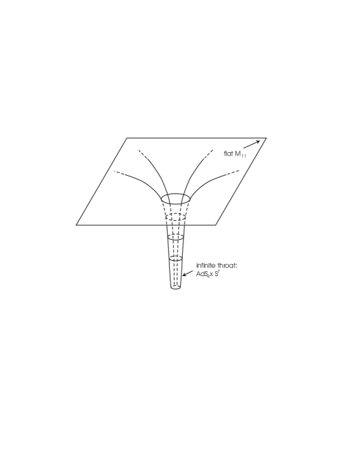
Figure 5.1: The M2-brane interpolates between $\mathcal{M}_{11}:=(\mathbb{R}^{11},\eta)$ and $AdS_{4}\times S^{7}$.

Another interesting aspect of the $M2$-brane solution is its interpolating character. It is obvious, that its limit for $r\rightarrow\infty$ is eleven-dimensional Minkowski space, provided $ds_{7}^{2}$ is the standard metric on the seven-sphere $S^{7}$. In that case the metric tends to $AdS_{4}\times S^{7}$ for $r\rightarrow 0$. So the membrane interpolates between two different vacua as is shown in figure 5.1. If $X$ is not the seven-sphere we still have the limit $AdS_{4}\times X$ for $r\rightarrow 0$, but for $r\rightarrow\infty$ we no longer obtain Minkowski space. What we get is $\mathcal{M}_{3}\times C(X)$, where $C(X)$ is the cone on $X$ and $\mathcal{M}_{3}$ is three-dimensional Minkowski space. These spaces will be analyzed in more detail below.
Recently a new type of solution was found [30] in which a self-dual harmonic four-form was added to the $G$-flux of (5.38). These kinds of solutions no longer have singularities. A variety of solutions of intersecting or wrapped M-branes can be found in the literature.

Next to the solutions we studied so far there is also the so called $pp$-wave solution [59] which has found renewed interest recently.

5.2 Supersymmetry in M-Theory - the Arisal of $G_{2}$

After having discussed several solutions of the equations of motion we now want to study whether these vacua preserve supersymmetry.

Definition 5.2
A vacuum $(M,\langle g\rangle,\langle C\rangle,\langle\psi\rangle)$ is said to be supersymmetric if it satisfies

$$\delta e_{\ \ M}^{A} := -{1\over 2}\bar{\eta}\Gamma^{A}\psi_{M}=0,$$

$$\delta C_{MNP} := -{3\over 2}\bar{\eta}\Gamma_{[MN}\psi_{P]}=0,$$ (5.39)

$$\delta\psi_{M} := \widetilde{\nabla}^{S}_{M}(\hat{\omega})\eta=0,$$

where the variations have to be calculated at the point $e^{A}_{\ \ M}=\langle e^{A}_{\ \ M}\rangle,\ C_{MNP}=\langle C_{MNP}\rangle,\ \psi_{M}=\langle\psi_{M}\rangle$. All the vacua we are going to study have vanishing fermionic background, $\langle\psi_{M}\rangle=0$, so the first two equations are trivially satisfied and the last one reduces to

$$\widetilde{\nabla}^{S}_{M}(\omega)\eta=0,$$ (5.40)

evaluated at $C_{MNP}=\langle C_{MNP}\rangle$, $e^{A}_{\ \ M}=\langle e^{A}_{\ \ M}\rangle$ and $\psi_{M}=0$. We see that $e^{A}_{\ \ M}$ and $C_{MNP}$ are automatically invariant and we find that the vacuum is supersymmetric if and only if there exists a spinor $\eta$ s.t. $\forall M$

$$\nabla^{S}_{M}\eta-{1\over 288}\left(\Gamma_{M}^{\ \ PQRS}-8\delta_{M}^{P}\Gamma^{QRS}\right)G_{PQRS}\eta=0.$$ (5.41)

We will now analyze the implications of this equation for the vacua we studied above. See [21], [36] and [38] for a discussion of some of the topics covered in this section.

5.2.1 Ricci-flat Solutions and $G_{2}$

In this section we study the amount of supersymmetry that is preserved by Ricci-flat solutions. As we saw above, these are Riemannian products of Minkowski space and a seven-dimensional space that is Ricci-flat. $G$-flux and the fermionic background are taken to vanish.
Given these conditions of the vacuum we get a further simplification of (5.41), which now reads

$$\nabla^{S}\eta=0.$$ (5.42)

To be able to determine the number of supersymmetries in a given vacuum we need to comment on supersymmetry in various dimensions. A supersymmetric theory in $d$ dimensions is one in which the Poincaré algebra is extended to a superalgebra by adding spinorial generators $Q^{I}_{\alpha}$. $I$ is a label with $I\in\{1,\ldots,\mathcal{N}\}$, $\mathcal{N}\in\mathbb{N}$ and $\mathcal{N}$ gives the number of supersymmetries of the theory. For $\mathcal{N}=1$ we speak of unextended supersymmetry, otherwise supersymmetry is said to be extended. The index $\alpha$ runs over the spin components of the spinor $Q^{I}$, but this means that the range of $\alpha$ depends on the dimension $d$, because the number of components of a spinor depends on $d$ (see appendix B). At the moment we are particularly interested in the case $d=11$ where a spinor has 32 components and the case $d=4$ with 4 component spinors. Suppose we start from a theory with $\mathcal{N}=1$ in eleven dimensions and we compactify to four dimensions. If the compactification is done in a way that all the 32 generators are generators of supersymmetry in the four-dimensional theory we obtain $\mathcal{N}=8$. So we conclude that starting from $\mathcal{N}=1$ in $d=11$ we can have $0\leq\mathcal{N}\leq 8$ in $d=4$. We note in passing that there are no consistent four-dimensional theories with $\mathcal{N}>8$ as this would lead to particles of spin bigger than two for which no consistent field theories are known. Similarly, in eleven dimensions $\mathcal{N}=1$ is the only possibility.
Let us be more precise. A supersymmetric vacuum in eleven dimensions is one that admits 32 linearly independent solutions of equation (5.42) corresponding to 32 generators of supersymmetry. After compactification the original Poincaré group $P(10,1)$ is broken to $P(3,1)\times P(7)$. The ${\bf 32}$ of $SO(10,1)$ decomposes as ${\bf 32}={\bf 4}\otimes{\bf 8}$, thus, for a spinor in the compactified theory we have

$$\eta(x,y)=\epsilon(x)\otimes\theta(y),$$ (5.43)

with $\epsilon$ a spinor in four and $\theta$ a spinor in seven dimensions. The $\Gamma$-matrices can be rewritten as
$\displaystyle\Gamma^{a}$ $\displaystyle=$ $\displaystyle\gamma^{a}\otimes\leavevmode\hbox{\small 1\kern-3.8pt\normalsize 1},$ $\displaystyle\Gamma^{m}$ $\displaystyle=$ $\displaystyle\gamma_{5}\otimes\gamma^{m},$ with $\{\gamma^{m}\}$ the generators of a Clifford algebra in seven dimensions. This leads to a nice decomposition of $\nabla^{S}=\nabla_{M}^{S}dz^{M}$,

$$\nabla^{S} = \nabla_{\mu}^{S}dx^{\mu}+\nabla^{S}_{m}dy^{m}$$ (5.45)

$$= (\partial_{\mu}+{1\over 4}\omega_{\mu AB}\Gamma^{AB})dx^{\mu}+(\partial_{m}+{1\over 4}\omega_{mAB}\Gamma^{AB})dy^{m}$$

$$= (\partial_{\mu}+{1\over 4}\omega_{\mu ab}\Gamma^{ab})dx^{\mu}+(\partial_{m}+{1\over 4}\omega_{m\hat{n}\hat{p}}\Gamma^{\hat{n}\hat{p}})dy^{m}$$

$$= (\partial_{\mu}+{1\over 4}\omega_{\mu ab}\gamma^{ab}\otimes\leavevmode\hbox{\small 1\kern-3.8pt\normalsize 1})dx^{\mu}+(\partial_{m}+{1\over 4}\omega_{m\hat{n}\hat{p}}\leavevmode\hbox{\small 1\kern-3.8pt\normalsize 1}\otimes\gamma^{\hat{n}\hat{p}})dy^{m}$$

$$= \nabla^{S}_{4}\otimes\leavevmode\hbox{\small 1\kern-3.8pt\normalsize 1}+\leavevmode\hbox{\small 1\kern-3.8pt\normalsize 1}\otimes\nabla_{7}^{S}.$$

Here we used the fact that our vacuum is a Riemannian product, and thus the connection coefficients with mixed indices, as $\omega_{m\hat{n}a}$, vanish. But then (5.42) reads

$$(\nabla^{S}_{4}\otimes\leavevmode\hbox{\small 1\kern-3.8pt\normalsize 1}+\leavevmode\hbox{\small 1\kern-3.8pt\normalsize 1}\otimes\nabla_{7}^{S})\epsilon(x)\otimes\theta(y)=\nabla^{S}_{4}\epsilon(x)\otimes\theta(y)+\epsilon(x)\otimes\nabla_{7}^{S}\theta(y)=0.$$ (5.46)

We are looking for the number of linearly independent solutions of this equations for a given vacuum. Any maximally symmetric space admits the maximum number of covariantly constant spinors, in particular, on Minkowski space we can find a basis of four constant spinors $\epsilon^{i}$. The condition we are left with is

$$\nabla^{S}_{7}\theta(y)=0.$$ (5.47)

Thus, the number of solutions of (5.42) is four times the number of covariantly constant spinors on the compact seven manifold. This in turn implies that the number of supersymmetries in four dimensions is given by the number of covariantly constant spinors on the seven-manifold.

After these comments it is easy to determine the amount of supersymmetry preserved by various vacua. The first vacuum we found was eleven-dimensional Minkowski space. Obviously, in this case we can find 32 covariantly constant spinors, we have a vacuum with $\mathcal{N}=1$ supersymmetry. The spaces which are more interesting are $\mathbb{R}^{4}\times T^{7}$ and $\mathbb{R}^{4}\times T^{3}\times K3$. $T^{7}$ is flat, hence, we expect to find 8 solutions of (5.47). This gives the maximal $\mathcal{N}=8$ supersymmetry in four dimensions. The situation gets more interesting for $\mathbb{R}^{4}\times T^{3}\times K3$. The reason is that the K3 surface has the reduced holonomy $SU(2)$, and from theorem 2.23 we read off that we are left with only two covariantly constant spinors. We have the decomposition ${\bf 32}={\bf 4}\otimes{\bf 2}\otimes{\bf 4}$ and as we get two solutions for $T^{3}$ we are left with sixteen solutions altogether, and thus $\mathcal{N}=4$ supersymmetry.

Our goal is to find a vacuum of M-theory which is a Riemannian product of Minkowski space and a compact seven-manifold, s.t. the effective field theory in four dimensions contains the field content of the standard model with $\mathcal{N}=1$ supersymmetry. After the discussions of this chapter it is easy to derive the consequences of the latter condition. $\mathcal{N}=1$ supersymmetry means that the compact space has exactly one covariantly constant spinor. Referring once again to theorem 2.23 we conclude that the holonomy group of the compact seven-dimensional space has to be $G_{2}$. These spaces are possible vacua because they are automatically Ricci-flat. So to find realistic field theories we should concentrate on compactifications on $G_{2}$-manifolds.
Before we proceed we want to understand the relation between a covariantly constant spinor and $G_{2}$ holonomy from a more physical point of view. It is clear that $\nabla^{S}_{7}\theta=0$ implies $R_{mn\hat{p}\hat{q}}\Gamma^{\hat{p}\hat{q}}\theta=0$. But $R_{mn\hat{p}\hat{q}}\Gamma^{\hat{p}\hat{q}}$ are the generators of the holonomy group on $M_{7}$. So we deduce $Hol(M_{7})\theta=\theta$ for exactly one spinor $\theta$. Using a suitable basis this spinor can be written as $\theta=(0,\ldots,0,1)^{\tau}$ and $Hol(M_{7})$ is the subgroup of $SO(7)$ which fixes this spinor, i.e. we must have ${\bf 8}\rightarrow{\bf 7}\oplus{\bf 1}$ under $Hol(M_{7})\subset SO(7)$. But this is true only for $Hol(M_{7})=G_{2}$.

Yet, we also need to mention at this point that compactification on $G_{2}$-manifolds is not the only possible method to obtain $\mathcal{N}=1$ supersymmetry from M-theory. The reason is that the requirements of theorem 2.23 are rather strong. In particular, we want the metric to be irreducible. This basically excludes the Riemannian product of two spaces. If we allow for manifolds $M_{7}$ which are Riemannian products a number of other interesting solutions with the right amount of supersymmetry exists. We mentioned above that the compactification of M-theory on $S^{1}$ and on $S^{1}/\mathbb{Z}_{2}$ gives the strong coupling limit of type IIA and $E_{8}\times E_{8}$ heterotic string theory. But it is well known [29] that the compactification of the heterotic string on Calabi-Yau three-folds, three-dimensional complex Ricci-flat manifolds with holonomy $SU(3)$, leads to $\mathcal{N}=1$ supersymmetry, as well. In fact the analysis of this case is very similar to what we did for M-theory in this chapter. Similarly, compactifying the IIA theory on a Calabi-Yau three-fold leads to $\mathcal{N}=2$ in four dimensions. We conclude that the desired amount of supersymmetry can be obtained from both compactifications of M-theory on $G_{2}$-manifolds as well as on $CY_{3}\times S^{1}/\mathbb{Z}_{2}$.

So far we only considered Ricci-flat solutions, which have to satisfy very restrictive conditions. However, it was shown in [28] that any supersymmetric compactification of eleven-dimensional supergravity to $(\mathbb{R}^{4}\times M_{7},\eta\times g)$, with $(\mathbb{R}^{4},\eta)$ Minkowski space and $(M_{7},g)$ arbitrary but compact, leads to vanishing G-flux, $\langle C\rangle=0$, and a Ricci-flat compact space $\mathcal{R}_{mn}=0$.
If one relaxes the constraint of compactifications to Minkowski space there are other supersymmetric vacua, as we will see in the next section.

5.2.2 The Freund-Rubin Solutions and Weak $G_{2}$

Next we want to analyze the consequences of (5.41) for the Freund-Rubin solutions. Remember that we have $\langle G_{mnpq}\rangle=0$ and $\langle G_{\mu\nu\rho\sigma}\rangle=f\epsilon_{\mu\nu\rho\sigma}$ in this case. With

$$\gamma_{5}:=-i\gamma^{\hat{0}}\gamma^{\hat{1}}\gamma^{\hat{2}}\gamma^{\hat{3}}=-{i\over 4!}\gamma^{\mu}\gamma^{\nu}\gamma^{\rho}\gamma^{\sigma}\epsilon_{\mu\nu\rho\sigma}$$ (5.48)

and

$$\epsilon_{\mu\nu\rho\sigma}\gamma^{\nu}\gamma^{\rho}\gamma^{\sigma}=6i\gamma_{\mu}\gamma_{5}$$ (5.49)

we get
$\displaystyle\nabla^{S}_{\mu}\eta$ $\displaystyle=$ $\displaystyle-{if\over 6}(\gamma_{\mu}\gamma_{5}\otimes\leavevmode\hbox{\small 1\kern-3.8pt\normalsize 1})\eta,$ $\displaystyle\nabla^{S}_{m}\eta$ $\displaystyle=$ $\displaystyle{if\over 12}(\leavevmode\hbox{\small 1\kern-3.8pt\normalsize 1}\otimes\gamma_{m})\eta,$ where we used the same decomposition of spinors and $\Gamma$-matrices as in the Ricci-flat case. Again we have the decomposition ${\bf 32}={\bf 4}\otimes{\bf 8}$ and hence

$$\eta(x,y)=\epsilon(x)\otimes\theta(y).$$ (5.51)

Then (LABEL:Deta) reduce to

$$\nabla^{S}_{\mu}\epsilon = -{if\over 6}\gamma_{\mu}\gamma_{5}\epsilon,$$ (5.52)

$$\nabla^{S}_{m}\theta = {if\over 12}\gamma_{m}\theta.$$ (5.53)

From standard supergravity theory in four dimensions [34] one can show that on $AdS$ there are always four spinors satisfying (5.52). Therefore, the number of spinors $\eta$, satisfying (LABEL:Deta) is four times the number of spinors $\theta$ which are solutions of (5.53). But this implies that the number of supersymmetry being conserved is given by the number of solutions of (5.53).

Let us pause for a moment and check whether the condition of a supersymmetric vacuum is consistent. To do so we calculate

$$\ [\nabla^{S}_{\mu},\nabla^{S}_{\nu}]\epsilon = -{f^{2}\over 36}(\gamma_{\mu}\gamma_{\nu}-\gamma_{\nu}\gamma_{\mu})\epsilon,$$ (5.54)

$$\ [\nabla^{S}_{m},\nabla^{S}_{n}]\theta = {f^{2}\over 144}(\gamma_{m}\gamma_{n}-\gamma_{n}\gamma_{m})\theta,$$ (5.55)

and using (D.13) we obtain

$$\mathcal{R}_{\mu\nu} = -{1\over 3}f^{2}g_{\mu\nu},$$ (5.56)

$$\mathcal{R}_{mn} = {1\over 6}f^{2}g_{mn}.$$ (5.57)

But this is exactly (5.12) and (5.13), thus it is consistent to look for supersymmetric Freund-Rubin type solutions.

So to find Freund-Rubin solutions with $\mathcal{N}=k$ supersymmetry we need to find compact seven-dimensional Einstein spaces with positive curvature and exactly $k$ Killing spinors. One possible space is the seven-sphere which admits eight Killing spinors, leading to maximal supersymmetry in four dimensions.
Another interesting example was found in [13]. There the compact space has the topology of a sphere, but the metric has been “squashed” and it no longer is the standard metric. In fact, it admits exactly one Killing spinor, leading to $\mathcal{N}=1$ supersymmetry. Here we can take up a comment from chapter 2, as this sphere actually has weak $G_{2}$ holonomy. The reader is referred to the literature for further details.

In fact, the Freund-Rubin ansatz is not the most general ansatz to find solutions which are a Riemannian product of a maximally symmetric space in four dimensions and a compact seven-manifold. In [43] a solution with $\langle G_{mnpq}\rangle\neq 0$ was found. However, it was shown in [33] and [44] that it breaks all supersymmetry. This is actually the case for all solutions with $\langle G_{mnpq}\rangle\neq 0$, therefore they are not interesting for our purposes.

5.2.3 M2-branes and Supersymmetry

We now want to turn to the question of how much supersymmetry is conserved in the case of the M2-brane solution. We saw already that the amount of supersymmetry which is conserved by a given vacuum depends on the metric on this vacuum. Therefore, it is natural to expect that preserved supersymmetry depends on the metric of the Ricci-flat compact seven-manifold $X$, which has not been specified so far. This will indeed turn out to be true.
As always the fermionic background vanishes and we need to analyze once again the consequences of (5.41). Because of the specific structure of the M2-brane with a (2+1)-dimensional Minkowski space, a radial coordinate $x^{3}:=r$ and a compact seven-manifold $X$ we look at the decomposition ${\bf 32}={\bf 4}\otimes{\bf 8}={\bf 2}\otimes{\bf 2}\otimes{\bf 8}$. We write our spinors as

$$\eta=\epsilon\otimes\theta,$$ (5.58)

with a four component spinor $\epsilon$ on the (1+2+1)-dimensional space and an eight component spinor $\theta$ on the seven-manifold $X$. However, we decompose the $\Gamma$-matrices as

$$\Gamma^{\hat{a}} = \gamma^{\hat{a}}\otimes\sigma_{3}\otimes\leavevmode\hbox{\small 1\kern-3.8pt\normalsize 1},$$

$$\Gamma^{\hat{3}} = \leavevmode\hbox{\small 1\kern-3.8pt\normalsize 1}\otimes\sigma_{1}\otimes\leavevmode\hbox{\small 1\kern-3.8pt\normalsize 1},$$ (5.59)

$$\Gamma^{\hat{m}} = \leavevmode\hbox{\small 1\kern-3.8pt\normalsize 1}\otimes\sigma_{2}\otimes\gamma^{\hat{m}}.$$

Before we proceed any further we collect some useful relations. From (LABEL:omegas) we can read off that the only non-vanishing components of the spin connection are

$$\omega_{\hat{a}\ \hat{3}}^{\ \hat{b}} = -{1\over 3}H^{\prime}H^{-{7\over 6}}\delta_{\hat{a}}^{\hat{b}},$$

$$\omega_{\hat{m}\ \hat{n}}^{\ \hat{3}} = -\left({H^{\prime}\over 6H}+{1\over r}\right)H^{-{1\over 6}}\delta_{\hat{m}\hat{n}},$$ (5.60)

$$\omega_{\hat{n}\ \hat{q}}^{\ \hat{p}} = \widetilde{\omega}_{\hat{n}\ \hat{q}}^{\ \hat{p}}.$$

Furthermore, from (LABEL:vielbeins) we get

$$e_{\hat{a}}^{b} = H^{1\over 3}\delta^{b}_{\hat{a}},$$

$$e_{\hat{3}}^{\ 3} = H^{-{1\over 6}},$$ (5.61)

$$e_{\hat{n}}^{\ m} = {1\over r}H^{-{1\over 6}}\widetilde{e}_{\hat{n}}^{\ m}.$$

$\Gamma$-matrix conventions on the three-dimensional Minkowski space are such that $\gamma^{\hat{0}}\gamma^{\hat{1}}\gamma^{\hat{2}}=-\leavevmode\hbox{\small 1\kern-3.8pt\normalsize 1}$. Then, the substitution of the M2-brane solution into (5.41) gives [38]

$$0 = \delta_{\hat{a}}^{b}H^{{1\over 3}}\partial_{b}\eta+{1\over 6}H^{\prime}H^{-{7\over 6}}\gamma_{\hat{a}}\otimes\sigma_{1}(\sigma_{3}-\leavevmode\hbox{\small 1\kern-3.8pt\normalsize 1})\otimes\leavevmode\hbox{\small 1\kern-3.8pt\normalsize 1}\eta,$$

$$0 = H^{-{1\over 6}}\partial_{r}\eta+{1\over 6}H^{\prime}H^{-{7\over 6}}\leavevmode\hbox{\small 1\kern-3.8pt\normalsize 1}\otimes\sigma_{3}\otimes\leavevmode\hbox{\small 1\kern-3.8pt\normalsize 1}\eta,$$ (5.62)

$$0 = {1\over r}H^{-{1\over 6}}\left(\widetilde{e}_{\hat{m}}^{\ \ n}\leavevmode\hbox{\small 1\kern-3.8pt\normalsize 1}\otimes\leavevmode\hbox{\small 1\kern-3.8pt\normalsize 1}\otimes\nabla_{n}^{S}\eta-{i\over 2}\leavevmode\hbox{\small 1\kern-3.8pt\normalsize 1}\otimes\sigma_{3}\otimes\gamma_{\hat{m}}\eta\right)-{i\over 12}H^{\prime}H^{-{7\over 6}}\leavevmode\hbox{\small 1\kern-3.8pt\normalsize 1}\otimes(\sigma_{3}-\leavevmode\hbox{\small 1\kern-3.8pt\normalsize 1})\otimes\gamma_{\hat{m}}\eta.$$

Again we are looking for the number of solutions $\eta$ of this set of equations. The problem simplifies if we recall its symmetries. We have a $P(2,1)$ symmetry on the three-dimensional Minkowski space and a radial coordinate which can be viewed as parameterizing seven-manifolds $X$. The most general spinor that is invariant under the symmetries of this setup has the form

$$\eta=F(r)\epsilon_{0}\otimes\theta,$$ (5.63)

with $\epsilon_{0}$ a constant spinor. If we plug this ansatz into (5.62) we get conditions for our spinor,

$$F^{\prime}=-{H^{\prime}\over 6H}F,$$ (5.64)

$$\leavevmode\hbox{\small 1\kern-3.8pt\normalsize 1}\otimes\sigma_{3}\epsilon_{0}=\epsilon_{0},$$ (5.65)

$$\nabla^{S}_{\hat{m}}\theta-{i\over 2}\gamma_{\hat{m}}\theta=0.$$ (5.66)

The first equation can easily be integrated and gives $F=H^{-{1\over 6}}$. The second equation is more interesting as it is satisfied by only two of the four constant spinors on the (1+2+1)-dimensional space. The last equation tells us that $\theta$ has to be a Killing spinor on the seven-dimensional space $X$. This is all very nice. We conclude that the number of solutions of (5.41) is two times the number of Killing spinors on $X$. For example in the case of the seven-sphere, $X=S^{7}$, we have eight Killing spinors and hence sixteen generators of supersymmetry. We see that in this case an M2-brane breaks half of the supersymmetry. Certainly we can find a solution which breaks supersymmetry completely. All one has to do is to look for a compact Ricci-flat seven-manifold with $\mathcal{R}_{mn}=6\delta_{mn}$ that does not admit Killing spinors. But there are also interesting spaces in between these two cases. In particular let us consider a space with weak $G_{2}$ holonomy. We know that these spaces admit exactly one Killing spinor and that they are Einstein spaces with positive scalar curvature. In that case only two supersymmetric generators remain unbroken, we speak of a weak $G_{2}$-brane.

5.3 Kaluza-Klein Compactification on Smooth $G_{2}$-Manifolds

The analysis of the structure of $G_{2}$-manifolds showed that M-theory on $(\mathcal{M}_{4}\times X,\eta\times g)$ with $(X,g)$ a $G_{2}$-manifold leads to an effective $\mathcal{N}=1$ supergravity theory in four dimensions. In this section we want to analyze the field content that arises from Kaluza-Klein compactification on smooth $G_{2}$-manifolds. This field content was determined in [70], the compactification procedure is reviewed in [3].
We start from supergravity (LABEL:SUGRAaction) on the Riemannian product $(\mathcal{M}_{4}\times X,\eta\times g)$. Together with $\langle\psi_{M}\rangle=\langle C\rangle=0$ this is a possible vacuum of eleven-dimensional supergravity. We assume that $X$ is large compared to the Planck length in order for supergravity to be valid and small compared to macroscopic scales. In particular, it is supposed to be so small that massive Kaluza-Klein states cannot be observed.

Proposition 5.3
The low energy effective theory of M-theory on $(\mathcal{M}_{4}\times X,\eta\times g)$ with $(X,g)$ a smooth $G_{2}$-manifold is an $\mathcal{N}=1$ supergravity theory coupled to $b^{2}(X)$ Abelian vector multiplets and $b^{3}(X)$ massless neutral chiral multiplets.

In order to show this we proceed according to the recipe given in section 3.3. Consider small fluctuations around the vacuum,

$$g_{MN}(x,y) = \langle g_{MN}(x,y)\rangle+\delta g_{MN}(x,y),$$ (5.67)

$$C(x,y) = \langle C(x,y)\rangle+\delta C(x,y)=\delta C(x,y),$$ (5.68)

$$\psi_{M}(x,y) = \langle\psi_{M}(x,y)\rangle+\delta\psi_{M}(x,y)=\delta\psi_{M}(x,y).$$ (5.69)

Next we need to substitute these fluctuations into the field equations, keeping only linear terms.

Kaluza-Klein expansion of the $C$-field

After substitution of (5.68) the equation for the C-field reads

$$d*G=0.$$ (5.70)

If we impose the gauge condition $d*C=0$ we get

$$\Delta_{11}C=0.$$ (5.71)

We split $\Delta_{11}=\Delta_{4}+\Delta_{7}$,

$$\Delta_{4}C+\Delta_{7}C=0,$$ (5.72)

to see that possible mass terms for four dimensional fields might arise from $\Delta_{7}C$, which is identified with the mass operator of equation (3.150).

Let $\{\Omega^{i}\}\subset\Lambda^{3}T^{*}X$ be the set of three-forms, s.t.

$$\Delta_{7}\Omega^{i}=\lambda^{i}_{(3)}\Omega^{i},$$ (5.73)

$\{\omega^{j}\}\subset\Lambda^{2}T^{*}X$ be the set of two-forms, s.t.

$$\Delta_{7}\omega^{j}=\lambda^{j}_{(2)}\omega^{j},$$ (5.74)

$\{a^{k}\}\subset\Lambda^{1}T^{*}X$ be the set of one-forms, s.t.

$$\Delta_{7}a^{k}=\lambda^{k}_{(1)}a^{k},$$ (5.75)

and let $\{g^{l}\}\subset\Lambda^{0}T^{*}X$ be the set of eigenfunctions, s.t.

$$\Delta_{7}g^{l}=\lambda^{l}_{(0)}g^{l}.$$ (5.76)

Then we have the general expression

$$C(x,y) = \sum_{i}p^{i}(x)\wedge\Omega^{i}(y)+\sum_{j}A^{j}(x)\wedge\omega^{j}(y)$$ (5.77)

$$+\sum_{k}B^{k}(x)\wedge a^{k}(y)+\sum_{l}H^{l}(x)\wedge g^{l}(y).$$

This can be rewritten as

$$C(x,y) = \sum_{i=1}^{b^{3}(X)}p^{i}(x)\wedge\Omega^{i}(y)+\sum_{j=1}^{b^{2}(X)}A^{j}(x)\wedge\omega^{j}(y)$$ (5.78)

$$+\sum_{k^{1}}^{b^{1}(X)}B^{k}(x)\wedge a^{k}(y)+\sum_{l=1}^{b^{0}(X)}H^{l}(x)\wedge g^{l}(y)+\ldots\mbox{(massive)},$$

where from now on $\Omega^{i},\ \omega^{j},\ a^{k}$ and $g^{l}$ are taken to be harmonic forms on $X$. Given the Betti numbers of a $G_{2}$-manifold this simplifies to

$$C(x,y)=\sum_{i=1}^{b^{3}(X)}p^{i}(x)\wedge\Omega^{i}(y)+\sum_{j=1}^{b^{2}(X)}A^{j}(x)\wedge\omega^{j}(y)+H(x)+\ldots\ \mbox{(massive)}.$$ (5.79)

We see that we obtain $b^{2}(X)$ Abelian gauge fields and $b^{3}(X)$ pseudo-scalar fields from compactifications of the $C$-field. Note that a necessary requirement was that $\langle G\rangle=\langle\psi_{M}\rangle=0$, so this kind of expansion of the $C$-field is only valid for vacua with vanishing $G$-flux.

Kaluza-Klein expansion of the metric

Compactifying the $C$-field gave us $b^{3}(X)$ pseudo-scalars in four dimensions. In eleven dimensions the bosonic superpartner of $C$ is $g$, so we should expect that superpartners of the pseudo-scalars in four dimensions can be obtained from the metric, which therefore should give another $b^{3}(X)$ scalars. To see this explicitly we substitute the fluctuations into the Einstein equation. As the energy momentum tensor is quadratic in the fluctuations we are left with the condition of Ricci-flatness,

$$\mathcal{R}_{MN}=0,$$ (5.80)

where $\mathcal{R}_{MN}$ is evaluated using the full metric of (5.67). Suppose furthermore that $\delta g_{\mu m}(x,y)=0$, which (together with the Riemannian product structure of our eleven-dimensional manifold) implies that Christoffel symbols with mixed components vanish trivially. Then (5.80) reduces to $\mathcal{R}_{\mu\nu}=\mathcal{R}_{mn}=0$. Substitution of $g_{mn}(x,y)=\langle g_{mn}(x,y)\rangle+\delta g_{mn}(x,y)$ leads to the Lichnerowicz equation for $\delta g_{mn}$,

$$\Delta_{L}\delta g_{mn}:=-\Delta_{11}\delta g_{mn}-2R_{mpnq}\delta g^{pq}+2\mathcal{R}^{\ \ p}_{(m}\delta g_{n)p}=0,$$ (5.81)

where now $R_{mpnq}$ and $\mathcal{R}_{pm}$ are calculated from $\langle g_{mn}\rangle$. Again we write $\Delta_{11}=\Delta_{4}+\Delta_{7}$ and obtain

$$\Delta_{4}\delta g_{mn}+\Delta_{7}\delta g_{mn}+2R_{mpnq}\delta g^{pq}-2\mathcal{R}_{(m}^{\ \ p}\delta g_{n)p}=0.$$ (5.82)

Next we make the Kaluza-Klein ansatz

$$\delta g_{mn}(x,y)=\sum_{i}s^{i}(x)h^{i}_{mn}(y),$$ (5.83)

where $h^{i}_{mn}$ are eigenfunctions of the Lichnerowicz operator

$$\Delta_{L}h^{i}_{mn}(y)=\lambda^{i}h^{i}_{mn}(y).$$ (5.84)

Then we are left with

$$0 = \left(\Delta_{4}s^{i}(x)\right)h^{i}_{mn}(y)-s^{i}(x)\Delta_{L}h^{i}_{mn}(y)$$ (5.85)

$$= \left(\Delta_{4}s^{i}(x)-\lambda^{i}s^{i}(x)\right)h^{i}_{mn}(y).$$

We conclude that massless scalar fields in four dimensions are given by the zero modes of the Lichnerowicz operator. It remains to determine the number of zero modes. To do so we define the three-form $\omega$ s.t.

$$\omega_{mnp}:=\varphi_{q[mn}h^{\ \ q}_{p]},$$ (5.86)

where $\varphi$ is the $G_{2}$-invariant three-form on $X$. It can be shown [3] that $h$ is a zero mode of the Lichnerowicz operator if and only if $\omega$ is harmonic,

$$\Delta_{L}h=0\ \ \ \Leftrightarrow\ \ \ \Delta\omega=0.$$ (5.87)

To prove this we need to note that

$$\varphi_{q[mn}R_{p]k\ l}^{\ \ \ q}h^{kl}=0,$$ (5.88)

which gives

$$\Delta\omega_{mnp}=-\varphi_{q[mn}\Delta_{L}h_{p]}^{\ \ q}$$ (5.89)

and thus the desired result. We conclude that there are $b^{3}(X)$ scalars in the four dimensional theory coming from the metric, as expected.
In fact, this could have been anticipated from the general rule that if there is a $k$-dimensional family of $G_{2}$-holonomy metrics on $X$, i.e. if the moduli space of these metrics has dimension $k$, then there will be correspondingly $k$ massless scalars in four dimensions. From proposition 2.34 we know that the moduli space of $G_{2}$ metrics on $X$ is a manifold of dimension $b^{3}(X)$.
Now, the scalars coming from the metric combine with those coming from the $C$-field to give $b^{3}(X)$ complex massless scalars $\Phi^{i}(x):=s^{i}+ip^{i}$ which are the lowest components of massless chiral superfields in four dimensions. These scalar fields can be rewritten in a very nice form by means of a basis $\alpha_{i}$ for the third homology group of $X$, $H_{3}(X,\mathbb{R})$. The basis is chosen s.t.

$$\int_{\alpha_{j}}\Omega^{i}=\delta^{ij}.$$ (5.90)

Next we note that a fluctuation of the metric can be rewritten by means of the three-form $\varphi$ characterizing a $G_{2}$-manifold,

$$\varphi^{\prime}=\varphi+\delta\varphi=\varphi+\sum_{i}s^{i}(x)\Omega^{i}(y).$$ (5.91)

This gives

$$\Phi^{i}=\int_{\alpha_{i}}\left(\varphi^{\prime}+iC\right).$$ (5.92)

It remains to consider the fluctuations of the metric on four-dimensional Minkowski space. As above the substitution of $g_{\mu\nu}(x,y)=\langle g_{\mu\nu}(x,y)\rangle+\delta g_{\mu\nu}(x,y)$ into $\mathcal{R}_{\mu\nu}(g_{\rho\sigma})$ leads to the Lichnerowicz equation for $\delta g_{\mu\nu}$. But on Minkowski space this equation simplifies to

$$\Delta_{11}\delta g_{\mu\nu}=0.$$ (5.93)

The Kaluza-Klein ansatz

$$\delta g_{\mu\nu}(x,y)=\sum_{i}h^{i}_{\mu\nu}(x)t^{i}(y),$$ (5.94)

with $t^{i}$ eigenfunctions of $\Delta_{7}$ gives

$$0 = \left(\Delta_{4}h^{i}_{\mu\nu}(x)\right)t^{i}(y)+h^{i}_{\mu\nu}(x)\Delta_{7}t^{i}(y)$$ (5.95)

$$= \left(\Delta_{4}h^{i}_{\mu\nu}(x)+\lambda^{i}h^{i}_{\mu\nu}(x)\right)t^{i}(y).$$

The massless particle corresponding to the zero modes of $\Delta_{7}$ is the four-dimensional graviton.

The isometry group of a compact $G_{2}$-manifold is trivial, as we will prove below. This implies that we do not get gauge fields from the Kaluza-Klein expansion of the metric.

We could perform a Kaluza-Klein expansion of the gravitino as well. However, this is not necessary, as we know from considerations in the last section that the effective four-dimensional theory has $\mathcal{N}=1$ supersymmetry. Hence, there will be superpartners to all the bosonic particles we considered so far. In particular, we will get the four-dimensional gravitino and hence supergravity. But this supergravity theory is coupled to a gauge theory with $b^{2}(X)$ Abelian vectors multiplets and $b^{3}(X)$ neutral chiral multiplets. This means that the total number of fermions is $b^{2}(X)+b^{3}(X)$ together with the gravitino.

Unfortunately the theory we obtained is not very interesting. Neither did we find non-Abelian gauge groups which are a crucial ingredient of the standard model, nor do we have charged chiral fermions in our effective theory. Obviously the fermionic superpartners of the Abelian gauge fields are neutral. The effective action contains no term which couples the chiral multiplets to the Abelian gauge fields, so we conclude that their charges vanish as well. This means that we have to work harder to get a realistic theory from compactifications on $G_{2}$-manifolds. Note on the other hand that the theory is automatically free of local gauge anomalies, as the fermions cannot couple to the gauge fields.

The isometry group of a manifold with $G_{2}$-holonomy

In chapter 3 we discussed that non-Abelian gauge groups are generated by the isometry group of the compact manifold. To prove the statement that our Kaluza-Klein compactification does not lead to non-Abelian gauge theories we must show that the isometry group of a $G_{2}$-manifold is trivial.

Proposition 5.4
A compact manifold $X$ with holonomy group $G_{2}$ does not have continuous symmetries.

Continuous symmetries are generated by Killing vectors, so it is sufficient to show, that there are no Killing vectors on $X$. A Killing vector $V$ satisfies

$$\nabla_{m}V_{n}+\nabla_{n}V_{m}=0.$$ (5.96)

Multiplying by $g^{mn}$ we get $\nabla^{m}V_{m}=0$. Furthermore

$$0=\nabla^{m}\nabla_{m}V_{n}+\nabla^{m}\nabla_{n}V_{m}.$$ (5.97)

But using (D.10)

$$\nabla^{m}\nabla_{n}V_{m}=\nabla_{n}\nabla^{m}V_{m}+[\nabla^{m},\nabla_{n}]V_{m}=R^{m}_{\ nmp}V^{p}=\mathcal{R}_{np}V^{p}=0,$$ (5.98)

as $X$ is Ricci flat. We are left with

$$\nabla^{m}\nabla_{m}V_{n}=0.$$ (5.99)

This implies for compact manifolds $X$

$$0=\int_{X}V^{n}\nabla^{m}\nabla_{m}V_{n}=-\int_{X}(\nabla^{m}V^{n})(\nabla_{m}V_{n}),$$ (5.100)

therefore, the Killing vector must be covariantly constant,

$$\nabla_{m}V_{n}=0.$$ (5.101)

Thus we proved the following Lemma.

Lemma 5.5
A Killing vector on a Ricci-flat compact manifold is covariantly constant.

But for $G_{2}\subset SO(7)$ we have ${\bf 7}\rightarrow{\bf 7}$, a vector always transforms in the fundamental representation of $G_{2}$. In particular, there is no singlet of the holonomy group, so covariantly constant vectors cannot exist on manifolds with holonomy $G_{2}$. Thus, there are no Killing vectors and the isometry group is trivial.

A final remark

It is interesting to compare our result to the effective theory obtained by compactifying the heterotic string on a Calabi-Yau manifold. In this case the effective theory is again an $\mathcal{N}=1$ supergravity theory in four dimensions. However, the two compactifications cannot be equivalent, as the compactification of the heterotic string leads to a chiral theory with non-abelian gauge fields. Some attempt have been made [70] to establish the equivalence of the two compactification schemes by compactifying the heterotic string on a Calabi-Yau manifold with zero Euler number, as this leads to non-chiral theories. If in addition the gauge group of the heterotic string can be broken to $U(1)^{16}$ the effective theory is $\mathcal{N}=1$ supergravity coupled to 16 $\mathcal{N}=1$ vector multiplets and $(h^{1,1}+h^{1,2}+1)$ $\mathcal{N}=1$ neutral chiral multiplets. The vanishing Euler number gives $h^{1,1}=h^{1,2}$. So the two compactification mechanisms lead to the same theory, provided $b^{2}(X)=16$ and $b^{3}(X)=2h^{1,1}+1$. This can be established for example for a Calabi-Yau manifold with $h^{1,1}=h^{1,2}=19$ and a $G_{2}$-manifold with $b^{2}(X)=16$ and $b^{3}(X)=39$. Remarkably, these manifolds exist [70], [61], [63].
The relation between the two compactification schemes will become much clearer when we will consider $G_{2}$-manifolds carrying singularities.

Chapter 6 M-theory Anomalies in the Presence of M-branes

So far we have seen that M2-branes and M5-branes are solutions of the equations of motions of eleven-dimensional supergravity. In fact, the action of those objects is known [6], [14], [19], and they can be coupled to the supergravity theory. This is similar to Maxwell’s theory where the action for electrons and magnetic monopoles can be coupled to the free photon field. However, we need to check whether this new theory is consistent, and in particular whether it is free of anomalies.

Five-branes in M-theory

The five-brane has support on a 5+1-dimensional submanifold $W^{6}$ of eleven-dimensional space-time $M_{11}$. Both $W^{6}$ and $M_{11}$ are taken to be oriented and spin. For this particular setup the notion of a normal bundle is useful.

Definition 6.1
Let $M$ be an $m$-dimensional submanifold of $\mathbb{R}^{m+k}$ and let $p\in M$. Then $T_{p}M\subset T_{p}\mathbb{R}^{m+k}\cong\mathbb{R}^{m+k}$. Define $N_{p}M\subset T_{p}\mathbb{R}^{m+k}$ to be the vector space which is normal to $T_{p}M$ in $T_{p}\mathbb{R}^{m+k}$, i.e. $u\cdot v=0$ $\forall u\in N_{p}M,\ \forall v\in T_{p}M$, with respect to the metric on $\mathbb{R}^{m+k}$. Then the normal bundle of $M$ is defined as $NM:=\cup_{p\in M}N_{p}M$.

$TM_{11}$ and $TW^{6}$ denote the tangent bundle of $M_{11}$ and $W^{6}$, respectively. If $TM_{11}|_{W^{6}}$ is the restriction of $TM_{11}$ on $W^{6}$ it can be written as a Whitney sum $TM_{11}|_{W^{6}}=TW^{6}\oplus NW^{6}$. Let $X^{M}(\xi^{\mu})$ be the embedding functions of $W^{6}$ into $M_{11}$, where $\mu,\nu,\ldots\in\{0,1,\ldots 5\}$ (with corresponding tangent space indices $a,b,\ldots$). This embedding breaks the original $SO(10,1)$ Lorentz symmetry to $SO(5,1)\times SO(5)$ and $GL(11,\mathbb{R})$ is broken to $GL(6,\mathbb{R})\times GL(5,\mathbb{R})$. $M_{11}$ carries a metric $g_{MN}$ which can be pulled back onto $W^{6}$. Then the components of the pullback $h:=X^{*}g$ read

$$h_{\mu\nu}(\xi^{\rho})={\partial X^{M}(\xi^{\rho})\over\partial\xi^{\mu}}{\partial X^{N}(\xi^{\rho})\over\partial\xi^{\nu}}g_{MN}(X(\xi^{\rho})).$$ (6.1)

From this metric we can construct the Levi-Civita connection and the curvature tensor on $W^{6}$, which we will denote $\widetilde{\Gamma}^{\rho}_{\mu\nu}$ and $\widetilde{R}_{\mu\nu\rho\sigma}$. It is useful to introduce coordinates on $M_{11}$, s.t. $W^{6}=\{p\in M_{11}|X^{6}=0,\ldots,X^{10}=0\}$ and $g_{\mu m}|_{{}_{W^{6}}}=\partial_{M}g_{\mu m}|_{{}_{W^{6}}}=0$, where $m,n,\ldots$ label the coordinates orthogonal to the brane. These coordinates reflect the broken symmetry of the system. Then, $g_{\mu\nu}(X(\xi))$ equals $h_{\mu\nu}(\xi)$ up to coordinate transformations on $W^{6}$. So in these coordinates we find $\Gamma_{\mu\nu}^{\rho}|_{{}_{W^{6}}}=\widetilde{\Gamma}^{\rho}_{\mu\nu}$. However, there is another interesting contribution of the eleven-dimensional connection. Consider

$$\Gamma_{\mu m}^{n}|_{{}_{W^{6}}}={1\over 2}g^{nM}(\partial_{\mu}g_{mM}+\partial_{m}g_{M\mu}-\partial_{M}g_{\mu m})|_{{}_{W^{6}}}={1\over 2}g^{nk}\partial_{\mu}g_{mk}|_{{}_{W^{6}}}.$$ (6.2)

We know, that $\omega^{A}_{MB}$ corresponding to $\Gamma_{MN}^{K}$ transforms as a connection under local Lorentz transformations, $\omega^{\prime}=g^{-1}(\omega+d)g$ with $g\in SO(5,1)\times SO(5)$. Clearly, $\omega_{\mu\hat{m}}^{\hat{n}}$, with $\hat{m},\hat{n}$ tangent space indices on $NW^{6}$, transforms trivially under the $SO(5,1)$ part of this transformation. But for $g=(\leavevmode\hbox{\small 1\kern-3.8pt\normalsize 1},h)$, with $h\in SO(5)$ we find

$$\omega_{\mu\hat{m}}^{{}^{\prime}\hat{n}}=(h^{-1}(\omega_{\mu}+d)h)^{\hat{n}}_{\hat{m}},$$ (6.3)

thus, $\omega_{\mu\hat{m}}^{\hat{n}}$ transforms as an $SO(5)$ gauge field under local Lorentz transformations on the normal bundle. This allows us to interpret $NW^{6}$ as a fibre bundle over $W^{6}$ with structure group $SO(5)$ and a local connection one form $A_{\mu}:=\omega_{\mu\hat{m}}^{\hat{n}}$. In this setup $g_{mn}(X(\xi))$ can be interpreted as the fibre metric of the normal bundle.
Clearly, the eleven-dimensional spin connection restricts to a spin connection in six dimensions that reads

$$\nabla_{\mu}^{S}=\partial_{\mu}+{1\over 4}\omega_{\mu ab}\Gamma^{ab}+{1\over 4}\omega_{\mu\hat{n}\hat{p}}\Gamma^{\hat{n}\hat{p}}.$$ (6.4)

Using
$\displaystyle\Gamma^{a}$ $\displaystyle=$ $\displaystyle\gamma^{a}\otimes\leavevmode\hbox{\small 1\kern-3.8pt\normalsize 1}$ $\displaystyle\Gamma^{\hat{m}}$ $\displaystyle=$ $\displaystyle\gamma\otimes\gamma^{\hat{m}},$ where $\{\gamma^{a}\}$ are the $\gamma$-matrices in six dimensions with $\gamma=-\gamma^{\hat{0}}\gamma^{\hat{1}}\ldots\gamma^{\hat{5}}$ and $\{\gamma^{\hat{m}}\}$ are the $\gamma$-matrices in five dimensions, we have

$$\nabla_{\mu}^{S}=\partial_{\mu}+{1\over 4}\omega_{\mu ab}\gamma^{ab}\otimes\leavevmode\hbox{\small 1\kern-3.8pt\normalsize 1}+{1\over 4}\omega_{\mu\hat{n}\hat{p}}\leavevmode\hbox{\small 1\kern-3.8pt\normalsize 1}\otimes\gamma^{\hat{n}\hat{p}}.$$ (6.6)

This operator acts on spinors which carry an additional $SO(5)$-index in the $Spin(5)$ representation. The relevant index for these fields is given in E.3 but one has to take care of the fact that the gauge fields transforms in the spinor representation (see below). Some more details can be found in [86] and [24].

Next we want to analyze the fields which arise if M5-branes are introduced. That is, we want to study the world-volume field theory of these branes. To do so, we note that the M5-brane solutions break half of the supersymmetry, leaving 16 supersymmetry generators. This is equivalent to $\mathcal{N}=2$ supersymmetry in six dimensions. The bosonic degrees of freedom of the six-dimensional theory come about as follows. The world-volume theory of the M5-brane contains five scalar fields $X^{m},\ m\in\{6,7,\ldots,10\}$ which parameterize the position of the brane in eleven-dimensional space. Furthermore, it was shown in [64] and reviewed in [24] that there is also a (Minkowskian) self-dual three-form $H=dA_{(2)}$ on the brane, which contains another three bosonic degrees of freedom. The fermionic degrees of freedom are determined from supersymmetry to be a pair of chiral spin-1/2 fermions.

After having discussed the geometry and the field content of the five-brane setup we need to come back to the M-theory description. If we allow for five-branes in M-theory four major changes occur on the level of the low-energy effective action and the equations of motion.

$\bullet$ Firstly, we need to introduce the explicit form of the coupling of the M5-brane to the $G$-field. It is given by [73], [86]

$$S_{coup}=\alpha_{0}T_{5}\int_{W^{6}}|dA_{(2)}-C|^{2}+\alpha_{1}T_{5}\int_{W^{6}}A_{(2)}\wedge dC,$$ (6.7)

with some coefficients $\alpha_{0}$ and $\alpha_{1}$. $C$ is understood to be the pullback of the $C$-field in eleven dimensions, so if we want to be more precise we should write $X^{*}C$ instead of $C$. The quantity $T_{5}$ is known as the five-brane tension and it specifies the strength of the coupling. It must be present for dimensional reasons and its mass dimension is $[T_{5}]=6$. Similarly, for the M2-brane there is a membrane tension $T_{2}$ with $[T_{2}]=3$. They are related by [10]

$${T_{5}\over(T_{2})^{2}}={1\over 2\pi},$$ (6.8)

and satisfy a quantization condition similar to the Dirac quantization in the presence of magnetic monopoles,

$$2\kappa_{11}^{2}T_{2}T_{5}=2\pi n,$$ (6.9)

for $n\in\mathbb{Z}$. This enables us to express them both in terms of the fundamental constant $\kappa_{11}$.
The two-form $A_{(2)}$ transforms as $\delta A_{(2)}=\Lambda$, so the first term in $S_{coup}$ is gauge invariant. However, we get a variation from the second term

$$\delta S_{coup}=\alpha_{1}T_{5}\int_{W^{6}}\Lambda\wedge dC.$$ (6.10)

The corresponding anomaly polynomial is given by

$$I_{8}^{(coup)}=\alpha_{1}T_{5}dC\wedge dC.$$ (6.11)

$\bullet$ Secondly, the Bianchi identity has to be modified. Five-branes are sources for the $G$-field just as magnetic monopoles are sources for the field strength $F$ in Maxwell’s theory. That is, we have

$$dG={2\pi\over T_{2}}\delta_{W^{6}}^{(5)},$$ (6.12)

where $\delta_{W^{6}}^{(5)}$ is a closed five-form with support localized on the five-brane world-volume $W^{6}$, which integrates to one in the directions normal to $W^{6}$. The factor containing $T_{2}$ must be present for dimensional reasons. Such a five-brane will contribute ${2\pi\over T_{2}}$ units of $G$-flux when integrated over the five-dimensions transverse to the brane bounded by a four-cycle $\omega_{4}$,

$$\int_{\omega_{4}}G={2\pi\over T_{2}}.$$ (6.13)

It turns out, that (6.12) has to be formulated more carefully. Following [45] we define a radial distance $r$ from the brane and excise a neighbourhood $D_{\epsilon}W^{6}$ of the brane of radius $\epsilon$. We are left with a space $M_{11}\backslash D_{\epsilon}W^{6}$ with boundary $-S_{\epsilon}W^{6}$, which is an $S^{4}$-bundle over $W^{6}$ with its orientation reversed. Now instead of (6.12) we write

$$dG={2\pi\over T_{2}}d\rho(r)\wedge e_{4}/2,$$ (6.14)

where $\rho$ is a smooth function which is $-1$ for small $r$ and 0 for large $r$, s.t. $\int_{0}^{\infty}dr(\partial_{r}\rho)=1$. $e_{4}$ is the angular form, which is gauge invariant under $SO(5)$ gauge transformations and closed. Its detailed structure can be found in [45] and [16]. One of its important properties is

$$\int_{S_{\epsilon}}e_{4}=2,$$ (6.15)

where $S_{\epsilon}$ is one of the fibres of $S_{\epsilon}W^{6}$. In this setup integrals over $M_{11}$ are understood as

$$\int_{M_{11}}\mathcal{L}:=\lim_{\epsilon\to 0}\int_{M_{11}\backslash D_{\epsilon}W^{6}}\mathcal{L}$$ (6.16)

$\bullet$ Thirdly, we need to add a higher derivative term to our action (LABEL:SUGRAaction) in order to make the theory consistent. This so-called Green-Schwarz term is given by

$$S_{GS}:=\alpha_{2}T_{2}\int G\wedge X_{7}.$$ (6.17)

$\alpha_{2}$ is a yet undetermined constant and $T_{2}$ is needed for dimensional reasons. $X_{7}$ is defined as $X_{8}=dX_{7}$ and $X_{8}$ was given in (4.16). It is very important to note that $X_{8}$ contains the curvature of $M_{11}$ rather than the one of $W^{6}$. This new term in the low energy limit was discovered in [74] and it was used to cancel part of the anomaly in [37]. We already used it to cancel the anomalies when we discussed Hořava-Witten theory.

The variation of the Green-Schwarz term gives

$$\delta S_{GS}=\alpha_{2}T_{2}\int G\wedge\delta X_{7}=\alpha_{2}T_{2}\int G\wedge dX_{6}^{1}=-\alpha_{2}T_{2}\int dG\wedge X_{6}=-\alpha_{2}(2\pi)\int_{W^{6}}X_{6}^{1}.$$ (6.18)

This leads to the anomaly polynomial

$$I_{8}^{(GS)}=-\alpha_{2}(2\pi)X_{8}.$$ (6.19)

$\bullet$ Finally, it turns out that the topological term in the action has to be modified [45] in order to cancel all the anomalies. To do so we solve the modified Bianchi identity (6.14) as we did in chapter 4. The general solution is

$$G=dC-{2\pi\over T_{2}}dB\wedge d\rho+a{2\pi\over T_{2}}\rho e_{4}/2+(a-1){2\pi\over T_{2}}d\rho\wedge e_{3}/2.$$ (6.20)

The sign and coefficient of $B$ is chosen for later convenience. $e_{3}$ is given by $e_{4}$ via descent equations, i.e. $e_{4}=de_{3}$ and $\delta e_{3}=de_{2}^{(1)}$. However, $\rho e_{4}/2$ is singular at the five-brane, whereas $d\rho e_{3}/2$ is regular because of the definition of $\rho(r)$. As by imposing (6.14) we basically smoothed out the five-brane we should expect regular behaviour at $r=0$. Therefore we take $a=0$. If we require $G$ to be gauge invariant, $\delta G=0$, we obtain the transformation behaviour of $B$ and $C$,

$$\delta C = d\Lambda,$$ (6.21)

$$\delta B = e_{2}^{(1)}/2.$$ (6.22)

We see that the modified Bianchi identity leads to a non-trivial relation between $C$ and $G$. In particular, it is no longer clear how we should write the topological term of the supergravity action. It turns out that all anomalies cancel if this term is modified in a very special way. The modified topological term in the presence of an M5-brane is postulated to be [45]

$$\widetilde{S}_{top} := -{1\over 12\kappa_{11}^{2}}\lim_{\epsilon\to 0}\int\left(C-{2\pi\over T_{2}}B\wedge d\rho-{2\pi\rho e_{3}\over 2T_{2}}\right)\wedge$$

$$\wedge d\left(C-{2\pi\over T_{2}}B\wedge d\rho-{2\pi\rho e_{3}\over 2T_{2}}\right)\wedge d\left(C-{2\pi\over T_{2}}B\wedge d\rho-{2\pi\rho e_{3}\over 2T_{2}}\right).$$

Let us comment a bit on the structure of this term. Firstly, we note that it gives us the usual $CdCdC$-term together with a variety of other contributions. It is interesting that the latter are actually not present in the bulk but live “close to the brane” as $d\rho$ and $\rho$ have support only there. One of the basic properties of the topological term is that $\delta\int CdCdC$ can at the most obtain boundary contributions, as $d^{2}C=0$. This would no longer be the case if we had chosen $\widetilde{S}_{top}\propto\int CGG$, because of the modified Bianchi identity. In fact, we have $d(C-\ldots)=G+$corrections, where the corrections are chosen in such a way that $d(G+$corrections)=0.
To compare the coefficient to the one given in [45] note that using (6.8) and (6.9) with $n=1$ we find

$$-{1\over 12\kappa_{11}^{2}}=-{2\pi\over 6}\left({T_{2}\over 2\pi}\right)^{3}.$$ (6.24)

Thus, the modified term can be rewritten as

$$\widetilde{S}_{top} := -{2\pi\over 6}\lim_{\epsilon\to 0}\int\left({T_{2}\over 2\pi}C-B\wedge d\rho-{\rho e_{3}\over 2}\right)$$

$$\wedge d\left({T_{2}\over 2\pi}C-B\wedge d\rho-{\rho e_{3}\over 2}\right)\wedge d\left({T_{2}\over 2\pi}C-B\wedge d\rho-{\rho e_{3}\over 2}\right).$$

Now let us calculate its variation,

$$\delta\widetilde{S}_{top} = -{2\pi\over 6}\lim_{\epsilon\to 0}\int\left({T_{2}\over 2\pi}d\Lambda-d\left({\rho e_{2}^{(1)}\over 2}\right)\right)$$ (6.26)

$$\wedge d\left({T_{2}\over 2\pi}C-B\wedge d\rho-{\rho e_{3}\over 2}\right)\wedge d\left({T_{2}\over 2\pi}C-B\wedge d\rho-{\rho e_{3}\over 2}\right)$$

$$= -{2\pi\over 6}\lim_{\epsilon\to 0}\int{T_{2}\over 2\pi}d\Lambda\wedge d\left({T_{2}\over 2\pi}C-B\wedge d\rho-{\rho e_{3}\over 2}\right)\wedge d\left({T_{2}\over 2\pi}C-B\wedge d\rho-{\rho e_{3}\over 2}\right)$$

$$+{2\pi\over 6}\lim_{\epsilon\to 0}\int d\left({\rho e_{2}^{(1)}\over 2}\right)\wedge d\left({T_{2}\over 2\pi}C-B\wedge d\rho-{\rho e_{3}\over 2}\right)\wedge d\left({T_{2}\over 2\pi}C-B\wedge d\rho-{\rho e_{3}\over 2}\right)$$

$$=: \delta\widetilde{S}_{top}^{(1)}+\delta\widetilde{S}_{top}^{(2)}.$$

We integrate by parts using the fact that the boundary of our space is given by $-S_{\epsilon}W^{6}$ and note that $d\rho$ has only components perpendicular to $S_{\epsilon}W^{6}$,

$$\delta\widetilde{S}_{top}^{(1)} = {T_{2}\over 6}\lim_{\epsilon\to 0}\int_{S_{\epsilon}W^{6}}\Lambda\wedge d\left({T_{2}\over 2\pi}C-B\wedge d\rho-{\rho e_{3}\over 2}\right)\wedge d\left({T_{2}\over 2\pi}C-B\wedge d\rho-{\rho e_{3}\over 2}\right)$$ (6.27)

$$= {T_{2}\over 6}\lim_{\epsilon\to 0}\int_{S_{\epsilon}W^{6}}\Lambda\wedge\left({T_{2}\over 2\pi}dC-{\rho e_{4}\over 2}\right)\wedge\left({T_{2}\over 2\pi}dC-{\rho e_{4}\over 2}\right)$$

$$= {T_{2}\over 6}\lim_{\epsilon\to 0}\int_{S_{\epsilon}W^{6}}\Lambda\wedge{T_{2}\over 2\pi}dC\wedge{T_{2}\over 2\pi}dC$$

$$+{T_{2}\over 6}\lim_{\epsilon\to 0}\int_{S_{\epsilon}W^{6}}\rho^{2}\Lambda\wedge{e_{4}\over 2}\wedge{e_{4}\over 2}$$

$$-{T_{2}\over 3}\lim_{\epsilon\to 0}\int_{S_{\epsilon}W^{6}}\Lambda\wedge{T_{2}\over 2\pi}dC\wedge{\rho e_{4}\over 2}$$

$$= {(T_{2})^{2}\over 6\pi}\int_{W^{6}}\Lambda\wedge dC,$$

where we used (6.15), the fact that $\Lambda$ and $dC$ are regular on the brane and $\rho(0)=-1$ in the last line. Similarly, we obtain

$$\delta\widetilde{S}_{top}^{(2)} = -{2\pi\over 6}\lim_{\epsilon\to 0}\int_{S_{\epsilon}W^{6}}{\rho e_{2}^{(1)}\over 2}\wedge d\left({T_{2}\over 2\pi}C-B\wedge d\rho-{\rho e_{3}\over 2}\right)\wedge d\left({T_{2}\over 2\pi}C-B\wedge d\rho-{\rho e_{3}\over 2}\right)$$ (6.28)

$$= -{2\pi\over 6}\lim_{\epsilon\to 0}\int_{S_{\epsilon}W^{6}}{\rho e_{2}^{(1)}\over 2}\wedge\left({T_{2}\over 2\pi}dC-{\rho e_{4}\over 2}\right)\wedge\left({T_{2}\over 2\pi}dC-{\rho e_{4}\over 2}\right)$$

$$= -{2\pi\over 6}\lim_{\epsilon\to 0}\int_{S_{\epsilon}W^{6}}{e_{2}^{(1)}\over 2}\wedge{e_{4}\over 2}\wedge{e_{4}\over 2}\rho^{3}$$

$$-{2\pi\over 6}\lim_{\epsilon\to 0}\int_{S_{\epsilon}W^{6}}{\rho e_{2}^{(1)}\over 2}\wedge{T_{2}\over 2\pi}dC\wedge{T_{2}\over 2\pi}dC$$

$$+{2\pi\over 3}\lim_{\epsilon\to 0}\int_{S_{\epsilon}W^{6}}{e_{2}^{(1)}\over 2}\wedge{T_{2}\over 2\pi}dC\wedge{e_{4}\over 2}\rho^{2}$$

$$= {2\pi\over 48}\lim_{\epsilon\to 0}\int_{S_{\epsilon}W^{6}}e_{4}\wedge e_{4}\wedge e_{2}^{(1)}.$$

Before we can write down the anomaly polynomials corresponding to these variations we must present a formula which holds for our very specific geometry. In [25], [45] and [16], it was shown that

$${1\over 2}\int_{S_{\epsilon}W^{6}}e_{4}\wedge e_{4}\wedge e_{2}^{(1)}=\int_{W^{6}}(p_{2}(NW^{6}))^{(1)}.$$ (6.29)

Here $(p_{2}(NW^{6}))^{(1)}$ is obtained from $p_{2}(NW^{6})$ via descent equations and $p_{2}(NW^{6})$ is the second Pontrjagin class given by

$$p_{2}(NW^{6})={1\over 8}\left({1\over 2\pi}\right)^{4}\left[({\rm tr}R_{\bot}^{2})^{2}-2\ {\rm tr}R_{\bot}^{4}\right],$$ (6.30)

where $R_{\bot}$ is the curvature of the $SO(5)$-gauge field $A_{\mu}=\omega_{\mu\hat{m}}^{\hat{n}}$. Using this it is easy to write down the anomaly polynomials

$$I_{8}^{(top,1)} = {(T_{2})^{2}\over 6\pi}dC\wedge dC={T_{5}\over 3}dC\wedge dC,$$ (6.31)

$$I_{8}^{(top,2)} = {2\pi\over 24}p_{2}(NW^{6}).$$ (6.32)

Anomaly cancellation for the M5-brane

Having presented all the preliminaries we are now ready to tackle the problem of anomaly cancellation. After the field content is determined the anomaly can be written down immediately, making use of the general formulae in (3.128). The gravitational anomaly reads

$$I_{8}^{(tangent)} = I_{grav}^{(3-form)}(\widetilde{R})+2I_{grav}^{(1/2)}(\widetilde{R})$$ (6.33)

$$= -{1\over(2\pi)^{3}4!}\left({1\over 8}{\rm tr}\widetilde{R}^{4}-{1\over 32}({\rm tr}\widetilde{R}^{2})^{2}\right).$$

This anomaly is called the tangent bundle anomaly. But this is not the only anomaly to occur. Diffeomorphisms of the normal bundle are translated into $SO(5)$ gauge transformations of the gauge field $A_{\mu}:=\omega_{\mu\hat{m}}^{\hat{n}}$. This leads to an anomaly polynomial

$$I_{8}^{(normal)}={1\over(2\pi)^{3}4!}\left({1\over 8}{\rm tr}R_{\bot}^{4}+{1\over 16}{\rm tr}\widetilde{R}^{2}{\rm tr}R_{\bot}^{2}-{3\over 32}({\rm tr}R_{\bot}^{2})^{2}\right)$$ (6.34)

which was calculated in [86]. In fact this anomaly can be understood as sort of a gauge and mixed anomaly in six dimensions with the curvature given by $\widetilde{R}$ and the gauge field given by $R_{\bot}$. The naive application of (3.128) gives us the structure of the first two terms, although we do not get the coefficients right. The third term seems more mysterious, as it is not contained in ${\rm ch}(R_{\bot})$. The solution to this puzzle comes from the fact that the “gauge field” ${1\over 4}\omega_{\mu\hat{n}\hat{p}}\gamma^{\hat{n}\hat{p}}$ in (6.6) transforms in the spinor representation. Therefore ${\rm ch}(F)$ has to be replaced by $\,{\rm tr}\,\exp\left({i\over 2\pi}{1\over 4}R_{\bot\hat{m}\hat{n}}\gamma^{\hat{m}\hat{n}}\right)=:{\rm ch}(S(NW^{6}))$ in the relevant formulae for the anomaly polynomials. That is the polynomial for the spinor fields is $I_{8}^{(1/2)}=-2\pi\left[{1\over 2}\hat{A}(W^{6}){\rm ch}(S(NW^{6})\right]$ where the factor of ${1\over 2}$ comes from a chirality projector [8, 86, 24]. As usual the polynomial for the self-dual three-form is given by $I_{8}^{(3-form)}=-2\pi\left[-{1\over 8}L(W^{6})\right]$ and we find indeed

$$-2\pi\left[{1\over 2}\hat{A}(W^{6}){\rm ch}(S(NW^{6}))-{1\over 8}L(W^{6})\right]_{8}=I_{8}^{(tangent)}+I_{8}^{(normal)}.$$ (6.35)

More details can be found in [86] and [24].

Now let us collect all the terms which might lead to an anomaly and see whether anomaly cancellation can be established. We have

$$I_{8} = I_{8}^{(coup)}+I_{8}^{(GS)}+I_{8}^{(top,1)}+I_{8}^{(top,2)}+I_{8}^{(tangent)}+I_{8}^{(normal)}$$ (6.36)

$$= \alpha_{1}T_{5}dC\wedge dC-\alpha_{2}(2\pi)X_{8}+{T_{5}\over 3}dC\wedge dC+{2\pi\over 24}p_{2}(NW^{6})$$

$$-{1\over(2\pi)^{3}4!}\left({1\over 8}{\rm tr}\widetilde{R}^{4}-{1\over 32}({\rm tr}\widetilde{R}^{2})^{2}\right)$$

$$+{1\over(2\pi)^{3}4!}\left({1\over 8}{\rm tr}R_{\bot}^{4}+{1\over 16}{\rm tr}\widetilde{R}^{2}{\rm tr}R_{\bot}^{2}-{3\over 32}({\rm tr}R_{\bot}^{2})^{2}\right)$$

$$= \left(\alpha_{1}+{1\over 3}\right)T_{5}dC\wedge dC-\alpha_{2}(2\pi){1\over(2\pi)^{3}4!}\left({1\over 8}{\rm tr}R^{4}-{1\over 32}({\rm tr}R^{2})^{2}\right)$$

$$+{2\pi\over 24}{1\over 8}\left({1\over 2\pi}\right)^{4}\left[({\rm tr}R_{\bot}^{2})^{2}-2{\rm tr}R_{\bot}^{4}\right]-{1\over(2\pi)^{3}4!}\left({1\over 8}{\rm tr}\widetilde{R}^{4}-{1\over 32}({\rm tr}\widetilde{R}^{2})^{2}\right)$$

$$+{1\over(2\pi)^{3}4!}\left({1\over 8}{\rm tr}R_{\bot}^{4}+{1\over 16}{\rm tr}\widetilde{R}^{2}{\rm tr}R_{\bot}^{2}-{3\over 32}({\rm tr}R_{\bot}^{2})^{2}\right).$$

We see that a necessary requirement for anomaly cancellation is

$$\alpha_{1}=-{1\over 3}.$$ (6.37)

To proceed we need to rewrite $X_{8}$ in terms of Pontrjagin classes. It reads

$$X_{8}={2\pi\over 48}\left({p_{1}(TM_{11})^{2}\over 4}-p_{2}(TM_{11})\right).$$ (6.38)

Now we can use the properties of the Pontrjagin classes, namely

$$p_{1}(TM_{11}|_{W^{6}}) = p_{1}(TW^{6}\oplus NW^{6})=p_{1}(TW^{6})+p_{1}(NW^{6}),$$ (6.39)

$$p_{2}(TM_{11}|_{W^{6}}) = p_{2}(TW^{6}\oplus NW^{6})=p_{2}(TW^{6})+p_{2}(NW^{6})+p_{1}(TW^{6})p_{1}(NW^{6}),$$

to rewrite $X_{8}$ as

$$X_{8}={2\pi\over 48}\left({p_{1}(TW^{6})^{2}\over 4}-p_{2}(TW^{6})+{p_{1}(NW^{6})^{2}\over 4}-p_{2}(NW^{6})-{1\over 2}p_{1}(TW^{6})p_{1}(NW^{6})\right),$$ (6.41)

and hence

$$X_{8}={1\over(2\pi)^{3}4!}\left\{\left({1\over 8}{\rm tr}\widetilde{R}^{4}-{1\over 32}({\rm tr}\widetilde{R}^{2})^{2}\right)+\left({1\over 8}{\rm tr}R_{\bot}^{4}-{1\over 32}({\rm tr}R_{\bot}^{2})^{2}\right)-{1\over 16}{\rm tr}\widetilde{R}^{2}{\rm tr}R_{\bot}^{2}\right\}.$$ (6.42)

Using this we find indeed that the anomaly cancels,

$$I_{8}=0,$$ (6.43)

provided we choose

$$\alpha_{2}=-{1\over 2\pi}.$$ (6.44)

We conclude that M-theory in the presence of M5-branes is free of local gauge and gravitational anomalies.

Anomaly cancellation for the M2-brane

There are no perturbative anomalies associated with membrane zero-modes as the world-volume of an M2-brane is three-dimensional and the world-volume theory is non-chiral. The only possible anomalies related to membrane zero-modes are global ones. Their cancellation was shown in [85].

Chapter 7 Realistic Physics from Singularities

Before taking the next step let us pause for a moment and summarize our results. We have seen that the low energy effective theory of M-theory, eleven-dimensional supergravity, can be coupled both to M2- and M5-branes. We showed that M-theory containing these objects is a consistent quantum theory in the sense that it is anomaly free. Furthermore, we found a number of vacua of M-theory, some of which preserve $\mathcal{N}=1$ supersymmetry. In particular the manifold $(\mathbb{R}^{4}\times X,\eta\times g)$ with $(X,g)$ a $G_{2}$-manifold seemed to be a promising candidate for a realistic four-dimensional theory. However, the explicit Kaluza-Klein compactification of M-theory on this manifold, which was performed in section 5.3, showed that the resulting four-dimensional effective theory contains only Abelian gauge groups and neutral chiral fermions. So if we want to reproduce the basic features of the standard model we have to work harder.
In this chapter we show that compactifications on singular spaces lead to field theories with the desired properties. To be able to do so we have to explain the mechanism of symmetry enhancement and consider the notion of an $ADE$ singularity. Both of these will be important to understand the duality between the heterotic string on $T^{3}$ and supergravity on a $K3$ surface. This duality in turn will be exploited to show that singular $G_{2}$-manifolds lead to non-Abelian gauge groups. We conclude the chapter by explaining how charged chiral fermions arise in such a model.

7.1 Enhanced Gauge Symmetry

Consider the compactification of a string theory on a space of given topology. Usually this space can be equipped with a family of metrics which are parameterized by points in the moduli space of the theory. Suppose this theory possesses a $U(1)^{k}$ gauge symmetry for generic points in moduli space. If for certain special points in moduli space this symmetry group is enlarged to a non-Abelian gauge group we speak of enhanced gauge symmetry. This mechanism of symmetry enhancement occurs at various places in string theory. In this section we will describe the phenomenon by explaining the simplest example, namely symmetry enhancement in the case of compactifying the closed bosonic string on $\mathbb{R}^{25}\times S^{1}$.
General aspects of the bosonic string are discussed in [52] and [71]. The only thing that is important to us is that after quantization a string is characterized by a set of quantum numbers. These are its momentum and its excitation levels. In the particular case of the closed string we have two possible excitations, those of left-moving and of right-moving modes. If the space in which the string moves is not simply connected new quantum numbers occur. In particular, for the case of $\mathbb{R}^{25}\times S^{1}$ we have one quantum number, which indicates how often the string winds around the circle. It is referred to as the winding number. So let $R$ be the radius of $S^{1}$, $N$ and $\widetilde{N}$ the excitation levels for left- and right-moving modes and $w$ the winding number of the string around $S^{1}$. We also get a quantization of the momentum in the compact direction. The corresponding quantum number is denoted $n$. In this case the mass formula for the string is given by [52], [71]

$$m^{2}={n^{2}\over R^{2}}+{w^{2}R^{2}\over\alpha^{{}^{\prime}2}}+{2\over\alpha^{\prime}}(N+\widetilde{N}-2),$$ (7.1)

subject to the constraint

$$0=nw+N-\widetilde{N}.$$ (7.2)

This mass spectrum can be understood easily by looking at the individual terms. The first term obviously gives the contribution of the compact momentum, the second term gives the mass of the winding modes and finally we also have the contribution of the string oscillations together with a zero-point energy.
Now let us consider what kind of massless states we can possibly get. For generic values of $R$ the only solutions are $n=w=0$ and $N=\widetilde{N}=1$. If we denote the creation operators of left- and right-moving modes by $\alpha_{-1}^{M}$ and $\widetilde{\alpha}_{-1}^{M}$ with $M\in\{0,\ldots,25\}$ we can construct two massless vector fields,
$\displaystyle\alpha_{-1}^{\mu}\widetilde{\alpha}_{-1}^{25}|0;k\rangle,$ $\displaystyle\alpha_{-1}^{25}\widetilde{\alpha}_{-1}^{\mu}|0;k\rangle,$ with $\mu\in\{0,1,\ldots,24\}$. So for generic points in moduli space, i.e. for generic radii of $S^{1}$, we expect a $U(1)\times U(1)$ gauge symmetry. As always symmetry transformations are generated by conserved charges. A careful analysis [71] shows that the charges of massive states under the $U(1)\times U(1)$ symmetry are the compact momentum $p_{25}$ and the winding number $w$.
The whole picture changes dramatically when we consider the spectrum of massless fields at the specific radius $R=\sqrt{\alpha^{\prime}}$. In that case the condition for massless fields reads

$$0=n^{2}+w^{2}+2N+2\widetilde{N}-4,$$ (7.4)

where again we have to impose the constraint (7.2). Next to the solutions presented above these conditions are satisfied by the following combinations,
$\displaystyle n=w=\pm 1,\ N=0,\ \widetilde{N}=1,$ $\displaystyle n=-w=\pm 1,\ N=1,\ \widetilde{N}=0,$ $\displaystyle n=\pm 2,\ w=N=\widetilde{N}=0,$ $\displaystyle w=\pm 2,\ n=N=\widetilde{N}=0.$ Consider the first two cases, from which we get four new gauge bosons. The crucial point is that they also carry compact momentum and winding number, so they are charged gauge bosons. The only consistent theory of charged massless vectors is non-Abelian gauge theory. Indeed the six sets of vector fields combine to two sets of fields, each transforming under $SU(2)$. The symmetry group gets enhanced from $U(1)\times U(1)$ to $SU(2)\times SU(2)$ at this specific radius.
As we mentioned already this mechanism does not only occur for the bosonic string. In particular we also get symmetry enhancement in the case of a compactification of the heterotic string on $\mathbb{R}^{7}\times T^{3}$. The details of this enhancement are of no importance to us, however, the basic mechanism is similar to the one just described.

7.2 A Duality Conjecture

It was understood a few years ago that the known string theories are not independent but that they are related to each other and to eleven-dimensional supergravity via duality relations. In one of those relations non-Abelian gauge groups occurred in M-theory from spaces carrying $ADE$ singularities. This is why we want to consider the evidence that led to the following conjecture.

Conjecture
M-theory on $\mathbb{R}^{7}\times K3$ is dual to the heterotic string theory on $\mathbb{R}^{7}\times T^{3}$.

The first piece of evidence confirming the conjecture concerns the moduli spaces of the two theories. The moduli space of vacua of the heterotic string on $\mathbb{R}^{7}\times T^{3}$ is

$$\mathcal{M}=\mathbb{R}^{+}\times\mathcal{M}_{1}$$ (7.6)

with

$$\mathcal{M}_{1}=SO(19,3;\mathbb{Z})\backslash SO(19,3;\mathbb{R})/(SO(19)\times SO(3)),$$ (7.7)

the usual Narain moduli space [69]. $\mathbb{R}^{+}$ parameterizes the possible values of the string coupling constant.
Now let us consider the moduli space of vacua of eleven-dimensional supergravity on $\mathbb{R}^{7}\times K3$. To be more precise we consider the set of vacua of eleven-dimensional supergravity with vanishing $G$-flux and $\langle\psi\rangle=0$. The topology of the vacuum is taken to be a direct product of $\mathbb{R}^{7}$ and the complex manifold $K3$. We specify the metric on $\mathbb{R}^{7}$ to be flat, i.e. $(\mathbb{R}^{7},\eta)$ is seven-dimensional Minkowski space and we ask what metrics may be allowed on $K3$. Given this setup the equations of motion reduce to the condition of Ricci-flatness, exactly as in our consideration of Ricci-flat solutions in section 5.1. Thus, we can allow for any metric on $K3$ provided it is Ricci-flat. But we know that in the case of $K3$ all Einstein metrics are Ricci-flat. This amounts to saying that the moduli space of eleven-dimensional supergravity on $\mathbb{R}^{7}\times K3$ is isomorphic to the moduli space of Einstein metrics on $K3$. This space was given in proposition 2.10 and it is in fact $\mathcal{M}$. In that case the $\mathbb{R}^{+}$ parameterizes the volume of the $K3$ surface. So we see that the moduli spaces of both theories are the same, even if their origin is very different.

Next we want to show that both compactifications lead to the same field content of the effective theory in seven dimensions. We start by presenting the results for the heterotic string on $T^{3}$ without giving a detailed derivation which can be found in the literature [52], [71], [3].
To be able to determine the field content of the compactified heterotic string we need to study its low energy effective supergravity theory in ten dimensions. It is $\mathcal{N}=1$ supergravity coupled to ten-dimensional super-Yang-Mills theory with gauge group $SO(32)$ or $E_{8}\times E_{8}$ depending on the heterotic theory we started with. Its field content consists of a metric $g$, a two-form $B$, a dilaton $\phi$, the non-Abelian gauge fields and their fermionic superpartners.
$\mathcal{N}=1$ supersymmetry in ten dimensions corresponds to sixteen supersymmetry generators. To see how much supersymmetry is conserved in the compactified theory we are looking for the number of covariantly constant spinors on $\mathbb{R}^{7}\times T^{3}$, similar to what we did in section 5.2. Compactifying on $\mathbb{R}^{7}\times T^{3}$ implies the split ${\bf 16}={\bf 8}\otimes{\bf 2}$ and as $(\mathbb{R}^{7},\eta)$ is flat we have eight covariantly constant spinors on $\mathbb{R}^{7}.$ But $T^{3}$ is flat as well, of course, so we get another two covariantly constant spinors and hence we are left with $\mathcal{N}=2$ supersymmetry in seven dimensions.
Now let us consider how the fields arise. We expand the two-form

$$B(x,y)=\sum_{i=1}^{b^{2}(T^{3})}s^{(i)}(x)\wedge\omega^{(i)}(y)+\sum_{i=1}^{b^{1}(T^{3})}A^{(i)}(x)\wedge\eta^{(i)}(y)+H(x)+\ldots\ \mbox{(massive)}.$$ (7.8)

We have $b^{2}(T^{3})=3$ and $b^{1}(T^{3})=3$, so we get three Abelian gauge fields and three scalars from the compactification of the $B$-field. Another three gauge fields arise from the metric, as the isometry group of $T^{3}$ is given by $U(1)^{3}$.
The family of flat metrics on $T^{3}$ is six-dimensional. The six parameters are the radii of the three $S^{1}$ together with three angles between them. The quantum fluctuations of these parameters lead to another six scalar fields.
Furthermore, the fluctuations of the dilaton gives yet another scalar. The origin of the remaining fields is a bit more technical and we refer the reader to the literature [52], [71], [3] for details. The result is that the special structure of the heterotic string gives us another 16 Abelian gauge fields and 48 scalar fields.
The fermionic fields can be determined from supersymmetry. To summarize, the effective field theory of the heterotic string on $T^{3}$ is given by an $\mathcal{N}=2$ supergravity theory in seven dimensions coupled to 58 scalar multiplets and 22 Abelian vector multiplets.

Now let us see whether this field content can be reproduced from a compactification of M-theory on $K3$. We start once again with the amount of conserved supersymmetry. As in section 5.2 we are looking for the number of covariantly constant spinors on $\mathbb{R}^{7}\times K3$. As usual we split ${\bf 32}={\bf 8}\otimes{\bf 4}$. But we know that the holonomy group of $K3$ is $SU(2)$, hence, according to theorem 2.23, it admits two covariantly constant spinor. Thus, we are left with sixteen supersymmetry generators or $\mathcal{N}=2$ in seven dimensions. We see that the amount of conserved supersymmetry is the same in both theories.
Next let us determine the field content of M-theory on $K3$. The gauge fields come from an expansion of the $C$-field as in (5.79),

$$C(x,y)=\sum_{i=1}^{b^{2}(K3)}A^{(i)}(x)\wedge\omega^{(i)}(y)+H(x)+\ldots\ \mbox{(massive)}.$$ (7.9)

The Betti number $b^{2}(K3)$ gives 22 Abelian gauge fields in seven dimensions, so we get a gauge group $U(1)^{22}$.
The fluctuations of the metric are more complicated to derive. They can be calculated explicitly with the methods of section 5.3, using once again that for $K3$ surfaces an Einstein metric is automatically Ricci flat. We will follow a different tack which is somewhat more abstract but much quicker. In section 5.3 we noted already that the result of $b^{3}(X)$ scalar fields might have been obtained by studying the moduli space of the theory. In fact the moduli space (2.12) parameterizes all possible Einstein metrics on $K3$. Writing $g=\langle g\rangle+h$, with $h$ the fluctuation of the metric, we want both $g$ and $\langle g\rangle$ to be Einstein, so both are described by points in moduli space. The fluctuations are infinitesimal so these points are close to each other and can be connected by a continuous path in moduli space. As the moduli space (2.12) has dimension 58 it is parameterizes by 58 scalar fields $s$. These are the scalar fields we observe in the seven-dimensional theory.
As always fermions are determined from supersymmetry.

Collecting all the listed fields we see that the field content of both theories does indeed coincide. In fact, it was shown in [83] that the low energy effective actions of M-theory on $K3$ and the heterotic string on $T^{3}$ are also the same.

However, the situation turns out to be even richer. Above we only listed massless fields for theories at generic points in the moduli space. It is known that the moduli space of the heterotic string on $T^{3}$ contains points at which new massless modes occur. At these points we get an enhanced gauge symmetry through a mechanism which is similar to the one we described in the last section. If the two theories are really related to each other by a duality transformation there must be points in the moduli space of M-theory on $K3$ at which these enhanced gauge symmetries occur. To see how this might be possible it is useful to recall the construction of a $K3$ surface from blow-ups of singular spaces. This construction was explained in detail in chapter 2, where we excised the singularities and glued in an Eguchi-Hanson space instead. It is exactly the limit in moduli space at which the smooth $K3$ gets singular, i.e. when the two-sphere sitting on the tip of the Eguchi-Hanson space collapses, where we have a chance that new non-Abelian gauge groups occur. This will indeed be the case a we will explain in the following section.

7.3 A-D-E Singularities in $G_{2}$-Manifolds

In one of the examples given in section 2.5 we saw that a smooth compact $G_{2}$-manifold has a limit in which it looks locally like $\mathbb{R}^{3}\times\mathbb{C}^{2}/\Gamma_{A_{1}}$. This was obtained as a local model of the singularities in $T^{3}\times K3/\langle\beta,\gamma\rangle$. It is natural to expect that depending on the choice of $\langle\beta,\gamma\rangle$ we might arrive at singularities that can be modelled locally as $\mathbb{R}^{3}\times\mathbb{C}^{2}/A_{n}$. In fact, it can be shown [2], that it is possible to get singularities of the form $\mathbb{R}^{3}\times\mathbb{C}^{2}/\Gamma_{ADE}$ with $\Gamma_{ADE}$ as given in appendix F. We now want to analyze the physics of M-theory on these singular spaces. All the effects of a singularity should be local and independent of the structure of the manifold far away from the singularity. Thus, it is sufficient to study M-theory on the non-compact space $\mathbb{R}^{4}\times\mathbb{R}^{3}\times\mathbb{C}^{2}/\Gamma_{ADE}$, where the first factor is ordinary Minkowski space. The locus of the singularity in this space is given by $\mathbb{R}^{4}\times\mathbb{R}^{3}\times\{0\}$. The basic ideas of this section were developed in [2].

M-theory physics at the singularity

Consider M-theory on the smooth non-compact space $\mathbb{R}^{4}\times\mathbb{R}^{3}\times\mathbb{EH}$, where $\mathbb{EH}$ is an Eguchi-Hanson space. This space is the blow-up of $\mathbb{R}^{4}\times\mathbb{R}^{3}\times\mathbb{C}^{2}/\Gamma_{A_{1}}$ and tends to it if the radius $r_{0}$ of the two-sphere sitting on the tip of $\mathbb{EH}$ goes to zero. If we interpret this sphere as a two-cycle in $\mathbb{EH}$ we can construct a (compactly supported) dual harmonic two-form $T_{2}\omega$. In fact, it is the only harmonic two-form in $\mathbb{EH}$. Looking at the explicit structure of the metric (2.7) we see that size and shape of the two-sphere sitting at $r=r_{0}$ are parameterized by the three scalars $r_{0}$, $\theta$, $\phi$. Of course in order for $\mathbb{R}^{4}\times\mathbb{R}^{3}\times\mathbb{EH}$ to be a consistent vacuum of eleven-dimensional supergravity we need to have $\langle G\rangle=\langle\psi\rangle=0$, consistent with the requirements for compactifications on $G_{2}$-manifolds.
Next we want to perform a Kaluza-Klein analysis of eleven-dimensional supergravity on $(\mathbb{R}^{4}\times\mathbb{R}^{3})\times\mathbb{EH}$. With the usual ansatz for the $C$-field we find exactly one $U(1)$ gauge field in seven dimensions. This gauge field combines with the fluctuations of the three scalars parameterizing the sphere to the bosonic part of a vector multiplet in seven dimensions. We conclude that the spectrum of M-theory on $\mathbb{R}^{4}\times\mathbb{R}^{3}\times\mathbb{EH}$ consists of an Abelian vector multiplet.
Now we turn to M-theory on the singular space $\mathbb{R}^{4}\times\mathbb{R}^{3}\times\mathbb{C}^{2}/\Gamma_{A_{1}}$. As we mentioned already we expect some sort of enhanced symmetry to occur for these spaces from the conjectured duality to the heterotic string. Let us explain the details of this mechanism. As in our example given in section 7.1 we expect that the theory contains some states which are massive as long as $r_{0}\neq 0$ and the two-sphere is finite. For zero volume of the sphere the states should become massless in order for enhanced symmetry to occur. But there is a very natural way how this can happen in M-theory. We have seen that among the fundamental constituents of M-theory we have M2-branes, which are 2+1-dimensional objects. If these wrap the two-sphere they appear as particles from the seven-dimensional point of view. Furthermore, we know that the M2-brane couples to the vector field $A$. The easiest way to see this is to recall the standard coupling of the M2-brane to the $C$-field, $\int_{M2}C$. With $C=A\omega$ and $M2=S^{2}\times\gamma$ for some path $\gamma$ in $\mathbb{R}^{4}\times\mathbb{R}^{3}$ we get

$$T_{2}\int_{M2}C=\int_{\gamma}A\int_{S^{2}}T_{2}\omega=\int_{\gamma}A.$$ (7.10)

The M2-brane has a mass which is basically its tension times its world-volume. Thus, it will have minimal energy if it wraps the minimal two-sphere available in a given space.
The M2-brane wrapped around the cycle in the opposite orientation has the opposing $U(1)$ charge to the previous one. So in the case of a collapsing two-cycle we get two additional massless states of opposite charge. Similar to the mechanism in 7.1 these combine with the $U(1)$ gauge field to an enhanced symmetry group $SU(2)$. In that case we expect that the effective theory in seven dimensions is super-Yang-Mills theory with gauge group $SU(2)$.
More generally we expect the effective seven-dimensional theory of M-theory on $\mathbb{R}^{4}\times\mathbb{R}^{3}\times\mathbb{C}^{2}/\Gamma_{ADE}$ to be super-Yang-Mills theory with the corresponding $ADE$ gauge group.

$ADE$ singularities in $G_{2}$-manifolds and the M-theory spectrum

These considerations are very encouraging, as for the first time we get non-Abelian gauge groups from M-theory calculations. However, we started from compactifications on $G_{2}$-manifolds to ensure that our theory is $\mathcal{N}=1$ supersymmetric. To see that this really is still possible we have to study in more detail, how the singularities are actually embedded into our compact $G_{2}$-manifold. So far the part of the total space which is not Minkowski was $\mathbb{R}^{3}\times\mathbb{C}^{2}/\Gamma_{ADE}$. It is clear that this space will not carry a $G_{2}$-holonomy metric. However, in order to be able to go through the mechanism just described the singularities in $X$ need to have codimension four. For $\mathbb{R}^{3}\times\mathbb{C}^{2}/\Gamma_{ADE}$ the singular space is $\mathbb{R}^{3}\times\{0\}$. So we should expect that if we want to embed $ADE$ singularities into $G_{2}$-manifolds $X$ the space of singularities $Q$ in $X$ has to be three-dimensional. Near this singularity, i.e. near a point on $Q$ we have a local description of the space as $\mathbb{R}^{3}\times\mathbb{C}^{2}/\Gamma_{ADE}$. Globally, however, it must look differently to maintain the $G_{2}$-structure. We are thus led to consider $X$ as a $K3$ fibration over $Q$ with a warped metric. It is not at all clear that there exists a $G_{2}$-manifold $X$ with these properties but it can be shown [2], [3] that this is indeed the case. Explicit examples of compact $G_{2}$-manifolds carrying $ADE$ singularities can be found in [63] and [2]. They are the singular limits of smooth $G_{2}$-manifolds which are constructed using Joyce’s method. The singular limit of our second example in chapter 2 is the simplest of these cases. Non-compact manifolds with $ADE$ singularities are relatively easy to construct [3], [12]. The idea is to take a smooth $G_{2}$-manifold which is topologically $\mathbb{C}^{2}\times Q$. Suppose $\mathbb{C}^{2}\times Q$ admits an action of $SU(2)$ which leaves $Q$ invariant and acts on $\mathbb{C}^{2}$ in the natural way. Then the singular manifold can be constructed as $\mathbb{C}^{2}/\Gamma_{ADE}\times Q$. Interestingly, the manifold (2.23) which we presented in chapter 2 satisfies all these requirements with $Q=S^{3}$, so we can construct the desired manifolds from it.
Now it remains to ask for the structure of the effective theory in four dimensional Minkowski space. But as we know that near the singularity the space $X$ looks like $\mathbb{R}^{3}\times\mathbb{C}^{2}/\Gamma_{ADE}$, we know that the effective theory in seven dimensions is super-Yang-Mills with an $ADE$ gauge group on $\mathbb{R}^{4}\times Q$. To obtain the four-dimensional theory we just have to do another Kaluza-Klein compactification of this seven-dimensional theory on $Q$. This has been done [2], [3] and the resulting effective theory in four dimensions is $\mathcal{N}=1$ super-Yang-Mills theory with $b^{1}(Q)$ massless adjoint chiral supermultiplets. Thus, we reached our goal to construct four-dimensional non-Abelian gauge theories by compactifying M-theory on $G_{2}$-manifolds which carry $ADE$ singularities.
This discussion has been rather abstract and we did not calculate things explicitly. The aim was to show that effective non-Abelian gauge theories occur if M-theory is compactified on singular $G_{2}$-manifolds. In the next chapter we will confirm the results of this section by an anomaly analysis of the theory which tells us that it is only consistent with non-Abelian gauge fields on the singularities.

7.4 Chiral Fermions from $G_{2}$-Manifolds

The presence of chiral fermions on singularities of $G_{2}$-manifolds can be shown in three different ways. The first possibility is to consider the duality with the heterotic string [4]. As we have not given the necessary material to understand this string theory approach, we will not present it here. Secondly, one can examine M-theory dynamics on particular spaces with conical singularities. The basic results were obtained in [12] and we will provide one interesting example in this section. Finally, one might check the results by doing an anomaly analysis. We will leave this for the next chapter.

M-theory dynamics on asymptotically conical spaces

Let $X$ be a smooth compact $G_{2}$-manifold with a metric such that on some chart of $X$ the metric is asymptotically conical. This means that we can deform the metric on this chart until a conical singularity develops in $X$. We expect all the effects of the singularity to be local, so it is sufficient to consider only the small neighbourhood covered by the chart. But this amounts to saying that the part of the manifold which is not covered by the chart is irrelevant for dynamics related to the singularity. Thus, it is consistent to consider non-compact asymptotically conical spaces. This is useful as metrics of $G_{2}$-holonomy on these spaces can be written down explicitly. Examples of this kind were first constructed in [26] and [49] and one of them was already presented in section 2.5.
Let us consider in more detail what it means to study M-theory on these spaces. From now on $X$ denotes the asymptotically conical non-compact manifold. According to the definitions of chapter 2 a manifold is asymptotically conical if we have for large $r$

$$ds^{2}\approx dr^{2}+r^{2}d\Omega^{2}_{Y}.$$ (7.11)

This means that for large values of $r$, far away from the tip of the manifold, the metric looks like a cone on some six-manifold $Y$.
We want to try to do some first steps towards the quantum behaviour of our theory, so we must both specify a background and quantum fluctuations. In our case the background is given by a specific choice of the $G_{2}$-metric and the vanishing $C$-field, $\langle C\rangle=0$, together with zero expectation value for the gravitino. But as we want to study M-theory on a non-compact manifold we also need to specify boundary conditions at infinity. This can be done by specifying a metric on $Y$, because the metric is the only non-vanishing background field. Given both the boundary conditions and the background the fields may fluctuate in a way that all the fluctuations still satisfy the boundary conditions. This means in particular, that we cannot change the structure of $Y$, as it is kept fixed. We chose the vacuum to be asymptotically conical, so the only parameter in the metric on $X$ which is left to get quantum corrections is $r_{0}$, which characterizes the difference of the metric on $X$ from a conical metric. Of course, we also allow for fluctuations of $C$ and $\psi_{M}$, provided they vanish on the boundary. To be able to interpret the fluctuations as physical fields, the corresponding kinetic energy terms have to be finite.

Symmetries of M-theory on asymptotically conical spaces

It is very important to understand the symmetries of this particular setup. The symmetries of the problem are given by the symmetries of the fields at the boundary, that is on $Y$. As always, the solutions of a theory may or may not have the same symmetries. If a solution has less symmetry than the theory we speak of broken symmetry. Applied to our case this means that symmetries of fields on $Y$ do not necessarily extend to $X$. An unbroken symmetry is a symmetry of both the fields on $Y$ and on $X$, hence, it also leaves fixed the fields in the interior. In general there are symmetries of the metric, which we call geometric symmetries, and symmetries coming from the $C$-field. Clearly we have $C^{\prime}=C+d\Lambda$, but as $C$ vanishes at infinity the symmetries are generated by two-forms $\Lambda$ with $d\Lambda=0$ at infinity. This in turn tells us immediately that the symmetries of the theory which come from the $C$-field are given by $U(1)^{b^{2}(Y)}\cong H^{2}(Y;U(1))$. For an unbroken symmetry we certainly need $0=\delta C=d\Lambda$ everywhere. Thus, these are given by $U(1)^{b^{2}(X)}\cong H^{2}(X;U(1))$.

Chiral fermions from singularities - an example

Let us see how all this works in a specific example, which will give us charged chiral fermions if M-theory is compactified on it. The metric for this space is given by

$$ds^{2}_{7}={1\over 1-\left({r_{0}\over r}\right)^{4}}dr^{2}+{r^{2}\over 4}(1-\left(r_{0}\over r\right)^{4})(du_{i}+\epsilon_{ijk}A_{j}u_{k})^{2}+{r^{2}\over 2}ds_{4}^{2}.$$ (7.12)

Here $ds_{4}^{2}$ is the standard metric on $S^{4}$, normalized in a way that $\mathcal{R}_{rs}=3g_{rs}$, with $r,s\in\{1,2,3,4\}$. The $u_{i}$ are any set of coordinates in $\mathbb{R}^{3}$ subject to the additional condition

$$u_{i}^{2}=1.$$ (7.13)

$r_{0}\in\mathbb{R}_{0}^{+}$ is a parameter. The $A_{i}$ are a set of three local one-forms corresponding to the three almost complex structure tensors which can be defined on $S^{4}$. See [63], [49] and [12] for the details of this geometry.
We see that this metric is asymptotic to a cone on $Y$, with $Y$ an $S^{2}$-bundle over $S^{4}$. This bundle is isomorphic to $\mathbb{CP}^{3}$, it is known as the twistor space on $S^{4}$. The picture of these spaces is by now familiar, it is given in figure 7.1.

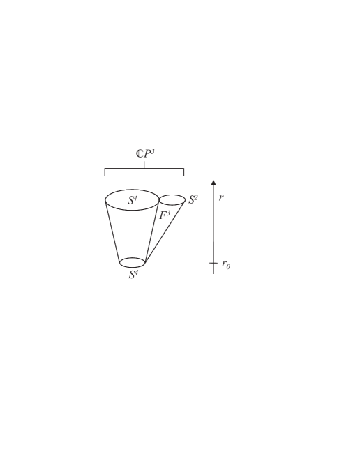
Figure 7.1: Another non-compact $G_{2}$-manifold.

An important property of this metric is that if differs from a conical metric by terms of order $(r_{0}/r)^{4}$, for $r\rightarrow\infty$. The consequence of this fact is that fluctuations of $r_{0}$ can be regarded as physical fields with finite kinetic energy. This comes about as follows. Let $\langle g\rangle$ be the metric as it is given above with fixed $\langle r_{0}\rangle$. Now suppose $r_{0}$ fluctuates as $r_{0}=\langle r_{0}\rangle+\delta r_{0}$. We write the corresponding metric as $g=\langle g\rangle+\delta g$. If we define the norm of $\delta g$ as

$$|\delta g|^{2}:=\int_{X}d^{7}x\sqrt{g}g^{ii^{\prime}}g^{jj^{\prime}}\delta g_{ij}\delta g_{i^{\prime}j^{\prime}}$$ (7.14)

we find that

$$|\delta g|^{2}<\infty,$$ (7.15)

as $\delta g/g\sim r^{-4}$ and we integrate over a seven-dimensional space. This means that in M-theory on $\mathbb{R}^{4}\times X$ the kinetic energy associated with fluctuations of $r_{0}$ is finite and they can be considered as a physical field.
It is interesting to see, that the fields corresponding to a fluctuation of $r_{0}$ really live only close to the tip of the cone. Denote $g(\langle r_{0}\rangle):=g_{\langle r_{0}\rangle}(x,y,r)$ the metric on the entire space $\mathbb{R}^{4}\times X$. Then we get the variation of the metric

$$\delta g=g(\langle r_{0}\rangle+\delta r_{0}(x))-g(\langle r_{0}\rangle)={\delta g\over\delta r_{0}}\Big{|}_{\langle r_{0}\rangle}\delta r_{0}(x).$$ (7.16)

But from the explicit form of the metric (7.12) we see that $\delta g$ gets small for large values of $r$ and is of order one for $r\sim\langle r_{0}\rangle$. We conclude that in the case of a singular space with $\langle r_{0}\rangle=0$ the fluctuations are four-dimensional fields only present on the singularity. In particular, if we start from a space with more than one singularities there will be a four-dimensional field at each of them. These fields do not interact, as they live in different four-dimensional spaces - their “$r$-coordinate” is different.
As we ensured that our theory has $\mathcal{N}=1$ supersymmetry by compactifying on a $G_{2}$-manifold, we expect that this fields should have supersymmetric partners. Indeed there is a contribution from the $C$-field which gives another scalar field in four dimensions. The mechanism leading to this field is by now familiar. On the space (7.12) there is one $L^{2}$-harmonic three-form $\Omega$ [12] and we get $C=\phi\Omega+\ldots$ . These two fields combine to a complex scalar as

$$z=V\exp\left(i{T_{2}}\int_{F^{3}}\widetilde{C}\right),$$ (7.17)

where $V\propto r_{0}^{4}$ is the volume of the $S^{4}$ at the center of our space and the integral is over one fibre of $X\rightarrow S^{4}$. The field $\widetilde{C}$ will be described in detail in the next chapter. It vanishes close to the tip of the cone where the curvature is large and equals $C$ away from the tip of the cone. Its most important property is its transformation under gauge variation $\delta\widetilde{C}=\Lambda\wedge\delta(r-R)dr+\ldots$ for some positive parameter $R$.
The corresponding superpartner to this complex bosonic field is a chiral fermion. Again it should be emphasized that if we start with $\langle r_{0}\rangle=0$ we get a fermion living on the singularity of our space. So we conclude that a “compactification” of M-theory on (7.12) leads to a chiral multiplet in four dimensions, which carries the additional label $\langle r_{0}\rangle$.
So far anything we did is familiar, as we should expect $b^{3}(X)$ neutral chiral multiplets in our manifold, according to the considerations of section 5.3. However, something new will happen in the case when we take $\langle r_{0}\rangle=0$, that is when we really choose the vacuum on which we compactify to be singular. To see this we need to study the symmetries of this model.
In principle we need to study both geometrical symmetries and symmetries coming from the $C$-field. However, it turns out that geometrical symmetries are not very important for this particular model as all the symmetries of $Y$ extend over $X$ [12]. The important symmetry in our case comes from the $C$-field. As we have $b^{2}(Y)=1$ the symmetry of the theory is given by $U(1)\cong H^{2}(Y;U(1))$. But $b^{2}(X)=0$ which tells us that this symmetry is broken to nothing.
It is natural to expect that the Betti numbers of $Y$ and $X$ are different as long as $X$ is smooth. This can be understood easily by looking at a simple model. Consider the first homology group of $S^{1}$ and the upper half of a sphere $S^{2}_{+}$ which is bounded by $S^{1}$. Certainly $H_{1}(S^{1};\mathbb{Z})=\mathbb{Z}$ but $H_{1}(S^{2}_{+};\mathbb{Z})=0$. This is clear as on $S^{2}_{+}$ any circle is contractible. But now consider what happens if we deform $S^{2}_{+}$ until it is a cone on $S^{1}$, $C(S^{1})$. Then it is no longer true that we can contract any circle to a point, as we have a singularity at the tip of the cone. Hence, we can introduce a winding number and $H_{1}(C(S^{1});\mathbb{Z})=\mathbb{Z}$. But this is exactly what happens in the case when we take $\langle r_{0}\rangle$ to vanish. In this case the cohomology groups of $Y$ and $X$ are isomorphic and we conclude that the $U(1)$ symmetry is restored. The crucial point is that the chiral multiplet is charged under the corresponding gauge field [12]. To see this we need to consider the Kaluza-Klein expansion of $C$. As long as $X$ is non-singular we have no harmonic two-forms and thus no massless gauge fields in four dimensions. The situation changes if $X$ becomes singular. Then we have $H^{2}(X;U(1))\cong H^{2}(Y;U(1))\cong U(1)$ and we can expand $C=A\wedge\omega+\ldots$, so in the case of singular manifolds a new gauge field arises. For the case of compact weak $G_{2}$-manifolds with conical singularities the isomorphism $H^{2}(X;U(1))\cong H^{2}(Y;U(1))$ was proven in [22]. Under a gauge transformation of this field we have

$$z^{\prime}=V\exp\left(i{T_{2}}\int_{F^{3}}(\widetilde{C}+\Lambda\wedge\delta(r-R)dr)\right)=e^{i{\epsilon(x)}}V\exp\left(i{T_{2}}\int_{F^{3}}\widetilde{C}\right),$$ (7.18)

where we used $\Lambda=\epsilon\omega+\ldots$ and $\int_{S^{2}}T_{2}\omega=1$. But this is exactly the transformation law of a charged chiral multiplet. Of course, in order to write down a gauge invariant Lagrangian we need to introduce a covariant derivative which couples the fermions to the new gauge field. Hence, in the case of singular $G_{2}$-manifolds we really obtained chiral multiplets which couple to gauge fields.
Let us summarize what we have done so far. We saw that the compactification of M-theory on a smooth $G_{2}$-manifold that is asymptotic to a cone on $\mathbb{CP}^{3}$ gives us $b^{2}(X)=0$ Abelian vector multiplets and $b^{3}(X)=1$ neutral chiral multiplets. This is exactly as expected from the analysis of section 5.3. However, in the limit in which the manifolds becomes singular a new four-dimensional Abelian gauge field arises and we were able to show, that this gauge field couples to the chiral multiplet present at the singularity. So we really obtained charged chiral fermions from compactifications on singular spaces. But of course these fields in general lead to anomalies. So we have to study whether M-theory on singular $G_{2}$-manifolds is anomaly free. This will be done in the next chapter.

Finally we want to mention that it is possible to get chiral fermions from compactifications of M-theory on singular $G_{2}$-manifolds which couple to non-Abelian gauge fields. We saw already, that is necessary to have $ADE$ singularities localized at $Q$ in $X$ to obtain non-Abelian gauge groups. In general $Q$ is a three-dimensional submanifold of $X$ but it might happen that $Q$ itself develops a singularity. Close to these singularities $X$ looks like a cone and we expect a chiral multiplet from its fluctuations. In fact in this case the multiplet is charged under the relevant $ADE$ gauge group. See [12], [87] and [4] for the details of this mechanism. In these references an explicit example is given involving a cone on a weighted projective space. We will comment on the anomaly structure of these spaces in section 8.2.

Chapter 8 Anomaly Analysis of M-Theory on $G_{2}$-Manifolds

In the last chapter we showed that it is possible to obtain realistic theories from compactifications of M-theory on singular $G_{2}$-manifolds. We obtained four-dimensional chiral fermions which are charged under Abelian or non-Abelian gauge groups. So in a sense we reached our goal of constructing realistic theories from M-theory. However, once this is done we obviously need to check whether this theory is really consistent. In general chiral fermions give rise to anomalies and these have to cancel in a well-defined theory. The idea of how this might occur was first developed in [87], however, we present the modified version of [23].

8.1 Chiral Fermions from Anomaly Considerations

Let $X$ be a compact $G_{2}$-manifold that is smooth except for conical singularities. Up to now it is not clear whether compact $G_{2}$-manifolds of that kind exist, however, examples of non-compact spaces with conical singularities are known [49]. The term manifold should be taken with a grain of salt, as the space has a singularity and hence cannot be a Riemannian manifold in the strict sense. However, it can be viewed as a limiting point in the moduli space of $G_{2}$-metrics. For example the non-compact $G_{2}$-metrics of (2.23) and (7.12) develop a conical singularity in the limit in which $r_{0}\rightarrow 0$.

Figure 8.1: A smooth $G_{2}$-manifold develops a conical singularity.

We saw in the last chapter that for certain geometries there are four-dimensional charged chiral fermions sitting on the singularities $P_{\alpha}$, with $\alpha$ a label running over the number of singularities in $X$. From anomaly cancellation we will learn that these fermions are of negative chirality. These lead to a variation of the Euclidean quantum effective action of the form

$$\delta X|_{anomaly}=-2\pi i\hat{I}_{4}^{1}\ \ \mbox{with}\ \ \hat{I}_{6}=(-1)[\hat{A}(M_{4}){\rm ch}(F)]_{6}.$$ (8.1)

The Euclidean gauge anomaly localized at $P_{\alpha}$ is (recall that $I=-2\pi\hat{I}$ and $F=iF^{i}q^{i}$),

$$I_{\alpha}^{(gauge)}=-{1\over(2\pi)^{2}3!}\sum_{\sigma\in T_{\alpha}}\left(\sum_{i=1}^{b^{2}(X)}q_{\sigma}^{i}F^{i}\right)^{3}.$$ (8.2)

$\sigma$ labels the four dimensional chiral multiplets $\Phi_{\sigma}$ which are present at the singularity $P_{\alpha}$. $T_{\alpha}$ is simply a set containing all these labels. $q_{\sigma}^{i}$ is the charge of $\Phi_{\sigma}$ with respect to the $i$-th gauge field $A^{i}$. As all the gauge fields come from a Kaluza-Klein expansion of the $C$-field we have $b^{2}(X)$ of them. Clearly we get a mixed anomaly as well,

$$I_{\alpha}^{(mixed)}={1\over 24}\sum_{\sigma\in T_{\alpha}}\left(\sum_{i=1}^{b^{2}(X)}q_{\sigma}^{i}F^{i}\right)p_{1}^{\prime}.$$ (8.3)

Here $p_{1}^{\prime}=-{1\over 8\pi^{2}}\,{\rm tr}\,R\wedge R$ is the first Pontrjagin class of four dimensional space-time $\mathbb{R}^{4}$.
As usual the effective four-dimensional theory is obtained by integrating over the compact space $X$. But this means that the effective theory has anomalies

$$I^{(gauge)} = \sum_{\alpha}I_{\alpha}^{(gauge)},$$ (8.4)

$$I^{(mixed)} = \sum_{\alpha}I_{\alpha}^{(mixed)}.$$ (8.5)

Certainly, these anomalies have to cancel in a consistent theory. However, we saw already at various places that it is not sufficient to have global anomaly cancellation in M-theory. Instead anomalies have to be cancelled locally. This means that we need to find a mechanism, that cancels $I_{\alpha}^{(gauge)}$ and $I_{\alpha}^{(mixed)}$ at each singularity $P_{\alpha}$ separately.

All the “M-theory” calculations we performed so far actually used the action of eleven-dimensional supergravity together with some correction terms. However, in the neighbourhood of a conical singularity the curvature of $X$ blows up. Close to the singularity $X$ is a cone on some manifold $Y$. But as $X$ is Ricci-flat $Y$ has to be Einstein with $\mathcal{R}^{Y}_{mn}=5\delta_{mn}$. The Riemann tensor on $X$ and $Y$ are related by $R^{Xmn}_{\ \ \ \ \ pq}={1\over r^{2}}(R^{Ymn}_{\ \ \ \ \ pq}-\delta^{m}_{p}\delta^{n}_{q}+\delta^{m}_{q}\delta^{n}_{p})$, for $m\in\{1,2,\ldots,6\}$. Thus, the supergravity description is no longer valid close to a singularity and one has to resort to a full M-theory calculation, a task that is currently not feasible. To avoid this difficulty we could, following [87], excise the singularities of $X$, i.e. we could cut off the tips of all the cones in our manifold. Then we were left with a manifold with boundary $X^{\prime}$ such that

$$\partial X^{\prime}=-\cup_{\alpha}Y_{\alpha}.$$ (8.6)

$Y_{\alpha}$ is the component of the boundary of $X^{\prime}$ which comes from cutting out $P_{\alpha}$ and we chose its orientation to be opposite to the one induced by the boundary operator. In that way we get rid of those points with arbitrary large curvature and the supergravity approximation can be used for compactifications on $X^{\prime}$. So, the basic idea in [87] is to model the effect of a singularity by a boundary which arises from cutting off this singularity.

Figure 8.2: Excising the singularities gives a manifold with boundary.

We want to try to follow a similar but different route to study singular spaces. Suppose we start from M-theory on $\mathbb{R}^{4}\times X$ with $X$ carrying conical singularities. The expectation values of the $C$-field and the gravitino vanish for compactifications on $G_{2}$-manifolds, but we allow for fluctuations. We are only interested in fluctuations of the three-form, which we will denote $C_{0}$. The corresponding field strength is given by $G_{0}=dC_{0}$. As we discussed above we cannot do supergravity calculations in this setup.
But now suppose that the fields can be shielded by some mechanism close to the singularities. That is we introduce some arbitrary parameter $R$ and a new set of fields $\{C,G\}$ on $X$ with two important properties. Firstly we want them to vanish at points which are closer to a singularity than $R$. Secondly, they are given by the original fields $\{C_{0},G_{0}\}$ for distances bigger than $R$. Note that we do not introduce a new metric but we want to keep fixed the geometry of our setup. The aim is to understand the dynamics of the new set of fields $\{C,G\}$ on $X$, which can be done using supergravity.
The mathematical formulation of this is as follows. Choose a set of charts on $X$ such that the neighbourhood of each singularity is covered by a single chart. On this chart the metric is conical and there is a natural coordinate $r_{\alpha}$ for each $P_{\alpha}$. Next we introduce a set of smooth functions $\rho_{\alpha}$ on the chart around $P_{\alpha}$ with the properties

$$\rho_{\alpha}(r_{\alpha})=\left\{\begin{matrix}0&\mbox{for}&\ \ 0\leq r_{\alpha}\leq R-\epsilon\\ 1&\mbox{for}&r_{\alpha}\geq R+\epsilon\end{matrix}\right.$$ (8.7)

where $\epsilon/R$ is small.
Using a partition of unity we can construct a smooth function $\rho$ on $X$ from these $\rho_{\alpha}$ in such a way that $\rho$ vanishes for points with a distance to a singularity which is less than $R-\epsilon$ and is one for distances larger than $R+\epsilon$. We denote the points of radial coordinate $R$ in the chart around $P_{\alpha}$ by $Y_{\alpha}$ and the subspace of $X$ which is bounded by these $Y_{\alpha}$ is denoted $X^{\prime}$. All these conventions are chosen in such a way that $\int_{X}(\ldots)\wedge d\rho=\sum_{\alpha}\int_{Y_{\alpha}}(\ldots)$. This clarifies the relation of the current approach to the one used in [87]. Our model can be understood as the embedding of a manifold with boundary into a manifold.
Now we want to impose the following boundary conditions on the fields of our new theory

$$C = \left\{\begin{matrix}0&\mbox{for one}&r_{\alpha}<R-\epsilon\\ C_{0}&\mbox{for all}&r_{\alpha}>R+\epsilon\end{matrix}\right.$$ (8.8)

$$G = \left\{\begin{matrix}0&\mbox{for one}&r_{\alpha}<R-\epsilon\\ G_{0}&\mbox{for all}&r_{\alpha}>R+\epsilon\end{matrix}\right.$$ (8.9)

So what did we gain from introducing this new theory on $\mathbb{R}^{4}\times X$ with a new set of fields? The important property of this theory is, that it reproduces the results of the theory with the field content $\{C_{0},G_{0}\}$ for distances from the singularities larger than $R$. The basic setup is shown in figure (8.3).

Figure 8.3: Embedding a manifold with boundary into a manifold.

Let us analyze the consequences of this situation. Most importantly, it is clear that we have to introduce a source for the $G$-field at $R$. We need to have

$$dG=G_{0}\wedge d\rho.$$ (8.10)

Note that the strength of the source is given by the value of $G_{0}$ on $Y_{\alpha}$. If we worked with a manifold with boundary we certainly would need to impose boundary conditions on $Y_{\alpha}$. In our model, there is no boundary, but (8.10) is necessary for the $G$-field to satisfy our requirements. So our model leads to a modified Bianchi identity, very much in the spirit of the chapters 4 and 6. The general solution of this equation is given by

$$G=aG_{0}\rho+(1-a)C_{0}\wedge d\rho+bH_{4}+cdC_{3}+edB\wedge d\rho.$$ (8.11)

Here $\{a,b,c,e\}$ are real coefficients, $H_{4}$ is a harmonic four-form on $X$, $C_{3}$ is a three-form on $\mathbb{R}^{4}\times X$ and $B$ is an arbitrary two-form on $\mathbb{R}^{4}\times X$. Note, however, that $d\rho$ has support only close to the $Y_{\alpha}$, so one might have introduced a set of independent two-forms $B_{\alpha}$ on $\mathbb{R}^{4}\times Y_{\alpha}$. In that case the last term would read $\sum_{\alpha}dB_{\alpha}\wedge d\rho$. Imposing the boundary conditions (8.9) gives the simple solution

$$G=G_{0}\rho.$$ (8.12)

The gauge invariant kinetic term of our theory is constructed from this field

$$S_{kin}=-{1\over 4\kappa_{11}^{2}}\int G\wedge\star G=-{1\over 4\kappa_{11}^{2}}\int_{r\geq R}dC_{0}\wedge\star dC_{0}.$$ (8.13)

To proceed we need to recall what we did in the presence of a modified Bianchi identity in chapter 6. There the $G$-field which occurred in the topological term in the supergravity action had to be corrected in a way that $d(G+$corrections)=0. Applying this to our model we define yet another field

$$\widetilde{G} := G-(C_{0}-dB)\wedge d\rho$$ (8.14)

$$= G_{0}\rho-(C_{0}-dB)\wedge d\rho$$

$$= d\left(C_{0}\rho+B\wedge d\rho\right)$$

$$=: d\widetilde{C}$$

and postulate a modified topological term of the form

$$\widetilde{S}_{top} := -{1\over 12\kappa_{11}^{2}}\int_{\mathbb{R}^{4}\times X}\widetilde{C}\wedge\widetilde{G}\wedge\widetilde{G}$$ (8.15)

$$= -{2\pi\over 6}\left(T_{2}\over 2\pi\right)^{3}\int_{\mathbb{R}^{4}\times X}\widetilde{C}\wedge\widetilde{G}\wedge\widetilde{G}.$$ (8.16)

Here we used the identity (6.24) which is always valid in M-theory. It is interesting to analyze the structure of this term,

$$\widetilde{S}_{top} = -{2\pi\over 6}\left(T_{2}\over 2\pi\right)^{3}\int_{\mathbb{R}^{4}\times X}\widetilde{C}\wedge\widetilde{G}\wedge\widetilde{G}$$ (8.17)

$$= -{2\pi\over 6}\left(T_{2}\over 2\pi\right)^{3}\int_{\mathbb{R}^{4}\times X}(C_{0}\rho+B\wedge d\rho)\wedge$$

$$\wedge(G_{0}\rho-(C_{0}-dB)\wedge d\rho)\wedge(G_{0}\rho-(C_{0}-dB)\wedge d\rho)$$

$$= -{2\pi\over 6}\left(T_{2}\over 2\pi\right)^{3}\int_{\mathbb{R}^{4}\times X}\left(C_{0}\wedge G_{0}\wedge G_{0}\rho^{3}+\right.$$

$$\left.+2C_{0}\wedge dB\wedge G_{0}\wedge\rho^{2}d\rho+B\wedge G_{0}\wedge G_{0}\wedge\rho^{2}d\rho\right)$$

$$= -{2\pi\over 6}\left(T_{2}\over 2\pi\right)^{3}\int_{\mathbb{R}^{4}\times X}C_{0}\wedge G_{0}\wedge G_{0}\rho^{3}$$

$$-{1\over 3}\sum_{\alpha}{2\pi\over 6}\left(T_{2}\over 2\pi\right)^{3}\int_{\mathbb{R}^{4}\times Y_{\alpha}}\left(2C_{0}\wedge dB\wedge G_{0}+B\wedge G_{0}\wedge G_{0}\right)$$

$$= -{2\pi\over 6}\left(T_{2}\over 2\pi\right)^{3}\int_{\mathbb{R}^{4}\times X}C_{0}\wedge G_{0}\wedge G_{0}\rho^{3}$$

$$-\sum_{\alpha}{2\pi\over 6}\left(T_{2}\over 2\pi\right)^{3}\int_{\mathbb{R}^{4}\times Y_{\alpha}}B\wedge G_{0}\wedge G_{0}.$$

Here we used that $\rho^{2}d\rho\rightarrow{1\over 3}d\rho$. So we have the usual topological term on $X^{\prime}$, nothing close to the singularities and a contribution $BG_{0}G_{0}$ on each $Y_{\alpha}$. This additional term is rather interesting and we will give some speculative comments related to it in the next chapter. Of course the whole construction is similar in spirit to what we did in chapter 6 and clearly the structure of the modified topological term is similar in both cases.
The field $\widetilde{G}$ is closed by construction but, because of its position in the topological term, we also want it to be gauge invariant. This gives us the transformation law of $B$,

$$0 = \delta\widetilde{G}=d\left(d\Lambda\rho+\delta B\wedge d\rho\right)$$ (8.18)

$$= (d\delta B-d\Lambda)\wedge d\rho,$$

from which we read off

$$\delta B=\Lambda.$$ (8.19)

Then it is easy to write down the transformation law of $\widetilde{C}$,

$$\delta\widetilde{C} = \delta C_{0}\rho+\delta B\wedge d\rho$$ (8.20)

$$= d\Lambda\rho+\Lambda\wedge d\rho$$

$$= d(\Lambda\rho).$$

Now we are ready to calculate the gauge transformation of the modified topological term. It reads

$$\delta\widetilde{S}_{top} = -{2\pi\over 6}\left(T_{2}\over 2\pi\right)^{3}\int_{\mathbb{R}^{4}\times X}\delta\widetilde{C}\wedge\widetilde{G}\wedge\widetilde{G}$$ (8.21)

$$= -{2\pi\over 6}\left(T_{2}\over 2\pi\right)^{3}\int_{\mathbb{R}^{4}\times X}d(\Lambda\rho)\wedge(G_{0}\rho-(C_{0}-dB)\wedge d\rho)\wedge(G_{0}\rho-(C_{0}-dB)\wedge d\rho)$$

$$= -{2\pi\over 6}\left(T_{2}\over 2\pi\right)^{3}\int_{\mathbb{R}^{4}\times X}d\Lambda\wedge G_{0}\wedge G_{0}\rho^{3}$$

$$+2{2\pi\over 6}\left(T_{2}\over 2\pi\right)^{3}\int_{\mathbb{R}^{4}\times X}d\Lambda\wedge G_{0}\wedge(C_{0}-dB)\wedge\rho^{2}d\rho-$$

$$-{2\pi\over 6}\left(T_{2}\over 2\pi\right)^{3}\int_{\mathbb{R}^{4}\times X}\Lambda\wedge G_{0}\wedge G_{0}\wedge\rho^{2}d\rho.$$

We substitute the Kaluza-Klein expansions

$$C_{0}(x,y) = \sum_{i}A^{i}(x)\wedge\omega^{i}(y)+\ldots,$$ (8.22)

$$\Lambda(x,y) = \sum_{i}\epsilon^{i}(x)\omega^{i}(y)+\ldots,$$ (8.23)

$$B(x,y) = \sum_{i}\phi^{i}(x)\omega^{i}(y)+\ldots,$$ (8.24)

and get

$$\delta\widetilde{S}_{top} = {2\over 3}{2\pi\over 6}\left(T_{2}\over 2\pi\right)^{3}\int_{\mathbb{R}^{4}\times X}d\epsilon^{i}F^{j}(A^{k}-d\phi^{k})\omega^{i}\wedge\omega^{j}\wedge\omega^{k}\wedge d\rho$$ (8.25)

$$-{1\over 3}{2\pi\over 6}\left(T_{2}\over 2\pi\right)^{3}\int_{\mathbb{R}^{4}\times X}\epsilon^{i}F^{j}F^{k}\omega^{i}\wedge\omega^{j}\wedge\omega^{k}\wedge d\rho+\ldots$$

$$= {2\over 3}\sum_{\alpha}{2\pi\over 6}\left(T_{2}\over 2\pi\right)^{3}\int_{\mathbb{R}^{4}\times Y_{\alpha}}d\epsilon^{i}F^{j}(A^{k}-d\phi^{k})\omega^{i}\wedge\omega^{j}\wedge\omega^{k}$$

$$-{1\over 3}\sum_{\alpha}{2\pi\over 6}\left(T_{2}\over 2\pi\right)^{3}\int_{\mathbb{R}^{4}\times Y_{\alpha}}\epsilon^{i}F^{j}F^{k}\omega^{i}\wedge\omega^{j}\wedge\omega^{k}+\ldots$$

$$= {2\over 3}\sum_{\alpha}{2\pi\over 6}\left(T_{2}\over 2\pi\right)^{3}\int_{\mathbb{R}^{4}}d\epsilon^{i}F^{j}(A^{k}-d\phi^{k})\int_{Y_{\alpha}}\omega^{i}\wedge\omega^{j}\wedge\omega^{k}$$

$$-{1\over 3}\sum_{\alpha}{2\pi\over 6}\left(T_{2}\over 2\pi\right)^{3}\int_{\mathbb{R}^{4}}\epsilon^{i}F^{j}F^{k}\int_{Y_{\alpha}}\omega^{i}\wedge\omega^{j}\wedge\omega^{k}+\ldots$$

$$= -\sum_{\alpha}{1\over(2\pi)^{2}3!}\int_{\mathbb{R}^{4}}\epsilon^{i}F^{j}F^{k}\int_{Y_{\alpha}}(T_{2})^{3}\omega^{i}\wedge\omega^{j}\wedge\omega^{k}+\ldots$$

Note that substituting the Kaluza-Klein expansions into $d\Lambda\wedge G_{0}\wedge G_{0}$ gives zero. Furthermore, we integrated by parts on $\mathbb{R}^{4}$ to obtain the last equation. The result is a sum of terms which are localized at $Y_{\alpha}$. The corresponding Euclidean anomaly polynomial is given by

$$I^{(top)}_{E}=\sum_{\alpha}I^{(top)}_{E,\alpha}=-i\sum_{\alpha}I^{(top)}_{M,\alpha}=\sum_{\alpha}{i\over(2\pi)^{2}3!}F^{i}F^{j}F^{k}\int_{Y_{\alpha}}(T_{2})^{3}\omega^{i}\wedge\omega^{j}\wedge\omega^{k}+\ldots$$ (8.26)

This is very similar to the gauge anomaly $I_{\alpha}^{(gauge)}$ and we do indeed get a local cancellation of the anomaly provided we have

$$\int_{Y_{\alpha}}(T_{2})^{3}\omega^{i}\wedge\omega^{j}\wedge\omega^{k}=\sum_{\sigma\in T_{\alpha}}q_{\sigma}^{i}q_{\sigma}^{j}q_{\sigma}^{k}.$$ (8.27)

(Note that the condition of local anomaly cancellation is $iI_{\alpha}^{(gauge)}+I^{(top)}_{E,\alpha}=0$, from (3.142).) In [87] it was shown that this equation holds for all known examples of conical singularities. Note that the dimensions of (8.27) are correct. We have $[(C_{0})_{\mu mn}]=0$ but $[A_{\mu}]=1$, therefore $[\omega_{mn}]=-1$, hence we need a factor of dimension nine on the left-hand side to give us a dimensionless quantity.
Turning things around, had we not known that there are charged (anti-)chiral fermions living on the singularity we would be forced to introduce them at this point in order to cancel the anomalies of our theory. Their charges would be constraint to satisfy the condition (8.27), thus we conclude that it depends on the geometry of the manifold $X$ and in particular on the properties of the harmonic two-forms on $X$ whether chiral fermions are present or not.
It is particularly important that our modified topological term gave us a sum of terms localized at $Y_{\alpha}$ without any integration by parts on $X$. This is crucial, because local quantities are no longer well-defined after an integration by parts. In fact let us consider once again the variation of the topological term and let us this time integrate by parts.

$$\delta\widetilde{S}_{top}=-{2\pi\over 6}\left(T_{2}\over 2\pi\right)^{3}\int d(\Lambda\rho)\wedge\widetilde{G}\wedge\widetilde{G}=2{2\pi\over 6}\left(T_{2}\over 2\pi\right)^{3}\int\Lambda\rho\wedge d\widetilde{G}\wedge\widetilde{G}=0,$$ (8.28)

as $d\widetilde{G}=0$. Hence, $I^{(top)}_{E}=\sum_{\alpha}I^{(top)}_{E,\alpha}=0$, the gauge variation of the topological term vanishes. But this is a global statement, as we saw explicitly that $\widetilde{S}_{top}$ is a sum of terms located at $Y_{\alpha}$. This tells us that the situation is rather subtle. We have the anomalies $I_{\alpha}^{(gauge)}$, $I_{E,\alpha}^{(top)}$, $I^{(gauge)}$ and $I^{(top)}_{E}$ with $I^{(top)}_{E}=\sum_{\alpha}I_{E,\alpha}^{(top)}$, $I^{(gauge)}=\sum_{\alpha}I_{\alpha}^{(gauge)}$ and $I_{E,\alpha}^{(top)}=-iI_{\alpha}^{(gauge)}$. But we just showed that $I^{(top)}_{E}=0$, so $I^{(gauge)}=\sum_{\alpha}I_{\alpha}^{(gauge)}=i\sum_{\alpha}I_{E,\alpha}^{(top)}=iI^{(top)}_{E}=0$, the global gauge anomaly vanishes as well.
Clearly in this situation the concept of local and global anomalies is very important. We just saw that the sum of all the anomalies in a theory with an unmodified topological term vanishes, i.e. the anomalies vanish after integration over $X$. Although this is what we will do in the end to obtain a four-dimensional theory it is not sufficient. In fact the anomalies are localized at the singularities as the chiral fermions live only there. These localized anomalies have to be cancelled before we integrate over the compact space. The modification of the topological term is done in such a way that the anomalies cancel independently at each singularity.

After having seen how anomaly cancellation works in the case of gauge anomalies we turn to the mixed anomaly. We start by considering the Green-Schwarz term in a theory on a smooth manifold $\mathbb{R}^{4}\times X$. It can be rewritten as

$$S_{GS}=-{T_{2}\over 2\pi}\int_{\mathbb{R}^{4}\times X}G_{0}\wedge X_{7}=-{T_{2}\over 2\pi}\int_{\mathbb{R}^{4}\times X}C_{0}\wedge X_{8},$$ (8.29)

with $X_{8}$ as in (4.16) and $X_{8}=dX_{7}$. The coefficient was determined from the anomaly cancellation condition in chapter 6 and is consistent with the results of chapter 4.
Then, there is a natural modification of the Green-Schwarz term on our singular manifold,

$$\widetilde{S}_{GS}:=-{T_{2}\over 2\pi}\int_{\mathbb{R}^{4}\times X}\widetilde{C}\wedge X_{8}.$$ (8.30)

As before it is interesting to study the detailed structure of this term,

$$\widetilde{S}_{GS} = -{T_{2}\over 2\pi}\int_{\mathbb{R}^{4}\times X}(C_{0}\rho+B\wedge d\rho)\wedge X_{8}$$ (8.31)

$$=-{T_{2}\over 2\pi}\int_{\mathbb{R}^{4}\times X}C_{0}\rho\wedge X_{8}-{T_{2}\over 2\pi}\sum_{\alpha}\int_{\mathbb{R}^{4}\times Y_{\alpha}}B\wedge X_{8}.$$

Once again we get the usual term in the bulk, nothing close to the singularities and a very special contribution from the $Y_{\alpha}$.
The variation of the Green-Schwarz term is easily calculated,

$$\delta\widetilde{S}_{GS} = -{T_{2}\over 2\pi}\int_{\mathbb{R}^{4}\times X}\delta\widetilde{C}\wedge X_{8}$$ (8.32)

$$= -{T_{2}\over 2\pi}\int_{\mathbb{R}^{4}\times X}d(\Lambda\rho)\wedge X_{8}$$

$$= -{T_{2}\over 2\pi}\int_{\mathbb{R}^{4}\times X}d\Lambda\rho\wedge X_{8}-{T_{2}\over 2\pi}\int_{\mathbb{R}^{4}\times X}\Lambda\wedge d\rho\wedge X_{8}$$

$$= -{T_{2}\over 2\pi}\int_{\mathbb{R}^{4}\times X}d\Lambda\rho\wedge X_{8}-{T_{2}\over 2\pi}\sum_{\alpha}\int_{\mathbb{R}^{4}\times Y_{\alpha}}\Lambda\wedge X_{8}$$

$$= -{T_{2}\over 2\pi}\sum_{\alpha}\int_{\mathbb{R}^{4}\times Y_{\alpha}}\epsilon^{i}\omega^{i}\wedge X_{8}+\ldots.$$

To obtain the last line we used the Kaluza-Klein expansion (8.23) and the structure of $X_{8}$. As we saw in chapter 6, $X_{8}$ can be rewritten in terms of the first and second Pontrjagin class

$$p_{1} = -{1\over 2}\left({1\over 2\pi}\right)^{2}{\rm tr}R^{2},$$ (8.33)

$$p_{2} = {1\over 8}\left(1\over 2\pi\right)^{4}[({\rm tr}R^{2})^{2}-2{\rm tr}R^{4}],$$ (8.34)

as

$$X_{8}={\pi\over 4!}\left[{p_{1}^{2}\over 4}-p_{2}\right].$$ (8.35)

The background we are working in is four-dimensional Minkowski space times a $G_{2}$-manifold. In this special setup the Pontrjagin classes can easily be expressed in terms of the Pontrjagin classes $p_{i}^{\prime}$ on $(\mathbb{R}^{4},\eta)$ and those on $(X,g)$, which we will write as $p_{i}^{\prime\prime}$. We get

$$p_{1} = p_{1}^{\prime}+p_{1}^{\prime\prime}$$ (8.36)

$$p_{2} = p_{1}^{\prime}\wedge p_{1}^{\prime\prime}.$$ (8.37)

Using these relations we obtain a convenient expression for the inflow (8.32),

$$\delta\widetilde{S}_{GS} = -{T_{2}\over 2\pi}\sum_{\alpha}\int_{\mathbb{R}^{4}\times Y_{\alpha}}\epsilon^{i}\omega^{i}\wedge X_{8}$$ (8.38)

$$= -{T_{2}\over 2\pi}\sum_{\alpha}\int_{\mathbb{R}^{4}\times Y_{\alpha}}\epsilon^{i}\omega^{i}\wedge{\pi\over 4!}\left[{p_{1}^{2}\over 4}-p_{2}\right]$$

$$= -{T_{2}\over 2\pi}{\pi\over 4!}\sum_{\alpha}\int_{\mathbb{R}^{4}\times Y_{\alpha}}\epsilon^{i}\omega^{i}\wedge\left[{1\over 2}p_{1}^{\prime}\wedge p_{1}^{\prime\prime}-p_{1}^{\prime}\wedge p_{1}^{\prime\prime}\right]$$

$$= {T_{2}\over 2\pi}{\pi\over 48}\sum_{\alpha}\int_{\mathbb{R}^{4}}\epsilon^{i}p_{1}^{\prime}\int_{Y_{\alpha}}\omega^{i}\wedge p_{1}^{\prime\prime}.$$

The corresponding anomaly polynomial is given by

$$I^{(GS)}_{E}=\sum_{\alpha}I^{(GS)}_{E,\alpha}=-i\sum_{\alpha}{1\over 24}F^{i}p_{1}^{\prime}\int_{Y_{\alpha}}{T_{2}\over 4}\omega^{i}\wedge p_{1}^{\prime\prime},$$ (8.39)

and we see that the mixed anomaly cancels locally provided we have

$$\int_{Y_{\alpha}}{T_{2}\over 4}\omega^{i}\wedge p_{1}^{\prime\prime}=\sum_{\sigma\in T_{\alpha}}q_{\sigma}^{i}.$$ (8.40)

All known examples satisfy this requirement. Once again turning things around (8.40) might be seen as a second condition which has to be satisfied by the charges of the chiral fermions which have to be present on the singularities to have a well-defined theory.
Note that from integration by parts,

$$\delta\widetilde{S}_{GS}=-{T_{2}\over 2\pi}\int_{\mathbb{R}^{4}\times X}d(\Lambda\rho)\wedge X_{8}={T_{2}\over 2\pi}\int_{\mathbb{R}^{4}\times X}\Lambda\rho\wedge dX_{8}=0.$$ (8.41)

This tells us that $0=I^{(GS)}_{E}=\sum_{\alpha}I^{(GS)}_{E,\alpha}=\sum_{\alpha}-iI^{(mixed)}_{\alpha}=-iI^{(mixed)}$. The sum of all mixed anomalies vanishes.

The example of $\mathbb{CP}^{3}$

We saw that the anomalies of chiral fermions sitting on the singularities of $G_{2}$-manifolds vanish provided their charges satisfy certain geometrical conditions, namely (8.27) and (8.40). In the last chapter we studied the example of a manifold which is asymptotic to a cone on $\mathbb{CP}^{3}$. For this manifold we know both the geometry and the field content, thus we can check whether our conditions hold in this case. The fields were determined to consist of a single chiral multiplet with a charge that can be normalized to one. So the right-hand side of our conditions equals one. Let us check whether this is true for the left-hand side as well. We need to calculate

$$\int_{\mathbb{CP}^{3}}(T_{2})^{3}\omega^{i}\wedge\omega^{j}\wedge\omega^{k}$$

and

$${T_{2}\over 4}\int_{\mathbb{CP}^{3}}\omega^{i}\wedge p_{1}^{\prime\prime}.$$ (8.42)

We know that $b_{2}(\mathbb{CP}^{3})=1$, which is obvious from the fact that $\mathbb{CP}^{3}$ can be considered as an $S^{2}$-bundle over $S^{4}$. From de Rham’s theorem we derive that $b^{2}(\mathbb{CP}^{3})=1$ and we only have a single harmonic two-form $\omega$. Poincaré’s duality tells us that there is a single harmonic four-form $\Omega$ which can be normalized such that

$$T_{2}\int_{\mathbb{CP}^{3}}\omega\wedge\Omega=1.$$ (8.43)

But of course $\omega\wedge\omega$ is both closed and co-closed and thus $\omega\wedge\omega\propto\Omega$. This implies that choosing the normalization of $\omega$ appropriately we get

$$\int_{\mathbb{CP}^{3}}(T_{2})^{3}\omega\wedge\omega\wedge\omega=1.$$ (8.44)

Hence, (8.27) is satisfied in this example. The second condition can be verified easily as well, if one considers the details of the geometry of $\mathbb{CP}^{3}$. In this space the first two Chern classes are given by $c_{1}=4T_{2}\omega$, $c_{2}=6(T_{2})^{2}\omega\wedge\omega$ and the first Pontrjagin class is $p_{1}^{\prime\prime}=c_{1}^{2}-2c_{2}$ [42], [87]. Given this geometrical data it is easy to do the integral, as we have $p_{1}^{\prime\prime}=4(T_{2})^{2}\omega\wedge\omega$ yielding

$${T_{2}\over 4}\int_{\mathbb{CP}^{3}}\omega\wedge p_{1}^{\prime\prime}=\int_{\mathbb{CP}^{3}}(T_{2})^{3}\omega\wedge\omega\wedge\omega=1,$$ (8.45)

which is the required result. In [87] it was shown that the equations (8.27) and (8.40) are in fact true for all known examples of singular $G_{2}$-manifolds.

8.2 Non-Abelian Gauge Groups and Anomalies

Finally we also want to comment on anomaly cancellation in the case of non-Abelian gauge groups. The calculations are relatively involved in this case and we refer the reader to [87] and [23] for the details. We only present the basic mechanism. We saw in chapter 7 that chiral fermions which are charged under non-Abelian gauge groups occur if the locus $Q$ of an $ADE$ singularity in a $G_{2}$-manifold $X$ develops a singularity. Close to such a singularity $P_{\alpha}$ of $Q$ the space $X$ looks like a cone on some $Y_{\alpha}$. If $U_{\alpha}$ denotes the intersection of $Q$ with $Y_{\alpha}$ then close to $P_{\alpha}$ $Q$ is a cone on $U_{\alpha}$. We saw that in this case there are $ADE$ gauge fields on $\mathbb{R}^{4}\times Q$ which reduce to non-Abelian gauge fields on $\mathbb{R}^{4}$ if we perform a Kaluza-Klein expansion on $Q$. On the $P_{\alpha}$ we have a number of chiral multiplets $\Phi_{\sigma}$ which couple to both the non-Abelian gauge fields and the Abelian ones, coming from the Kaluza-Klein expansion of the $C$-field. Thus, we expect to get a $U(1)^{3}$, $U(1)H^{2}$ and $H^{3}$ anomaly, where $H$ is the relevant $ADE$ gauge group. The relevant anomaly polynomial for this case is

$$I_{6}=-2\pi[(-1)\hat{A}(M){\rm ch}(F^{(Ab)}){\rm ch}(F)]_{6}$$ (8.46)

where $F^{(Ab)}:=iq^{i}F^{i}$ denotes the Abelian and $F$ the non-Abelian gauge field. Expansion of this formula gives four terms namely (8.2), (8.3) and

$$I^{(H^{3})} = -{i\over(2\pi)^{2}3!}{\rm tr}F^{3},$$ (8.47)

$$I^{(U(1)_{i}H^{2})} = {1\over(2\pi)^{2}2}q_{i}F_{i}{\rm tr}F^{2}.$$ (8.48)

The anomalies which are related to these polynomials via the descent formalism are

$$G^{H^{3}}[\epsilon;A] = -{i\over(2\pi)^{2}3!}\int_{\mathbb{R}^{4}}{\rm tr}\left\{\epsilon\ d\left(AdA+{1\over 2}A^{3}\right)\right\},$$ (8.49)

$$G^{U(1)_{i}H^{2}}[\epsilon,\epsilon_{i};A,A_{i}] = {q_{i}\over(2\pi)^{2}2}\int_{\mathbb{R}^{4}}\left(\beta\epsilon_{i}{\rm tr}F^{2}+(1-\beta)F_{i}{\rm tr}(\epsilon dA)\right).$$ (8.50)

The anomalies (8.49) and (8.50) are cancelled from the gauge variations of two terms which are present in our special setup [87], [23]. They read

$$\widetilde{S}_{1}=-{i\over 6(2\pi)^{2}}\int_{\mathbb{R}^{4}\times Q}K\wedge{\rm tr}(\widetilde{A}\widetilde{F}^{2}),$$ (8.51)

$$\widetilde{S}_{2}={T_{2}\over 2(2\pi)^{2}}\int_{\mathbb{R}^{4}\times Q}\widetilde{C}\wedge{\rm tr}\widetilde{F}^{2}.$$ (8.52)

Here $K$ is the curvature of a certain line bundle in our setup described in [87] and $\widetilde{A}$ and $\widetilde{F}$ are modified versions of $A$ and $F$, the gauge potential and field strength of the non-Abelian $ADE$ gauge field living on $\mathbb{R}^{4}\times Q$. The gauge variation of these fields is calculated in [23] to be exactly the one which is necessary to achieve local cancellation of all anomalies. The main steps are similar to what we did in the last chapter. The only difficulty comes from the non-Abelian nature of the fields which complicates the calculation.

Chapter 9 Summary and Conclusions

We have come a far way by now. Starting from M-theory, which is still far from being well-understood, we showed that there are vacua of the theory carrying all the characteristic features of the standard model. As it also contains gravity in a natural way, M-theory may well be a unifying theory of all the known forces in nature. The methods we used were sometimes rather complicated. The main reason is that we had to use relatively unfamiliar mathematics leaving the domain of smooth manifolds and differential geometry, which is familiar to physicists. A crucial ingredient of the model outlined are spaces carrying various singularities. Depending on the singularity involved, one or another feature of the standard model emerges. It is interesting to see that charged chiral fermions can only arise in the very special case of compactifications on spaces with conical singularities. In a sense, only if the singularity has codimension seven the $G_{2}$-structure can maintain its full power and force supersymmetry to be $\mathcal{N}=1$. For singularities with a smaller codimension more supersymmetry is conserved. But then we get $CPT$ self-conjugate and hence non-chiral spectra. The singularity required for non-Abelian gauge theories has a quite different nature. Here we need it to have codimension four in the $G_{2}$-manifold. Interestingly enough, these singularities can be characterized using the classification scheme of simply laced semi-simple Lie algebras.
At this point it should also be mentioned that almost all our calculations are done using the low-energy effective theory of M-theory, eleven-dimensional supergravity. It is amazing that we can get this far, knowing so little about the fundamental formulation of M-theory. One of the reasons why this is the case is that practically everything we did was classical. There are some first steps towards the quantum dynamics of M-theory on $G_{2}$-manifolds, see for example [12] and [3]. Given the limitations of space, time and the author’s competence we could not comment on these interesting developments. However, it is probably fair to say that there is still much to be done before a rigorous and hopefully simple theory of the quantum dynamics on $G_{2}$-manifolds can be formulated.
The only real quantum phenomenon we encountered were anomalies. These can be handled for two important reasons. First and most importantly, it is not necessary to know the full quantum behaviour of M-theory for being able to study its anomalies. The reason is, of course, that anomalies are an infrared effect, which can be read off from the low-energy effective action. Secondly, the calculation of anomalies is facilitated by their relation to topological quantities of the base manifolds of the theory. Therefore, they can be evaluated from index theorems. As a consequence, an anomaly only depends on the dimension of the base space and the kind of field under consideration. Hence, anomalies can be calculated for each field and dimension once and for all and the results can be used without having to perform further calculations. We have repeatedly seen that anomalies allow to probe the quantum regime of a given theory. In chapter 4 they were the basic reason why the duality between M-theory on $\mathbb{R}^{10}\times S^{1}/\mathbb{Z}_{2}$ and the $E_{8}\times E_{8}$ heterotic string could be established. There we obtained the Green-Schwarz term as a first quantum correction to the supergravity action. This term again played a crucial role in the case of anomaly cancellation of M-theory containing M5-branes. In that case another new ingredient had to be introduced. The topological term had to be modified to ensure the cancellation of the normal bundle anomaly. Another interesting feature of anomaly theory is the concept of local anomaly cancellation. M-theory is formulated in eleven dimensions, where there are no local gauge anomalies. The concept of local anomaly cancellation states that the theory needs to be anomaly free on any even-dimensional subspace of the eleven-dimensional base manifold which contains four-dimensional Minkowski space. It is not sufficient to have an anomaly-free theory after integration over the compact space. This important concept makes it possible to show that four-dimensional chiral fermions have to be present at conical singularities of a $G_{2}$-manifold, as long as the geometry of the cone satisfies certain requirements. This case is particularly subtle as, contrary to Hořava-Witten theory, the sums of all gauge and mixed anomalies vanish. Nevertheless, there is a local anomaly at each singularity which can be cancelled only if additional chiral fermions are included.
In various M-theory calculations another inconvenience was encountered, namely that the space under consideration was not a manifold, but a manifold with boundary. These are much less comfortable as, for example, the Atiyah-Singer index theory is no longer true, but we have to use the Atiyah-Patodi-Singer index theorem. Hence, the anomaly calculations which are usually done for manifolds without boundary need to be revised. In order to avoid this difficulty, we adopted an approach to study singular spaces which makes it not necessary to excise the singularities. In a sense we embedded a manifold with boundary into a manifold. All the fields were multiplied by a smooth function $\rho$, which is supposed to model the boundary. In that way we were led to a nice and natural mechanism of anomaly cancellation for singular $G_{2}$-manifolds. This idea was is presented in detail in [23].
At this point we cannot resist speculating on how this formalism might be modified. In chapter 8 we saw that there is a source for the $G$-field in the regime were the $\rho$-function changes rapidly. One interpretation of this might be that we have M5-branes in our theory, as they are the only sources for a $G$-field that are known in M-theory. We might think of them as being smeared over the ten-dimensional space-time to give a “charge density”, just as electrons can be distributed on a conducting surface. Further evidence for this speculation comes from the structure of the modified terms. We basically added two interaction terms to our theory which read $\int_{\mathbb{R}^{4}\times Y_{\alpha}}BG_{0}G_{0}$ and $\int_{\mathbb{R}^{4}\times Y_{\alpha}}BX_{8}$, with a field $B$ that transforms as $\delta B=\Lambda$. Comparing this to (6.7), one might be tempted to identify the field $B$ with the two-form $A_{(2)}$ living on the M5-brane. Taking up the idea of the Faraday cage, our model may indeed be such a cage for M-theory. The interpretation would be that M5-branes are distributed on the surface of this cage, which is given by the union of the $Y_{\alpha}$, in such a way that $G$ is zero close to the singularities. However, then we would need to consider the tangent and normal bundle anomaly of those M5-branes, a complicated task, which has not been performed so far.
Finally, we should like to comment on possible criticism of the approach we have taken. There are two main points which might cast doubt on the model outlined being a promising candidate for a realistic theory. One is that the space we constructed is one of many possibilities, and one might ask why nature should have chosen exactly this particular one. Secondly, one might argue that our chosen vacuum is not only one of many but it is totally unnatural. Had we chosen a generic point in moduli space of $G_{2}$-manifolds, it would not be very difficult to account for it, as one point has to be chosen after all. However, we do not want a generic point, but we choose a certain limit lying on the boundary of the moduli space. In a sense, after a lot of engineering and pulling and squashing the spaces in a way that they satisfy the conditions we want, we just manage to stay at the brink of moduli space, a result which might not be very satisfying.
It remains an open question whether this criticism is justified. One certainly hopes to find a mechanism in M-theory that singles out the specific vacuum we constructed. Yet, it should be emphasized that it is really amazing that it is possible at all to construct a realistic theory in the given setup. Certainly, there remain a lot of open questions, which we leave for future exploration.

Acknowledgements

This thesis was written under the joint supervision of Adel Bilal at the École Normale Supérieure in Paris and Julius Wess at the Ludwig-Maximilians-Universität in Munich. I would like to thank both of them for their guidance and support and Adel Bilal for his never ceasing patience, endless discussions and a fruitful collaboration.
Furthermore, I would like to thank Jean-Pierre Derendinger, Yacine Dolivet, Jean Iliopoulos, Dan Israel, Branislav Jurco, Thomas Klose, Ruben Minasian, Chris Pope and Ivo Sachs for discussions and useful comments.

Appendix A General Notation

The number of space-time dimensions is denoted by $d$.

Indices:

	World	Tangent space	Coordinates
$d=11$ space-time	$M,N,\ldots\in\{0,1,\ldots 10\}$	$A,B,\ldots\in\{0,1,\ldots 10\}$	$z^{M}$
$d=4$ space-time	$\mu,\nu,\ldots\in\{0,1,2,3\}$	$a,b,\ldots\in\{0,1,2,3\}$	$x^{\mu}$
$d=7$ internal space	$m,n,\ldots\in\{1,2,\ldots,7\}$	$\hat{m},\hat{n},\ldots\in\{1,2,\ldots,7\}$	$y^{m}$

The metric on flat space is given by

$$\eta:={\rm diag}(-1,1,\ldots 1),$$ (A.1)

curved metrics are denoted by $g_{MN}$, with $g:=|{\rm det}\ (g_{MN})|$.
The anti-symmetric tensor is defined as

$$\widetilde{\epsilon}_{012\ldots d-1} := {\widetilde{\epsilon}}^{\ 012\ldots d-1}:=+1,$$ (A.2)

$$\epsilon_{M_{1}\ldots M_{d}} := \sqrt{g}\ \widetilde{\epsilon}_{M_{1}\ldots M_{d}}.$$ (A.3)

That is, we define $\widetilde{\epsilon}$ to be the tensor density and $\epsilon$ to be the tensor. We obtain

$$\epsilon_{012\ldots d-1} = \sqrt{g}=e:=|{\rm det}\ e^{A}_{\ \ M}|,$$ (A.4)

$$\epsilon^{M_{1}\ldots M_{d}} = {\rm sig}(g){1\over{\sqrt{g}}}\ \widetilde{\epsilon}^{\ M_{1}\ldots M_{d}},\mbox{\ \ and}$$ (A.5)

$$\widetilde{\epsilon}^{\ M_{1}\ldots M_{r}P_{1}\ldots P_{d-r}}\widetilde{\epsilon}_{N_{1}\ldots N_{r}P_{1}\ldots P_{d-r}} = r!(d-r)!\delta^{[M_{1}\ldots M_{r}]}_{N_{1}\ldots N_{r}}.$$ (A.6)

$$A_{(M_{1}\ldots M_{l})} := {1\over l!}\sum_{\pi}A_{M_{\pi(1)}\ldots M_{\pi(l)}}$$ (A.7)

$$A_{[M_{1}\ldots M_{l}]} := {1\over l!}\sum_{\pi}{\rm sig}(\pi)A_{M_{\pi(1)}\ldots M_{\pi(l)}}$$ (A.8)

p-forms are defined with a factor of $p!$, e.g.

$$\omega:={1\over p!}\omega_{M_{1}\ldots M_{p}}dz^{M_{1}}\wedge\ldots\wedge dz^{M_{p}}.$$ (A.9)

The Hodge dual is defined as

$$*\omega={1\over p!(d-p)!}\,\omega_{M_{1}\ldots M_{p}}\ \epsilon^{M_{1}\ldots M_{p}}_{\phantom{M_{1}\ldots M_{p}}M_{p+1}\ldots M_{d}}\ dz^{M_{p+1}}\wedge\ldots\wedge dz^{M_{d}}\ .$$ (A.10)

$[n]$ denotes the integer part of $n$.

Appendix B Spinors

B.1 Clifford Algebras and their Representation

Definition B.1
A Clifford algebra in $d$ dimensions is defined as a set containing $d$ elements $\Gamma^{A}$ which satisfy the relation

$$\{\Gamma^{A},\Gamma^{B}\}=2\eta^{AB}\leavevmode\hbox{\small 1\kern-3.8pt\normalsize 1}.$$ (B.1)

Under multiplication this set generates a finite group, denoted $C_{d}$, with elements

$$C_{d}=\{\pm 1,\pm\Gamma^{A},\pm\Gamma^{A_{1}A_{2}},\ldots,\pm\Gamma^{A_{1}\ldots A_{d}}\},$$ (B.2)

where $\Gamma^{A_{1}...A_{l}}:=\Gamma^{[A_{1}}\ldots\Gamma^{A_{l}]}$. The order of this group is

$${\rm ord}(C_{d})=2\sum_{p=0}^{d}{d\choose p}=2\cdot 2^{d}=2^{d+1}.$$ (B.3)

Definition B.2
Let $G$ be a group. Then the conjugacy class $[a]$ of $a\in G$ is defined as

$$[a]:=\{gag^{-1}|g\in G\}.$$ (B.4)

Proposition B.3
Let $G$ be a finite dimensional group. Then the number of its irreducible representations equals the number of its conjugacy classes.

Definition B.4
Let $G$ be a finite group. Then the commutator group $Com(G)$ of $G$ is defined as

$${\rm Com}(G):=\{ghg^{-1}h^{-1}|g,h\in G\}.$$ (B.5)

Proposition B.5
Let G be a finite group. Then the number of inequivalent one-dimensional representations is equal to the order of $G$ divided by the order of the commutator group of $G$.
Proposition B.6
Let $G$ be a finite group with inequivalent irreducible representations of dimension $n_{p}$, where $p$ labels the representation. Then we have

$${\rm ord}(G)=\sum_{p}(n_{p})^{2}.$$ (B.6)

Proposition B.7
Every class of equivalent representations of a finite group $G$ contains a unitary representation.

For the unitary choice we get $\Gamma^{A}{\Gamma^{A}}^{\dagger}=\leavevmode\hbox{\small 1\kern-3.8pt\normalsize 1}$. From (B.1) we infer (in Minkowski space) ${\Gamma^{0}}^{\dagger}=-\Gamma^{0}$ and $(\Gamma^{A})^{\dagger}=\Gamma^{A}$ for $A\neq 0$. This can be rewritten as

$${\Gamma^{A}}^{\dagger}=\Gamma^{0}\Gamma^{A}\Gamma^{0}.$$ (B.7)

B.1.1 Clifford Algebras in even Dimensions

Theorem B.8
For $d=2k+2$ even the group $C_{d}$ has $2^{d}+1$ inequivalent representations. Of these $2^{d}$ are one-dimensional and the remaining representation has (complex) dimension $2^{d\over 2}=2^{k+1}$.

This can be proved by noting that for even $d$ the conjugacy classes of $C_{d}$ are given by

$$\left\{[+1],[-1],[\Gamma^{A}],[\Gamma^{A_{1}A_{2}}],\ldots,[\Gamma^{A_{1}\ldots A_{d}}]\right\},$$

hence the number of inequivalent irreducible representations of $C_{d}$ is $2^{d}+1$. The commutator of $C_{d}$ is ${\rm Com}(C_{d})=\{\pm 1\}$ and we conclude that the number of inequivalent one-dimensional representations of $C_{d}$ is $2^{d}$. From (B.6) we read off that the dimension of the remaining representation has to be $2^{d\over 2}$.
Having found irreducible representations of $C_{d}$ we turn to the question whether we also found representations of the Clifford algebra. In fact, for elements of the Clifford algebra we do not only need the group multiplication but the addition of two elements must be well-defined as well, in order to make sense of (B.1). It turns out that the one-dimensional representation of $C_{d}$ do not extend to representations of the Clifford algebra, as they do not obey the rules for addition and subtraction. Hence, we found that for $d$ even there is a unique irreducible representation of the Clifford algebra of dimension $2^{d\over 2}=2^{k+1}$.

Given an irreducible representation $\{\Gamma^{A}\}$ of a Clifford algebra, it is clear that $\pm\{{\Gamma^{A}}^{*}\}$ and $\pm\{{\Gamma^{A}}^{\tau}\}$ form irreducible representations as well. As there is a unique representation in even dimensions, these have to be related by similarity transformations,

$${\Gamma^{A}}^{*} = \pm(B_{\pm})^{-1}\Gamma^{A}B_{\pm},$$

$${\Gamma^{A}}^{\tau} = \pm(C_{\pm})^{-1}\Gamma^{A}C_{\pm}.$$

The matrices $C_{\pm}$ are known as charge conjugation matrices. Iterating this definition gives conditions for $B_{\pm},C_{\pm}$,

$$(B_{\pm})^{-1} = b_{\pm}{B_{\pm}}^{*},$$ (B.9)

$$C_{\pm} = c_{\pm}{C_{\pm}}^{\tau},$$ (B.10)

with $b_{\pm}$ real, $c_{\pm}\in\{\pm 1\}$ and $C_{\pm}$ symmetric or anti-symmetric.

B.1.2 Clifford Algebras in odd Dimensions

Theorem B.9
For $d=2k+3$ odd the group $C_{d}$ has $2^{d}+2$ inequivalent representations. Of these $2^{d}$ are one-dimensional and the remaining two representation have (complex) dimension $2^{d-1\over 2}=2^{k+1}$.

As above we note that for odd $d$ the conjugacy classes of $C_{d}$ are given by

$$\left\{[+1],[-1],[\Gamma^{A}],[\Gamma^{A_{1}A_{2}}],\ldots,[\Gamma^{A_{1}\ldots A_{d}}],[-\Gamma^{A_{1}\ldots A_{d}}]\right\}$$

and the number of inequivalent irreducible representations of $C_{d}$ is $2^{d}+2$. Again we find the commutator ${\rm Com}(C_{d})=\{\pm 1\}$, hence, the number of inequivalent one-dimensional representations of $C_{d}$ is $2^{d}$. Now define the matrix

$$\Gamma^{d}:=\Gamma^{0}\Gamma^{1}\ldots\Gamma^{d-1},$$ (B.11)

which commutes with all elements of $C_{d}$. By Schur’s lemma this must be a multiple of the identity, $\Gamma^{d}=a^{-1}\leavevmode\hbox{\small 1\kern-3.8pt\normalsize 1}$, with some constant $a$. Multiplying by $\Gamma^{d-1}$ we find

$$\Gamma^{d-1}=a\Gamma^{0}\Gamma^{1}\ldots\Gamma^{d-2}.$$ (B.12)

Furthermore, $(\Gamma^{0}\Gamma^{1}\ldots\Gamma^{d-2})^{2}=-(-1)^{k+1}$. As we know from (B.1) that $(\Gamma^{d-1})^{2}=+1$ we conclude that $a=\pm 1$ for $d=3$ (mod 4) and $a=\pm i$ for $a=5$ (mod 4). The matrices $\{\Gamma^{0},\Gamma^{1},\ldots,\Gamma^{d-2}\}$ generate an even-dimensional Clifford algebra the dimension of which has been determined to be $2^{k+1}$. Therefore, the two inequivalent irreducible representations of $C_{d}$ for odd $d$ must coincide with this irreducible representation when restricted to $C_{d-1}$. We conclude that the two irreducible representations for $C_{d}$ and odd $d$ are generated by the unique irreducible representation for $\{\Gamma^{0},\Gamma^{1},\Gamma^{d-2}\}$, together with the matrix $\Gamma^{d-1}=a\Gamma^{0}\Gamma^{1}\ldots\Gamma^{d-2}$. The two possible choices of $a$ correspond to the two inequivalent representations. The dimension of these representation is $2^{k+1}$.

B.2 Dirac, Weyl and Majorana Spinors

B.2.1 Dirac Spinors

Let $(M,g)$ be an oriented pseudo-Riemannian manifold of dimension $d$, which is identified with $d$-dimensional space-time, and let $\{\Gamma^{A}\}$ be a $d$-dimensional Clifford algebra. The metric and orientation induce a unique $SO(d-1,1)$-structure $P$ on $M$. A spin structure $(\widetilde{P},\pi)$ on $M$ is a principal bundle $\widetilde{P}$ over $M$ with fibre ${\rm Spin}(d-1,1)$, together with a map of bundles $\pi:\widetilde{P}\rightarrow P$. ${\rm Spin}(d-1,1)$ is the universal covering group of $SO(d-1,1)$.
Spin structures do not exist on every manifold. An oriented pseudo-Riemannian manifold $M$ admits a spin structure if and only if $w_{2}(M)=0$, where $w_{2}(M)\in H^{2}(M,\mathbb{Z})$ is the second Stiefel-Whitney class of $M$. In that case we call $M$ a spin manifold.
Define the anti-Hermitian generators

$$\Sigma^{AB}:={1\over 2}\Gamma^{AB}={1\over 4}[\Gamma^{A},\Gamma^{B}].$$ (B.13)

Then the $\Sigma^{AB}$ form a representation of so$(d-1,1)$, the Lie algebra of $SO(d-1,1)$,

$$[\Sigma^{AB},\Sigma^{CD}]=-\Sigma^{AC}g^{BD}+\Sigma^{AD}g^{BC}+\Sigma^{BC}g^{AD}-\Sigma^{BD}g^{AC}.$$ (B.14)

In fact, $\Sigma^{AB}$ are generators of ${\rm Spin}(d-1,1)$. Take $\Delta^{d}$ to be the natural representation of ${\rm Spin}(d-1,1)$. We define the (complex) spin bundle $S\rightarrow M$ to be $S:=\widetilde{P}\times_{{\rm Spin}(d-1,1)}\Delta^{d}$. Then $S$ is a complex vector bundle over $M$, with fibre $\Delta^{d}$ of dimension $2^{[d/2]}$. A Dirac spinor $\psi$ is defined as a section of the spin bundle $S$.
Under a local Lorentz transformation with infinitesimal parameter $\alpha_{AB}=-\alpha_{BA}$ a Dirac spinor transforms as

$$\psi^{\prime}=\psi+\delta\psi=\psi-{1\over 2}\alpha_{AB}\Sigma^{AB}\psi.$$ (B.15)

The Dirac conjugate $\bar{\psi}$ of the spinor $\psi$ is defined as

$$\bar{\psi}:=i\psi^{\dagger}\Gamma^{0}.$$ (B.16)

With this definition we have $\delta(\bar{\psi}\eta)=0$ and $\bar{\psi}\psi$ is Hermitian, $(\bar{\psi}\psi)^{\dagger}=\bar{\psi}\psi$.

B.2.2 Weyl Spinors

In $d=2k+2$-dimensional space-time we can construct the matrix

$$\Gamma_{d+1}:=(-i)^{k}\Gamma^{0}\Gamma^{1}\ldots\Gamma^{d-1},$$ (B.17)

which satisfies

$$(\Gamma_{d+1})^{2} = \leavevmode\hbox{\small 1\kern-3.8pt\normalsize 1},$$ (B.18)

$$\{\Gamma_{d+1},\Gamma^{A}\} = 0,$$ (B.19)

$$\ [\Gamma_{d+1},\Sigma^{AB}] = 0.$$ (B.20)

Then, we can define the chirality projectors

$$P_{L}\equiv P_{-}:={1\over 2}(\leavevmode\hbox{\small 1\kern-3.8pt\normalsize 1}-\Gamma_{d+1}),$$ (B.21)

$$P_{R}\equiv P_{+}:={1\over 2}(\leavevmode\hbox{\small 1\kern-3.8pt\normalsize 1}+\Gamma_{d+1}),$$ (B.22)

satisfying

$$P_{L}+P_{R} = \leavevmode\hbox{\small 1\kern-3.8pt\normalsize 1},$$ (B.23)

$$P_{L,R}^{2} = P_{L,R},$$ (B.24)

$$P_{L}P_{R} = P_{R}P_{L}=0,$$ (B.25)

$$\ [P_{L,R},\Sigma^{AB}] = 0.$$ (B.26)

A Weyl spinor in even-dimensional spaces is defined as a spinor satisfying the Weyl condition,

$$P_{L,R}\psi=\psi.$$ (B.27)

Note that this condition is Lorentz invariant, as the projection operators commute with $\Sigma^{AB}$. Spinors satisfying $P_{L}\psi_{L}=\psi_{L}$ are called left-handed Weyl spinors and those satisfying $P_{R}\psi_{R}=\psi_{R}$ are called right-handed. The Weyl condition reduces the number of complex components of a spinor to $2^{k}$.
Obviously, under the projections $P_{L,R}$ the space $\Delta^{d}$ splits into a direct sum $\Delta^{d}=\Delta^{d}_{+}\oplus\Delta^{d}_{-}$ and the spin bundle is given by the Whitney sum $S=S_{+}\oplus S_{-}$. Left- and right-handed Weyl spinors are sections of $S_{-}$ and $S_{+}$, respectively.

B.2.3 Majorana Spinors

In (LABEL:defBC) we defined the matrices $B_{\pm}$ and $C_{\pm}$. We now want to explore these matrices in more detail. For $d=2k+2$ we define Majorana spinors as those spinors that satisfy

$$\psi=B_{+}\psi^{*},$$ (B.28)

and pseudo-Majorana spinors as those satisfying

$$\psi=B_{-}\psi^{*}.$$ (B.29)

As in the case of the Weyl conditions, these conditions reduce the number of components of a spinor by one half. The definitions imply
$\displaystyle B_{+}^{*}B_{+}$ $\displaystyle=$ $\displaystyle\leavevmode\hbox{\small 1\kern-3.8pt\normalsize 1},$ $\displaystyle B_{-}^{*}B_{-}$ $\displaystyle=$ $\displaystyle\leavevmode\hbox{\small 1\kern-3.8pt\normalsize 1},$ which in turn would give $b_{+}=1$ and $b_{-}=1$. These are non-trivial conditions since $B_{\pm}$ is fixed by its definition (LABEL:defBC). The existence of (pseudo-) Majorana spinors relies on the possibility to construct matrices $B_{+}$ or $B_{-}$ which satisfy (LABEL:Majimpl).
It turns out that Majorana conditions can be imposed in 2 and 4 (mod 8) dimensions. Pseudo-Majorana conditions are possible in 2 and 8 (mod 8) dimensions.

Finally, we state that for $d=2k+3$ Majorana spinors can be defined in dimensions 1 and 3 (mod 8).

B.2.4 Majorana-Weyl Spinors

For $d=2k+2$ dimensions one might try to impose both the Majorana and the Weyl condition. This certainly leads to spinors with $2^{k-1}$ components. From (B.17) we get $(\Gamma_{d+1})^{*}=(-1)^{k}B_{\pm}^{-1}\Gamma_{d+1}B_{\pm}$ and therefore for $d=2$ (mod 4)

$$P_{L,R}^{*}=B_{\pm}^{-1}P_{L,R}B_{\pm}$$ (B.31)

and for $d=4$ (mod 4)

$$P_{L,R}^{*}=B_{\pm}^{-1}P_{R,L}B_{\pm}.$$ (B.32)

But this implies that imposing both the Majorana and the Weyl condition is consistent only in dimensions $d=2$ (mod 4), as we get

$$B_{\pm}(P_{L,R}\psi)^{*}=P_{L,R}B_{\pm}\psi^{*},$$

for $d=2$ (mod 4), but

$$B_{\pm}(P_{L,R}\psi)^{*}=P_{R,L}B_{\pm}\psi^{*}$$ (B.33)

for $d=4$ (mod 4). We see that in the latter case the operator $B_{\pm}$ is a map between states of different chirality, which is inconsistent with the Weyl condition. As the Majorana condition can be imposed only in dimensions 2, 4 and 8 (mod 8) we conclude that Majorana-Weyl spinors can only exist in dimensions 2 (mod 8).

We summarize the results on spinors in various dimensions in the following table.

d	Dirac	Weyl	Majorana	Pseudo-Majorana	Majorana-Weyl
2	4	2	2	2	1
3	4		2
4	8	4	4
5	8
6	16	8
7	16
8	32	16		16
9	32			16
10	64	32	32	32	16
11	64		32
12	128	64	64

The numbers indicate the real dimension of a spinor, whenever it exists.

Appendix C Gauge Theory

Gauge theories are formulated on principal bundles $P\rightarrow M$ on a base space $M$ with fibre $G$ known as the gauge group. Any group element $g$ of the connected component of $G$ that contains the unit element can be written as $g:=e^{\Lambda}$, with $\Lambda:=\Lambda_{a}T_{a}$ and $T_{a}$ basis vectors of the Lie algebra $\verb"g":=Lie(G)$. We always take $T_{a}$ to be anti-Hermitian, s.t. $T_{a}=:-it_{a}$ with $t_{a}$ Hermitian. The elements of a Lie algebra satisfy commutation relations

$$[T_{a},T_{b}] = C^{c}_{\ ab}T_{c},$$ (C.1)

$$\ [t_{a},t_{b}] = iC^{c}_{\ ab}t_{c},$$ (C.2)

with the real valued structure coefficients $C^{c}_{\ ab}$.
Of course, the group $G$ can come in various representations. The adjoint representation

$$(T^{Ad}_{\ a})^{b}_{\ c}:=-C^{b}_{\ ca}$$ (C.3)

is particularly important. Suppose a connection is given on the principal bundle. This induces a local Lie algebra valued connection form $A=A_{a}T_{a}$ and the corresponding local form of the curvature, $F=F_{a}T_{a}$. These forms are related by
$\displaystyle F$ $\displaystyle:=$ $\displaystyle dA+{1\over 2}[A,A],$ $\displaystyle F_{\mu\nu}$ $\displaystyle=$ $\displaystyle\partial_{\mu}A_{\nu}-\partial_{\nu}A_{\mu}+[A_{\mu},A_{\nu}],$ $\displaystyle F_{\mu\nu}^{a}$ $\displaystyle=$ $\displaystyle\partial_{\mu}A^{a}_{\nu}-\partial_{\nu}A^{a}_{\mu}+C^{a}_{\ bc}A^{b}_{\mu}A^{c}_{\nu}.$
In going from one chart to another they transform as
$\displaystyle A^{g}$ $\displaystyle:=$ $\displaystyle g^{-1}(A+d)g,$ $\displaystyle F^{g}$ $\displaystyle:=$ $\displaystyle dA^{g}+{1\over 2}[A^{g},A^{g}]=g^{-1}Fg.$
For $g=e^{\epsilon}=e^{\epsilon_{a}T_{a}}$ with $\epsilon$ infinitesimal we get $A^{g}=A+D\epsilon$.
For any object on the manifold which transforms under some representation $\widetilde{T}$ (with $\widetilde{T}$ anti-Hermitian) of the gauge group $G$ we define a gauge covariant derivative
$\displaystyle D$ $\displaystyle:=$ $\displaystyle d+A,$ $\displaystyle A$ $\displaystyle:=$ $\displaystyle A_{a}\widetilde{T}_{a}.$
When acting on Lie algebra valued fields the covariant derivative is understood to be $D:=d+[A,\ ]$. An interesting example are spinor fields which transform as

$$\psi^{g}(x):=g^{-1}\psi(x).$$

Here $g=e^{\Lambda_{a}T^{S}_{a}}$ with $T^{S}_{a}$ a representation of $G$ acting on the spinor $\psi$. Its covariant derivative is $D\psi$, and we verify

$$(D\psi)^{\prime} = (d+A)^{\prime}\psi^{\prime}=(d+g^{-1}Ag+g^{-1}(dg))g^{-1}\psi$$ (C.7)

$$= d(g^{-1})\psi+g^{-1}d\psi+g^{-1}Agg^{-1}\psi+g^{-1}(dg)g^{-1}\psi$$

$$= -g^{-1}(dg)g^{-1}\psi+g^{-1}(d+A)\psi+g^{-1}(dg)g^{-1}\psi$$

$$= g^{-1}D\psi,$$

as expected.
For fields $\phi$ which are not Lie algebra valued we get the rather general operator formula

$$DD\phi=F\phi,$$ (C.8)

which reads in components

$$[D_{M},D_{N}]\phi=F_{MN}\phi.$$ (C.9)

Finally, we note that the curvature satisfies the Bianchi identity,

$$DF=0.$$ (C.10)

Appendix D Curvature

Usually general relativity on a manifold $M$ of dimension $d$ is formulated in a way which makes the invariance under diffeomorphisms, $Diff(M)$, manifest. Its basic objects are tensors which transform covariantly under $GL(d,\mathbb{R})$. However, as $GL(d,\mathbb{R})$ does not admit a spinor representation, the theory has to be reformulated if we want to couple spinors to a gravitational field. This is done by choosing an orthonormal basis in the tangent space $TM$ which is different from the one induced by the coordinate system. From that procedure we get an additional local Lorentz invariance of the theory. As $SO(d-1,1)$ does have a spinor representation we can couple spinors to this reformulated theory. The basic features of the Lorentz invariant theory are listed in this appendix.
At a point $x$ on a pseudo-Riemannian manifold $(M,g)$ we define the vielbeins $e_{A}(x)$ as

$$e_{A}(x):=e_{A}^{\ \ M}(x)\partial_{M},$$ (D.1)

with coefficients $e_{A}^{\ \ M}(x)$ such that $\{e_{A}\}$ are orthogonal,

$$g(e_{A},e_{B})=e_{A}^{\ \ M}e_{B}^{\ \ N}g_{MN}=\eta_{AB}.$$ (D.2)

Define the inverse coefficients via $e_{A}^{\ \ M}e_{\ \ M}^{B}=\delta_{A}^{B}$ and $e^{A}_{\ \ M}e_{A}^{\ \ N}=\delta_{M}^{N}$, which gives

$$g_{MN}(x)=e^{A}_{\ \ M}(x)e^{B}_{\ \ N}(x)\eta_{AB}.$$ (D.3)

The dual basis $\{e^{A}\}$ is defined as,

$$e^{A}:=e^{A}_{\ \ M}dz^{M}.$$ (D.4)

The commutator of two vielbeins defines the anholonomy coefficients $\Omega_{AB}^{\ \ \ \ C}$,

$$[e_{A},e_{B}]:=[e^{\ \ M}_{A}\partial_{M},e^{\ \ N}_{B}\partial_{N}]=\Omega_{AB}^{\ \ \ \ C}e_{C}.$$ (D.5)

The definition of $e_{A}$ gives

$$\Omega_{AB}^{\ \ \ \ C}(x)=e^{C}_{\ \ N}[e_{A}^{\ \ K}(\partial_{K}e_{B}^{\ \ N})-e_{B}^{\ \ K}(\partial_{K}e_{A}^{\ \ N})](x).$$ (D.6)

When acting on tensors expressed in the orthogonal basis, the covariant derivative has to be rewritten using the spin connection coefficients $\omega_{M\ \ B}^{\ \ A}$,

$$\nabla_{M}^{S}V^{AB\ldots}_{CD\ldots}:=\partial_{M}V^{AB\ldots}_{CD\ldots}+\omega_{M\ \ E}^{\ \ A}V^{EB\ldots}_{CD\ldots}+\ldots-\omega_{M\ \ C}^{\ \ E}V^{AB\ldots}_{ED\ldots}.$$ (D.7)

The object $\nabla^{S}$ is called the spin connection. Its action can be extended to objects transforming under an arbitrary representation of the Lorentz group. Take a field $\phi$ which transforms as

$$\delta\phi^{i}=-{1\over 2}\epsilon_{AB}(T^{AB})^{i}_{\ j}\phi^{j}$$ (D.8)

under the infinitesimal Lorentz transformation $\Lambda^{A}_{\ \ B}(x)=\delta^{A}_{B}+\epsilon^{A}_{\ \ B}=\delta^{A}_{B}+{1\over 2}\epsilon_{CD}(T^{CD}_{vec})^{A}_{\ \ B}$, with the vector representation $(T^{CD}_{vec})^{A}_{\ \ B}=(\eta^{CA}\delta^{D}_{B}-\eta^{DA}\delta^{C}_{B})$. Then its covariant derivative is defined as

$$\nabla^{S}_{M}\phi^{i}:=\partial_{M}\phi^{i}+{1\over 2}\omega_{MAB}(T^{AB})^{i}_{\ j}\phi^{j}.$$ (D.9)

We see that the spin connection coefficients can be interpreted as the gauge field corresponding to local Lorentz invariance. Commuting two covariant derivatives gives the general formula

$$[\nabla^{S}_{M},\nabla^{S}_{N}]\phi={1\over 2}R_{MNAB}T^{AB}\phi.$$ (D.10)

In particular we can construct a connection on the spin bundle $S$ of $M$. As we know that for $\psi\in C^{\infty}(S)$ the transformation law reads (with $\Sigma^{AB}$ as defined in appendix B)

$$\delta\psi=-{1\over 2}\epsilon_{AB}\Sigma^{AB}\psi,$$ (D.11)

we find

$$\nabla^{S}_{M}\psi=\partial_{M}\psi+{1\over 2}\omega_{MAB}\Sigma^{AB}\psi=\partial_{M}\psi+{1\over 4}\omega_{MAB}\Gamma^{AB}\psi.$$ (D.12)

If we commute two spin connections acting on spin bundles we get

$$[\nabla^{S}_{M},\nabla^{S}_{N}]\psi={1\over 4}R_{MNAB}\Gamma^{AB}\psi,$$ (D.13)

where $R$ is the curvature corresponding to $\omega$, i.e. $R^{A}_{\ \ B}=D(\omega_{M\ \ B}^{\ \ A}dz^{M})$.

In the vielbein formalism the property $\nabla g_{MN}=0$ translates to

$$\nabla^{S}_{N}e^{A}_{\ M}=0.$$ (D.14)

In the absence of torsion this gives the dependence of $\omega_{MAB}$ on the vielbeins. It can be expressed most conveniently using the anholonomy coefficients

$$\omega_{MAB}(e)={1\over 2}(-\Omega_{MAB}+\Omega_{ABM}-\Omega_{BMA}).$$ (D.15)

If torsion does not vanish one finds

$$\omega_{MAB}=\omega_{MAB}(e)+\kappa_{MAB},$$ (D.16)

where $\kappa_{MAB}$ is the contorsion tensor. It is related to the torsion tensor by

$$\kappa_{MAB}=\mathcal{T}_{MN}^{L}(e_{AL}e_{B}^{\ \ N}-e_{BL}e_{A}^{\ \ N})+g_{ML}\mathcal{T}^{L}_{NR}e^{\ \ N}_{A}e^{\ \ R}_{B}.$$ (D.17)

Defining $\omega^{A}_{\ \ B}:=\omega^{\ \ A}_{M\ \ B}dz^{M}$ one can derive the Maurer-Cartan structure equations,

$$de^{A}+\omega^{A}_{\ \ B}\wedge e^{B} = \mathcal{T}^{A},$$ (D.18)

$$d\omega^{A}_{\ \ B}+\omega^{A}_{\ \ C}\wedge\omega^{C}_{\ \ B} = R^{A}_{\ \ B},$$ (D.19)

where

$$\mathcal{T}^{A} = {1\over 2}\mathcal{T}^{A}_{\ \ MN}dz^{M}\wedge dz^{N},$$ (D.20)

$$R^{A}_{\ \ B} = {1\over 2}R^{A}_{\ \ BMN}dz^{M}\wedge dz^{N},$$ (D.21)

and

$$\mathcal{T}^{A}_{\ \ MN} = e^{A}_{\ \ P}T^{P}_{\ \ MN},$$ (D.22)

$$R^{A}_{\ \ BMN} = e^{A}_{\ \ Q}e_{B}^{\ \ P}R^{Q}_{\ \ PMN}.$$ (D.23)

These equations tell us that the curvature corresponding to $\nabla$ and the one corresponding to $\nabla^{S}$ are basically the same.
The Maurer-Cartan structure equations can be rewritten as

$$\mathcal{T} = De,$$ (D.24)

$$R = D\omega,$$ (D.25)

where $D=d+\omega$. $\mathcal{T}$ and $R$ satisfy the Bianchi identities

$$D\mathcal{T} = Re,$$ (D.26)

$$DR = 0.$$ (D.27)

The Ricci tensor $\mathcal{R}_{MN}$ and the Ricci scalar $\mathcal{R}$ are given by

$$\mathcal{R}_{MN} := R_{MPNQ}g^{PQ},$$ (D.28)

$$\mathcal{R} := \mathcal{R}_{MN}g^{MN}.$$ (D.29)

Finally, we note that general relativity is a gauge theory in the sense of appendix C. If we take the induced basis as a basis for the tangent bundle the relevant group is $GL(d,\mathbb{R})$. If on the other hand we use the vielbein formalism the gauge group is $SO(d-1,1)$. The gauge fields are $\Gamma$ and $\omega$, respectively. The curvature of these one-forms is the Riemann curvature tensor and the curvature two-form, respectively. However, general relativity is a very special gauge theory, as its connection coefficients can be constructed from another basic object on the manifold, namely the metric tensor $g_{MN}$ or the vielbein $e_{A}^{\ \ M}$.

Appendix E Index Theorems

It turns out that anomalies are closely related to the index of differential operators. A famous theorem found by Atiyah and Singer tells us how to determine the index of these operators from topological quantities. In this chapter we collect important index theory results which are needed to calculate the anomalies.
[67] gives a rather elementary introduction to index theorems. Their relation to anomalies is explained in [7] and [8].

Theorem (Atiyah-Singer index theorem)
Let $M$ be a manifold of even dimension, $d=2n$, $G$ a Lie group, $P(M,G)$ the principal bundle of $G$ over $M$ and let $E$ the associated vector bundle with $k:={\rm dim}(E)$. Let $A$ be the gauge potential corresponding to a connection on $E$ and let $S_{\pm}$ be the positive and negative chirality part of the spin bundle. Define the Dirac operators $D_{\pm}:S_{\pm}\otimes E\rightarrow S_{\mp}\otimes E$ by

$$D_{\pm}:=i\Gamma^{M}\left(\partial_{M}+{1\over 4}\omega_{MAB}\Gamma^{AB}+A_{M}\right)P_{\pm}.$$ (E.1)

Then ${\rm ind}(D_{+})$ with

$${\rm ind}(D_{+}):={\rm dim}({\rm ker}D_{+})-{\rm dim}({\rm ker}D_{-})$$ (E.2)

is given by

$${\rm ind}(D_{+}) = \int_{M}[{\rm ch}(F)\hat{A}(M)]_{{\rm vol}}$$ (E.3)

$$\hat{A}(M) := \prod_{j=1}^{n}{x_{j}/2\over\sinh(x_{j}/2)}$$ (E.4)

$${\rm ch}(F) = {\rm tr}\ \exp\left({iF\over 2\pi}\right).$$ (E.5)

The $x_{j}$ are defined as

$$p(E):={\rm det}\left(1+{R\over 2\pi}\right)=\prod_{j=1}^{[n/2]}(1+x_{j}^{2})=1+p_{1}+p_{2}+\ldots$$ (E.6)

where $p(E)$ is the total Pontrjagin class of the bundle E. The $x_{j}$ are nothing but the skew eigenvalues of $R/2\pi$,

$${R\over 2\pi}=\left(\begin{matrix}0&x_{1}&0&0&\ldots&\\ -x_{1}&0&0&0&\ldots&\\ 0&0&0&x_{2}&\ldots\\ 0&0&-x_{2}&0&\ldots\\ \vdots&\vdots&\vdots&\vdots&\end{matrix}\right).$$ (E.7)

$\hat{A}(M)$ is known as the Dirac genus and ${\rm ch}(F)$ is the total Chern character. The subscript ${\rm vol}$ means that one has to extract the form whose degree equals the dimension of $M$.

To read off the volume form both $\hat{A}(M)$ and ${\rm ch}(F)$ need to be expanded. We get [7], [8]

$$\hat{A}(M) = 1+{1\over(4\pi)^{2}}{1\over 12}{\rm tr}R^{2}+{1\over(4\pi)^{4}}\left[{1\over 288}({\rm tr}R^{2})^{2}+{1\over 360}{\rm tr}R^{4}\right]$$ (E.8)

$$+{1\over(4\pi)^{6}}\left[{1\over 10368}({\rm tr}R^{2})^{3}+{1\over 4320}{\rm tr}R^{2}{\rm tr}R^{4}+{1\over 5670}{\rm tr}R^{6}\right]$$

$$+{1\over(4\pi)^{8}}\left[{1\over 497664}({\rm tr}R^{2})^{4}+{1\over 103680}({\rm tr}R^{2})^{2}{\rm tr}R^{4}+\right.$$

$$+\left.{1\over 68040}{\rm tr}R^{2}{\rm tr}R^{6}+{1\over 259200}({\rm tr}R^{4})^{2}+{1\over 75600}{\rm tr}R^{8}\right]+\ldots$$

$${\rm ch}(F) := {\rm tr}\exp\left({iF\over 2\pi}\right)=k+{i\over 2\pi}{\rm tr}F+{i^{2}\over 2(2\pi)^{2}}{\rm tr}F^{2}+\ldots+{i^{s}\over s!(2\pi)^{s}}{\rm tr}F^{s}+\ldots$$

From these formulae we can determine the index of the Dirac operator on arbitrary manifolds, e.g. for $d=4$ we get

$${\rm ind}(D_{+})={1\over(2\pi)^{2}}\int_{M}\left({i^{2}\over 2}{\rm tr}F^{2}+{k\over 48}{\rm tr}R^{2}\right).$$ (E.10)

The Dirac operator (E.1) is not the only operator we need to calculate anomalies. We also need the analogue of (E.3) for spin-$3/2$ fields which is given by [7], [8]

$${\rm ind}(D_{3/2}) = \int_{M}[\hat{A}(M)({\rm tr}\exp(iR/2\pi)-1){\rm ch}(F)]_{{\rm vol}}$$ (E.11)

$$= \int_{M}[\hat{A}(M)({\rm tr}(\exp(iR/2\pi)-\leavevmode\hbox{\small 1\kern-3.8pt\normalsize 1})+d-1){\rm ch}(F)]_{{\rm vol}}.$$

Explicitly,

$$\hat{A}(M){\rm tr}\,({\rm exp}(R/2\pi)-\leavevmode\hbox{\small 1\kern-3.8pt\normalsize 1}) = -{1\over(4\pi)^{2}}\ 2\ {\rm tr}R^{2}$$ (E.12)

$$+{1\over(4\pi)^{4}}\left[-{1\over 6}({\rm tr}R^{2})^{2}+{2\over 3}{\rm tr}R^{4}\right]$$

$$+{1\over(4\pi)^{6}}\left[-{1\over 144}({\rm tr}R^{2})^{3}+{1\over 20}{\rm tr}R^{2}{\rm tr}R^{4}-{4\over 45}{\rm tr}R^{6}\right]$$

$$+{1\over(4\pi)^{8}}\left[-{1\over 5184}({\rm tr}R^{2})^{4}+{1\over 540}({\rm tr}R^{2})^{2}{\rm tr}R^{4}-\right.$$

$$-\left.{22\over 2835}{\rm tr}R^{2}{\rm tr}R^{6}+{1\over 540}({\rm tr}R^{4})^{2}+{2\over 315}{\rm tr}R^{8}\right]$$

$$+\ldots$$

Finally, in 4k+2 dimensions there are anomalies related to forms with (anti-)self-dual field strength. The relevant index is given by [7], [8]

$${\rm ind}(D_{A})={1\over 4}\int_{M}[L(M)]_{2n},$$ (E.13)

where the subscript $A$ stands for anti-symmetric tensor. $L(M)$ is known as the Hirzebruch L-polynomial and is defined as

$$L(M):=\prod_{j=1}^{n}{x_{j}/2\over\tanh(x_{j}/2)}.$$ (E.14)

For reference we present the expansion

$$L(M) = 1-{1\over(2\pi)^{2}}{1\over 6}{\rm tr}R^{2}+{1\over(2\pi)^{4}}\left[{1\over 72}({\rm tr}R^{2})^{2}-{7\over 180}{\rm tr}R^{4}\right]$$ (E.15)

$$+{1\over(2\pi)^{6}}\left[-{1\over 1296}({\rm tr}R^{2})^{3}+{7\over 1080}{\rm tr}R^{2}{\rm tr}R^{4}-{31\over 2835}{\rm tr}R^{6}\right]$$

$$+{1\over(2\pi)^{8}}\left[{1\over 31104}({\rm tr}R^{2})^{4}-{7\over 12960}({\rm tr}R^{2})^{2}{\rm tr}R^{4}+\right.$$

$$+\left.{31\over 17010}{\rm tr}R^{2}{\rm tr}R^{6}+{49\over 64800}({\rm tr}R^{4})^{2}-{127\over 37800}{\rm tr}R^{8}\right]+\ldots\,.$$

Appendix F A-D-E Singularities

In this appendix we list the finite subgroups of $SU(2)$, which have an $ADE$ classification, and give the definition of an $ADE$ singularity.
Let $SU(2)$ act on $\mathbb{C}^{2}$ in the standard way and let $\Gamma$ be a finite subgroup of $SU(2)$. Then $\mathbb{C}^{2}/\Gamma$ is an orbifold and its singularities are the points in $\mathbb{C}^{2}$ which are fixed under $\Gamma$. Thus the singularities can be characterized by $\Gamma$. The finite subgroups of $SU(2)$ have a classification in terms of the simply laced semi-simple Lie algebras, $A_{n}$, $D_{k}$, $E_{6}$, $E_{7}$ and $E_{8}$. This is why the singularities in the orbifold $\mathbb{C}^{2}/\Gamma_{ADE}$ is called an $ADE$ singularity. We will describe the corresponding subgroups $\Gamma_{ADE}$ explicitly.

$$\Gamma_{A_{n-1}}:=\left\langle\left(\begin{matrix}e^{2\pi i\over n}&0\\ 0&e^{-{2\pi i\over n}}\end{matrix}\right)\right\rangle$$ (F.1)

Obviously, $\Gamma_{A_{n-1}}$ is isomorphic to $\mathbb{Z}_{n}$. The other groups have the following structure

$$\Gamma_{D_{k}}:=\left\langle\left(\begin{matrix}e^{\pi i\over{k-2}}&0\\ 0&e^{-{\pi i\over{k-2}}}\end{matrix}\right),\left(\begin{matrix}0&1\\ -1&0\end{matrix}\right)\right\rangle$$ (F.2)

$$\Gamma_{E_{6}}:=\left\langle\left(\begin{matrix}e^{\pi i\over 2}&0\\ 0&e^{-{\pi i\over 2}}\end{matrix}\right),{1\over\sqrt{2}}\left(\begin{matrix}e^{2\pi i7\over 8}&e^{2\pi i7\over 8}\\ e^{2\pi i5\over 8}&e^{2\pi i\over 8}\end{matrix}\right),\left(\begin{matrix}0&1\\ -1&0\end{matrix}\right)\right\rangle$$ (F.3)

$$\Gamma_{E_{7}}:=\left\langle\left(\begin{matrix}e^{\pi i\over 2}&0\\ 0&e^{-{\pi i\over 2}}\end{matrix}\right),{1\over\sqrt{2}}\left(\begin{matrix}e^{2\pi i7\over 8}&e^{2\pi i7\over 8}\\ e^{2\pi i5\over 8}&e^{2\pi i\over 8}\end{matrix}\right),\left(\begin{matrix}e^{2\pi i\over 8}&0\\ 0&e^{{2\pi i7\over 8}}\end{matrix}\right),\left(\begin{matrix}0&1\\ -1&0\end{matrix}\right)\right\rangle$$ (F.4)

$$\Gamma_{E_{8}}:=\left\langle-\left(\begin{matrix}e^{2\pi i3\over 5}&0\\ 0&e^{{2\pi i2\over 5}}\end{matrix}\right),{1\over{e^{2\pi i2\over 5}}-e^{2\pi i3\over 5}}\left(\begin{matrix}e^{2\pi i\over 5}+e^{{2\pi i4\over 5}}&1\\ 1&-e^{2\pi i\over 5}-e^{{2\pi i4\over 5}}\end{matrix}\right)\right\rangle.$$ (F.5)

Bibliography

- [1] B. S. Acharya, Heterotic-supergravity duality and Joyce manifolds, hep-th/9508046
- [2] B. S. Acharya, M-Theory, Joyce orbifolds and super Yang-Mills, Adv. Theor. Math. Phys. 3, 227, hep-th/9812205
- [3] B. S. Acharya, M-theory, -manifolds and four dimensional physics, lecture notes
- [4] B. S. Acharya and E. Witten, Chiral fermions from manifolds of holonomy, hep-th/0109152
- [5] S. L. Adler, Axial-vector vertex in spinor electrodynamics, Phys. Rev. 177 (1969) 2426
- [6] M. Aganagic, J. Park, C. Popscu and J. Schwarz, Worldvolume action for the M-theory fivebrane, Nucl. Phys. B496 (1997) 191, hep-th/9701166
- [7] L. Alvarez-Gaumé, An introduction to anomalies, Harvard preprint HUTP-85/A092
- [8] L. Alvarez-Gaumé and P. Ginsparg, The structure of gauge and gravitational anomalies, Nucl. Phys. B 243 (1984) 449
- [9] L. Alvarez-Gaumé and E. Witten, Gravitational anomalies, Nucl. Phys. B234 (1984) 269
- [10] S. P. de Alwis, A note on brane tension and M-theory, Phys. Lett. B388 (1996) 291, hep-th/9607011
- [11] P. S. Aspinwall, K3 surfaces and string duality, in S. T. Yau (ed.), Differential geometry inspired by string theory, 1, hep-th/9611137
- [12] M. Atiyah and E. Witten, M-Theory dynamics on a manifold with holonomy, Adv. Theor. Math. Phys. 6 (2003) 1, hep-th/0107177
- [13] M. A. Awada, M. J. Duff and C. N. Pope, supergravity breaks down to , Phys. Rev. Lett. 50 (1983) 294
- [14] I. Bandos, K. Lechner, A. Nurmagambetov, P. Pasti, D. Sorokin and M. Tonin, Covariant action for the super-five brane of M-theory, Phys. Rev. Lett. 78 (1997) 4332, hep-th/9701149
- [15] W. A. Bardeen and B. Zumino, Consistent and covariant anomalies in gauge and gravitational theories, Nucl. Phys. B244 (1984) 421
- [16] K. Becker and M. Becker, Five-brane gravitational anomalies, Nucl. Phys. B577 (2000) 156, hep-th/9911138
- [17] J. S. Bell and R. Jackiw, A PCAC puzzle: in the -model, Nuovo Cim. A60 (1969) 47
- [18] M. Berger, Sur les groupes d‘holonomy homogène des variétés à connection affine et des variété riemanniennes, Bulletin de la Société Mathématique de France, 83 (1955) 279
- [19] E. Bergshoeff, E. Sezgin and P. Townsend, Supermembranes and eleven-dimensional supergravity, Phys. Lett. B189 (1987) 75
- [20] A. Bilal, J.-P. Derendinger and R. Sauser, M-theory on : new facts from a careful analysis, Nucl. Phys. B576 (2000) 347, hep-th/9912150
- [21] A. Bilal, J.-P. Derendinger and K. Sfetsos, (Weak) holonomy from self-duality, flux and supersymmetry, Nucl. Phys. B628 (2002) 112, hep-th/0111274
- [22] A. Bilal and S. Metzger, Compact weak -manifolds with conical singularities, Nucl. Phys. B663 (2003) 343, hep-th/0302021
- [23] A. Bilal and S. Metzger, Anomalies in M-theory on singular -manifolds, hep-th/0303243, to appear in Nucl. Phys. B
- [24] A. Bilal and S. Metzger, Anomaly cancellation in M-theory: a critical review, hep-th/0307152
- [25] R. Bott and A. S. Cattaneo, Integral invariants of 3-manifolds, J. Diff. Geom. 48 (1998) 91, dg-gd/9710001
- [26] R. Bryant and S. Salomon, On the construction of complete metrics with exceptional holonomy, Duke Math. Journal 58 (1989) 829
- [27] C. G. Callan and J. A. Harvey, Anomalies and fermion zero modes on strings and domain walls, Nucl. Phys. B250 (1984) 427
- [28] P. Candelas and D. J. Raine, Compactification and supersymmetry in supergravity, Nucl. Phys. B248 (1984) 415
- [29] P. Candelas, G. T. Horowitz, A. Strominger and E. Witten, Vacuum configurations for superstrings, Nucl. Phys. B258 (1985) 46
- [30] M. Cvetic, H. Lü and C. N. Pope, Brane resolution through transgression, Nucl. Phys. B600 (2001) 3048, hep-th/0011023
- [31] E. Cremmer, B. Julia and J. Scherk, Supergravity theory in 11 dimensions, Phys. Lett. 76B (1978) 409
- [32] E. Cremmer and B. Julia, The supergravity, Nucl. Phys. B159 (1979) 141
- [33] R. D’Auria, P. Fre and P. van Nieuwenhuizen, Symmetry breaking in supergravity on the parallelized seven-sphere, Phys. Lett. 122B (1983) 225
- [34] J.-P. Derendinger, Supergravity Lectures, to appear
- [35] M. J. Duff, TASI lectures on branes, black holes and anti-de sitter space, in Boulder 1999, Strings branes and gravity, 3, hep-th/9912164
- [36] M. J. Duff, M-theory on manifolds of holonomy: the first twenty years, hep-th/0201062
- [37] M. J. Duff, J. T. Liu and R. Minasian, Eleven dimensional origin of string/string duality: a one loop test, Nucl. Phys. B452 (1995) 479, hep-th/9506126
- [38] M. J. Duff, H. Lü, C. N. Pope and E. Sezgin, Supermembranes with fewer supersymmetries, Phys. Lett. B371 (1996) 206, hep-th/9511162
- [39] M. J. Duff, B. E. W. Nilsson and C. N. Pope, Compactification of Supergravity on , Phys. Lett. 129 (1983) 39
- [40] M. J. Duff, B. E. W. Nilsson and C. N. Pope, Kaluza-Klein supergravity, Phys. Rep. 130 (1986) 1
- [41] M. J. Duff and K. S. Stelle, Multi-membrane solutions of supergravity, Phys. Lett. B253 (1990) 113
- [42] T. Eguchi, P. B. Gilkey and A. J. Hanson, Gravitation, Gauge Theories and Differential Geometry, Phys. Rep. 66 (1980) 213
- [43] F. Englert, Spontaneous compactification of eleven-dimensional supergravity, Phys. Lett. 119B (1982) 339
- [44] F. Englert, M. Rooman and P. Spindel, Supersymmetry breaking by torsion and the Ricci-flat squashed seven-spheres, Phys. Lett. 127B (1983) 47
- [45] D. Freed, J. A. Harvey, R. Minasian and G. Moore, Gravitational anomaly cancellation for M-theory fivebranes, Adv. Theor. Math. Phys. 2 (1998) 31, hep-th/9803205
- [46] P. G. O. Freund and M. A. Rubin, Dynamics of dimensional reduction, Phys. Lett. 97B (1980) 233
- [47] Th. Friedrich, I. Kath, A. Moroianu and U. Semmelmann, On nearly parallel -structures, J. Geom. Phys. 23 (1997) 259
- [48] K. Fujikawa, Path integral measure for gauge invariant fermion theories, Phys, Rev. Lett. 42 (1979) 1195
- [49] G. W. Gibbons, D. N. Page and C. N. Pope, Einstein metrics on , and bundles, Commun. Math. Phys. 127 (1990) 529
- [50] A. Gray, Weak holonomy groups, Math. Z. 123 (1971) 290
- [51] M. B. Green and J. H. Schwarz, Anomaly cancellation in supersymmetric d=10 gauge theory and superstring theory, Phys. Lett. B149 (1984) 117
- [52] M. B. Green, J. H. Schwarz and E. Witten, Superstring theory, Cambridge University Press, Cambridge, 1987
- [53] P. Griffith and J. Harris, Principles of algebraic geometry, Wiley, New York, 1978
- [54] R. Güven, Black p-brane solution of supergravity theory, Phys. Lett. B276 (1992) 49
- [55] J. A. Harvey and G. Moore, Superpotentials and membrane instantons, hep-th/9907026
- [56] N. Hitchin, On compact four-dimensional Einstein manifolds, J. Diff. Geom. 9 (1974) 435
- [57] P. Hořava and E. Witten, Heterotic and type I string dynamics from eleven dimensions, Nucl. Phys. 460 (1996) 506, hep-th/9510209
- [58] P. Hořava and E. Witten, Eleven-dimensional supergravity on a manifold with boundary , Nucl. Phys. 475 (1996) 94, hep-th/9603142
- [59] C. M. Hull, Exact pp-Wave Solutions of 11-dimensional supergravity, Phys. Lett. 139B (1984) 39
- [60] D. D. Joyce, Compact Riemannian 7-manifolds with holonomy I, J. Diff. Geom. 43 (1996) 291
- [61] D. D. Joyce, Compact Riemannian 7-manifolds with holonomy II, J. Diff. Geom. 43 (1996) 329
- [62] D. D. Joyce, Compact Riemannian 8-manifolds with holonomy , Invent. Math. 123 (1996) 507
- [63] D. D. Joyce, Compact manifolds with special holonomy, Oxford University Press, Oxford 2000
- [64] D. M. Kaplan and J. Michelson, Zero modes for the d=11 membrane and five-brane, Phys. Rev. D53 (1996) 3474, hep-th/9510053
- [65] C. H. Liu, On the global structure of some natural fibration of Joyce orbifolds, hep-th/9809007
- [66] S. B. Myers, Riemannian manifolds with positive mean curvature, Duke Math. J. 8 (1941) 401
- [67] M. Nakahara, Geometry, Topology and Physics, Graduate Student Series in Physics, 1990
- [68] S. G. Nakulich, Axionic strings, Nucl. Phys. B296 (1987) 837
- [69] K. S. Narain, New heterotic string theories in uncompactified dimensions 10, Phys. Lett. 169B (1986) 41
- [70] G. Papadopoulos and P. K. Townsend, Compactification of D=11 supergravity, Phys. Lett. B357 (1995) 300, hep-th/9506150
- [71] J. Polchinski, String Theory, volume I, II, Cambridge University Press, Cambrigde 1998
- [72] K. S. Stelle, BPS branes in supergravity, in High energy physics and cosmology, Trieste 1997, 29, hep-th/9803116
- [73] P. K. Townsend, D-branes from M-branes, Phys. Lett. B373 (1996) 68, hep-th/9512062
- [74] C. Vafa and E. Witten, A one-loop test of string duality, Nucl. Phys. B447 (1995) 261, hep-th/9505053
- [75] S. Weinberg, The quantum theory of fields, volume I, II, III, Cambridge University Press, Cambridge 1996
- [76] J. Wess, Anomalies, Schwinger terms and Chern forms, in Superstrings 1986, Adriatic Mtg.
- [77] J. Wess and J. Bagger, Supersymmetry and Supergravity, Princeton University Press, Princeton 1992
- [78] J. Wess and B. Zumino, Consequences of anomalous Ward identities, Phys. Lett. 37B, (1971) 95
- [79] J. Wess and B. Zumino, Supergauge transformations in four dimensions, Nucl. Phys. B70 (1974) 39
- [80] J. Wess and B. Zumino, A Lagrangian model invariant under supergauge transformations, Phys. Lett. B49 (1974) 52
- [81] P. C. West, Supergravity, brane dynamics and string duality, in Duality and supersymmetric theories, Cambridge 1997, 147, hep-th/9811101
- [82] E. Witten, Fermion quantum numbers in Kaluza-Klein theory, in T. Appelquist (ed.) et al.: Modern Kaluza-Klein Theories, 438. Shelter Island 1983, Proceedings, Quantum Field Theory and the Fundamental Problems of Physics, 227
- [83] E. Witten, String theory dynamics in various dimensions, Nucl. Phys. 443 (1995) 85, hep-th/9503124
- [84] E. Witten, Five-branes and M-theory on an orbifold, Nucl. Phys. B463 (1996) 383, hep-th/9512219
- [85] E. Witten, On flux quantization in M-theory and the effective action, J. Geom. Phys. 22 (1997) 1, hep-th/9609122
- [86] E. Witten, Five-brane effective action in M-theory, J. Geom. Phys. 22 (1997) 103, hep-th/9610234
- [87] E. Witten, Anomaly Cancellation on -Manifolds, hep-th/0108165
- [88] K. Yano, Integral Formulae in Riemannian Geometry, Interscience, (1970)