Evolution of gravitational waves from inflationary brane-world :
numerical study of high-energy effects

Abstract

We study the evolution of gravitational waves(GWs) after inflation in a brane-world cosmology embedded in five-dimensional anti-de Sitter spacetime. Contrary to the standard four-dimensional results, the GWs at the high-energy regime in brane-world model suffer from the effects of the non-standard cosmological expansion and the excitation of the Kaluza-Klein modes(KK-modes), which can affect the amplitude of stochastic gravitational wave background significantly. To investigate these two high-energy effects quantitatively, we numerically solve the wave equation of the GWs in the radiation dominated epoch at relatively low-energy scales. We show that the resultant GWs are suppressed by the excitation of the KK modes. The created KK modes are rather soft and escape away from the brane to the bulk gravitational field. The results are also compared to the semi-analytic prediction from the low-energy approximation and the evolved amplitude of GWs on the brane reasonably matches the numerical simulations.

, ,

1 Introduction

The stochastic gravitational wave background (stochastic GWB) generated during the inflationary era is a promising source for the low-frequency gravitational waves and this can provide a direct way to probe the extremely early Universe. In particular, such GWs are expected to have information about the extra dimensions. Inspired by the recent development in particle physics, there has been a lot of active debate on the possibility that we live in a brane which is a three dimensional world embedded in a higher dimensional space [1][2][3][4]. If this is true, the standard prediction of stochastic GWB from the four-dimensional theory is dramatically altered and the GWB can be a powerful tool to discriminate the presence/absence of the extra-dimension. For instance, in the case of the single-brane model proposed by Randall & Sundrum[2], the scale of the extra dimension is well below the length $l\lesssim 0.1$mm according to the current experiments of the Newton gravity (e.g., [5]). Therefore, the effect of the extra-dimension can be imprinted on the GWB at the low-frequency band, $f\gtrsim f_{\rm crit}\sim 2\times 10^{-4}\,(0.1\mbox{mm}/l)^{1/2}$ Hz [6][7].

Despite the above interesting suggestions, however, quantitative prediction for the stochastic GWB in the brane-world cosmology is still under investigation. The spectrum of GWs generated by de Sitter inflation on a brane was first calculated by [4]. And later, the cosmological evolution of the GWs has been analytically studied in a very idealistic situation: the transition from the de-Sitter brane to the Minkowski brane [8] and the transition from the de-Sitter brane to the de-Sitter brane with different cosmological constant [9]. For more realistic situation of the cosmological evolution with equation of state $p=w\rho$, however, the wave equation of GWs cannot be separable and the analytical treatment is generally intractable. We must tackle the complicated partial differential equation directly.

Theoretically, the evolution of GWs in the brane-world cosmology is expected to deviate from the standard four-dimensional theory in the following two aspects: 1) the non-standard cosmological expansion due to the bulk gravity and 2) the excitation of the Kaluza-Klein mode(KK-mode) of graviton. The former may enhance the amplitude of GWs and the latter may suppress or modulate the GW form on a brane. These effects are particularly significant in the high-energy regime of the universe. An important question is which effect is dominant and how the amplitude of GWs changes in a realistic situation of the cosmological brane-world.

For this purpose, we solve the wave equation of GWs numerically in the Randall-Sundrum type single-brane model. It has been shown that the excitation of KK-modes are suppressed during inflation and zero-mode remains constant after inflation at super-horizon scales [4]. Thus we will consider the evolution of the GWs starting from an initially zero-mode state at super-horizon scales and focus on the behavior just after the horizon-crossing time. In the high-energy regime, the separation between zero-mode and KK-modes does not hold for the modes with wavelength shorter than the horizon. This implies that even in an initially zero-mode state, KK-modes are inevitably excited when the perturbation crosses the horizon. Thus, we can observe how the excitation of the KK modes modifies the behavior of the perturbations.

We set up the basic equations in section 2. Based on these equations, the numerical calculation of wave equation is performed and the results are presented in section 3. To understand the behavior on the brane, section 4 describes the semi-analytic treatment. Using the low-energy approximation, we derive an effective equation of the GWs on the brane. The resultant equation reduces to the ordinary differential equation and the numerical results of this equation reasonably match those of the full numerical treatment. Final section 5 is devoted to the summary and discussion.

2 Basic equations

In this letter, we specifically treat the single-brane model embedded in a five-dimensional anti-de Sitter space, in which the matter content on brane is simply given by a homogeneous and isotropic perfect fluid satisfying the equation of state $p=w\rho$. Using the Gaussian normal coordinate to the brane, the background metric is given by

$$ds^{2}=-n^{2}(t,y)dt^{2}+a^{2}(t,y)\delta_{ij}dx^{i}dx^{j}+dy^{2},$$ (1)

where the brane is located at $y=0$. The lapse function $n(t,y)$ and the scale factor $a(t,y)$ for the background space-time are determined from the five-dimensional Einstein equation. In absence of the dark radiation, these quantities are written as follows [3][4]:

$$a(t,y) =a_{0}(t)\left\{\cosh(\mu y)-\left(1+\frac{\rho(t)}{\lambda}\right)\sinh(\mu y)\right\},$$ (2)

$$\begin{split}n(t,y)&=\frac{\dot{a}(t,y)}{\dot{a}_{0}(t)}\\ &=e^{-\mu y}+(2+3w)\frac{\rho(t)}{\lambda}\sinh(\mu y),\end{split}$$ (3)

where $\lambda>0$ denotes the tension of the brane and $\mu^{-1}$ represents the curvature scale of the anti-de Sitter bulk, which is related to the tension $\lambda$ by $\mu=\sqrt{\kappa_{4}^{2}\lambda/3}$. The scale factor $a_{0}(t)$ and the energy density on the brane $\rho(t)$ are determined from the effective Friedmann equations [3]:

$$H^{2}\equiv\left(\frac{\dot{a}_{0}}{a_{0}}\right)^{2}=\frac{\kappa_{4}^{2}}{3}\rho(t)\left(1+\frac{\rho(t)}{2\lambda}\right),\qquad\dot{\rho}=-3H(1+w)\rho(t),$$ (4)

The solution of the above equations is easily obtained and can be expressed in terms of the dimensionless variables $\tau=t/t_{*}$ and $\epsilon=\rho/\lambda$:

$$a_{0}(\tau) =a_{*}\left(\tau^{2}+2c\tau-2c\right)^{\frac{1}{3(1+w)}},$$ (5)

$$\rho(\tau) =\rho_{*}\left(\tau^{2}+2c\tau-2c\right)^{-1},$$ (6)

$$c \equiv\sqrt{1+\frac{\epsilon_{*}}{2}}-1,$$ (7)

where the subscript $*$ means the quantity evaluated at the time $\tau=1$. Note that the Gaussian-normal coordinate has a coordinate singularity at $y=y_{\text{c}}$, defined by $a(\tau,y_{\text{c}}(\tau))=0$:

$$\mu y_{\text{c}}(\tau)=\frac{1}{2}\log\left\{\frac{2}{\epsilon_{*}}\left(\tau+c\right)^{2}\right\}.$$ (8)

Now consider the tensor perturbation in the metric (1). The perturbed metric becomes

$$ds^{2}=-n^{2}(t,y)dt^{2}+a^{2}(t,y)(\delta_{ij}+E_{ij})dx^{i}dx^{j}+dy^{2}.$$ (9)

The perturbed quantity $E_{ij}$ satisfies the transverse and the traceless conditions, which is automatically gauge-invariant. Decomposing the perturbation in spatial Fourier modes as $E_{ij}=E(t,y;k)e^{ikx}\hat{e}_{ij}$, where $\hat{e}_{ij}$ is transverse-traceless polarization tensor, the wave equation for the Fourier component $E$ becomes [4]:

$$\frac{\partial^{2}E}{\partial t^{2}}+\left(3\frac{\dot{a}}{a}-\frac{\dot{n}}{n}\right)\frac{\partial E}{\partial t}+\frac{n^{2}}{a^{2}}k^{2}E-n^{2}\left\{\frac{\partial^{2}E}{\partial y^{2}}+\left(3\frac{a^{\prime}}{a}+\frac{n^{\prime}}{n}\right)\frac{\partial E}{\partial y}\right\}=0,$$ (10)

where the dot and the prime respectively denote the derivative with respect to the time $t$ and the bulk coordinate $y$. The above equation must be solved under the boundary condition at the brane, which follows from the perturbed Israel condition. Ignoring the anisotropic stress tensor $\pi_{ij}$ arising from the matter on brane, we obtain the junction condition:

$$\left.\frac{\partial E}{\partial y}\right|_{y=0}=0.$$ (11)

Hereafter, we will focus on the time evolution of the tensor perturbation in the radiation-dominated epoch($w=1/3$) and solve the wave equation (10) numerically.

3 Numerical analysis

To solve the wave equation (10) numerically, we use the spectral method, which is a standard technique in the computational fluid dynamics [10] and recently becomes popular in subject of numerical relativity (e.g., [11]). To be precise, we adopt a Tchebychev collocation method with the Gauss-Lobatto collocation points, $y_{\ell}=\cos(\ell\pi/N)$ with $\ell=0,1,\cdots,N$. With this method, the quantity $E(\tau,y)$ is first transformed to a set of variables $E_{\ell}(\tau)$ defined in the Tchebychev space, and the partial differential equation (10) can be regarded as the ordinary differential equations for $E_{\ell}$. Then, the time evolution of $E_{\ell}$ is followed by the Predictor-Corrector method based on the Adams-Bashforth-Moulton finite-difference scheme.

As mentioned in section 1, the initial condition for the quantity $E$ is set to the zero-mode solution in the inflationary era, i.e., $E(\tau_{0},y)=$ constant. The calculations are then started before the wavelength of the zero-mode crosses the Hubble horizon. For convenience, we set the comoving wave number $k$ to $k=a_{*}H_{*}$, that is, the GW mode just crosses the Hubble horizon when $\tau=1$.

The difficulty in present numerical calculation is that the computational domain should be finite. In addition, the Gaussian normal coordinate (1) has a coordinate singularity (see Eq.(8)). Hence, we must introduce another boundary in the bulk and impose another boundary condition at this boundary for numerical purpose. Perhaps, the simplest choice is the static boundary, however, due to the narrow computational domain, the suppression of light KK-modes becomes significant and the artifitial reflection wave affects the physical brane. In this letter, to remedy this, we put a moving regulator brane at $y_{\text{reg}}(\tau)=\gamma\,y_{\text{c}}(\tau)$ inside the coordinate singularity and impose the Neumann boundary condition:

$$\left.n^{\mu}\frac{\partial E}{\partial x^{\mu}}\right|_{y=y_{\scriptscriptstyle\rm reg}(\tau)}=0,$$ (12)

where $n^{\mu}$ is the normal vector to the boundary trajectory. To impose this boundary condition in the spectral method, we introduce the new coordinate $z=2y/y_{\text{reg}}(\tau)-1$, and solve (10) in the fixed range $z:[-1,1]$. Thus, provided the location of the boundaries $y=0$ and $y=y_{\text{reg}}(\tau)$, the only physical parameter is $\epsilon_{*}$, i.e., the dimensionless energy density $\rho/\lambda$ at the horizon-crossing time, which is directly related to the scale of the GW concerned. For large $\epsilon_{*}$, the physical brane is very close to the coordinate singularity and the computational domain of our code becomes narrow. This causes pathological behavior near the coordinate singularity. Hence, in this letter, we restrict our analysis to the the small $\epsilon_{*}$ case.

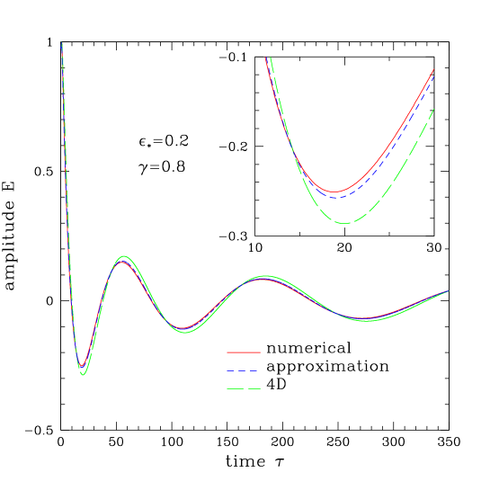
Figure 1: Numerical solution of GW on brane (solid), together with the 4-dimensional GW (long-dashed) and the result from the low-energy approximation (short-dashed, see Sec.4). The upper right window is the zoom-up of the solutions in the range $10<\tau<30$.

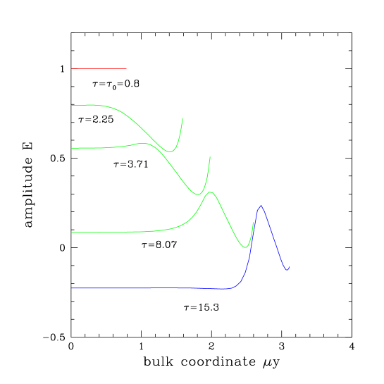
Figure 2: Snapshot of the waveform as function of the bulk coordinate $y$ in the case with the parameters $(\epsilon_{*},\gamma)=(0.2,0.8)$.

In Fig.1, the resultant waveform on the brane is depicted as function of time in the case with $\epsilon_{*}=0.2$, $\gamma=0.8$ and $N=64$. Apart from the overall damping $1/a_{0}(t)$ due to the cosmological expansion, the amplitude of the numerical solution on the brane (solid) becomes smaller than that of the solution in the four-dimensional theory (long-dashed). This result simply reflects the fact that the localization of gravity is not fulfilled in presence of the $\rho^{2}$-term (see Eq.(4)) and the GW can easily escape from the brane to the bulk.

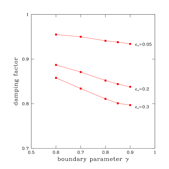
Figure 3: Damping factor of the GW amplitude on brane as function of boundary parameter $\gamma$

Fig.2 shows the snapshots of the waveform plotted as function of the original coordinate $y$. In the low-energy limit ($\rho/\lambda\ll 1$) of the present case, the equation (10) becomes separable and the analytic solution can be obtained as $E(\tau,y)=u(y)\phi(\tau)$. The mode function for the bulk coordinate $u(y)$ is given by

$$u_{0}(y)=\text{constant},$$ (13)

for the zero-mode and

$$u_{m}(y)=e^{2\mu y}H^{(1)}_{2}\left(\frac{m}{\mu}e^{\mu y}\right),$$ (14)

for the KK-mode with the effective mass $m$. The function $H^{(1)}_{2}(z)$ denotes the Hankel function for the second kind. We attempted to approximate the wave form of the numerical result by the superposition of the mode funcitons (13) and (14). If we set the mass of the KK-mode to the Hubble parameter at the horizon crossing time, the mode functions roughly reproduce the waveform of the numerical result, although the agreement is at a qualitative level. It is clear from Figs. 1 and 2 that the created KK-modes is rather light, consistent with our numerical set-up with $\epsilon_{*}\lesssim 1$, however, to obtain the KK-mode spectrum, a more quantitative analysis is needed.

The introduction of the regulator brane in the bulk is certainly not a proper way to treat the boundary condition in the bulk. The regulator brane may eventually affect the physical brane located at $y=0$. As shown in Fig.1, however, the excitation of the massive KK-modes becomes significant only at the horizon crossing time. The modification of the amplitude is almost determined around the horizon crossing and we need not follow the evolution of the perturbations for a long time. Thus, if the regulator brane is located sufficiently far away from the physical brane, we expect that we can safely neglect the effect of the regulator brane. To confirm this, in Fig.3, we plot the damping factor, i.e., the ratio of the amplitude obtained from the numerical solution to that from the four-dimensional theory in the case of $\epsilon_{*}=0.05$, $0.2$ and $0.3$. The number of collocation points used here is $N=64$ except for the cases of the boundary parameters $\gamma=0.85$ and $0.9$ with $N=128$. Since the suppression of GW amplitude is effective only when the mode crosses the Hubble horizon, the damping factor evaluated at the end of the calculaiton is time-independent. The damping factor depends linearly on small $\epsilon_{*}$, and tends to converge for $\gamma\rightarrow 1$.

4 Result from low-energy expansion

In order to understand the behavior of the numerical results in previous section, we employ a low energy expansion scheme to solve the wave equation approximately. In this treatment, the term $\rho/\lambda$ in effective Friedmann equation (4) is assumed to be small. Thus, treating the dimensionless quantity $\epsilon=\rho/\lambda$ as small expansion parameter, we expand the tensor perturbation $E(\tau,y)$, the scale factor $a_{0}(\tau)$ and the Hubble parameter $H(\tau)$:

$$E(\tau,y) =E_{0}(\tau)+E_{1}(\tau,y)+E_{2}(\tau,y)+\cdots,$$ (15)

$$a_{0}(\tau)\equiv e^{\alpha(\tau)} =e^{\alpha_{0}(\tau)}(1+\alpha_{1}(\tau)+\cdots),$$ (16)

$$H(\tau) =H_{0}(\tau)+H_{1}(\tau)+\cdots,$$ (17)

where $E_{k}(\tau,y)$, $\alpha_{k}(\tau)$ and $H_{k}(\tau)$ are the functions of the order $\mathcal{O}(\epsilon^{k})$. Note further the fact that in the low energy approximation, the time-derivative of the lower-order quantities is comparable to the $y$-derivative of the higher-order ones [12]. This is because the time derivative is of the order of the Hubble parameter, while the $y$-derivative is of the order of the bulk scale $\mu$. Thus, we have:

$$\left(\frac{\dot{\alpha}}{\alpha^{\prime}}\right)^{2}\sim\mathcal{O}(\epsilon).$$ (18)

Keeping the relation (18) in mind, one can expand the wave equation (10) in terms of $\epsilon$ and find the higher-order solutions iteratively. Then, imposing boundary conditions, we derive an ordinary differential equations for $E_{0}(\tau)$ [13].

The derivation of the equation for $E_{0}(\tau)$ is straightforward but lengthly calculation. The final form of the equation up to the first order in $\epsilon$ is

$$\begin{split}\Box_{\tau}E_{0}&=\frac{9\epsilon_{*}(1+w)^{2}}{8}\left(1-2B(y_{0})\right)\Box^{2}_{\tau}E_{0}\\ &-\frac{\rho}{\lambda}\left\{(2+3w)-(3w+5)B(y_{0})\right\}\Box_{\tau}E_{0}\\ &+\left\{3\frac{H_{1}}{H_{0}}-\frac{3}{2}(5+3w)(1+w)\frac{\rho}{\lambda}\left(1-2B(y_{0})\right)\right\}H_{0}\dot{E}_{0}\\ &+\left\{-2\alpha_{1}-3(1+w)\frac{\rho}{\lambda}\left(1-2B(y_{0})\right)\right\}\left(\frac{k}{e^{\alpha_{0}}}\right)^{2}E_{0},\end{split}$$ (19)

in the case of the static boundary. Here, we defined the operator $\Box_{\tau}$ and the quantity $B$ as follows:

$$\Box_{\tau}E_{0}\equiv-\,\frac{\partial^{2}E_{0}}{\partial\tau^{2}}-3H_{0}\frac{\partial E_{0}}{\partial\tau}-\left(\frac{k}{e^{\alpha_{0}}}\right)^{2}E_{0},$$ (20)

$$B(y_{0})\equiv\frac{\mu y_{0}}{1-e^{-2\mu y_{0}}}.$$ (21)

The variable $y_{0}$ denotes the position of the boundary determined at an initial time $\tau=\tau_{0}$, i.e., $y_{0}=\gamma y_{c}(\tau_{0})$. If the regulator brane is moving, the equation contains the term proportional to $\dot{y}_{\rm reg}(t)$ and it becomes rather complicated. Note also that this approximation will break down if the regulator brane becomes far away from our brane:

$$e^{\mu y_{\rm reg}}>\rho/\lambda,$$ (22)

since the low energy approximation breaks down on the regulator brane.

In spite of the above limitations of this approximation, the numerical results for $E_{0}(\tau)$ quite well reproduces the full numerical simulation even in the case of the moving boundary (see short-dashed in Fig.1). Thus, at least in a qualitative level, we can use this approximation to understand the behavior of perturbations on the brane.

The effective equation (19) contains a higher derivative term $\Box_{\tau}^{2}E_{0}$ which describes the non-local effect caused by the propagation of the wave in the bulk. If we numerically solve the equation with this higher-derivative term, we find that the solution badly diverges in time. It might be caused by the truncation of infinite numbers of higher derivative terms at a finite order. Hence we neglect the $\Box_{\tau}^{2}E_{0}$ term when we solve the ordinary differential equation (19) numerically. The first terms in the coefficients of $H_{0}\dot{E}_{0}$ and $k^{2}e^{-2\alpha_{0}}E_{0}$ come from the modification of background Friedmann equation, that is, $\rho^{2}$-term in Eq. (4). The second terms arise from the non-separable nature of the metric (1), which can be deduced from the fact that they vanish if we take $w=-1$. These are the terms which excite KK-modes in the bulk and cause the dissipation of the perturbations on the brane.

In the long wavelength limit $k\to 0$, the zero-mode solution $E_{0}=$ const. is the solution for the effective equation (19). However, if the perturbation crosses the horizon, the zero-mode solution which satisfies $\Box_{\tau}E_{0}=0$ cannot be a solution. Then the KK-modes are inevitably excited. The effects of the non-standard cosmological expansion tend to enhance the amplitude of the perturbation compared to the four-dimensional theory. On the other hand, both the numerical results and the low energy approximation show that the amplitude of the perturbations decreases, which implies that the influence of the excitation of KK-modes overcomes the effects of the non-standard cosmological expansion. Therefore, the suppression of the amplitude of GWs can be understood as the consequence of the excitation of the KK-modes due to the non-separable nature of the bulk metric in the Gaussian normal coordinate defined with respect to the physical brane.

5 Summary and Discussion

In this letter, we have numerically investigated the evolution of GWs during the radiation dominated epoch in the Randall-Sundrum type single-brane model. Especially focusing on the behavior after the horizon-crossing time, we found that the amplitude of GWs on brane is suppressed compared to that of the four-dimensional theory. To interpret the numerical results, we also employ the low energy approximation and derive the effective wave equation on the brane (Eq.(19)). The solution of this equation reasonably agrees with numerical simulations and the suppression of GWs can be understood as a consequence of the excitation of KK-modes. Although the created KK-modes seem to be rather soft, the influence of the KK-modes on GWs overcomes the effect of the non-standard cosmological expansion arising from the $\rho^{2}$-term. The suppression of GWs becomes significant as increasing the energy scales $\epsilon_{*}$. Therefore, contrary to the four-dimensional prediction, the intensity of the stochastic GWB around the frequency $f\sim f_{\rm crit}$ tends to decrease as increasing the frequency, which might provide an important clue to probe the presence or the absence of extra-dimensions.

For more quantitative prediction for the spectrum of stochastic GWB, however, the present numerical analysis has several limitations. While the evolved amplitude of GWs is examined at the relatively low energy scales $\epsilon_{*}\lesssim 1$, corresponding to the low-frequency modes with $f\lesssim f_{\rm crit}$, the high-frequency GWs with $f\gtrsim f_{\rm crit}$ are expected to suffer from the high-energy effects more seriously. As pointed out by [14], the created KK-modes does not simply escape away from the brane to the bulk in the high-energy region $\epsilon_{*}\gtrsim 1$. They could be turned back to the brane by the curvature scattering of the anti-de Sitter bulk, leading to the significant enhancement or the modulation of the GWs on brane.

In order to investigate the degree of this effect precisely, the boundary condition imposed on the regulator brane might be inadequate. Instead of using the Neumann condition (12), a suitable choice of the boundary condition such as the non-reflecting boundary condition should be considered. Further, to impose a realistic boundary condition, the Poincaré coordinate, which covers the wider region of the anti-de Sitter spacetime than the Gaussian normal coordinate, would be crucial in our numerical calculation. The implementation of these technical points is straightforward and the analysis is now in progress. We will report the results in a separate paper[13].

References

- [1] L.Randall and R.Sundrum, A large mass hierarchy from a small extra dimension, Phys. Rev. Lett. 83 (1999) 3370–3373 [hep-ph/9905221].
- [2] L.Randall and R.Sundrum, An alternative to compactification, Phys. Rev. Lett. 83 (1999) 4690–4693 [hep-th/9906064].
- [3] P.Binétruy, C.Deffayet, U.Ellwanger and D.Langlois, Brane cosmological evolution in a bulk with cosmological constant, Phys. Lett. B477 (2000) 285–291 [hep-th/9910219].
- [4] D.Langlois, R.Maatens and D.Wands,Gravitational wave from inflation on the brane, Phys. Lett. B489 (2000) 259–267.
- [5] J.Chiaverini, S.J.Smullin, A.A.Geraci, D.M.Weld and A.Kapitulnik, New experimental constraints on Non-Newtonian Forces below m, Phys. Rev. Lett 90 (2003) 151101.
- [6] C.J.Hogan, Scales of the extra dimensions and their gravitational wave backgrounds, Phys. Rev. D62 (2000) 121302(R).
- [7] M.Maggiore, Gravitational wave experiments and early universe cosmology Phys. Rep. 331 (2000) 283–367.
- [8] D.S.Gorbunov,V.A.Rubakov and S.M.Sibiryakov, Gravity waves from inflating brane or mirrors moving in AdS5, J. High. Energy Phys. 10 (2001) 015.
- [9] T.Kobayashi,H.Kudoh and T.Tanaka, Primordial gravitational waves in inflationary braneworld, Phys. Rev. D68 (2002) 044025 [gr-qc/0305006].
- [10] C.Canuto, M.Y.Hussaini, A.Quarteroni and T.A.Zang, Spectral Methods in Fluid Dynamics, Springer Verlag (Berlin and New York), 1988.
- [11] S.Bonazzola, E.Gourgoulhon, J.-A. Marck, Spectral methods in general relativistic astrophysics, J. Comput. Appl. Math. 109(1999) 433.
- [12] K.Koyama, Radion and large scales anisotropies on the brane, Phys. Rev. D66 (2002) 084003; S.Kanno and J. Soda, Radion and Holographic Brane Gravity, Phys. Rev. D66 (2002) 083506 .
- [13] T.Hiramatsu, K.Koyama and A.Taruya (2003), in preparation.
- [14] D.Langlois and L.Sorbo, Bulk gravitons from a cosmological brane, hep-th/0306281.
- [15] R.Easther, D.Langlois, R.Maartens and D.Wands, Evolution of gravitational waves in Randall-Sundrum cosmology, hep-th/0308078