The Energy-Momentum Problem in General Relativity

Sibusiso S. Xulu

This work is dedicated to my mother, Thokozile Maria (ukaMdlalose), and to my sister, Nozipho, who were both called to rest while I was writing this thesis.

ACKNOWLEDGEMENTS

I wish to express my thanks to the following individuals and organizations for their valuable contribution towards the completion of my thesis.

• My supervisor, Dr K. S. Virbhadra, for his excellent guidance, constructive criticism, and encouragement. He devoted his valuable time to introduce me to this subject. Dr Virbhadra thank you very much for many stimulating discussions and, for believing in me against the odds. Your thorough supervision and care in my work helped me complete seven articles which were all accepted in international journals. Your contribution in this regards is unequalled. You are the best teacher I have ever met in my life. It was indeed a privilege to be your student. My thanks also goes to your family members for their understanding when I usurped your attention.

• My co-supervisor, Prof. T. A. Dube, for encouragement and assistance.

• Prof. G. F. R. Ellis for hospitality at the university of Cape Town.

• The NRF for financial support.

• The University of Zululand Research Committee for financial support.

• My wife, Ntombi, and children, Lungi, Khayo and Hla for patience and support.

• I am also thankful to the anonymous examiners for helpful comments and suggestions.

DECLARATION

This thesis represents research work carried out by the author and has not been submitted in any form to another university for a degree. All the sources I have used have been duly acknowledged in the text.

ABSTRACT

Energy-momentum is an important conserved quantity whose definition has been a focus of many investigations in general relativity. Unfortunately, there is still no generally accepted definition of energy and momentum in general relativity. Attempts aimed at finding a quantity for describing distribution of energy-momentum due to matter, non-gravitational and gravitational fields only resulted in various energy-momentum complexes (these are nontensorial under general coordinate transformations) whose physical meaning have been questioned. The problems associated with energy-momentum complexes resulted in some researchers even abandoning the concept of energy-momentum localization in favor of the alternative concept of quasi-localization. However, quasi-local masses have their inadequacies, while the remarkable work of Virbhadra and some others, and recent results of Cooperstock and Chang et al. have revived an interest in various energy-momentum complexes. Hence in this work we use energy-momentum complexes to obtain the energy distributions in various space-times.

We elaborate on the problem of energy localization in general relativity and use energy-momentum prescriptions of Einstein, Landau and Lifshitz, Papapetrou, Weinberg, and Møller to investigate energy distributions in various space-times. It is shown that several of these energy-momentum complexes give the same and acceptable results for a given space-time. This shows the importance of these energy-momentum complexes. Our results agree with Virbhadra’s conclusion that the Einstein’s energy-momentum complex is still the best tool for obtaining energy distribution in a given space-time. The Cooperstock hypothesis (that energy and momentum in a curved space-time are confined to the the regions of non-vanishing energy-momentum of matter and the non-gravitational field) is also supported.

Chapter 1 Introduction

The notions of energy-momentum together with conservation laws play a fundamental role in any physical theory. The importance of conservation of energy and momentum concepts was first clearly identified more than two centuries ago within the Newtonian mechanics of a closed system of mass points. In this case both the linear momentum and the sum of kinetic and potential energies (for conservative forces) are conserved. The connection between these conservation laws and their invariance under Galilei group was only detected around the year 1900 (see in Havas[30]). In continuum mechanics of elastic bodies the formulation of energy conservation laws necessitated the introduction of the concept of strain energy. Maxwell and Poynting had to introduce the concepts of electric and magnetic energy densities in classical electrodynamics to retain energy conservation. Einstein’s famous result of the special theory of relativity (SR) that mass is equivalent to energy is a consequence of the requirement that the law of conservation of energy and momentum should hold in all inertial frames. As a matter of fact, this process of introducing new forms of energy in order to retain conservation laws characterizes the whole development of physics. However, this practice involving the introduction of new kinds of energy ran into serious difficulties with the arrival of the general theory of relativity (GR). The main difficulty is with the expression defining the gravitational field energy part.

Now, after more than eighty years of the success story of the theory of General Relativity (this includes, amongst other things, verification of the deflection of light by the Sun, the perihelion advance of Mercury, the gravitational red shift of light, and discoveries of quasars, cosmic fireball radiation, pulsars, X-ray sources that might contain black holes, and the present interest in the imminent detection of gravitational waves), there is still no general agreement on the definition of energy, and more generally, of conserved quantities associated with the gravitational field. This dilemma in GR is highlighted in an important paper by Penrose[53] in the following way: “It is perhaps ironic that energy conservation …which now has found expression in the (covariant) equation

$$\nabla_{a}T^{ab}=0,$$ (1.1)

…should nevertheless have found no universally applicable formulation, within Einstein’s theory, incorporating the energy of gravity itself”. Indeed, Einstein’s search for his generally covariant field equations was not only guided by the principle of equivalence but also by conservation laws of energy-momentum. Conservation laws of energy-momentum played a major role in the development of Einstein and Grossmann’s so-called Entwurf theory[49]. Although the field equations of the Entwurf theory were only of limited covariance, the theory had all the essential features of Einstein’s final theory of GR. Einstein and Grossmann had considered the use of the Ricci tensor in deriving almost covariant field equations but had rejected these equations because of misconceptions which were based on Einstein’s earlier work on static gravitational fields (for details see in Norton [49]).

In his[23] derivation of the generally covariant gravitational field equations, Einstein formulated the energy-momentum conservation law in the form:

$$\frac{\partial}{\partial x^{i}}(\sqrt{-g}(T_{j}^{\ i}+t_{j}^{\ i}))=0.$$ (1.2)

With $T_{j}^{\ i}$ representing the stress energy density of matter, Einstein identified $t_{j}^{\ i}$ as representing the stress energy density of gravitation. Einstein noted that $t_{j}^{\ i}$ was not a tensor, but concluded that the above equations $(\ref{EMconEq})$ hold good in all coordinate systems since they were directly obtained from the principle of general relativity. The choice of a nontensorial quantity to describe the gravitational field energy immediately attracted some criticism. Levi-Civita not only attacked Einstein’s use of a pseudotensor quantity (which is only covariant under linear transformations) in describing the gravitational field energy, but also suggested an alternative gravitational energy tensor which required that Einstein’s field equations be also interpreted as conservation laws (for details see in Cattani and De Maria [11], and in Pauli [52] ). Both Schrödinger and Bauer came up with counter examples to Einstein’s choice of a nontensor. Schrödinger showed that by a suitable choice of a coordinate system the pseudotensor of a Schwarzschild solution vanishes everywhere outside the Schwarzschild radius. Bauer’s example illustrated that a mere introduction of polar coordinates instead of quasi-Cartesian coordinates into a system of inertia without matter present would create a nonvanishing energy density in space. By resorting to the equivalence principle and physical arguments, Einstein vigorously defended the use of his pseudotensor to represent gravitational field[11]. The problems associated with Einstein’s pseudotensor resulted in many alternative definitions of energy, momentum and angular momentum being proposed for a general relativistic system (see Aguirregabiria et al [1] and references therein).

The lack of a generally accepted definition of energy distribution in curved space-times has led to doubts regarding the idea of energy localization. The ambiguity in the localization of energy is not a new physics problem, peculiar to the theory of GR, but is also present in classical electrodynamics (Feynmann et al[25]. In GR there is a dispute with the importance of non-tensorial energy-momentum complexes whose physical interpretation has been questioned by a number of scientists, including Weyl, Pauli and Eddington (see in Chandrasekhar and Ferrari [15]). There are suspicions that, in a given space-time, different energy distributions would be obtained from different energy-momentum complexes. However, Virbhadra and co-workers investigated several examples of particular space-times (the Kerr-Newman, the Einstein-Rosen, and the Bonnor-Vaidya) and found that different energy-momentum complexes give the same energy distribution for a given space-time. Several energy-momentum complexes have been shown to coincide for any Kerr-Schild class metric [1]. In this thesis we are extending the work of Virbhadra and co-workers by considering further space-times in showing that the energy-momentum complexes are useful in obtaining meaningful energy distribution in a given geometry. In the rest of the chapter we give a brief review of both the theory of special relativity and general relativity so as to establish both the notation and terminology which will be used in the rest of our discussion. We also give a list of formulas needed in our later discussion.

1.1 Tensor equations

Einstein’s 1905 paper on the special theory of relativity which demanded a complete change of attitude towards space and time prompted Minkowski to declare with great elegance, in his famous 1908 speech, that “Henceforth space by itself and time by itself, are doomed to fade away into mere shadows, and only a kind of union of the two will preserve an independent reality.” The importance of this is supported by the simplicity obtained by formulating the physical laws in four-dimensional space-time. In special relativity this simplicity is obtained by using the Minkowski space-time:

$$ds^{2}=\eta_{pq}dx^{p}dx^{q},$$ (1.3)

where $\eta_{pq}=diag(1,-,1,-1,-1)$. (Throughout we use the convention that summation occurs over dummy indices, Latin indices take values from 0 to 3 and Greek indices values from 1 to 3, and take $G=1$ and $c=1$ units. The comma and semi-colon indicate ordinary and covariant differentiation, respectively.) The presence of gravitation necessitates a generalization of the Minkowski space-time into the four dimensional Riemannian space-time:

$$ds^{2}=g_{pq}dx^{p}dx^{q},$$ (1.4)

where $g_{ab}=g_{ab}(x^{i})$ is the metric tensor, symmetric in its indices, which characterizes the space-time completely. In the rest of this section we present important formulas/properties in Riemannian spaces required for our later work.

A contravariant metric tensor $g^{ab}$ is defined as

$$g^{ab}=\frac{\Delta^{ab}}{g},$$ (1.5)

where $\Delta^{ab}$ is a cofactor of $g_{ab}$, while $g=\det(g_{pq})$. From this definition it is obvious that $g^{ab}$ is also symmetric in its indices and that:

$$g_{bp}g^{pa}=\delta_{b}^{a}.$$ (1.6)

The relationship:

$$dg=gg^{pq}\,dg_{pq}=-gg_{pq}\,dg^{pq}$$ (1.7)

follows from $(\ref{teq3})$ and $(\ref{teq4})$. The metric tensor $g_{ab}$ transforms under coordinates transformation $x^{a}\rightarrow x^{a^{\prime}}$ as:

$$g_{a^{\prime}b^{\prime}}=\frac{\partial x^{p}}{\partial x^{a^{\prime}}}\frac{\partial x^{q}}{\partial x^{b^{\prime}}}g_{pq},$$ (1.8)

whereas its determinant $g$ transforms under coordinates transformation as a scalar density of weight $+2$:

$$g^{\prime}=\left|\frac{\partial x}{\partial x^{{}^{\prime}}}\right|^{2}g,$$ (1.9)

where $\left|\frac{\partial x}{\partial x^{{}^{\prime}}}\right|$ is the Jacobian of the coordinates transformation. In general, a quantity which transforms like:

$$\Re_{b^{\prime}...}^{a^{\prime}...}=\left|\frac{\partial x}{\partial x^{{}^{\prime}}}\right|^{W}\frac{\partial x^{a^{\prime}}}{\partial x^{p}}...\frac{\partial x^{q}}{\partial x^{b^{\prime}}}...\Re_{q...}^{p...}$$ (1.10)

is called a tensor density of weight $W$. Using $dx^{a^{\prime}}=\frac{\partial x^{a^{\prime}}}{\partial x^{p}}dx^{p}$ and $(\ref{teq7})$ we can deduce that $\left(-g\right)^{-w/2}\,\Re_{b^{\prime}...}^{a^{\prime}...}$  is an ordinary tensor if $\Re_{b^{\prime}...}^{a^{\prime}...}$ is a tensor density of weight $W$. Thus for a four-dimensional volume element $d^{4}x$ the quantity $\sqrt{-g}\,d^{4}x$ is an invariant. An important tensor density of weight $+1$, called the Levi-Civita contravariant tensor density, is defined as:

$$\varepsilon^{abcd}=\left\{\begin{array}[]{clcr}&+1,\text{ if }abcd\text{ is an even permutation of }0123\\ &-1,\text{ if }abcd\text{ is an odd permutation of }0123\\ &\ \ 0,\text{ otherwise.}\end{array}\right.$$ (1.11)

$\varepsilon^{abcd}$ is totally anti-symmetric and has the useful property that its components are the same in all coordinate systems. Any totally skew-symmetric tensor of order $4$ is proportional to this tensorial quantity. The covariant component Levi-Civita tensor density $\varepsilon_{abcd}$ may then be defined in terms of the contravariant component by the usual lowering of indices as:

$$\varepsilon_{abcd}=(-g)g_{ap}g_{bq}g_{cr}g_{ds}\varepsilon^{pqrs}.$$ (1.12)

The tensor density $\varepsilon_{abcd}$ will be of weight $-1$. The above tensor densities can also be used to define the following totally antisymmetric unit tensors of rank four. The contravariant tensor $\epsilon^{abcd}$ is defined as:

$$\epsilon^{abcd}=\frac{\varepsilon^{abcd}}{\sqrt{-g}},$$ (1.13)

while the corresponding covariant tensor is defined by:

$$\epsilon_{abcd}=\sqrt{-g}\,\varepsilon_{abcd}.$$ (1.14)

If $A_{ij}$ is an antisymmetric tensor, then using $\varepsilon^{abcd}$ and $\epsilon^{abcd}$ we may define:

$${}^{\ast}{\mathcal{A}}^{ij}=\frac{1}{2}\varepsilon^{ijpq}A_{pq},$$ (1.15)

and

$${}^{\ast}{A}^{ij}=\frac{1}{2}\epsilon^{ijpq}A_{pq},$$ (1.16)

where ${}^{\ast}{\mathcal{A}}^{ij}$ and ${}^{\ast}{A}^{ij}$ are said to be a dual pseudotensor and a dual tensor respectively to $A_{ij}$. Using $A^{ij}$ both ${}^{\ast}{\mathcal{A}}_{ij}$ and ${}^{\ast}{A}_{ij}$ may be defined in a similar way in terms of $\varepsilon_{abcd}$ and $\epsilon_{abcd}$ respectively.

The motion of an infinitesimally small particle moving in a gravitational field is described by the geodesic equation:

$$\frac{d^{2}x^{a}}{ds^{2}}+\Gamma_{pq}^{a}\frac{dx^{p}}{ds}\frac{dx^{q}}{ds}=0,$$ (1.17)

which can be deduced from $(\ref{teq2})$ by taking the deviation of the action integral:

$$I=\int ds,$$ (1.18)

where $\Gamma_{bc}^{a}$ are the Christoffel symbols of the second kind given by:

$$\Gamma_{bc}^{a}=\frac{1}{2}g^{ap}\left(g_{bp,c}+g_{cp,b}-g_{bc,p}\right).$$ (1.19)

By contracting the pair of indices $a$ and $c$ in the above $(\ref{teq19})$ we obtain

$$\Gamma_{bp}^{p}=\frac{1}{2}g^{pq}g_{pq,b},$$ (1.20)

and combining this result with that of Eqn $(\ref{teq5})$ we deduce that:

$$\Gamma_{bp}^{p}=\frac{1}{2g}\frac{\partial g}{\partial x^{b}}=\frac{\partial\ln\sqrt{-g}}{\partial x^{b}}.$$ (1.21)

The identity that the $g^{ab}_{~{}~{};c}=0$ gives us the following relationship:

$$g^{ab}_{~{}~{},c}=-g^{ap}\Gamma_{pc}^{b}-g^{pb}\Gamma_{pc}^{a}.$$ (1.22)

¿From the definition of covariant differentiation we may deduce the following useful relation:

$$A_{a;b}-A_{b;a}=A_{a,b}-A_{b,a}.$$ (1.23)

The Riemann curvature tensor is defined using the above Christoffel symbols as:

$$R_{~{}bcd}^{a}=\Gamma_{bd,c}^{a}-\Gamma_{bc,d}^{a}+\Gamma_{pc}^{a}\Gamma_{bd}^{p}-\Gamma_{pd}^{a}\Gamma_{bc}^{p},$$ (1.24)

which vanishes if and only if the space-time under consideration is flat. In geodesic coordinate system (i.e. coordinate system where components of Christoffel symbols vanish at the pole of this special coordinate system) the Riemann curvature tensor takes the simpler form:

$$R_{~{}bcd}^{a}=\Gamma_{bd,c}^{a}-\Gamma_{bc,d}^{a}.$$ (1.25)

By lowering the upper index of the Riemann tensor $(\ref{teq20})$ to $R_{abcd}=g_{ap}R_{~{}bcd}^{p}$ then its symmetry properties become easy to study. $R_{abcd}$ is anti-symmetric in each of the pair of indices $ab$ and $cd$, and is symmetric under the exchange of these pairs of indices with each other. The cyclic sum of components of $R_{abcd}$ formed by a permutation of any three indices is equal to zero. Several important tensors may be constructed using this tensor. By contraction of the Riemann curvature tensor we obtain the Ricci tensor defined by

$$R_{ab} = R_{~{}apb}^{p}=g^{pq}R_{paqb}$$ (1.26)

$$= \Gamma_{ab,p}^{p}-\Gamma_{ap,b}^{p}+\Gamma_{ab}^{q}\Gamma_{pq}^{p}-\Gamma_{ap}^{q}\Gamma_{bq}^{p},$$ (1.27)

which is symmetric in its indices. The Ricci scalar curvature is:

$$R=R_{~{}p}^{p}=g^{pq}R_{pq}.$$ (1.28)

The Einstein tensor is defined in terms of the Ricci tensor as:

$$G_{ab}=R_{ab}-\frac{1}{2}g_{ab}\,R.$$ (1.29)

Similarly the above Einstein’s tensor is symmetric in its indices. The traceless Weyl conformal tensor $C_{abcd}$ is again defined in terms of Riemann tensor as:

$$C_{abcd} = R_{abcd}-\frac{1}{2}\left(g_{ac}R_{bd}-g_{ad}R_{bc}-g_{bc}R_{ad}+g_{bd}R_{ac}\right)$$ (1.30)

$$+\frac{1}{6}\left(g_{ac}g_{bd}-g_{ad}g_{bc}\right).$$

The symmetry properties of $C_{abcd}$ are similar to those of the Riemann curvature tensor. The importance of the Weyl tensor is in its invariance under conformal mapping of two Riemannian spaces. The Bianchi identities are given by

$$\nabla_{a}R_{~{}qbc}^{p}+\nabla_{b}R_{~{}qca}^{p}+\nabla_{c}R_{~{}qab}^{p}=0.$$ (1.31)

These identities take a much simpler form if expressed in terms of the dual ${}^{\ast}R_{pqrs}$ to the Riemann tensor $R_{abcd}$

$$\nabla^{p}\,{}^{\ast}R_{abcp}=0.$$ (1.32)

By using the fact that the covariant derivatives of the metric tensor vanishes and contracting the Bianchi identities 1.31 we get the following important relationship:

$$\nabla_{p}G^{~{}p}_{a}=0,$$ (1.33)

or the following equivalent identity:

$$\nabla_{p}R^{~{}p}_{a}=\frac{1}{2}\frac{\partial R}{\partial x^{a}}.$$ (1.34)

1.2 Special relativity

The idea of relativity can be traced back to Galileo who was the first to state clearly the concept of relative motion. His example of a boat which is in uniform motion illustrates that no experiment performed in a sealed cabin can be able to detect motion. According to the Galilean principle of relativity all laws of mechanics are the same in all inertial reference frames. The space $x^{\alpha}\rightarrow x^{\alpha\prime}$ and time $t\rightarrow t^{\prime}$ coordinates transformations between any two inertial frames, K and K’, may be written as:

$$x^{\alpha\prime} = M^{\alpha}_{~{}\beta}\,x^{\beta}+v^{\alpha}\,t+d^{\alpha},$$

$$t^{\prime} = t+t_{0},$$ (1.35)

where constants $M^{\alpha}_{~{}\beta}$, $v^{\alpha}$, $d^{\alpha}$ and $t_{0}$ respectively represent rotations, uniform motion, space and time translations of origins of reference systems. The so-called Galilean transformations $(\ref{GalTrEq})$ form a ten-parameters group of, namely three rotation Euler angles in the orthogonal matrix $M$, three components in each of $v^{\alpha}$ and $d^{\alpha}$, and lastly the constant $t_{0}$. Newton’s fundamental equations of classical mechanics, based on the concepts of absolute space and absolute time, are invariant in all inertial reference frames under Galilean coordinate transformations. If we consider three inertial coordinates frames $K_{1}$, $K_{2}$, and $K_{3}$, then using the group property of Galilean transformations we obtain the following velocity addition law:

$$v_{\mathbf{13}}^{\alpha}=v_{\mathbf{12}}^{\alpha}+v_{\mathbf{23}}^{\alpha},$$ (1.36)

where $v_{\mathbf{ab}}^{\alpha}$ is velocity of $K_{b}$ relative to $K_{a}$. This velocity addition law (1.36) is valid in Newtonian mechanics. However, Maxwell’s theory of classical electrodynamics implied that light travels in vacuum at a constant speed $c$. Obviously, according to Galilean velocity addition law light could not have the same speed $c$ with respect to arbitrary inertial frames. One can also verify that the wave equation for electrodynamics in free space is not invariant under Galilean transformations. The fact that Newton’s equations of mechanics are invariant under Galilean transformations while the Maxwell equations are not, leads one to enquire whether it is possible to find some principle of relativity which holds for both mechanics and electrodynamics, but where

• Newton’s laws of mechanics are not correct, or

• Maxwell’s laws of electrodynamics are not correct?

Experimental evidence indicating deviations from either the Newtonian or Maxwellian theory is required in order to decide whether the laws of mechanics or electrodynamics need to be reformulated.

The famous Michelson-Morley experiment showed that the velocity of light is the same for light travelling along the direction of the earth’s orbital motion and transverse to it. Numerous attempts were made to explain the Michelson-Morley null result of the earth’s motion through ether. Fitzgerald and Lorentz independently suggested that material bodies contract in the direction of the their motion by a factor $\sqrt{1-v^{2}/c^{2}}$. Lorentz explained the contraction hypothesis in terms of an electromagnetic model of matter, and introduced length transformation and the concept of a ‘local time’. Poincaré called for the development of a new mechanics to replace the Newtonian mechanics (see in Schröder [57]). He showed that the Maxwell equations in vacuo are invariant under the Lorentz transformations. He further showed that Lorentz transformations form a group[57]. The inhomogeneous Lorentz space-time $x^{a}\rightarrow x^{a^{\prime}}$ coordinate transformations , also called the Poincaré group, are given by:

$$x^{a^{\prime}}=\Lambda_{p}^{a}\,x^{p}+d^{a},$$ (1.37)

where constants $d^{a}$ denote space and time translations, while $\Lambda_{b}^{a}$ represent rotations and uniform motion of the origins of inertial frames. The matrix $\Lambda$ must satisfy the following condition:

$$\Lambda_{a}^{p\,}\Lambda_{b}^{q}\eta_{pq}=\eta_{ab},$$ (1.38)

with

$$\eta_{pq}=\eta^{pq}=diag(1,-1,-1,-1).$$ (1.39)

The so-called proper Lorentz group is obtained by imposing the following additional conditions:

$$\Lambda_{0}^{0\,}\geq 1,\mbox{ }det(\Lambda)=1.$$ (1.40)

If there are no translations, i.e. $d^{a}=0$, we get the homogeneous Lorentz group.

The incompatibility of mechanics with electrodynamics was finally resolved by Albert Einstein who proposed a replacement of the Galilean transformations by the Lorentz transformations. Einstein’s theory of special relativity (STR) is based on the following postulates:

• The principle of relativity. The laws of physics are the same in all inertial reference frames.

• The constancy of the speed of light. The speed of light in vacuum is the same for all inertial observers irrespective of the motion of the source.

Following Einstein’s approach, then the above Lorentz transformations $(\ref{LorTrEq})$ become a consequence of the constancy of the speed of light. As already mentioned, in special relativity physical laws are formulated in four-dimensional Minkowski space-time. The interval $I_{AB}$ between two events $A$ and $B$, with coordinates $\left(t_{A},x_{A},y_{A},z_{A}\right)$ and $\left(t_{B},x_{B},y_{B},z_{B}\right)$, given by:

$$I_{AB}=(x_{A}^{0}-x_{B}^{0})^{2}-(x_{A}^{1}-x_{B}^{1})^{2}-(x_{A}^{2}-x_{B}^{2})^{2}-(x_{A}^{3}-x_{B}^{3})^{2},$$ (1.41)

Figure 1.1: $t>0$ and $t<0$ represent forward and backward null cones, respectively.

is an invariant under Lorentz transformations. (Note that $x^{0}=ct$ and that $c=1$). $I_{AB}$ is said to be timelike if $I_{AB}>0,$ spacelike if $I_{AB}<0,$ and lightlike or null if $I_{AB}=0$. For a timelike interval of two events, it is possible to do a Lorentz transformation to an inertial frame where the two events occur at the same point, but there is no inertial frame where they occur at the same time. Therefore, for any two timelike events if $x_{A}^{0}>x_{B}^{0}$ then $A$ is said to be in the absolute future of $B$, while if $x_{A}^{0}<x_{B}^{0}$ then $A$ is said to be in the absolute past of $B$. In a spacelike interval for any two events it is always possible to do a Lorentz transformation to an inertial frame where the two events occur at the same time, but it is impossible to choose a frame where they occur at the same point.

In Minkowski space-time the motion of a mass point is described by the world line $x^{i}=x^{i}(\lambda)$, where $\lambda$ is parameter determining motion. Now, by observing that the proper time $d\tau$, given by:

$$d\tau^{2}=\eta_{pq}\,dx^{p}\,dx^{q},$$ (1.42)

is an invariant under Lorentz coordinate transformations,the velocity four-vector $u^{i}$ and the acceleration four-vector are defined with respect to the proper time as:

$$u^{i}=\frac{dx^{i}}{d\tau},$$ (1.43)

and

$$\dot{u^{i}}=\frac{du^{i}}{d\tau}.$$ (1.44)

Newton’s equations, in their original form, are no longer invariant under the Lorentz transformations, but using the above definitions the four-vector relativistic force of Newton’s second law takes the form:

$$f^{a}=m\frac{d^{2}x^{a}}{d\tau^{2}},$$ (1.45)

or in terms of the relativistic energy-momentum:

$$p^{a}=m\frac{dx^{a}}{d\tau},$$ (1.46)

the relativistic force may be expressed by:

$$f^{a}=\frac{dp^{a}}{d\tau},$$ (1.47)

where $p^{a}$ is also a four-vector. $f^{a}$ is commonly referred to as the Minkowski force. The spatial components of the four-vector Minkowski force $f^{a}=(f^{0},\mathbf{f})$ are related to the Newtonian force $\mathbf{F}$ by the following:

$$\mathbf{f}=\gamma\mathbf{F},$$ (1.48)

and its time component is given by

$$f^{0}=\gamma\mathbf{F\cdot v},$$ (1.49)

where ${\bf v:=}\frac{d{\bf x}}{dt}$ and $\gamma:=\left(1-{\bf v}^{2}\right)^{-1/2}$. The time component of $p^{a}$ is the energy:

$$p^{0}=E=m\gamma,$$ (1.50)

and the space components $p^{\alpha}$ form the momentum vector:

$${\bf p}=m\gamma{\bf v}.$$ (1.51)

Thus the four-vector $p^{a}$ is called the energy-momentum vector. This energy-momentum vector is conserved in all inertial reference frames related by Lorentz transformations. For a particle with rest mass $m>0$ we have that:

$$p_{a}p^{a}=m^{2},$$ (1.52)

which gives the following equation connecting the energy and momentum:

$$E^{2}-\mathbf{p}^{2}=m^{2}.$$ (1.54)

Taking the ratio of equations $(\ref{STReq11})$ and $(\ref{STReq12})$ we get the following useful expression:

$$\frac{{\bf p}}{E}={\bf v}.$$ (1.55)

The Maxwell equations of electrodynamics in vacuum:

$$\nabla\cdot{\bf E} = 4\pi\rho,$$ (1.56)

$$\nabla\times{\bf B}-\frac{\partial{\bf E}}{\partial t} = 4\pi{\bf j},$$ (1.57)

$$\nabla\cdot{\bf B} = 0,$$ (1.58)

$$\nabla\times{\bf E}+\frac{\partial{\bf B}}{\partial t} = {\bf 0},$$ (1.59)

where $\mathbf{E}$ and $\mathbf{B}$ are respectively the electric and magnetic fields, are invariant under Lorentz coordinate transformations. This may be illustrated by expressing the above equations in a covariant form in terms of an anti-symmetric electromagnetic field tensor $F_{ab}$ which may be defined as:

$$F^{ab}:=\left[\begin{array}[]{cccc}0&E_{x}&E_{y}&E_{z}\\ -E_{x}&0&B_{z}&-B_{y}\\ -E_{y}&-B_{z}&0&B_{x}\\ -E_{z}&B_{y}&-B_{x}&0\end{array}\right]$$ (1.60)

Then using Eq. $(\ref{MxlTeq})$ the Maxwell equations $(\ref{MxlEq1},\ref{MxlEq2},\ref{MxlEq3},\ref{MxlEq4})$ may now be reduced to the following two tensorial equations:

$$\frac{\partial F^{ab}}{\partial x^{b}} = -4\pi j^{a},$$ (1.61)

$$\frac{\partial^{*}F^{ab}}{\partial x^{b}} = 0,$$ (1.62)

where ${}^{*}F^{ab}$ is the dual tensor of $F^{ab}$, $j^{a}$ is the four-vector of current density with the components:

$$j^{a}=(\rho,\mathbf{\rho\mathbf{v}}),$$ (1.63)

with $\rho$ being the charge density, and $\mathbf{v}$ the velocity of charge. The equation of continuity for the current density:

$$\frac{\partial j^{a}}{\partial x^{a}}=0,$$ (1.64)

now follows directly from Eq.$(\ref{MxlCovEq1})$. Eq.$(\ref{MxlCovEq2})$ can also be expressed as:

$$\frac{\partial}{\partial x^{a}}F_{bc}+\frac{\partial}{\partial x^{b}}F_{ca}+\frac{\partial}{\partial x^{c}}F_{ab}=0.$$ (1.65)

The relativistic electromagnetic force on a charged particle may be written in terms of the Maxwell tensor as:

$$f^{a}=eF_{~{}p}^{a}\frac{dx^{p}}{d\tau},$$ (1.66)

where $e$ is the charge parameter.

1.3 The Energy-momentum tensor

The energy-momentum of the electromagnetic field in free-space may be obtained by considering the action integral formed with the Lagrangian density:

$$\mathcal{L}_{\mathbf{F}}=-\frac{1}{16\pi}F_{ab}F^{ab},$$ (1.67)

which gives the following contravariant components of the energy-momentum tensor:

$$T^{ab}=-\frac{1}{4\pi}\frac{\partial A^{p}}{\partial x_{a}}F^{b}_{~{}p}+\frac{1}{16\pi}\eta^{ab}F_{pq}F^{pq},$$ (1.68)

where $A^{a}$ is the four-vector of the potentials. This tensor is then symmetrized by adding the quantity $\frac{1}{4\pi}\frac{\partial A^{a}}{\partial x_{p}}F^{b}_{~{}p}$ and using the fact that in the absence of charges then Eq.$(\ref{MxlCovEq1})$ takes the form:

$$\frac{\partial F^{ab}}{\partial x^{b}}=0,$$

which finally leads to the following symmetric energy-momentum tensor expression:

$$T^{ab}=\frac{1}{4\pi}(-F^{ap}F^{b}_{~{}p}+\frac{1}{4}\eta^{ab}F_{pq}F^{pq}).$$ (1.69)

This tensor $(\ref{EMTeq1b})$ is gauge invariant and has a vanishing trace, $T^{a}_{~{}a}=0$ and most importantly it satisfies:

$$T^{a}_{~{}b,a}=0.$$ (1.70)

The fact that $T^{a}_{~{}b}$ is divergeless indicates that the four-vector:

$$P^{a}=\int_{\sigma}T^{ab}dS_{b},$$ (1.71)

is conserved, where $\sigma$ is an arbitrary spacelike hypersurface. Now since the integral $(\ref{EMVeq1})$ is independent of the hypersurface $\sigma$, choosing the hypersurface $x^{0}=constant$, i.e. a three-dimensional space, then:

$$P^{a}=\int T^{a0}d^{3}x,$$ (1.72)

may be identified as the total energy-momentum four-vector of the field. The angular momentum tensor:

$$M^{abc}=T^{ab}x^{c}-T^{ac}x^{b},$$ (1.73)

defined in terms of $T^{ab}$, satisfies:

$$M^{abc}_{~{}~{}~{},a}=0,$$

which shows that the total field angular momentum

$$J^{ab}=\int M^{0ab}d^{3}x,$$ (1.74)

is also conserved.

The energy-momentum tensor $(\ref{EMTeq1b})$ is only defined for charge-free fields. In the presence of charged objects then we should not only consider contributions from the electromagnetic field but also from the charged objects themselves. Thus the energy-momentum tensor of field together with charges is:

$$T^{ab}=T^{ab}_{\mathbf{F}}+T^{ab}_{\mathbf{M}},$$

where subscripts $\mathbf{F}$ and $\mathbf{M}$ indicate field and matter contributions, respectively. Now we should have that:

$$\frac{\partial}{\partial x^{a}}(T^{ab}_{\mathbf{F}}+T^{ab}_{\mathbf{M}})=0,$$ (1.75)

where $T^{ab}_{\mathbf{F}}$ is given by $(\ref{EMTeq1b})$. Now differentiating equation $(\ref{EMTeq1b})$ and simplifying, and making use of the inhomogeneous Maxwell equations $(\ref{MxlCovEq1})$ together with $(\ref{MxlCovEq2})$ we get

$$\frac{\partial}{\partial x^{a}}T^{ab}_{\mathbf{F}}=-F^{bp}j_{p}.$$ (1.76)

For a system of non-interacting particles, the energy momentum tensor is given by

$$T^{ab}_{\mathbf{M}}=\mu u^{a}u^{b}\frac{ds}{dt},$$ (1.77)

where $\mu$ defined as:

$$\mu=\mathrel{\mathop{\sum}\limits_{\mbox{n}}}m_{\mbox{n}}\delta(\mathbf{r-r_{\mbox{n}}}),$$ (1.78)

may be termed the ‘mass density’ since it indicates the continuous mass distribution in space. Noting that mass should be conserved for non-interacting particles, we have:

$$\frac{\partial}{\partial x^{a}}(\mu\frac{ds}{dt})=0,$$ (1.79)

and making use of Eq. $(\ref{EMFeq})$ we get

$$\frac{\partial}{\partial x^{a}}T^{ab}_{\mathbf{M}}=F^{bp}j_{p}.$$ (1.80)

Hence equations $(\ref{EFeq})$ and $(\ref{EMMeq})$ show that equation $(\ref{EMconsEq})$ is indeed satisfied. From this discussion it is clear that electromagnetic fields are determined by the motion of charges, while on the other hand the motion of charges is determined by the fields, i.e. the two systems are interdependent on each other.

1.4 The Einstein field equations

In this section we give a derivation of the Einstein field equations for gravitation from a variational principle, but before that we give both the equivalence principle and the principle of general covariance which guided Einstein in his search for equations of gravitation. The equivalence principle is based on the equality of the gravitational mass and the inertial mass. Several experiments have been performed, starting from Galileo, Newton, Bessel, Eötvös, and many others, to investigate whether or not there is a difference between the gravitational and inertial masses of objects. The Eötvös torsion balance experiment showed with a high degree of accuracy the equality of the inertial and gravitational mass. The principle of equivalence may be formulated as[75]: At every spacetime point in an arbitrary gravitational field it is possible to choose a “locally inertial coordinate system” such that, within a sufficiently small region of the point in question, the laws of nature take the same form as in a Minkowski spacetime , i.e. the gravitational field may be eliminated locally by the use of a freely falling coordinate system.

The principle of general covariance may be stated in one of the following forms[9], namely

1. All coordinate systems are equally good for stating the laws of physics.

2. The equations that describe the laws of physics should have tensorial forms and be expressed in four-dimensional Riemannian spacetime.

3. The equations describing the laws of physics should have the same form in all coordinate systems.

One considers the Ricci scalar curvature $\,R\,=g^{pq}R_{pq}$ as our Lagrangian to derive the Einstein field equations. The action integral for the gravitational field is then given by:

$$\int\sqrt{-g}\,R\,d^{4}x,$$ (1.81)

where the integration is taken over all space and over the time component $x^{0}$ between two given values. To encompass non-gravitational fields in a physical system we include another Lagrangian $L_{F}$ for all the other fields, so that our expression for the action integral is given by:

$$I=\int\sqrt{-g}\,(R-2\,\kappa\,L_{F})\,d^{4}x,$$ (1.82)

where $\kappa$ is Einstein’s gravitational constant. We require that the variation of the above be equal to zero,

$$\delta I=0.$$ (1.83)

The variation of the first part of I is:

$$\delta\int\sqrt{-g}\,R\,d^{4}x=\int\sqrt{-g}\,g^{pq}\,\delta R_{pq}\,d^{4}x+\int R_{pq}\,\delta\left(\sqrt{-g}\,g^{pq}\right)\,d^{4}x.$$ (1.84)

By simplifying and applying Gauss theorem it can then be shown that:

$$\int\sqrt{-g}\,g^{pq}\,\delta R_{pq}\,d^{4}x=0.$$ (1.85)

Therefore

$$\delta\int\sqrt{-g}\,R\,d^{4}x = \int\sqrt{-g}\,R_{pq}\,\delta g^{pq}\,d^{4}x+\int R\,\delta\sqrt{-g}^{pq}\,d^{4}x$$ (1.86)

$$= \int\sqrt{-g}\,\left(R_{pq}-\frac{1}{2}g_{pg}\,R\,\right)\delta g^{pq}\,d^{4}x.$$

Now the second part of action integral:

$$\delta\int\sqrt{-g}\,L_{F}\,d^{4}x = \int\left[\frac{\partial\left(\sqrt{-g}\,L_{F}\right)}{\partial g^{pq}}\delta g^{pq}-\frac{\partial\left(\sqrt{-g}\,L_{F}\right)}{\partial g_{,a}^{pq}}\delta g_{,a}^{pq}\right]\,d^{4}x$$ (1.87)

$$= \frac{1}{2}\int\sqrt{-g}\,T_{pq}\,\delta g^{pq}\,d^{4}x,$$

where $\,T_{pq}$ is the energy-momentum tensor defined as:

$$\,T_{pq}=\frac{2}{\sqrt{-g}}\left[\frac{\partial\left(\sqrt{-g}\,L_{F}\right)}{\partial g^{pq}}-\frac{\partial}{\partial x^{a}}\left\{\frac{\partial\left(\sqrt{-g}\,L_{F}\right)}{\partial g_{,a}^{pq}}\right\}\right].$$ (1.88)

Now using results of $(\ref{Efeq6})$ and $(\ref{Efeq7})$ then the variation of $(\ref{Efeq2})$ is:

$$\delta I=\int\sqrt{-g}\,\left(R_{pq}-\frac{1}{2}g_{pg}\,R-\kappa\,T_{pq}\,\right)\delta g^{pq}\,d^{4}x,$$ (1.89)

and since $\delta g^{pq}$ is an arbitrary variation this gives us the Einstein field equations:

$$R_{pq}-\frac{1}{2}g_{pg}\,R=\kappa\,T_{pq}.$$ (1.90)

1.5 Maxwell equations in presence of gravitation

In the absence of gravitation, the Maxwell field equations are expressed by $(\ref{MxlCovEq1})$ and $(\ref{MxlCovEq2})$. However, in the presence of gravitation these equations are generalized by the following equations by replacing partial derivatives to covariant derivatives. Therefore one has now

$$F_{ab;c}+F_{bc;a}+F_{ca;b}=0,$$ (1.91)

and

$$F^{ap}_{~{}~{};p}=-4\pi j^{a}.$$ (1.92)

The above two equations can easily be expressed as

$$F_{ab,c}+F_{bc,a}+F_{ca,b}=0,$$ (1.93)

and

$$\frac{\partial}{\partial x^{p}}\left[\sqrt{-g}F^{ap}\right]=-4\pi\sqrt{-g}j^{a}.$$ (1.94)

The continuity equation $(\ref{ContEq})$ now takes the form:

$$j^{a}_{~{};a}=0,$$ (1.95)

and the equation of motion of a charged particle in combined electromagnetic and gravitational fields, given as:

$$m\left(\frac{du^{a}}{d\tau}+\Gamma^{a}_{bc}u^{b}u^{c}\right)=eF^{ab}_{b},$$ (1.96)

is obtained from $(\ref{EMFeq})$ by replacing ${du^{a}}/{d\tau}$ with the intrinsic derivative ${Du^{a}}/{d\tau}$. Equations $(\ref{MxlCovGeq1a})$ and $(\ref{MaxCovGeq2})$ are the Maxwell equations in the presence of gravitation. We now consider the Einstein field equations:

$$R_{pq}-\frac{1}{2}g_{pg}\,R=\kappa\,T_{pq},$$ (1.97)

in the presence of electromagnetic field, with the energy-momentum tensor $T_{pq}$ for the electromagnetic field given by

$$\,T_{pq}=\frac{2}{\sqrt{-g}}\left[\frac{\partial\left(\sqrt{-g}\,L_{F}\right)}{\partial g^{pq}}-\frac{\partial}{\partial x^{a}}\left\{\frac{\partial\left(\sqrt{-g}\,L_{F}\right)}{\partial g_{,a}^{pq}}\right\}\right].$$ (1.98)

The Lagrangian $\,L_{F}$ is given by:

$$L_{F}=-\frac{1}{16\pi}\sqrt{-g}\,g^{ap}g^{bq}F_{ab}F_{pq},$$ (1.99)

with the indices of Maxwell tensor components (see $(\ref{MaxCovGeq2})$ for definition) $F_{ab}$ being raised or lowered by using metric components $g^{ab}$ or $g_{ab}$. Using the above, the energy-momentum tensor for electromagnetic field may be simplified to:

$$T_{ab}=\frac{1}{4\pi}\left(-F_{ap}F_{b}^{p}+\frac{1}{4}g_{ab}F_{pq}F^{pq}\right).$$ (1.100)

As this tensor is traceless, the Ricci scalar curvature $R$  vanishes. Therefore the Einstein field equations in the presence of electromagnetic field are given by:

$$R_{ab}=\kappa T_{ab}.$$ (1.101)

1.6 Klein-Gordon equation in curved space-time background

In the absence of gravitation the Lagrangian density for a massive scalar field $\phi$ is given by

$$L=\frac{1}{2}\left(\eta^{pq}\phi_{,p}\phi_{,q}-m^{2}\phi^{2}\right).$$

The field equation obtained from above by using variation procedure is then given by

$$\frac{\partial L}{\partial\phi}-\frac{\partial}{\partial x^{p}}\frac{\partial L}{\partial\left(\partial\phi/\partial x^{p}\right)}=0,$$

which simplifies to

$$\Box\phi+m^{2}\phi=0,$$ (1.102)

where the differential operator $\Box:=\eta^{pq}\partial^{2}/\partial x^{p}\partial x^{q}$. This gives the familiar Klein-Gordon equation in a flat space-time. To obtain the Klein-Gordon equation in curved space-time we invoke the principle of equivalence and general covariance. In the presence of gravitation the above equation $(\ref{KGeq1})$ can be written as:

$$\phi_{\quad;\,p}^{;\,p}+m^{2}\phi=0.$$ (1.103)

This is the Klein-Gordon equation in curved space-time.

1.7 Conclusion

In this introductory chapter we gave a list formulas which will be required in our later work. In the next chapter we will discuss the conservation laws and the dilemma associated with the definition of gravitational energy in general relativity. The lack of a generally accepted definition of gravitational energy has lead to doubts concerning energy localization in GR. The large number of available pseudotensorial expressions used for computing energy and momentum distributions has even lead to suspicions that these nontensorial quantities would give different energy distributions for a given space-time. However, the pioneering work of Virbhadra on energy localization, on particular space-time manifolds, has consistently shown this to be fallacious. In this work we are extending Virbhadra’s work by considering further space-times and showing that different energy-momentum complexes give the same energy distribution in a given space-time. Hence energy-momentum complexes are useful expressions for computing energy distributions in GR.

Chapter 2 Energy Localization

2.1 Introduction

The concept of total energy and momentum in asymptotically flat space-time is unanimously accepted; however, the localization of these physical quantities still remains an elusive problem when one includes the gravitational field. In the special theory of relativity the energy-momentum conservation laws of matter plus non-gravitational fields are given by:

$$T_{i,k}^{k}=0,$$ (2.1)

where $T_{i}^{k}$ denotes the symmetric energy-momentum tensor in an inertial frame, whereas general relativity leads to the following generalization of Eq.$(\ref{Leq1})$:

$$T_{i;k}^{k}=0.$$ (2.2)

In this form Eq.$(\ref{Leq2})$ does not give rise to any integral conservation law whatsoever. In fact, if this equation is written as:

$$\frac{\partial(\sqrt{-g}T_{i}^{k})}{\partial x^{k}}=K_{i},$$ (2.3)

with

$$K_{i}=\frac{1}{2}\sqrt{-g}\frac{\partial g_{kp}}{\partial x^{i}}\,T^{kp},$$ (2.4)

then it is clear that the quantity $K_{i}$ is not a general four-vector, therefore in a local system of inertia  we can always make $K_{i}$ to vanish in a given spacetime point and, in this case Eq.$(\ref{Leq3})$ simply reduces to Eq.$(\ref{Leq1})$. In general, $K_{i}\neq 0$ and for $i=0$ then Eq.$(\ref{Leq3})$ expresses the fact that matter energy is not conserved.

Einstein formulated the conservation law in the form of a divergence to include contribution from gravitational field energy by introducing the energy-momentum pseudotensor $t_{i}^{k}$, so that:

$$\frac{\partial}{\partial x^{k}}\left(\sqrt{-g}\left(T_{i}^{k}+t_{i}^{k}\right)\right)=0.$$ (2.5)

The quantity $t_{i}^{k}$ is homogeneous quadratic in the first derivatives of the metric tensor and thus it is obviously not a tensor. With a suitable choice of a coordinates system $t_{i}^{k}$ can be made to vanish at a particular point. It can also be shown that if we form the integral $\int t_{0}^{0}d^{3}x$ in a flat spacetime using quasi-Cartesian coordinates,then its value is zero while if we transform to spherical coordinates the value of this integral is infinite (Bauer, 1918). Furthermore, it is possible to find a coordinate system for the Schwarzschild solution such that the pseudotensor vanishes everywhere outside the Schwarzschild radius (Schrödinger, 1918). Einstein ascribed these shortcomings to the coordinates used. However, the difficulties associated with Einstein’s nontensorial quantities posed serious problems concerning the localizability of energy in general relativity.

The problem of energy-momentum localization has been a subject of many research activities dating back to the very onset of the theory of general relativity but it still remains an open question. The numerous attempts aimed at finding a more suitable quantity for describing distribution of energy-momentum due to matter, non-gravitational and gravitational fields resulted in more energy-momentum complexes, notably those proposed by Landau and Lifshitz, Papapetrou, Møller, and Weinberg. The physical meaning of these nontensorial (under general coordinate transformations) complexes have been questioned by some researchers (see references in Chandrasekhar and Ferrari [15]). There are suspicions that different energy-momentum complexes could give different energy distributions in a given space-time. The problems associated with energy-momentum complexes resulted in some researchers even doubting the concept of energy-momentum localization in GR. According to Misner, Thorne and Wheeler [45] the energy is localizable only for spherical systems. However, Cooperstock and Sarracino [22] refuted this viewpoint and stated that if the energy is localizable in spherical systems then it is also localizable for all systems. Bondi [6] wrote “ In relativity a non-localizable form of energy is inadmissible, because any form of energy contributes to gravitation and so its location can in principle be found.” It is rather unfortunate that the controversy surrounding energy localization which first appeared in electromagnetism,where there is an ambiguity concerning the choice of the Pointing vector, is also present in the most beautiful theory of general relativity (see in Feynmann, Leighton and Sands[25]). The ambiguity in electromagnetism is not nearly as great a problem as in general relativity because in the former, we are dealing with truly tensorial quantities.

Over the past two decades considerable effort has been put in trying to define an alternative concept of energy, the so-called quasilocal energy. The idea in this case is to determine the effective energy of a source by measurements on a two-surface. These masses are obtained over a two-surface as opposed to an integral spanning over a three-surface of a local density as is the case for pseudocomplexes. A large number of definitions of quasi-local mass have been proposed, notable those by Hawkins, Penrose, and many others (see in Brown and York [8], Hayward[31]). Although, these quasi-local masses are conceptually very important (as Penrose emphasized) they still have serious problems. Bergqvist [5] furnished computations with seven different definitions of quasi-local masses for the Reissner-Nordström and Kerr space-times and came to the conclusion that no two of these definitions gave the same result. Moreover, the seminal quasi-local mass definition of Penrose is not adequate to handle even the Kerr metric (Beinsten and Tod [4]). On the contrary, several authors studied energy-momentum complexes and obtained stimulating results. The leading contributions of Virbhadra and his collaborators (Rosen, Parikh, Chamorro, and Aguirregabiria) have demonstrated with several examples that for a given spacetime, different energy-momentum complexes show a high degree of consistency in giving the same and acceptable energy and momentum distribution. In the rest of this chapter we present a brief introduction to each of the following : the Einstein, Landau and Lifshitz, Møller, Papapetrou, and Weinberg energy-momentum complexes which are going to be used in our later work.

2.2 Einstein energy-momentum complex

In order to arrive at Einstein’s conservation laws for a system consisting of both matter and gravitational field we start with the gravitational field equations

$$R^{ik}-\frac{1}{2}g^{ik}R=8\pi T^{ik},$$ (2.6)

and then using the contracted Bianchi identity $\left(R^{ik}-\frac{1}{2}g^{ik}R\right)_{;\,k}=0$, Eq. $(\ref{Leq2})$ becomes a consequence of the field equations. Eq. $(\ref{Leq4})$ can be written as

$$K_{i}=-\frac{1}{2}\sqrt{-g}g_{~{}~{}\,,i}^{pq}\,T_{pq},$$ (2.7)

where $g_{,i}^{pq}=\frac{\partial g^{pq}}{\partial x^{i}}$. Using the field equations $(\ref{Eeq1})$ we eliminate $T_{ik}$ from $(\ref{Eeq2})$ and write $K_{i}$ as

$$K_{i} = -\frac{1}{16\pi}\sqrt{-g}g_{~{}~{}\,,i}^{pq}\,\left[R_{pq}-\frac{1}{2}g_{pq}R\right]$$ (2.8)

$$= -\frac{1}{16\pi}\left[\frac{\partial L}{\partial g^{pq}}g_{~{}~{}\,,i}^{pq}-\frac{\partial}{\partial x^{k}}\left(\frac{\partial L}{\partial g_{~{}~{},k}^{pq}}\right)g_{~{}~{}\,,i}^{pq}\right]$$

$$= -\frac{\partial(\sqrt{-g}t_{i}^{~{}k})}{\partial x^{k}},$$

where

$$\sqrt{-g}t_{i}^{~{}k}=\frac{1}{16\pi}\left(\delta_{i}^{k}L-\frac{\partial L}{\partial g_{~{}~{},k}^{pq}}g_{~{}~{},i}^{pq}\right),$$ (2.9)

and $L$ is the Lagrangian density

$$L=\sqrt{-g}g^{ik}\left(\Gamma_{ik}^{p}\Gamma_{pq}^{q}-\Gamma_{iq}^{p}\Gamma_{kp}^{q}\right).$$ (2.10)

Obviously $t_{i}^{~{}k}$ is a function of the metric tensor and its first derivatives. Now combining $(\ref{Eeq3})$ with$\ (\ref{Leq3})$ we get the following equation expressing Einstein’s conservation law:

$$\frac{\partial\theta_{i}^{~{}k}}{\partial x^{k}}=0,$$ (2.11)

where

$$\theta_{i}^{k} = \sqrt{-g}\left(T_{i}^{~{}k}+t_{i}^{~{}k}\right)$$ (2.12)

$$= \Im_{i}^{~{}k}+\upsilon_{i}^{~{}k},$$ (2.13)

is the total energy-momentum complex for the combined matter plus gravitational field, while $\Im_{i}^{~{}k}=\sqrt{-g}T_{i}^{~{}k}$ and $\upsilon_{i}^{~{}k}=\sqrt{-g}t_{i}^{~{}k}$. By introducing a local system of inertia, the “gravitational” part $\upsilon_{i}^{~{}k}$ can always be reduced to zero for any given space-time point. In general $\Im_{i}^{~{}k}$ is a function of matter and gravitational tensor, and hence the division of $\theta_{i}^{~{}k}$ into “matter” part and “gravitational” part is highly arbitrary. The matter part may even be eliminated entirely from $(\ref{Eeq7a})$ and the $\theta_{i}^{~{}k}$ expressed only as a function of the metric tensor together with its first and second derivatives, as:

$$\theta_{i}^{~{}k}=\frac{\partial S_{i}^{~{}kp}}{\partial x^{p}},$$ (2.14)

with $S_{i}^{~{}kp}$ given in Tolman[61] as

$$S_{i}^{~{}kl}=\frac{1}{8\pi}\frac{\partial L}{\partial g_{~{}~{},l}^{ip}}g^{kp}.$$ (2.15)

Møller [46] suggested a more useful expression for $\theta_{i}^{~{}k}$. A quantity $\theta_{i}^{~{}k}$ which satisfies Eq. $(\ref{Eeq6})$ identically, must be writable in the form:

$$\theta_{i}^{k}=\frac{1}{16\pi}\frac{\partial h_{i}^{~{}kp}}{\partial x^{p}},$$ (2.16)

where $h_{i}^{~{}kp}=-h_{i}^{~{}pk}$ and $h_{i}^{~{}kp}$ is a function of the metric tensor and its first derivatives. It is easy to verify that this is the case for

$$h_{i}^{~{}kl}=\frac{g_{in}}{\sqrt{-g}}\left[\left(-g\right)\left(g^{kn}g^{lm}-g^{l\,n}g^{km}\right)\right]_{,m}.$$ (2.17)

If the physical system under consideration is such that we can introduce quasi-Cartesian coordinates $x^{a}$ for which the $g_{ik}$ converge sufficiently rapidly towards the constant values $\eta_{ik}$ where:

$$\eta_{ik}=diag(1,-1,-1,-1)$$ (2.18)

then it follows from Eq. $(\ref{Eeq6})$ that the quantities:

$$P_{i}=\int\int\int\theta_{i}^{~{}0}dx^{1}dx^{2}dx^{3}$$ (2.19)

are constant in time, provided that $\theta_{i}^{~{}k}$ are everywhere regular. The integral in Eq. $(\ref{Eeq13})$ is extended over all space for $x^{0}=const.$ Further, Gauss’s theorem furnishes

$$P_{i}=\frac{1}{16\pi}\int\int h_{i}^{~{}0\alpha}\mu_{\alpha}dS$$ (2.20)

where $\mu_{\alpha}=\frac{x_{i}}{r}$ is the outward unit normal vector over an infinitesimal surface element $dS$

The main problem with interpreting the integrand $\theta_{0}^{~{}0}$ in $P_{0}$ as the energy density is that it does not behave like a three-scalar density under purely spatial transformations. It can be shown that if we form the integral $\int t_{0}^{~{}0}d^{3}x$ then its value is zero in a flat spacetime using quasi-Cartesian coordinates, while if we transform to spherical coordinates the value of this integral is infinite [46]. Furthermore, Schrödinger [46] showed that there exists a coordinate system for the Schwarzschild solution such that the pseudotensor vanishes everywhere outside the Schwarzschild radius. Many other prominent scientists, including Weyl, Pauli, and Eddington, questioned the nontensorial nature of $t_{k}^{~{}i}$ because with a suitable choice of a coordinate system it can be made to vanish at any point in spacetime, (for details see in Chandrasekhar and Ferrari [15]). Einstein (see in Goldberg [28]) pointed out that these effects were artifacts of the coordinates used and that they were not related to the physical system used. Einstein showed that for a spacetime that approaches the Minkowski spacetime at spatial infinity then the energy-momentum $P_{i}$ transforms as a four-vector under all linear transformations. Consider the following example of a closed system at rest whose coordinates $x^{a}$ are chosen so that at large distances the line element is given by

$$ds^{2}=\left(1-\alpha/r\right)\left(dx^{0}\right)^{2}-\left(1+\alpha/r\right)\left(\left(dx^{1}\right)^{2}+\left(dx^{2}\right)^{2}+\left(dx^{3}\right)^{2}\right)$$ (2.21)

with $r^{2}=\left(\left(x^{1}\right)^{2}+\left(x^{2}\right)^{2}+\left(x^{3}\right)^{2}\right)$, and where $\alpha=2M_{0}$ could be regarded as a constant connected to the total Newtonian gravitational mass $M_{0}$. Using Eq. $(\ref{Eeq14})$ the total energy-momentum components $P_{i}$ in this system will be given by

$$P_{i}=-\delta_{i}^{o}\frac{\alpha}{2}=-\delta_{i}^{o}M_{0}.$$ (2.22)

Now using a Lorentz transformation of the form

$$x^{0^{\prime}}=\frac{x^{0}+vx^{1}}{\sqrt{1-v^{2}}},\qquad x^{1^{\prime}}=\frac{x^{1}+vx^{0}}{\sqrt{1-v^{2}}},\qquad x^{2^{\prime}}=x^{2},\qquad x^{3^{\prime}}=x^{3}.$$ (2.23)

the total energy-momentum components $P_{i^{\prime}}$ in the new coordinates system $x^{a^{\prime}}$ have values

$$P_{i^{\prime}}=\left\{-\frac{M_{0}v}{\sqrt{1-v^{2}}},\qquad\frac{M_{0}v}{\sqrt{1-v^{2}}},\qquad 0,\qquad 0\right\}$$ (2.24)

in other words, in an inertial system the total energy-momentum components have the same values as the components of the four-momentum of a particle of proper mass $M_{0}$ moving with velocity $v$ along the $x$-axis. Another important result given by Einstein is that any two systems of quasi-Cartesian coordinates $S$ and $S\prime$ which coincide at spatial infinity, but differ arbitrarily elsewhere will have $P^{i}=P^{i^{\prime}}$. Although Einstein was able to show that the energy-momentum pseudo-complex $\theta_{i}^{~{}k}$ provides satisfactory expressions for the total energy and momentum of closed system in the form of three-dimensional integrals $(\ref{Eeq13})$, to get meaningful values for these integrals one is restricted to the use of quasi-Cartesian coordinates.

An alternative form of Einstein’s pseudo-complex, which we found useful in some of our calculations, is given by Tolman [61] as:

$$\theta_{i}^{~{}k}=\frac{1}{8\pi}\left[-\varrho^{kp}\frac{\partial L}{\partial\varrho_{~{}~{}m}^{ip}}+\frac{1}{2}\delta_{i}^{k}\varrho^{pq}\frac{\partial L}{\partial\varrho_{~{}~{}m}^{pq}}\right]_{,m},$$ (2.25)

where $L$ is the Lagrangian given by $(\ref{Eeq5})$ whereas $\varrho^{ab}:=\sqrt{-g}g^{ab}$ while $\varrho_{~{}~{}c}^{ab}:=\sqrt{-g}g_{~{}~{},c}^{ab}$ , so that:

$$\frac{\partial L}{\varrho_{~{}~{}c}^{ab}}=-\Gamma_{ab}^{c}+\frac{1}{2}\delta_{a}^{c}\Gamma_{bp}^{p}+\frac{1}{2}\delta_{b}^{c}\Gamma_{ap}^{p}.$$ (2.26)

Another useful expression, from Tolman [61], for obtaining energy for a static or quasi-static system using quasi-Cartesian type of coordinates is:

$$E=\int\int\int\left(\Im_{0}^{~{}0}-\Im_{1}^{~{}1}-\Im_{2}^{~{}2}-\Im_{3}^{~{}3}\right)dx^{1}dx^{2}dx^{3}.$$ (2.27)

The main advantage derived from using this expression is that it can be evaluated by integrating only over the region actually occupied by matter or electromagnetic energy, since $\Im_{b}^{~{}a}$ vanishes in empty space.

2.3 Landau-Lifshitz energy-momentum complex

One of the main objections to Einstein’s energy-momentum complex was that it is not even symmetric in its indices, so cannot be used to define conservation laws of angular momentum. In this section we discuss an energy-momentum complex which satisfies this requirement. In deriving the conserved total four-momentum for a gravitational field plus matter and all non-gravitational fields, Landau and Lifshitz [40] introduced a geodesic coordinate system at some particular point in spacetime in which all the first derivatives of the metric tensor $g_{ik}$ vanish. Then at this point Eq. $(\ref{Leq2})$ can be reduced into a form:

$$\frac{\partial T^{ik}}{\partial x^{k}}=0,$$ (2.28)

similar to Eq. $(\ref{Leq1})$. Further, it can be shown that quantities $T^{ik}$, which satisfy Eq. $(\ref{LLeq1})$ identically, can be expressed in terms of the following

$$T^{ik}=\frac{\partial S^{ikl}}{\partial x^{l}},$$ (2.29)

where the quantities $S^{ikl}$ are antisymmetric in their last two indices $k$ and $l$. At the point under consideration the Ricci tensor may be written as

$$R^{ik}=\frac{1}{2}g^{ip}g^{kq}g^{rs}\left(g_{pr,qs}+g_{qs,pr}-g_{pq,rs}-g_{rs,pq}\right),$$ (2.30)

since the Christoffel symbols vanish. Now using the gravitational field equations $(\ref{Eeq1})$ we may deduce that the energy-momentum tensor $T^{ik}$ can indeed be expressed as

$$T^{ik}=\frac{\partial}{\partial x^{l}}\left\{\frac{1}{16\pi}\frac{1}{\left(-g\right)}\frac{\partial}{\partial x^{m}}\left[\left(-g\right)\left(g^{ik}g^{lm}-g^{il}g^{km}\right)\right]\right\},$$ (2.31)

where the expression inside curly brackets can be associated with $S^{ikl}$. Defining the quantities:

$$h^{ikl}=\frac{1}{16\pi}\frac{\partial}{\partial x^{m}}\left[\left(-g\right)\left(g^{ik}g^{lm}-g^{il}g^{km}\right)\right],$$ (2.32)

then obviously $h^{ikl}=-h^{ilk}$and since all the first derivatives of the metric tensor vanish, Eq. $(\ref{LLeq2})$ may be written as:

$$\frac{\partial h^{ikl}}{\partial x^{l}}-\left(-g\right)T^{ik}=0.$$ (2.33)

Eq. $(\ref{LLeq5})$ will only hold in spacetime at some particular point of a special coordinates system in which all the first derivatives of the metric tensor $g_{ik}$ vanish. In an arbitrary coordinate system, the difference $\partial h^{ikl}/\partial x^{l}-\left(-g\right)T^{ik}$ will no longer be zero. We denote this difference by: $\left(-g\right)t^{ik}$, and thus in general Eq. $(\ref{LLeq5})$ will be of the form:

$$\left(-g\right)\left(T^{ik}+t^{ik}\right)=\frac{\partial h^{ikl}}{\partial x^{l}},$$ (2.34)

where the quantities $t^{ik}$ are symmetric in their indices since both $T^{ik}$ and $\partial h^{ikl}/\partial x^{l}$ are symmetric in the indices $i$ and $k$. It is obvious that $t^{ik}$ is not a tensor quantity. $T^{ik}$ can be eliminated from Eq. $(\ref{LLeq6})$ by making use of the Einstein gravitational field equations , the above equation may then be written as

$$\left(-g\right)t^{ik}=\frac{g}{8\pi}\left(R^{ik}-\frac{1}{2}g^{ik}R\right)+h_{\quad,l}^{ikl}.$$ (2.35)

Now using the expression of $h^{ikl}$ in Eq.$\ (\ref{LLeq4})$ and that of the Ricci tensor, and after a lot of simplifications the expression of $t^{ik}$ reduces to the following

$$16\pi t^{ik} = \left\{\left(g^{ip}g^{kq}-g^{ik}g^{pq}\right)\left(2\Gamma_{pq}^{a}\Gamma_{ab}^{b}-\Gamma_{pb}^{a}\Gamma_{qa}^{b}-\Gamma_{pa}^{a}\Gamma_{qb}^{b}\right)\right.$$

$$+\left.g^{ip}g^{qr}\left(\Gamma_{pa}^{k}\Gamma_{qr}^{a}+\Gamma_{qr}^{k}\Gamma_{pa}^{a}-\Gamma_{ra}^{k}\Gamma_{pq}^{a}-\Gamma_{pq}^{k}\Gamma_{ra}^{a}\right)\right.$$

$$+\left.g^{kp}g^{qr}\left(\Gamma_{pa}^{i}\Gamma_{qr}^{a}+\Gamma_{qr}^{i}\Gamma_{pa}^{a}-\Gamma_{ra}^{i}\Gamma_{pq}^{a}-\Gamma_{pq}^{i}\Gamma_{ra}^{a}\right)\right.$$

$$+\left.g^{kp}g^{qr}\left(\Gamma_{pa}^{i}\Gamma_{qr}^{a}+\Gamma_{qr}^{i}\Gamma_{pa}^{a}-\Gamma_{ra}^{i}\Gamma_{pq}^{a}-\Gamma_{pq}^{i}\Gamma_{ra}^{a}\right)\right.$$

$$+\left.g^{pq}g^{rs}\left(\Gamma_{pr}^{i}\Gamma_{qs}^{k}-\Gamma_{pq}^{i}\Gamma_{rs}^{k}\right)\right\}.$$

Also, since $h^{ikl}$ is antisymmetric in indices $k$ and $l$, it follows from equation $(\ref{LLeq6})$ that

$$\frac{\partial}{\partial x^{k}}\left[\left(-g\right)\left(T^{ik}+t^{ik}\right)\right]=0,$$ (2.36)

which means that there is a conservation law for the quantities

$$P^{i}=\int\left(-g\right)\left(T^{ik}+t^{ik}\right)dS_{k}.$$ (2.37)

where the integration may be taken over any infinite hypersurface including all of three dimensional space. In the absence of gravitation, in quasi-Cartesian coordinates system, the set of quantities $t^{ik}$ vanishes and $P^{i}$ reduces to $\int\left(-g\right)T^{ik}dS_{k}$ which is the four-momentum of the physical system without gravitation. Therefore $P^{i}$ in $(\ref{LLeq8})$ is identified with the total four-momentum of the whole physical system including gravitation. So we refer to $t^{ik}$ as the energy-momentum pseudo-tensor and to

$$L^{ik}=\left(-g\right)\left(T^{ik}+t^{ik}\right)$$ (2.38)

as the energy-momentum complex. Now choosing the hypersurface $x^{0}=const$, then $P^{i}$ can be written in the form of a three dimensional  space integral

$$P^{i}=\int\int\int L^{i0}dx^{1}dx^{2}dx^{3}.$$ (2.39)

Hence we might interpret the quantity $L^{00}$ as representing the energy density of the whole physical system including gravitation, and interpret the quantity $L^{0k}$ as representing the components of the total momentum density.

Unlike the Einstein energy-momentum complex $\theta_{i}^{k}$, the main advantage with the Landau-Lifshitz energy-momentum complex $L^{ik}$ is that it is symmetric with respect to its indices, and therefore it can be used to define a conservation law for the angular momentum. We define it as

$$M^{ik} = \int\left(x^{i}dP^{k}-x^{k}dP^{i}\right)$$ (2.40)

$$= \int\left(x^{i}L^{mk}-x^{k}L^{mi}\right)dS_{m}.$$

By using an argument similar to one used by Einstein, it can be shown that:

1. For asymptotically flat spacetime the quantities $P^{i}$ are constant in time.

2. For any two systems of quasi-Cartesian coordinates $S$ and $S\prime$ which coincide at spatial infinity, but differ arbitrarily elsewhere we have $P^{i}=P^{i^{\prime}}$.

3. $P^{i}$ transforms like contravariant components of a four-vector under all linear transformations, including Lorentz transformations. Therefore using $(\ref{LLeq6})$ the energy-momentum densities $(\ref{LLeq8})$ may be written as

   $$P^{i}=\int h_{\quad,m}^{ikm}dS_{k}=\frac{1}{2}\int\left(h_{\quad,m}^{ikm}dS_{k}-h_{\quad,k}^{ikm}dS_{m}\right)$$ (2.41)

   so that the above integral can then be written as an integral over an ordinary surface giving

   $$P^{i}=\oint h^{ikm}d^{\ast}{\it n}_{km},$$ (2.42)

   where $d^{\ast}{\it n}_{km}$ is the normal to the surface element related to tangential element $d{\it n}^{km}$ by $d^{\ast}{\it n}_{ik}=\frac{1}{2}\epsilon_{ikmq}d{\it n}^{mq}$. Choosing the hypersurface $x^{0}=const$ for the surface of integration in $(\ref{LLeq8})$ then the surface of integration in $(\ref{LLeq13})$ becomes an ordinary space, thus we obtain

   $$P^{i}=\oint h^{i0m}d{\it n}_{m},$$ (2.43)

   where $d{\it n}_{m}=d^{\ast}{\it n}_{0m}$ is a three-dimensional element of an ordinary space. Similarly, an analogous formula for angular momentum is given by

   $$M^{ik}=\int\left(x^{i}h^{k0m}-x^{k}h^{i0m}+\lambda^{i0mk}\right)d{\it n}_{m}.$$

2.4 Møller energy-momentum complex

Møller [46] argued that although the Einstein energy-momentum complex provides useful expressions for the total energy and momentum of closed physical systems, the singling out of quasi-Cartesian coordinates is somehow unsatisfactory from the general relativity viewpoint. Most of the criticism of Einstein’s prescription centred around the nontensorial nature of the quantity $t_{i}^{~{}k}$. A mere change of a coordinates system from quasi-Cartesian into spherical polar coordinates creates energy in vacuum. So Møller searched for an expression of energy and momentum which is not dependent on any particular coordinates system. If $\theta_{i}^{~{}k}$ is Einstein’s energy-momentum complex and $S_{i}^{~{}k}$ is another quantity with an identically vanishing divergence, then their sum $\theta_{i}^{~{}k}+S_{i}^{~{}k}$ will also vanish identically. Therefore the energy-momentum complex is not uniquely determined by the condition that its divergence vanishes. Møller [46] exploited this freedom by searching for a quantity $S_{i}^{~{}k}$ that can be added to $\theta_{i}^{~{}k}$ so that it transforms as tensor for spatial transformations. In order to retain the satisfactory features of Einstein’s theory $S_{i}^{~{}k}$ had to be chosen in such a way that it was form invariant function which depends on the metric tensor and on its first and second derivatives. Under linear transformations it had to behave like a tensor density satisfying the following conditions:

1. $S_{i~{},k}^{~{}k}=0$ identically, therefore it must be expressible in terms of $\Psi_{i~{}~{},p}^{~{}kp}$ where $\Psi_{i}^{~{}kp}=-\Psi_{i}^{~{}pk}$is an affine tensor of rank $3$.

2. $\int S_{i}^{~{}0}d^{3}x=0$ over total three-space for a closed system if we use quasi-Cartesian coordinates.

3. $\theta_{0}^{~{}k}+S_{0}^{~{}k}$ behaves like a four-vector density under all transformations of the type:

   $$x^{0^{\prime}}\rightarrow x^{0},\ \ x^{\alpha^{\prime}}=f^{\alpha^{\prime}}(x^{\beta}).$$ (2.44)

Thus for

$$\Im_{i}^{~{}k}=\theta_{i}^{~{}k}+S_{i}^{~{}k},$$ (2.45)

condition (2) implies that

$$\int\int\int\Im_{i}^{~{}0}dx^{1}dx^{2}dx^{3}=\int\int\int\theta_{i}^{~{}0}dx^{1}dx^{2}dx^{3},$$ (2.46)

for a closed physical system. In order to find an $S_{i}^{~{}k}$ satisfying the above conditions Møller [46] first investigated transformation properties of $\theta_{0}^{~{}0}$ under arbitrary infinitesimal transformations of the type Eq. $(\ref{Meq1})$ so as to establish the deviation of the variation of $\theta_{0}^{~{}0}$ from a scalar density. Following this procedure he finally arrived at:

$$\Im_{i}^{~{}k}=\frac{1}{8\pi}\chi_{i~{}~{},p}^{~{}kp},$$ (2.47)

where

$$\chi_{i}^{~{}kl} = 2h_{i}^{~{}kl}-\delta_{i}^{k}h_{p}^{~{}pl}+\delta_{i}^{l}h_{p}^{~{}pk}$$ (2.48)

$$= \sqrt{-g}\left(\frac{\partial g_{ip}}{x^{q}}-\frac{\partial g_{iq}}{x^{p}}\right)g^{kq}g^{lp},$$ (2.49)

Because of the antisymmetry, $\chi_{i}^{~{}kl}=-\chi_{i}^{~{}lk}$, it now follows that:

$$\frac{\partial\Im_{i}^{~{}k}}{x^{k}}=0.$$ (2.50)

Møller was able to show that the quantities:

$$P_{i}=\int\int\int\Im_{i}^{~{}0}dx^{1}dx^{2}dx^{3},$$ (2.51)

for a closed system at rest in quasi-Cartesian coordinates coincide with the corresponding ones for the Einstein pseudo-complex, and hence equation $(\ref{Meq3})$ is satisfied and then following an argument similar to Einstein’s he then deduced that $P_{i}$ transform like four-vectors under Lorentz transformations, and thus the integrals have the same values as the corresponding integrals of Einstein in all cases where the latter are meaningful at all. Finally, he showed that $\Im_{0}^{k}$ transforms like a four-vector under the transformations of the form $(\ref{Meq1})$. Using Gauss’s theorem the total energy-momentum components are given by

$$P^{k}=\frac{1}{8\pi}\int\int\chi_{i}^{~{}0\alpha}\mu_{\alpha}dS,$$ (2.52)

where $\mu_{\alpha}$ is the outward unit normal vector over an infinitesimal surface element $dS$

Møller’s coordinate independent prescription appeared to have finally solved the problem of energy localization until three years later when Møller [47] performed a Lorentz transformation for a closed system at rest using the line element $(\ref{Exq1})$. As shown above $(\ref{Exq4})$, the Einstein pseudo-complex exhibited the correct transformation properties. Møller [47] first obtained the total energy-momentum components $P_{i}$ such that

$$P_{i}=-\delta_{i}^{o}M_{0},$$ (2.53)

in the coordinates system $x^{a}$, using Eq. $(\ref{Meq8})$, which agrees with those obtained in Eq. $(\ref{Exq2})$ using Einstein’s prescription. Now using a Lorentz transformation, Eq. $(\ref{Exq3})$, to obtain the total energy-momentum components $P_{i^{\prime}}$ in the new coordinates system $x^{a^{\prime}}$ he got the following values

$$P_{i^{\prime}}=\left\{-\frac{M_{0}}{\sqrt{1-v^{2}}}\left(1+\frac{2}{3}v^{2}\right),\qquad\frac{5}{3}\frac{M_{0}v}{\sqrt{1-v^{2}}},\qquad 0,\qquad 0\right\}$$ (2.54)

which did not seem to give expected transformation properties under the Lorentz transformation, and hence showing that $P_{i}$ does not transform like a four-vector under Lorentz transformations. After a critical analysis of Møller’s result, Kovacs [39] claimed to have found a defect in Møller’s calculation. However, Novotny [50] has shown that Møller[47] was right in concluding that $P_{i}$ does not transform like a four-vector under Lorentz transformations. Lessner [41] finally showed that the problem lies with the interpretation of the result from a special relativistic point of view instead of a general relativistic point of view. According to Lessner [41]: The energy-momentum four-vector can only transform according to special relativity  only if it is transformed to a reference system with an everywhere constant velocity. This cannot be achieved by a global Lorentz transformation. He concludes by stating that Møller’s energy-momentum complex is a powerful expression of energy and momentum in general relativity.

2.5 Papapetrou energy-momentum complex

Amongst the five energy-momentum complexes under discussion, the Papapetrou energy-momentum complex is the least known and as a result it has been rediscovered several times, first in 1948 by Papapetrou. Gupta, a high energy physicist well-known for the Gupta-Bluer formalism in quantizing the electromagnetic field, in 1954 also obtained this complex using a slightly different method (see Gupta [29]). This is the reason Misner refers to this complex as the Papapetrou-Gupta energy-momentum complex. In 1994, a renowned particle physicist, R. Jackiw of MIT - USA, with his collaborators re-obtained the same energy-momentum complex using the same method used by Papapetrou (see Bak, Cangemi, and Jackiw [2].) This fact was pointed out to them by Virbhadra and then they sent an errata to PRD. Papapetrou [51] formulated this conservation law of general relativity by explicitly introducing in calculations and in the final formulae the flat-space metric tensor $\eta_{ik}$. The formula was obtained following the generalized Belinfante method. First, from Eq. $(\ref{Eeq12})$ Einstein’s pseudocomplex may be written as:

$$\theta_{i}^{~{}k}=\frac{1}{8\pi}\frac{\partial}{\partial x^{p}}R_{i}^{~{}kp},$$ (2.55)

where

$$R_{i}^{~{}km}:=\left[-\varrho^{kp}\frac{\partial L}{\partial\varrho_{~{}~{}m}^{ip}}+\frac{1}{2}\delta_{i}^{k}\varrho^{pq}\frac{\partial L}{\partial\varrho_{~{}~{}m}^{pq}}\right],$$ (2.56)

and $L$ is the Lagrangian given by $(\ref{Eeq5})$, $\varrho^{kp}$and $\varrho_{~{}~{}m}^{ip}$ are the same as defined previously. Now to symmetrize the above total energy-momentum complex using Belinfante method we start by assuming the existence of a quantity $\Omega^{ik}$ so that $\Omega^{ik}=\Omega^{ki}$ which differs from $\eta^{ip}\theta_{p}^{~{}k}$ only by a divergence:

$$\Omega^{ik}=\eta^{ip}\theta_{p}^{~{}k}+\frac{\partial}{\partial x^{p}}B^{ikp}$$ (2.57)

so that its divergence vanishes:

$$\frac{\partial}{\partial x^{k}}\Omega^{ik}=0.$$ (2.58)

The above equation will only be satisfied if $B^{ikl}$  is antisymmetric in its last two indices, i.e. if $B^{ikl}=-B^{ilk}$. By making use of the Belinfante method $B^{ikl}$ may be expressed by the relation:

$$B^{ikl}=-\frac{1}{2}\left(f^{ikl}+f^{lik}+f^{lki}\right)$$ (2.59)

where $f^{ikl}$ is the spin density of the field given by:

$$f^{ikl}=\frac{1}{8\pi}\frac{\partial L}{\partial\varrho_{~{}~{}l}^{ab}}\left(\varrho^{ia}\eta^{kb}-\varrho^{ka}\eta^{ib}\right),$$ (2.60)

which, using Eq. $(\ref{Peq2})$, may also be written as

$$f^{ikl}=\frac{1}{8\pi}\left(R_{p}^{~{}li}\eta^{kp}-R_{p}^{~{}lk}\eta^{ik}\right),$$ (2.61)

Now using this in Eq. $(\ref{Peq3})$ and $(\ref{Peq5})$, we get:

$$\Omega^{ik}=\frac{1}{16\pi}\frac{\partial}{\partial x^{p}}\left[\eta^{ia}\left(R_{a}^{~{}pk}+R_{a}^{~{}kp}\right)+\eta^{ka}\left(R_{a}^{~{}pi}+R_{a}^{~{}ip}\right)-\eta^{pa}\left(R_{a}^{~{}ik}+R_{a}^{~{}ki}\right)\right]$$ (2.62)

then using $(\ref{Eeq16})$ in $(\ref{Peq2})$ we get

$$R_{a}^{~{}bc}+R_{a}^{~{}cb}=\left(\delta_{a}^{p}\varrho^{bc}-\frac{1}{2}\delta_{a}^{c}\varrho^{bp}-\frac{1}{2}\delta_{a}^{b}\varrho^{cp}\right)_{,p}$$

which is used to simplify $(\ref{Peq8})$ to

$$\Omega^{ik}=\frac{1}{16\pi}{\cal{N}}_{\quad\quad,ab}^{ikab}$$ (2.63)

where

$${\cal{N}}^{ikab}=\sqrt{-g}\left(g^{ik}\eta^{ab}-g^{ia}\eta^{kb}+g^{ab}\eta^{ik}-g^{kb}\eta^{ia}\right).$$ (2.64)

Note that the quantities ${\cal{N}}^{ikab}$ are symmetric with respect to the first two indices $i$ and $k$. The energy-momentum complex $\Omega^{ik}$ of Papapetrou satisfies the local conservation laws $(\ref{Peq4})$. This locally conserved quantity $\Omega^{ik}$ contains contributions from the matter, non-gravitational and gravitational fields. $\Omega^{00}$  and $\Omega^{\alpha 0}$  are the energy and momentum (energy current) density components. The energy and momentum components are given by

$$P^{i}=\int\int\int\Omega^{i0}dx^{1}dx^{2}dx^{3}$$ (2.65)

and for the time-independent metrics Gauss’s theorem furnishes

$$P^{i}=\frac{1}{16\pi}\int\int{\cal{N}}_{\quad\quad,\beta}^{i0\alpha\beta}\,n_{\alpha}\,dS$$

where $n_{\alpha}$ is the outward unit normal vector over an infinitesimal surface element $dS$.

The energy-momentum density $\Omega^{ik}$ is symmetric with respect to the two indices $i$ and $k$, therefore it can be used to define angular momentum density

$$M^{ikl}=r^{i}\,\Omega^{kl}-r^{k}\,\Omega^{il}.$$

2.6 Weinberg energy-momentum complex

Weinberg[75] obtained an energy-momentum complex by considering a quasi-Minkowskian coordinate system. In this quasi-Minkowskian coordinate system $g_{ab}$ may be viewed as the sum of the components of the Minkowski metric $\eta_{ab}$ and that part $h_{ab}$ which vanishes at infinity, i.e.

$$g_{ab}=\eta_{ab}+h_{ab}.$$ (2.66)

$h_{ab}$ is only assumed to vanish at infinity but may take arbitrarily large values elsewhere. Using this notation the Ricci tensor may then be written as:

$$R_{ab}=R_{~{}~{}~{}ab}^{(1)}+R_{~{}~{}~{}ab}^{(2)}+\bigcirc(h^{3}),$$ (2.67)

where the linear part $R_{~{}~{}~{}ab}^{(1)}$ in $h_{ab}$ is given by:

$$R_{~{}~{}~{}ab}^{(1)}=\frac{1}{2}\left(\frac{\partial^{2}h_{p}^{p}}{\partial x^{a}\partial x^{b}}-\frac{\partial^{2}h_{a}^{p}}{\partial x^{p}\partial x^{b}}-\frac{\partial^{2}h_{b}^{p}}{\partial x^{p}\partial x^{a}}+\frac{\partial^{2}h_{ab}}{\partial x^{p}\partial x_{p}}\right),$$ (2.68)

and the second-order part $R_{~{}~{}~{}ab}^{(2)}$ in $h_{ab}$ is given by:

$$R_{~{}~{}~{}ab}^{(2)}= - \frac{1}{2}h^{pq}\left[\frac{\partial^{2}h_{pq}}{\partial x^{b}\partial x^{a}}-\frac{\partial^{2}h_{aq}}{\partial x^{b}\partial x^{p}}-\frac{\partial^{2}h_{pb}}{\partial x^{q}\partial x^{a}}+\frac{\partial^{2}h_{ab}}{\partial x^{q}\partial x^{p}}\right]$$

$$+ \frac{1}{4}\left[\frac{\partial h^{q}_{~{}a}}{\partial x^{b}}+\frac{\partial h^{q}_{~{}b}}{\partial x^{a}}-\frac{\partial h_{ab}}{\partial x_{q}}\right]\left[2\frac{\partial h^{p}_{~{}q}}{\partial x^{p}}-\frac{\partial h^{p}_{~{}p}}{\partial x^{q}}\right]$$

$$- \frac{1}{4}\left[\frac{\partial h^{p}_{~{}a}}{\partial x_{q}}+\frac{\partial h^{pq}}{\partial x^{a}}-\frac{\partial h^{q}_{~{}a}}{\partial x_{p}}\right]\left[\frac{\partial h_{pb}}{\partial x^{q}}+\frac{\partial h_{pq}}{\partial x^{b}}-\frac{\partial h_{qb}}{\partial x^{p}}\right].$$

In the above expressions of $R_{~{}~{}~{}ab}^{(1)}$ and $R_{~{}~{}~{}ab}^{(2)}$, indices on $h_{ik}$ and $\partial/\partial x^{i}$ are raised and lowered with $\eta$’s, whereas indices on true tensors such as $R_{ik}$ are raised and lowered with $g$’s as usual. Using the above notation, Einstein’s field equations may now be written as:

$$R_{~{}~{}~{}ab}^{(1)}-\frac{1}{2}\eta_{ab}R_{~{}~{}~{}~{}p}^{(1)p}=-8\pi\left[T_{ab}+t_{ab}\right],$$ (2.69)

where

$$t_{ab}=\frac{1}{8\pi}\left[R_{ab}-\frac{1}{2}g_{ab}R_{~{}p}^{p}-R_{~{}~{}~{}ab}^{(1)}-\frac{1}{2}\eta_{ab}R_{~{}~{}~{}~{}p}^{(1)p}\right].$$ (2.70)

Note that the left hand side of Eq. $(\ref{Weq3})$ may also be written as

$$R^{(1)ik}-\frac{1}{2}\eta^{ik}R_{\text{ \ \ \ }p}^{(1)p}={\omega}_{\quad,p}^{pik}$$ (2.71)

where

$${\omega}^{pik}=\frac{\partial h_{a}^{a}}{\partial x_{i}}\eta^{pk}-\frac{\partial h_{a}^{a}}{\partial x_{p}}\eta^{ik}-\frac{\partial h^{ai}}{\partial x^{a}}\eta^{pk}+\frac{\partial h^{ap}}{\partial x^{a}}\eta^{ik}+\frac{\partial h^{ik}}{\partial x_{p}}-\frac{\partial h^{pk}}{\partial x_{i}}$$ (2.72)

is antisymmetric in its first two indices $i$ and $p$, that is, ${\omega}^{pik}=-{\omega}^{ipk}$ so that it now follows that:

$$\frac{\partial}{\partial x^{p}}\left[R_{\text{ }}^{(1)pb}-\frac{1}{2}\eta^{pb}R_{\text{ \ \ \ }q}^{(1)q}\right]=0.$$ (2.73)

After analyzing Eq.$(\ref{Weq3})$ and comparing its form with that of the wave equation of a field spin of 2, and further noting that, since the quantities $R_{~{}~{}~{}ab}^{(1)}$ obey the linearized Bianchi identities Eq.$(\ref{Weq5})$ Weinberg concluded that the quantity $W^{ab}$ given by:

$$W^{ab}=\eta^{ap}\eta^{bq}\left[T_{pq}+t_{pq}\right],$$ (2.74)

which by Eqs. $(\ref{Weq3})$ and $(\ref{Weq5})$ satisfies the following local conservation law:

$$\frac{\partial}{\partial x^{p}}W^{pb}=0,$$ (2.75)

may be interpreted as consisting of the total energy-momentum pseudocomplex of matter and gravitation, with $t_{ik}$ indicating the energy-momentum pseudotensor of gravitation. Therefore for any finite system of volume $V$ bounded by the surface $S$, we have:

$$\frac{d}{dt}\int_{V}W^{0i}d^{3}x=-\int_{S}W^{\alpha i}n_{\alpha}dS,$$ (2.76)

where n is the unit outward normal to the surface. Analogously, the quantities $P^{i}$ given by:

$$P^{i}=\int\int\int W^{0i}dx^{1}dx^{2}dx^{3},$$ (2.77)

may therefore be interpreted as representing the total energy-momentum components of the system including matter, electromagnetism, and gravitation.

Since $h_{ab}\rightarrow 0$ as $r\rightarrow\infty$, the energy-momentum tensor of matter plus non-gravitational field $T_{ab}$ also vanishes at infinity. From

$$h_{ab} = {\Large O}\left(\frac{1}{r}\right),$$

$$h_{ab,c} = {\Large O}\left(\frac{1}{r^{2}}\right),$$

$$h_{ab,cd} = {\Large O}\left(\frac{1}{r^{3}}\right),$$ (2.78)

then using Eqs. $(\ref{Weq1a},\ref{Weq2},\ref{Weq4})$ and noting that the quantity $t_{ab}$ is of the second order in $h$, it follows that

$$t_{ik}={\Large O}\left(\frac{1}{r^{4}}\right),$$ (2.79)

approaches zero at infinity. This shows that the source term on the left hand side of $(\ref{Weq3})$ is effectively confined to a finite region. Therefore the quantities $P^{i}$ in $(\ref{Weq9})$ that give the total energy and momentum converge.

Weinberg further justifies his choice of the quantities $P^{i}$ by showing that these quantities are four-vectors and are additive. We illustrate below that $P^{i}$ are invariant under any transformation that reduces to an identity transformation at infinity

1. First consider the transformation of the form

   $$x^{a^{\prime}}=x^{a}+f^{a}(x)$$ (2.80)

   where $f^{a}(x)\rightarrow 0$ as $r\rightarrow\infty$. Then to first order in both $f^{a}$ and $h_{ab}$, the metric tensor $g^{a^{\prime}b^{\prime}}$ in the new coordinate system $x^{a^{\prime}}$ will then be given by

   $$g^{a^{\prime}b^{\prime}}=\eta^{ab}-h^{a^{\prime}b^{\prime}}$$ (2.81)

   where

   $$h^{a^{\prime}b^{\prime}}=h^{ab}-\frac{\partial f^{a}}{\partial x_{b}}-\frac{\partial f^{b}}{\partial x_{a}}$$ (2.82)

   since as $r\rightarrow\infty$ both $f^{a}$ and $h_{ab}$ are small. This change in coordinate transformation will lead to the following change in quantity ${\omega}^{pik}$ defined by $(\ref{Weq3b})$

   $$\Delta\omega^{bik}=D_{\quad\,\,,a}^{abik}$$ (2.83)

   where

   $$D^{abik}=\frac{1}{2}\left\{-\frac{\partial f^{a}}{\partial x_{i}}\eta^{bk}+\frac{\partial f^{a}}{\partial x_{b}}\eta^{ik}+\frac{\partial f^{i}}{\partial x_{a}}\eta^{bk}-\frac{\partial f^{b}}{\partial x_{a}}\eta^{ik}-\frac{\partial f^{i}}{\partial x_{b}}\eta^{ak}+\frac{\partial f^{b}}{\partial x_{i}}\eta^{ak}\right\}.$$ (2.84)

   Let us express $P^{k}$ in terms of ${\omega}^{pik}$ as

   $$P^{k}=+\frac{1}{8\pi}\int\int\int{\omega}_{\quad,p}^{p0k}dx^{1}dx^{2}dx^{3}$$ (2.85)

   which, using Gauss’s theorem, gives

   $$P^{k}=+\frac{1}{8\pi}\int\int\omega^{\alpha 0k}\mu_{\alpha}dS$$ (2.86)

   where $\mu_{\alpha}=\frac{x_{i}}{r}$ is the outward unit normal vector over an infinitesimal surface element $dS=r^{2}\sin\theta d\theta d\varphi$. Now noting that $D^{abik}$ is totally antisymmetric with respect to its first three indices $a,b$ and $i$, then the above change $\Delta\omega^{bik}$ will result in the following change in the surface integral

   $$\Delta P^{k} = +\frac{1}{8\pi}\int\int D_{\quad\,\,,a}^{a\alpha 0k}\mu_{\alpha}dS$$

   $$= +\frac{1}{8\pi}\int\int D_{\quad\,\,,\alpha}^{\alpha\beta 0k}\mu_{\beta}dS$$

   which, using Gauss’s theorem, gives

   $$\Delta P^{k}=+\frac{1}{8\pi}\int\int\int D_{\quad,\alpha\beta}^{\alpha\beta 0k}\mu_{\alpha}dx^{1}dx^{2}dx^{3}=0,$$ (2.88)

   thus showing that $P^{i}$ is invariant under any transformation that reduces to an identity transformation at infinity. An important consequence of this result is that $P^{i}$ transforms as a four-vector under any transformation that leaves the Minkowski metric $\eta_{ab}$ at infinity unchanged, because any such transformation can be expressed as the product of a Lorentz transformation under which $P^{i}$ transforms as a four-vector.

2. We now show the additive property of $P^{i}$. Dividing the matter in our system into distant subsystems $S_{(n)}$, we can approximate the gravitational field $h_{ab}$ as the sum of $h_{ab}^{(n)}$ ’s that would be produced by each subsystem acting alone. Thus, from the above calculation of $P^{i}$, it follows that the total energy and momentum are equal to the sum of the values $P_{(n)}^{i}$ for each subsystem alone.

Now from the above, it has been shown that $P^{i}$ is conserved, is a four-vector, and is additive. In addition to these properties, the total energy-momentum complex $W^{ik}$ is conserved and symmetric in its indices, therefore we can use it to define a conservation law for angular momentum

$$M_{\,\,,p}^{pik}=0$$ (2.89)

where

$$M^{pik}=x^{i}W^{pk}-x^{k}W^{pi}$$

so that $M^{0ik}$ and $M^{\alpha ik}$ can be taken as representing the density and flux of a total angular momentum

$$J^{ik}=\int\int\int M^{0ik}dx^{1}dx^{2}dx^{3}$$

which is constant if $M^{\alpha ik}$ vanishes on the surface of the volume of integration. Both $M^{pik}$ and $J^{ik}$ are antisymmetric with respect to indices $i$ and $k$. As above, the total angular momentum complex can be written in terms of ${\omega}^{pik}$ as

$$J^{ik}=+\frac{1}{8\pi}\int\int\int\left(x^{i}{\omega}_{\quad,\alpha}^{\alpha 0k}-x^{k}{\omega}_{\quad,\alpha}^{\alpha 0i}\right)\,dx^{1}dx^{2}dx^{3}$$ (2.90)

which, using Gauss’s theorem, gives

$$16\pi J^{\alpha\beta} = +\int\int\left\{-x_{\alpha}\frac{\partial h_{o\beta}}{\partial x^{\gamma}}+x_{\beta}\frac{\partial h_{o\gamma}}{\partial x^{\alpha}}-x_{\beta}\frac{\partial h_{\alpha\gamma}}{\partial t}\,\right.$$ (2.91)

$$+\left.x_{\alpha}\frac{\partial h_{\beta\gamma}}{\partial t}+h_{0\beta}\delta_{\alpha\gamma}-h_{0\alpha}\delta_{\beta\gamma}\right\}\mu_{\alpha}dS.$$

We only give the physically meaningful components of $J^{ik}$ which are the three independent space-space components $J^{1}=J^{23}$ , $J^{2}=J^{31}$ and $J^{3}=J^{12}$. In order to calculate the total momentum, energy, and angular momentum of an arbitrary system, one only needs to know the asymptotic behavior of $h_{ab}$ at great distances. Though the quantities $t_{ab},$ $W^{ab}$ and $M^{pik}$ are not tensors, they are at least Lorentz covariant. Thus for a closed system $P^{i}$ and $J^{ik}$ will not only be constant but Lorentz-covariant.

2.7 Present study of energy localization

Rosen and Virbhadra [56] investigated the energy and momentum of the Einstein-Rosen metric using the Einstein energy-momentum complex. The Einstein-Rosen metric is a non-static vacuum solution of Einstein’s field equations that describes the gravitational field of cylindrical gravitational waves given in cylindrical polar coordinates ($\rho,\,\phi\,,z)$ by the line element

$$ds^{2}=e^{2\gamma-2\Psi}(dt^{2}-d\rho^{2})-e^{-2\Psi}\rho^{2}d\phi^{2}-e^{2\Psi}dz^{2},$$ (2.92)

where $\gamma=\gamma\left(\rho,t\right)$ and $\Psi=\Psi\left(\rho,t\right)$ and

$$\Psi_{,tt}-\Psi_{,\rho\rho}-\frac{1}{\rho}\Psi_{,\rho} = 0,$$

$$\gamma_{,t} = 2\rho\Psi_{,\rho}\Psi_{,t},$$

$$\gamma_{,t} = \rho\left(\Psi_{,\rho}^{2}+\Psi_{,t}^{2}\right).$$

These authors carried out their calculations in quasi-Cartesian coordinates, and reported that the energy and momentum density components are non-vanishing and reasonable. Rosen (see in [54]) had earlier computed, in cylindrical polar coordinates, the energy and momentum components in this metric using the energy-momentum complexes of Einstein and Landau and Lifshitz. For both prescriptions the energy and momentum density components vanished. Initially, the vanishing of these components seemed to confirm Scheidegger’s conjecture that a physical system cannot radiate gravitational energy. However, two years later Rosen [54] realized his mistake and recalculated energy and momentum density components in quasi-Cartesian coordinates and found finite and reasonable results, which were later reported by himself and Virbhadra [56]. Virbhadra [70] showed that the energy-momentum complexes of Einstein and Landau and Lifshitz give the same energy and momentum densities when calculations are carried out in quasi-Cartesian coordinates. The energy density of the cylindrical gravitational waves was found to be finite and positive definite. The momentum density components was found to reflect the symmetry of the spacetime.

In a recent paper Virbhadra [74] showed that the energy-momentum complexes of Einstein, Landau and Lifshitz, Papapetrou, and Weinberg, and the Penrose quasi-local definition give the same result for a general nonstatic spherically symmetric metric of the Kerr-Schild class. The well-known spacetimes of the Kerr-Schild class are for example the Schwarzschild, Reissner-Nordström, Kerr, Kerr-Newman, Vaidya, Dybney et al., Kinnersley, Bonnor-Vaidya and Vaidya-Patel. These spacetimes are defined in terms of the following metrics:

$$g_{ab}=\eta_{ab}-Hk_{a}k_{b},$$ (2.93)

where $\eta_{ab}$ is the Minkowski metric, $H$ is a scalar field, and $k_{a}$ is a null, geodesic and shear free vector field in the Minkowski spacetime. Each of these are given by

$$\eta^{pq}k_{p}k_{q} = 0,$$ (2.94)

$$\eta^{pq}k_{i,p}k_{q} = 0,$$ (2.95)

$$\left(k_{p,q}+k_{q,p}\right)k_{\,\,,r}^{p}\eta^{qr}-\left(k_{\,\,,p}^{p}\right)^{2} = 0.$$ (2.96)

The vector $k_{a}$ of the Kerr-Schild class metric $g_{ab}$ remains null, geodesic and shear free with the metric $g_{ab}$ . Eqs. $(\ref{Veq3})$-$(\ref{Veq5})$ lead to

$$g^{pq}k_{p}k_{q} = 0,$$

$$g^{pq}k_{i;p}k_{q} = 0,$$

$$\left(k_{p;q}+k_{q;p}\right)k_{\,\,;r}^{p}g^{qr}-\left(k_{\,\,;p}^{p}\right)^{2} = 0.$$

Aguirregabiria et. al.[1] obtained the following results

$$\theta_{i}^{k} = \frac{1}{16\pi}\eta_{ir}\Lambda_{\qquad,pq}^{rkpq}$$ (2.97)

$$\Omega^{ik} = L^{ik}=W^{ik}=\frac{1}{16\pi}\Lambda_{\qquad,pq}^{ikpq}$$ (2.98)

where

$$\Lambda^{abcd}=H\left(\eta^{ab}k^{c}k^{d}+\eta^{cd}k^{a}k^{b}-\eta^{ac}k^{b}k^{d}-\eta^{bd}k^{a}k^{c}\right)$$

therefore the energy-momentum complexes of Einstein $\theta_{i}^{k}$, Landau and Lifshitz $L^{ik}$, Papapetrou $\Omega^{ik}$, and Weinberg $W^{ik}$ ‘coincide’ for any Kerr-Schild class metric. Only the null conditions of equations $(\ref{Veq3})$ - $(\ref{Veq5})$ was used to obtain the above results in terms of the scalar function $H$ and the vector $k_{a}$ for the Landau and Lifshitz, Papapetrou, and Weinberg complexes was used, while for the Einstein complex the null as well as geodesic conditions were used. These energy-momentum complexes ‘coincide’ for a class of solutions more general than the Kerr-Schild class since the shear-free conditions were not required to obtain the above equations. The energy and momentum components are given by

$$P^{i}=\frac{1}{16\pi}\int\int\Lambda_{\qquad,q}^{i0\alpha q}n_{\alpha}dS.$$

Since the energy-momentum complexes of Landau and Lifshitz, Papapetrou, and Weinberg are symmetric in their indices the corresponding spatial components of angular momentum are defined as

$$J^{\alpha\beta}=\frac{1}{16\pi}\int\int\left(x^{\alpha}\Lambda_{\qquad,q}^{\beta 0\gamma q}-x^{\beta}\Lambda_{\qquad,q}^{\alpha 0\gamma q}+\Lambda^{\alpha 0\gamma\beta}\right)n_{\gamma}dS.$$

2.8 Conclusion

In this chapter we elaborated on the problem of energy localization in general relativity, a concept which still remains a puzzle. There have been many attempts at finding an appropriate method for obtaining energy-momentum distribution in a curved space-time, which resulted in various energy-momentum complexes. These complexes are restricted to the use particular coordinates. The problem associated with energy-momentum complexes resulted in some researchers doubting the concept of energy localization. However, the leading contributions of Virbhadra and his collaborators have demonstrated with several examples that some of these complexes consistently give the same and acceptable energy and momentum distribution for a particular spacetime. We elaborated on only a few energy-momentum complexes used in our work. We also highlighted alternative attempts aimed at finding the alternative concept of quasilocal energy-momentum. The coordinate-independent quasilocal mass definitions are important conceptually; however, serious problems have been found with these. Chang, Nester and Chen[14] have also shown that the Einstein, Landau and Lifshitz, Møller, Papapetrou, and Weinberg energy-momentum complexes may each be associated with a legitimate Hamiltonian boundary term, and because quasilocal energy-momentum are obtainable from a Hamiltonian then each of these complexes may also said to be quasilocal.

Chapter 3 Energy Distribution of Charged Dilaton Black Hole Spacetime

3.1 Charged dilaton black hole spacetime

Properties of the well-known Reissner-Norström black holes have been studied extensively. If one couples the dilaton field to the Maxwell field of the black holes many of these properties are known to change (see in Holzhey and Wilczek [32]; Horne and Horowitz[33]). Charged dilaton black holes have been a subject of study in many recent investigations [32]-[34]. Garfinkle, Horowitz and Strominger (GHS) [27] considered the action

$$S=\int\sqrt{-g}\left[-R+2\left(\nabla\Phi\right)^{2}+e^{-2\gamma\Phi}F^{2}\right]d^{4}x$$ (3.1)

where $R$ is the Ricci scalar, $\Phi$ is the dilaton field, $F^{2}=F_{ab}F^{ab}$ where $F_{ab}$ is the electromagnetic field tensor, and $\gamma$ is an arbitrary parameter which governs the strength of the coupling between the dilaton and the Maxwell fields. We shall consider only nonnegative values of $\gamma$ since a change in the sign of the parameter $\gamma$ will have the same effect as a change in the sign of the dilaton field $\Phi$. The action $(\ref{Action1})$ reduces to the Einstein-Maxwell scalar theory for $\gamma=0$. When $\gamma=1$ then $(\ref{Action1})$ gives an action which is part of the low-energy action of string theory. For $\gamma=\sqrt{3}$ we get the action for the Kaluza-Klein theory. By varying the action $(\ref{Action1})$ we obtain the following equations of motion:

$$\nabla_{i}\left(e^{-2\gamma\Phi}F^{ik}\right)=0,$$

$$\nabla^{2}\Phi+\frac{\gamma}{2}e^{-2\gamma\Phi}F^{2}=0,$$

$$R_{ik} = 2\nabla_{i}\Phi\nabla_{k}\Phi+2e^{-2\gamma\Phi}F_{ip}F_{k}^{p}-\frac{1}{2}g_{ik}e^{-2\gamma\Phi}F^{2}.$$ (3.2)

Garfinkle, Horowitz and Strominger [27] obtained static spherically symmetric asymptotically flat black-hole solution described by the line element

$$ds^{2} = (1-\frac{r_{+}}{r})(1-\frac{r_{-}}{r})^{\sigma}dt^{2}-(1-\frac{r_{+}}{r})^{-1}(1-\frac{r_{-}}{r})^{-\sigma}dr^{2}$$ (3.3)

$$-(1-\frac{r_{-}}{r})^{1-\sigma}r^{2}(d\theta^{2}+sin^{2}\theta d\phi^{2})$$

with the dilaton field $\Phi$ given by

$$e^{2\Phi}=\left(1-\frac{r_{-}}{r}\right)^{\frac{1-\sigma}{\gamma}},$$ (3.4)

and the electromagnetic field tensor component

$$F_{tr}=\frac{Q}{r^{2}}$$ (3.5)

where

$$\sigma=\frac{1-{\gamma}^{2}}{1+{\gamma}^{2}}.$$ (3.6)

$r_{-}$ and $r_{+}$ are related to mass $M$ and charge $Q$ parameters as follows:

$$M = \frac{r_{+}+\sigma r_{-}}{2}$$

$$Q^{2} = \frac{r_{+}r_{-}}{(1+\gamma^{2})}.$$ (3.7)

Virbhadra[72] proved that for $Q=0$ the GHS solution yields the Janis-Newman-Winicour solution[36] to the Einstein massless scalar equations. Virbhadra, Jhingan and Joshi[73] showed that the Janis-Newman-Winicour solution has a globally naked strong curvature singularity.

For $\gamma=0$ the solution yields the standard Reissner-Nordström of the Einstein-Maxwell theory, but for $\gamma\neq 0$ the solution is qualitatively different.

Certain qualitative features of the solutions of non-rotating charged dilaton black-holes are independent of the parameter $\gamma$. For instance, the surface $r=r_{+}$ is an event horizon for all values of $\gamma$. A number of interesting properties of charged dilaton black holes critically depend on the dimensionless parameter $\gamma$ which controls the coupling between the dilaton and the Maxwell fields. The maximum charge, for a given mass, that can be carried by a charged dilaton black-hole depends on $\gamma$ [32]. When $\gamma\neq 0$, the surface $r=r_{-}$ is a curvature singularity while at $\gamma=0$ the surface $r=r_{-}$ is a nonsingular inner horizon [33]. Both the entropy and temperature of these black holes depend on $\gamma$ [32]. The gyromagnetic ratio, i.e. the ratio of the magnetic dipole moment to the angular momentum, for charged slowly rotating dilaton black holes depends on parameter $\gamma$ [32]. Chamorro and Virbhadra [12] showed, using Einstein’s prescription, that the energy distribution of charged dilaton black holes depends on the value of $\gamma$.

3.2 Energy distribution in charged dilaton black holes

Virbhadra and Parikh[67] calculated, using the energy-momentum complex of Einstein, the energy distribution with stringy charged black holes ($\gamma=1$) and found that

$$E=M.$$

Thus the entire energy of a charged black-hole in low-energy string theory is confined to the interior of the black-hole. We[77] found the same result using the Tolman definition. For the Reissner-Nordström metric, several definitions of energy give

$$E=M-\frac{Q^{2}}{2r}$$

(Tod [59]; Hayward [31]; Aguirregabiria et al. [1]). Thus the energy is both in its interior and exterior. Chamorro and Virbhadra [12] studied, using the energy-momentum complex of Einstein, the energy distribution associated with static spherically symmetric charged dilaton black holes for an arbitrary value of the coupling parameter $\gamma$ which controls the strength of the dilaton to the Maxwell field. We [78] investigated the energy distribution in the same spacetime in Tolman’s prescription and got the same result as obtained by Chamorro and Virbhadra. The energy distribution of charged dilaton black holes depends on the value of $\gamma$ and the total energy is independent of this parameter. In this chapter we present the computations of the energy distribution for the Garfinkle-Horowitz-Strominger spacetime performed using the Tolman energy-momentum complex.

3.3 Tolman energy distribution

We start by transforming the line element $(\ref{eqn3.1})$ to quasi-Cartesian coordinates:

$$ds^{2} = (1-\frac{r_{+}}{r})(1-\frac{r_{-}}{r})^{\sigma}dt^{2}-(1-\frac{r_{-}}{r})^{1-\sigma}(dx^{2}+dy^{2}+dz^{2})$$ (3.8)

$$- \frac{(1-\frac{r_{+}}{r})^{-1}(1-\frac{r_{-}}{r})^{-\sigma}-(1-\frac{r_{-}}{r})^{1-\sigma}}{r^{2}}(xdx+ydy+zdz)^{2},$$

according to

$$r = \sqrt{x^{2}+y^{2}+z^{2}},$$

$$\theta = \cos^{-1}\left(\frac{z}{\sqrt{x^{2}+y^{2}+z^{2}}}\right),$$ (3.9)

$$\phi = \tan^{-1}\left(\frac{y}{x}\right).$$

Tolman’s[61] energy-momentum complex is

$${\cal{T}}_{k}{}^{i}=\frac{1}{8\pi}U_{k,j}^{ij},$$ (3.10)

where

$$U_{k}^{ij} = \sqrt{-g}\left[-g^{pi}(-\Gamma_{kp}^{j}+\frac{1}{2}g_{k}^{j}\Gamma_{ap}^{a}+\frac{1}{2}g_{p}^{j}\Gamma_{ak}^{a})\right.$$ (3.11)

$$+\frac{1}{2}g_{k}^{i}g^{pm}\left.(-\Gamma_{pm}^{j}+\frac{1}{2}g_{p}^{j}\Gamma_{am}^{a}+\frac{1}{2}g_{m}^{j}\Gamma_{ap}^{a})\right],$$

${\cal{T}}_{0}^{0}$ is the energy density, ${\cal{T}}_{0}^{\alpha}$ are the components of energy current density, ${\cal{T}}_{\alpha}^{0}$ are the momentum density components. Therefore, energy $E$ for a stationary metric is given by the expression

$$E=\frac{1}{8\pi}\int\int\int U_{0,\ \alpha}^{0\alpha}\ dxdydz.$$ (3.12)

After applying the Gauss theorem one has

$$E=\frac{1}{8\pi}\int\int U_{0}^{0\alpha}\mu_{\alpha}dS,$$ (3.13)

where $\mu_{\alpha}=(x/r,y/r,z/r)$ are the three components of a normal vector over an infinitesimal surface element $dS=r^{2}sin\theta d\theta d\phi$.

The determinant of the metric tensor is given by

$$g=-\left(\frac{r}{r-r_{-}}\right)^{2\left(\sigma-1\right)}$$ (3.14)

and its non-vanishing contravariant components are:

$$g^{00} = \frac{r^{\sigma+1}}{\left(r-r_{-}\right)^{\sigma}\left(r-r_{+}\right)},$$

$$g^{11} = \frac{\left(r-r_{-}\right)^{\sigma-1}}{r^{\sigma+3}}\left[x^{2}\left(rr_{+}+rr_{-}-r_{+}r_{-}\right)-r^{4}\right],$$

$$g^{12} = \frac{xy\left(r-r_{-}\right)^{\sigma-1}}{r^{\sigma+3}}\left[r\left(r_{+}+r_{-}\right)-r_{+}r_{-}\right],$$

$$g^{22} = \frac{\left(r-r_{-}\right)^{\sigma-1}}{r^{\sigma+3}}\left[y^{2}\left(rr_{+}+rr_{-}-r_{+}r_{-}\right)-r^{4}\right],$$

$$g^{23} = \frac{yz\left(r-r_{-}\right)^{\sigma-1}}{r^{\sigma+3}}\left[r\left(r_{+}+r_{-}\right)-r_{+}r_{-}\right],$$

$$g^{33} = \frac{\left(r-r_{-}\right)^{\sigma-1}}{r^{\sigma+3}}\left[z^{2}\left(rr_{+}+rr_{-}-r_{+}r_{-}\right)-r^{4}\right],$$

$$g^{31} = \frac{zx\left(r-r_{-}\right)^{\sigma-1}}{r^{\sigma+3}}\left[r\left(r_{+}+r_{-}\right)-r_{+}r_{-}\right].$$ (3.15)

To compute the energy distribution using Eq. $(\ref{eqn3.9})$ we also require the following list of nonvanishing components of the Christoffel symbol of the second kind.

$$\Gamma_{11}^{1} = x(c_{1}+c_{2}x^{2}),$$

$$\Gamma_{22}^{2} = y(c_{1}+c_{2}y^{2}),$$

$$\Gamma_{33}^{3} = z(c_{1}+c_{2}z^{2}),$$

$$\Gamma_{22}^{1} = x(c_{3}+c_{2}y^{2}),$$

$$\Gamma_{11}^{2} = y(c_{3}+c_{2}x^{2}),$$

$$\Gamma_{33}^{1} = x(c_{3}+c_{2}z^{2}),$$

$$\Gamma_{11}^{3} = z(a_{3}+a_{2}x^{2}),$$

$$\Gamma_{33}^{2} = y(c_{3}+c_{2}z^{2}),$$

$$\Gamma_{22}^{3} = z(c_{3}+c_{2}y^{2}),$$

$$\Gamma_{12}^{1} = y(c_{4}+c_{2}x^{2}),$$

$$\Gamma_{13}^{1} = z(c_{4}+c_{2}x^{2}),$$

$$\Gamma_{21}^{2} = x(c_{4}+c_{2}y^{2}),$$

$$\Gamma_{23}^{2} = z(c_{4}+c_{2}y^{2}),$$

$$\Gamma_{31}^{3} = x(c_{4}+c_{2}z^{2}),$$

$$\Gamma_{32}^{3} = y(c_{4}+c_{2}z^{2}),$$

$$\Gamma_{00}^{1} = xc_{5},$$

$$\Gamma_{00}^{2} = yc_{5},$$

$$\Gamma_{00}^{3} = zc_{5},$$

$$\Gamma_{01}^{0} = xc_{6},$$

$$\Gamma_{02}^{0} = yc_{6},$$

$$\Gamma_{03}^{0} = zc_{6},$$

$$\Gamma_{23}^{1}~{}~{} = ~{}~{}~{}\Gamma_{13}^{2}~{}~{}~{}=~{}~{}~{}\Gamma_{12}^{3}~{}~{}~{}=~{}~{}~{}c_{2}xyz,$$ (3.16)

where

$$c_{1} = \frac{1}{2r^{4}(r-r_{-})}[2r_{+}r^{2}+3r_{-}r^{2}-3r_{-}r_{+}r$$

$$+{r_{-}}^{2}r_{+}-{r_{-}}^{2}r+(r_{-}r_{+}-r_{-}r-r_{+}r-r^{2})r_{-}\sigma],$$

$$c_{2} = \frac{1}{2r^{4}}\left[\frac{2{r_{+}}^{2}r+6r_{-}r_{+}r-3r_{-}r^{2}-3r_{+}r^{2}-3r_{-}{r_{+}}^{2}}{r-r_{+}}\right.$$

$$+\left.\frac{(2r_{-}-r_{-}\sigma)(r_{-}r_{+}-r_{-}r-r_{+}r)}{r-r_{-}}\right],$$

$$c_{3} = \frac{1}{2r^{4}}[r_{-}r+2r_{+}r-r_{-}r_{+}+(r-r_{+})r_{-}\sigma],$$

$$c_{4} = \frac{1}{2r^{2}}\left[\frac{r_{-}-r_{-}\sigma}{r-r_{-}}\right],$$

$$c_{5} = \frac{(r-r_{-})^{2\sigma-1}}{2r^{2\sigma+4}}(r-r_{+})[(r-r_{+})r_{+}+(r-r_{+})r_{-}\sigma],$$

$$c_{6} = \frac{1}{2r^{2}}\left[\frac{r_{+}}{r-r_{+}}+\frac{r_{-}\sigma}{r-r_{-}}\right].$$ (3.17)

Using Eqs. $(\ref{eqn3.8})$ and $(\ref{eqn3.11})$ we obtain required components of $U_{k}^{ij}$. These are

$$U_{0}^{01} = \frac{x}{r^{4}}\left[r(\sigma r_{-}+r_{+})-\sigma r_{-}r_{+}\right],$$

$$U_{0}^{02} = \frac{y}{r^{4}}\left[r(\sigma r_{-}+r_{+})-\sigma r_{-}r_{+}\right],$$ (3.18)

$$U_{0}^{03} = \frac{z}{r^{4}}\left[r(\sigma r_{-}+r_{+})-\sigma r_{-}r_{+}\right].$$

Now using $(\ref{eqn3.13})$ with $(\ref{eqn3.3})$ in $(\ref{eqn3.9})$ we get

$$E(r)=M-\frac{Q^{2}}{2r}(1-\gamma^{2}).$$ (3.19)

Figure 3.1: $E/M$ on Z-axis is plotted against $r/M$ on X-axis and $\gamma$ on Y-axis for $Q/M=0.1$.

Thus, we get the same result as Chamorro and Virbhadra[12] obtained using the Einstein energy-momentum complex. This is against the “folklore” that different energy-momentum complexes could give different and hence unacceptable energy distribution in a given spacetime. For the Reissner-Nordström metric ($\gamma=0$) one gets $E=M-Q^{2}/2r$, which is the same as obtained by using several other energy-momentum complexes(Aguirregabiria, Chamorro and Virbhadra)[1] and definitions of Penrose as well as Hayward [59],[31]. $E(r)$, given by $(\ref{eqn3.14})$, can be interpreted as the “effective gravitational mass” that a neutral test particle “feels” in the GHS spacetime. The “effective gravitational mass” becomes negative at radial distances less than $Q^{2}(1-\gamma^{2})/2M$.

Chapter 4 Energy Distribution in Ernst Space-time

4.1 Introduction

The well-known Melvin’s magnetic universe[42] is a solution of the Einstein-Maxwell equations corresponding to a collection of parallel magnetic lines of force held together by mutual gravitation. Thorne[58] studied extensively the physical structure of the magnetic universe and investigated its dynamical behaviour under arbitrarily large radial perturbations. He showed that no radial perturbation can cause the magnetic field to undergo gravitational collapse to a space-time singularity or electromagnetic explosion to infinite dispersion. We[81] investigated the energy distribution in Melvin’s magnetic universe and found encouraging results. The energy-momentum complexes of Einstein, Landau and Lifshitz, and Papapetrou give the same and acceptable energy distribution in Melvin’s magnetic universe. A discussion of the Melvin’s magnetic universe together with its energy distribution is given in sections $(\ref{sec:melvin})$ and $(\ref{sec:melvinED})$, below.

Ernst[24] obtained the axially symmetric exact solution to the Einstein-Maxwell equations representing the Schwarzschild black hole immersed in the Melvin’s uniform magnetic universe. Virbhadra and Prasanna [69] studied the spin dynamics of charged particles in the Ernst space-time. We[79] investigated energy distribution in the Ernst space-time and calculated the energy distribution using the Einstein energy-momentum complex. The first term of the energy expression is the rest-mass energy of the Schwarzschild black hole, the second term is the classical value for the energy of the uniform magnetic field and the remaining terms in the expression are due to the general relativistic effect. The presence of the magnetic field is found to increase the energy of the system. Both the Ernst solution and a discuscussion of energy associated with a Schwarzschild black hole are given in sections $(\ref{sec:ernst})$ and $(\ref{sec:ernstED})$.

4.2 Melvin’s magnetic universe

The Einstein-Maxwell equations are

$$R_{i}^{\ k}-\frac{1}{2}\ g_{i}^{\ k}R=8\pi T_{i}^{\ k},$$ (4.1)

$$\frac{1}{\sqrt{-g}}\left(\sqrt{-g}\ F^{ik}\right)_{,k}=4\pi J^{i}\ ,$$ (4.2)

$$F_{ij,k}+F_{jk,i}+F_{ki,j}=0,$$ (4.3)

where the energy-momentum tensor of the electromagnetic field is

$$T_{i}^{\ k}=\frac{1}{4\pi}\left[-F_{im}F^{km}+\frac{1}{4}\ g_{i}^{\ k}F_{mn}F^{mn}\right].$$ (4.4)

$R_{i}^{\ k}$ is the Ricci tensor and $J^{i}$ is the electric current density vector.

Melvin [42] obtained the electrovac solution ($J^{i}=0$) to these equations which is expressed by the line element

$$ds^{2}=\Lambda^{2}\left[dt^{2}-dr^{2}-r^{2}d\theta^{2}\right]-\Lambda^{-2}r^{2}\sin^{2}\theta d\phi^{2}$$ (4.5)

and the Cartan components of the magnetic field are

$$H_{r} = \Lambda^{-2}B_{o}\cos\theta,$$

$$H_{\theta} = -\Lambda^{-2}B_{o}\sin\theta,$$ (4.6)

where

$$\Lambda=1+\frac{1}{4}B_{o}^{2}r^{2}\sin^{2}\theta.$$ (4.7)

$B_{o}$ ($\equiv B_{o}\sqrt{G}/c^{2}$) is the magnetic field parameter and this is a constant in the solution given above.

The above solution had been obtained earlier by Misra and Radhakrishna [44]. This space-time is invariant under rotation about, and translation along, an axis of symmetry. This is also invariant under reflection in planes comprising that axis or perpendicular to it. Wheeler[76] demonstrated that a magnetic universe could also be obtained in Newton’s theory of gravitation and showed that it is unstable according to elementary Newtonian analysis. However, Melvin[43] showed his universe to be stable against small radial perturbations and Thorne [58] proved the stability of the magnetic universe against arbitrary large perturbations. Thorne [58] further pointed out that the Melvin magnetic universe might be of great value in understanding the nature of extragalactic sources of radio waves and thus the Melvin solution to the Einstein-Maxwell equations is of immense astrophysical interest. We [79], [81] computed energy distribution in Melvin’s universe using the definitions of Einstein, Landau and Lifshitz, and Papapetrou. For this space-time we found that these definitions of energy give the same and convincing results. The energy distribution obtained here is the same for all these energy momentum complexes. In the next section we give the computations of energy distribution for this spacetime performed using energy-momentum complexes of Landau and Lifshitz, and Papapetrou.

4.3 Energy distribution in Melvin magnetic universe

The non-zero components of the energy-momentum tensor are

$$T_{1}^{\ 1} = -T_{2}^{\ 2}=\frac{B_{o}^{2}\left(1-2\sin^{2}\theta\right)}{8\pi\Lambda^{4}},$$

$$T_{0}^{\ 0} = -T_{3}^{\ 3}=\frac{B_{o}^{2}}{8\pi\Lambda^{4}},$$

$$T_{2}^{\ 1} = -T_{1}^{\ 2}=\frac{2B_{o}^{2}\sin\theta\cos\theta}{8\pi\Lambda^{4}}.$$ (4.8)

To get meaningful results using these energy-momentum complexes one is compelled to use “Cartesian” coordinates (see [46] and [74]). We use the following transformation:

$$r = \sqrt{x^{2}+y^{2}+z^{2}},$$

$$\theta = \cos^{-1}\left(\frac{z}{\sqrt{x^{2}+y^{2}+z^{2}}}\right),$$

$$\phi = \tan^{-1}(\frac{y}{x}).$$ (4.9)

The line element $(\ref{melvinle})$ in $t,x,y,z$ coordinates becomes

$$ds^{2}=\Lambda^{2}dt^{2}-\Lambda^{2}(dx^{2}+dy^{2}+dz^{2})+\left(\Lambda^{2}+\frac{1}{\Lambda^{2}}\right)\frac{(xdy-ydx)^{2}}{x^{2}+y^{2}}\text{.}$$ (4.10)

The determinant of the metric tensor is given by

$$g=-\Lambda^{4},$$ (4.11)

and the non-zero contravariant components of the metric tensor are

$$g^{{}_{00}} = \Lambda^{-2},$$

$$g^{{}_{{}^{11}}} = -\,\frac{\Lambda^{-2}x^{2}+\Lambda^{2}y^{2}}{x^{2}+y^{2}},$$

$$g^{{}_{12}} = -\left(\Lambda^{2}-\frac{1}{\Lambda^{2}}\right)\frac{xy}{x^{2}+y^{2}},$$

$$g^{{}_{22}} = -\,\frac{\Lambda^{-2}y^{2}+\Lambda^{2}x^{2}}{x^{2}+y^{2}},$$

$$g^{{}_{33}} = -\Lambda^{-2}.$$ (4.12)

4.3.1 The Landau and Lifshitz energy-momentum complex

The symmetric energy-momentum complex of Landau and Lifshitz[40] may be written as

$$L^{ij}=\frac{1}{16\pi}\ell_{\quad,kl}^{ikjl},$$ (4.13)

where

$$\ell^{ikjl}=-g(g^{ij}g^{kl}-g^{il}g^{kj}).$$ (4.14)

$L^{00}$ is the energy density and $L^{0\alpha}$ are the momentum (energy current) density components. $\ell^{mjnk}$ has symmetries of the Riemann curvature tensor. The energy $E$ is given by the expression

$$E_{LL}=\frac{1}{16\pi}\int\int\ell_{\quad,\alpha}^{0\alpha 0\beta}\ \mu_{\beta}\ dS,$$ (4.15)

where $\mu_{\beta}$ is the outward unit normal vector over an infinitesimal surface element $dS$. In order to calculate the energy component for Melvin’s universe expressed by the line element $(\ref{melvinlecart})$ we need the following non-zero components of $\ell^{ikjl}$

$$\ell^{0101} = -\frac{x^{2}+y^{2}\Lambda^{4}}{x^{2}+y^{2}}\text{,}$$

$$\ell^{0102} = \frac{xy(\Lambda^{4}-1)}{x^{2}+y^{2}}\text{,}$$

$$\ell^{0202} = -\frac{y^{2}+x^{2}\Lambda^{4}}{x^{2}+y^{2}}\text{,}$$

$$\ell^{0303} = -1\text{.}$$ (4.16)

Equation $(\ref{Lij})$ with equations $(\ref{Sijkl})$ and $(\ref{Scomponents})$ gives

$$L^{00}=\frac{1}{8\pi}B^{2}\Lambda^{3}\text{.}$$ (4.17)

For a surface given by parametric equations $x=r\sin\theta\cos\phi,$ $\ y=r\sin\theta\sin\phi,$ $\ z=r\cos\theta$ (where $r$ is constant) one has $\mu_{\beta}=\{x/r,$ $y/r,$ $z/r\}$ and $dS=r^{2}sin\theta d\theta d\phi$. Using equations $(\ref{Scomponents})$ in $(\ref{LLGauss})$ over a surface $r=constant$, we obtain

$$E_{LL}=\frac{1}{6}B_{o}^{2}r^{3}+\frac{1}{20}B_{o}^{4}r^{5}+\frac{1}{140}B_{o}^{6}r^{7}+\frac{1}{2520}B_{o}^{8}r^{9}.$$ (4.18)

4.3.2 The Energy-momentum complex of Papapetrou

The Papapetrou energy-momentum complex[51]:

$$\Omega^{ij}=\frac{1}{16\pi}{\cal{N}}_{\quad,kl}^{ijkl},$$ (4.19)

where

$${\cal{N}}^{ijkl}=\sqrt{-g}\left(g^{ij}\eta^{kl}-g^{ik}\eta^{jl}+g^{kl}\eta^{ij}-g^{jl}\eta^{ik}\right),$$ (4.20)

is also symmetric in its indices, as discussed in chapter 2. $\Omega^{i0}$ are the energy and momentum density components. The energy $E$ for a stationary metric is given by the expression

$$E_{P}=\frac{1}{16\pi}\int\int{\cal N}_{\qquad,\beta}^{00\alpha\beta}\ \ \mu_{\alpha}dS.$$ (4.21)

To find the energy component of the line element $(\ref{melvinlecart})$, we require the following non-zero components of $\ {\cal N}^{ijkl}$

$${\cal N}^{0011} = -(1+\frac{x^{2}+y^{2}\Lambda^{4}}{x^{2}+y^{2}})\text{,}$$

$${\cal N}^{0012} = \frac{xy(\Lambda^{4}-1)}{x^{2}+y^{2}}\text{,}$$

$${\cal N}^{0022} = -(1+\frac{y^{2}+x^{2}\Lambda^{4}}{x^{2}+y^{2}})\text{,}$$

$${\cal N}^{0033} = -2\text{.}$$ (4.22)

Equations $(\ref{Ncomponents})$ in equation $(\ref{Omega})$ give the energy density component

$$\Omega^{00}=\frac{1}{8\pi}B^{2}\Lambda^{3}\text{.}$$ (4.23)

Thus we find the same energy density as we obtained in Section $4.3.1$. We now use Eq. $(\ref{Ncomponents})$ in $(\ref{PapGauss})$ over a 2-surface (as in the last Section) and obtain

$$E_{P}=\frac{1}{6}B_{o}^{2}r^{3}+\frac{1}{20}B_{o}^{4}r^{5}+\frac{1}{140}B_{o}^{6}r^{7}+\frac{1}{2520}B_{o}^{8}r^{9}.$$ (4.24)

This result is expressed in geometrized units ($G=1$ and $c=1$). In the following we restore $G$ and $c$ and get

$$E_{P}=\frac{1}{6}B_{o}^{2}r^{3}+\frac{1}{20}\frac{G}{c^{4}}B_{o}^{4}r^{5}+\frac{1}{140}\frac{G^{2}}{c^{8}}B_{o}^{6}r^{7}+\frac{1}{2520}\frac{G^{3}}{c^{12}}B_{o}^{8}r^{9}.$$ (4.25)

The first term $\frac{B_{o}^{2}r^{3}}{6}$ is the known classical value of energy and the rest of the terms are general relativistic corrections. The general relativistic terms increase the value of energy.

4.3.3 Discussion of Results

In this section we obtained the energy distribution in Melvin’s magnetic universe. We used the energy-momentum complexes of Landau and Lifshitz, and Papapetrou. Both definitions give the same results ($L^{00}=\Omega^{00},E_{LL}=E_{P}$). The first term in the energy expression (see equations $(\ref{ELL})$ and $(\ref{EPap})$) is the well-known classical value for the energy of the uniform magnetic field and the other terms are general relativistic corrections. The general relativistic corrections increase the value of the energy.

4.4 The Ernst solution

Ernst[24] obtained an axially symmetric electrovac solution to the Einstein-Maxwell equations $(\ref{EMeq1})$ to $(\ref{EMeq4})$, describing the Schwarzschild black hole in Melvin’s magnetic universe. The space-time is

$$ds^{2}=\Lambda^{2}\left[(1-\frac{2M}{r})dt^{2}-(1-\frac{2M}{r})^{-1}dr^{2}-r^{2}d\theta^{2}\right]-\Lambda^{-2}r^{2}\sin^{2}\theta d\phi^{2},$$ (4.26)

with $\Lambda$ given by $(\ref{Lambda})$ and the only Cartan component of the magnetic field which differs from those given in $(\ref{Cartan})$ is

$$H_{\theta}=-\Lambda^{-2}B_{o}\left(1-2M/r\right)^{1/2}\sin\theta.$$ (4.27)

$M$ and $B_{o}$ are constants in the solution. The non-zero components of the energy-momentum tensor are

$$T_{1}^{\ 1} = -T_{2}^{\ 2}=\frac{B_{o}^{2}\left(2M\sin^{2}\theta-2r\sin^{2}\theta+r\right)}{8\pi\Lambda^{4}r},$$

$$T_{3}^{\ 3} = -T_{0}^{\ 0}=\frac{B_{o}^{2}\left(2M\sin^{2}\theta-r\right)}{8\pi\Lambda^{4}r},$$

$$T_{1}^{\ 2} = -T_{2}^{\ 1}=\frac{2B_{o}^{2}\left(2M-r\right)\sin\theta\cos\theta}{8\pi\Lambda^{4}r}.$$ (4.28)

The Ernst solution is a black hole solution ($r=2M$ is the event horizon). For $B_{o}=0$ it gives the Schwarzschild solution and for $M=0$ it gives the Melvin’s magnetic universe. The magnetic field has a constant value $B_{o}$ everywhere along the axis. Ernst pointed out an interesting feature of this solution. Within the region $2M<<r<<B_{0}^{-1}$, the space is approximately flat and the magnetic field approximately uniform, when $|B_{0}M|<<1$. If the magnetic field is strong, i.e. $|B_{0}M|$ is of the order unity, then it tends to be more concentrated near the poles $\theta=0$ and $\theta=\pi$.

4.5 The energy associated with Schwarzschild black hole in a magnetic universe.

In this section we obtain the energy distribution of this spacetime using Einstein’s energy-momentum complex. As in the case of the energy-momentum complexes of Landau and Lifshitz, and Papapetrou, to get meaningful results for energy distribution in the prescription of Einstein one is compelled to use “Cartesian” coordinates. The line element $(\ref{Ernsteq1})$ is easily transformed to “Cartesian” coordinates $t,x,y,z$ using the standard transformation $(\ref{eqn4.9})$. We get

$$ds^{2} = \Lambda^{2}(1-\frac{2M}{r})dt^{2}-\left[\Lambda^{2}\left(\frac{ax^{2}}{r^{2}}\right)+\Lambda^{-2}\left(\frac{y^{2}}{x^{2}+y^{2}}\right)\right]dx^{2}$$ (4.29)

$$- \left[\Lambda^{2}\left(\frac{ay^{2}}{r^{2}}\right)+\Lambda^{-2}\left(\frac{x^{2}}{x^{2}+y^{2}}\right)\right]dy^{2}$$

$$- \Lambda^{2}\left[1+\frac{2Mz^{2}}{r^{2}(r-2M)}\right]dz^{2}-\left[\Lambda^{2}\left(\frac{2axy}{r^{2}}\right)+\Lambda^{-2}\left(-\frac{2xy}{x^{2}+y^{2}}\right)\right]dxdy$$

$$- \Lambda^{2}\left[\frac{4Mxz}{r^{2}(r-2M)}\right]dxdz-\Lambda^{2}\left[\frac{4Myz}{r^{2}(r-2M)}\right]dydz,$$

where

$$a=\frac{2M}{r-2M}+\frac{r^{2}}{x^{2}+y^{2}}.$$ (4.30)

Using the Einstein energy-momentum complex

$$\Theta_{i}^{k}=\frac{1}{16\pi}h_{i,\ \ l}^{kl}$$ (4.31)

where

$$h_{i}^{kl}=-h_{i}^{lk}=\frac{g_{in}}{\sqrt{-g}}\left[-g\left(g^{kn}g^{lm}-g^{ln}g^{km}\right)\right]_{,m}$$ (4.32)

the energy $E$ for a stationary metric is given by the expression

$$E=\frac{1}{16\pi}\int\int\int h_{0,\alpha}^{0\alpha}dxdydz,$$ (4.33)

and after applying the Gauss theorem, one has

$$E=\frac{1}{16\pi}\int\int h_{0}^{0\alpha}\mu_{\alpha}dS.$$ (4.34)

4.5.1 Calculations

The determinant of the metric tensor is given by

$$g=-\Lambda^{4}.$$ (4.35)

The non-zero contravariant components of the metric tensor are

$$g^{00} = \Lambda^{-2}\frac{r}{r-2M},$$

$$g^{11} = \Lambda^{-2}\left[\frac{2Mx^{2}}{r^{3}}-\frac{x^{2}}{x^{2}+y^{2}}\right]-\Lambda^{2}\left[\frac{y^{2}}{x^{2}+y^{2}}\right],$$

$$g^{12} = \Lambda^{-2}\left[\frac{2Mxy}{r^{3}}-\frac{xy}{x^{2}+y^{2}}\right]+\Lambda^{2}\left[\frac{xy}{x^{2}+y^{2}}\right],$$

$$g^{22} = -\Lambda^{-2}\left[\frac{2My^{2}}{r^{3}}-\frac{y^{2}}{x^{2}+y^{2}}\right]-\Lambda^{2}\left[\frac{x^{2}}{x^{2}+y^{2}}\right],$$

$$g^{33} = \Lambda^{-2}\left[\frac{2Mz^{2}}{r^{3}}-1\right],$$

$$g^{13} = \Lambda^{-2}\left[\frac{2Mxz}{r^{3}}\right],$$

$$g^{23} = \Lambda^{-2}\left[\frac{2Myz}{r^{3}}\right].$$ (4.36)

The only required components of $h_{k}^{ij}$ in the calculation of energy are the following:

$$h_{0}^{01} = \frac{4Mx}{r^{3}}+(\Lambda^{4}-1)\left[\frac{x}{x^{2}+y^{2}}\right],$$

$$h_{0}^{02} = \frac{4My}{r^{3}}+(\Lambda^{4}-1)\left[\frac{y}{x^{2}+y^{2}}\right],$$

$$h_{0}^{03} = \frac{4Mz}{r^{3}}.$$ (4.37)

Now using $(\ref{eqn4.20})$ with $(\ref{eqn4.17})$ we obtain the energy distribution in the Ernst space-time.

$$E=M+\ \frac{1}{16\pi}\int_{\theta=0}^{\pi}\int_{\phi=0}^{2\pi}(\Lambda^{4}-1)r\sin\theta d\theta d\phi.$$ (4.38)

We substitute the value of $\Lambda$ in the above and then integrate. We get

$$E=M+\frac{1}{6}B_{o}^{2}r^{3}+\frac{1}{20}B_{o}^{4}r^{5}+\frac{1}{140}B_{o}^{6}r^{7}+\frac{1}{2520}B_{o}^{8}r^{9}.$$ (4.39)

The above result is expressed in geometrized units (gravitational constant $G=1$ and the speed of light in vacuum $c=1$). In the following we restore $G$ and $c$ and get

$$E=Mc^{2}+\frac{1}{6}B_{o}^{2}r^{3}+\frac{1}{20}\frac{G}{c^{4}}B_{o}^{4}r^{5}+\frac{1}{140}\frac{G^{2}}{c^{8}}B_{o}^{6}r^{7}+\frac{1}{2520}\frac{G^{3}}{c^{12}}B_{o}^{8}r^{9}.$$ (4.40)

The first term $Mc^{2}$ is the rest-mass energy of the Schwarzschild black hole, the second term $\frac{1}{6}B_{o}^{2}r^{3}$ is the well-known classical value of the energy of the magnetic field under consideration, and the rest of the terms are general relativistic corrections. For very large $B_{o}r$, the general relativistic contribution dominates over the classical value for the magnetic field energy. As mentioned in Section $2$, the gravitational field is weak for $2M<<r<<B_{o}^{-1}$ (in $G=1,c=1$ units). Thus in the weak gravitational field we have $B_{0}r<<1$ ; therefore, the classical value for the magnetic field energy will be greater than the general relativistic correction in these cases.

4.5.2 Discussion of Results

In the above section we considered the Ernst space-time and calculated the energy distribution using the Einstein energy-momentum complex. It beautifully yields the expected result: The first term is the Schwarzschild rest-mass energy, the second term is the classical value for energy due to the uniform magnetic field ($E=\frac{1}{8\pi}\int\int\int B_{o}^{2}dV$, where $dV$ is the infinitesimal volume element, yields exactly the same value as the second term of $(\ref{eqn4.23})$ ), and the rest of the terms are general relativistic corrections. The general relativistic terms increase the value of the energy.

4.6 Conclusion

In this chapter we calculated energy distributions in Melvin’s magnetic universe and Ernst space-time using prescriptions of Landau and Lifshitz, Papapetrou, and Einstein. We got encouraging results for the asymptotically non-flat space-times considered above. We also note that the results obtained indicate that the energy-momentum complexes of Einstein, Landau and Lifshitz, and Papapetrou give the same energy distribution for the Melvin magnetic universe. It was believed that the results are meaningful for energy distribution in the prescription of Einstein only when the space-time studied is asymptotically Minkowskian. However, recent investigations of Rosen and Virbhadra [56], Virbhadra [70], Aguirregabiria et al. [1], and Xulu [79], [81] showed that many energy-momentum complexes can give the same and appealing results even for asymptotically non-flat space-times. Aguirregabiria et al. showed that many energy-momentum complexes give the same results for any Kerr-Schild class metric. There are many known solutions of the Kerr-Schild class which are asymptotically not flat. For example, Schwarzschild metric with cosmological constant. The general energy expression for any Kerr-Schild class metric obtained by them immediately gives $E=M-(\lambda/3)r^{3}$ where $\lambda$ is the cosmological constant. This result is very much convincing. $\lambda>0$ gives repulsive effect whereas $\lambda<0$ gives attractive effect.

Chapter 5 Total Energy of the Bianchi Type I Universes

5.1 Introduction

A wide range of cosmological models may be deduced from Einstein’s field equations. The 1965 observation of the cosmic microwave background radiation, by Penzias and Wilson, was the most important cosmological discovery since Hubble’s 1929 announcement that all galaxies recede from us at velocities proportional to their distance from us. This discovery of background radiation strongly support that some version of the big bang theory is correct and it also resulted in some conjectures regarding the total energy of the universe. Tryon[62], assuming that our Universe appeared from nowhere about $10^{10}$ years ago, remarked that the conventional laws of physics need not have been violated at the time of creation of the Universe. He proposed that our Universe must have a zero net value for all conserved quantities. The arguments he presented indicate that the net energy of our Universe may be indeed zero. His big bang model (in which our Universe is a fluctuation of the vacuum) predicted a homogeneous, isotropic and closed Universe consisting of matter and anti-matter equally. Tryon [62] also cited an elegant topological argument by Bergmann that any closed universe has zero energy.

Two decades later, the work of Cooperstock [18] and Rosen [55] revived the interest in the investigations of the energy of the Universe. Cooperstock [18] considered the conformal Friedmann-Robertson-Walker (FRW) metric

$$ds^{2}=R(t)^{2}\left[dt^{2}-\frac{dr^{2}}{1-kr^{2}}-r^{2}\left(d\theta^{2}+\sin^{2}\theta\,d\varphi^{2}\right)\right].$$ (5.1)

By making use of calculations involving killing vectors, Cooperstock and Israelit (see in [18]) were able to express the covariant conservation laws $T_{\quad;k}^{ik}=0,$ in the form of an ordinary divergence:

$$\left[\sqrt{-g}\left(T_{0}^{\,0}-\frac{3}{8\pi}\left\{\frac{\dot{R}^{2}}{R^{4}}+\frac{k}{R^{2}}\right\}\right)\right]_{,0}=0.$$ (5.2)

¿From $\left(\ref{CoopEq}\right)$, Cooperstock [18]was able to conclude that the total density of the universe is zero.

Rosen [55] considered a closed homogeneous isotropic universe described by the Friedmann-Robertson-Walker (FRW) metric:

$$ds^{2}=dt^{2}-\frac{a(t)^{2}}{\left(1+r^{2}/4\right)^{2}}\left(dr^{2}+r^{2}d\theta^{2}+r^{2}\sin^{2}\theta\,d\varphi^{2}\right).$$ (5.3)

Then using Einstein’s prescription, he obtained the following energy-momentum complex

$$\Theta_{0}^{\,0}=\frac{a}{8\pi}\left[\frac{3}{\left(1+r^{2}/4\right)^{2}}-\frac{r^{2}}{\left(1+r^{2}/4\right)^{3}}\right].$$ (5.4)

By integrating the above over all space, one finds that the total energy $E$ of the universe is zero. These interesting results fascinated some general relativists, for instance, Johri et al. [37], Banerjee and Sen [3] and Xulu [80]. Johri et al. [37], using the Landau and Lifshitz energy-momentum complex, showed that the total energy of an FRW spatially closed universe is zero at all times irrespective of equations of state of the cosmic fluid. They also showed that the total energy enclosed within any finite volume of the spatially flat FRW universe is zero at all times. In this chapter we investigate the total energy of the Bianchi type I universes.

5.2 Bianchi type I space-times

The Bianchi type I space-times are expressed by the line element

$$ds^{2}=dt^{2}-e^{2l}dx^{2}-e^{2m}dy^{2}-e^{2n}dz^{2},$$ (5.5)

where $l$, $m$, $n$ are functions of $t$ alone. The nonvanishing components of the energy-momentum tensor $T_{i}^{\ k}$ ( $\equiv\frac{1}{8\pi}G_{i}^{\ k}$, where $G_{i}^{\ k}$ is the Einstein tensor) are

$$T_{0}^{\ 0} = \frac{1}{8\pi}\ \left(\ \dot{l}\dot{m}+\dot{m}\dot{n}+\dot{n}\dot{l}\ \right),$$

$$T_{1}^{\ 1} = \frac{1}{8\pi}\ \left(\ \dot{m}^{2}+\dot{n}^{2}+\dot{m}\dot{n}+\ddot{m}+\ddot{n}\ \right),$$

$$T_{2}^{\ 2} = \frac{1}{8\pi}\ \left(\ \dot{n}^{2}+\dot{l}^{2}+\dot{n}\dot{l}+\ddot{n}+\ddot{l}\ \right),$$

$$T_{3}^{\ 3} = \frac{1}{8\pi}\ \left(\ \dot{l}^{2}+\dot{m}^{2}+\dot{l}\dot{m}+\ddot{l}+\ddot{m}\ \right).$$ (5.6)

The dot over $l,m,n$ stands for the derivative with respect to the coordinate $t$. The metric given by Eq. (5.5) reduces to the spatially flat Friedmann-Robertson-Walker metric in a special case. With $l(t)=m(t)=n(t)$, defining $R\left(t\right)=e^{l\left(t\right)}$ and transforming the line element (5.5) to $t,x,y,z$ coordinates according to $x=r\sin\theta\cos\phi,\ y=r\sin\theta\sin\phi,\ z=r\cos\theta$ gives

$$ds^{2}=dt^{2}-\left[R\left(t\right)\right]^{2}\left\{dr^{2}+r^{2}\left(d\theta^{2}+sin^{2}\theta d\phi^{2}\right)\right\},$$ (5.7)

which describes the well-known spatially flat Friedmann-Robertson-Walker space-time.

5.3 Energy distribution in Bianchi type I space-times

The Bianchi type $I$ solutions, under a special case, reduce to the spatially flat FRW solutions. Banerjee and Sen [3] studied the Bianchi type $I$ solutions, using the Einstein energy-momentum complex, and found that the total (matter plus field) energy density is zero everywhere. As the spatially flat FRW solution is a special case of the Bianchi type $I$ solutions, one observes that the energy-momentum complexes of Einstein and Landau and Lifshitz give the same result for the spatially flat FRW solutions. Because there is a perception that different complexes could give different and hence meaningless results for a given metric, we [80] investigated energy-momentum distribution in Bianchi type I space-times using energy-momentum complexes of Landau and Lifshitz, Papapetrou, and Weinberg. The results of these investigations are presented in this section.

5.3.1 The Landau and Lifshitz energy-momentum complex

In order to calculate the energy and momentum density components of the line element $(\ref{Ueqtn1})$ using the symmetric energy-momentum complex of Landau and Lifshitz [40]:

$$L^{ij}=\frac{1}{16\pi}{\cal S}_{\quad,kl}^{ijkl}\text{,}$$ (5.8)

where

$${\cal S}^{ijkl}=-g(g^{ij}g^{kl}-g^{ik}g^{jl}),$$ (5.9)

the required nonvanishing components of ${\cal S}^{ijkl}$ are

$${\cal S}^{0101} = -e^{2m+2n}\text{,}$$

$${\cal S}^{0110} = e^{2m+2n}\text{,}$$

$${\cal S}^{0202} = -e^{2l+2n}\text{,}$$

$${\cal S}^{0220} = e^{2l+2n}\text{,}$$

$${\cal S}^{0303} = -e^{2l+2m}\text{,}$$

$${\cal S}^{0330} = e^{2l+2m}\text{.}$$ (5.10)

Using the above results in $(\ref{Ueqtn4})$ and $(\ref{Ueqtn5})$ we obtain the energy density and energy current (momentum) density components, respectively as:

$$L^{00}=L^{\alpha 0}=0\text{.}$$ (5.11)

Hence the energy and momentum components

$$P^{i}=\int\int\int L^{i0}dx^{1}dx^{2}dx^{3}$$ (5.12)

vanish.

5.3.2 The Energy-momentum complex of Papapetrou

In order to calculate the energy and momentum density components of the line element $(\ref{Ueqtn1})$ using the symmetric energy-momentum complex of Papapetrou [51]:

$$\Omega^{ij}=\frac{1}{16\pi}{\cal{N}}_{\quad,kl}^{ijkl}$$ (5.13)

where

$${\cal{N}}^{ijkl}=\sqrt{-g}\left(g^{ij}\eta^{kl}-g^{ik}\eta^{jl}+g^{kl}\eta^{ij}-g^{jl}\eta^{ik}\right)$$ (5.14)

and $\eta^{ik}$ is the Minkowski metric, we require the following nonvanishing components of ${\cal{N}}^{ijkl}$:

$${\cal{N}}^{0011} = -(1+e^{-2l})e^{l+m+n}\text{,}$$

$${\cal{N}}^{0110} = e^{-l+m+n}\text{,}$$

$${\cal{N}}^{0022} = -(1+e^{-2m})e^{l+m+n}\text{,}$$

$${\cal{N}}^{0220} = e^{l-m+n}\text{,}$$

$${\cal{N}}^{0033} = -(1+e^{-2n})e^{l+m+n}\text{,}$$

$${\cal{N}}^{0330} = e^{l+m-n}\text{,}$$

$${\cal{N}}^{0101} = {\cal{N}}^{0202}={\cal{N}}^{0303}=e^{l+m+n}\text{.}$$ (5.15)

Using the above results in $(\ref{Ueqtn11})$ and $(\ref{Ueqtn12})$ we obtain the energy density component $\Omega^{00}$  and momentum (energy current) density components$\Omega^{\alpha 0}$ as:

$$\Omega^{00}=\Omega^{\alpha 0}=0\text{.}$$ (5.16)

Again, we find that the energy and momentum components

$$P^{i}=\int\int\int\Omega^{i0}dx^{1}dx^{2}dx^{3}$$ (5.17)

vanish.

5.3.3 The Weinberg energy-momentum complex

The energy and momentum density components of the line element $(\ref{Ueqtn1})$ were calculated using the symmetric energy-momentum complex of Weinberg [75]:

$$W^{ij}=\frac{1}{16\pi}{\Delta}_{\quad,i}^{ijk}$$ (5.18)

where

$${\Delta}^{ijk}=\frac{\partial h_{a}^{a}}{\partial x_{i}}\eta^{jk}-\frac{\partial h_{a}^{a}}{\partial x_{j}}\eta^{ik}-\frac{\partial h^{ai}}{\partial x^{a}}\eta^{jk}+\frac{\partial h^{aj}}{\partial x^{a}}\eta^{ik}+\frac{\partial h^{ik}}{\partial x_{j}}-\frac{\partial h^{jk}}{\partial x_{i}}$$ (5.19)

and

$$h_{ij}=g_{ij}-\eta_{ij}\text{.}$$ (5.20)

$\eta_{ij}$  is the Minkowski metric. In this case, using the equations $(\ref{Ueqtn1})$ and $(\ref{Ueqtn19})$, we find that all the components of ${\Delta}^{ijk}$ vanish. Thus Eq. $(\ref{Ueqtn18})$ yields

$$W^{ik}=0.$$ (5.21)

Therefore the energy and momentum components

$$P^{i}=\int\int\int W^{i0}dx^{1}dx^{2}dx^{3}$$ (5.22)

also vanish.

5.4 Conclusion

In recent years some researchers showed interest in studying the energy content of the universe in different models (see Cooperstock [18] , Rosen [55], Johri et al. [37], Banerjee and Sen [3] . Cooperstock [18] investigated energy density for conformal Friedmann-Robertson-Walker metric and by making use of calculations involving killing vectors he was able to deduce that the total energy density is equal to zero. Rosen [55] studied the total energy of a closed homogeneous isotropic universe described by the FRW metric using the Einstein energy-momentum complex, and found that to be zero. Using the Landau and Lifshitz prescription of energy and momentum Johri et al. [37] demonstrated that (a) the total energy of an FRW spatially closed universe is zero at all times irrespective of equations of state of the cosmic fluid and (b) the total energy enclosed within any finite volume of the spatially flat FRW universe is zero at all times. Banerjee and Sen [3] showed that the energy and momentum density components vanish in the Bianchi type I space-times (they used the energy-momentum complex of Einstein).

It is usually suspected that different energy-momentum complexes could give different results for a given geometry. Therefore, we[80] extended the investigations of Banerjee and Sen with three more energy-momentum complexes (proposed by Landau and Lifshitz, Papapetrou, and Weinberg) and found the same results (see equations $(\ref{Ueqtn10})$, $(\ref{Ueqtn17})$ and $(\ref{Ueqtn23})$) as reported by them. Note that the energy density component of the energy-momentum tensor is not zero for the Bianchi type I solutions (see Eq. $(\ref{Ueqtn2})$); however, it is clear from equations $(\ref{Ueqtn10})$, $(\ref{Ueqtn17})$ and $(\ref{Ueqtn23})$ that the total energy density (due to matter plus field, as given by the energy-momentum complexes) vanishes everywhere . This is because the energy contributions from the matter and field inside an arbitrary two-surface in Bianchi type I space-times cancel each other. These results illustrate the importance of energy-momentum complexes (as opposed to the perception against them that different complexes could give different and hence meaningless results for a given metric) and also supports the viewpoint of Tryon.

Chapter 6 Møller Energy for the Kerr-Newman Metric

6.1 Introduction

The investigations of Hawking, Israel, Carter, Robinson and others on the properties of black holes built-up to the proof of the so-called “No Hair” theorem which shows that black holes are completely described by only three quantities namely mass $M$, charge $e$, and angular momentum $a$ (see in Israel [35]). Hence, the stationary axially symmetric and asymptotically flat Kerr-Newman solution which is parameterized by mass $M$, charge $e$, and angular momentum $a$, is the most general black hole solution to the Einstein-Maxwell equations. This solution describes the exterior gravitational and electromagnetic fields of a charged rotating object. When $e=0$, it describes the Kerr family of axially symmetric solutions that give the geometry of space-time surrounding rotating uncharged objects. When $a=0$, it describes the spherically symmetric Reissner-Nordström solution of charged non-rotating black holes. For both $a=0$ and $e=0$ the solution reduces to the spherically symmetric Schwarzschild solution of the simplest type of black hole which is only characterized by the mass $M$. The Kerr-Newman solution, as the most general black hole solution, is therefore of vital importance in studying the geometry surrounding compact objects. In this chapter we investigate energy distribution in Kerr-Newman space-time.

The energy distribution in the Kerr-Newman (KN) space-time was earlier computed by Cohen and de Felice [16] using Komar’s prescription. Virbhadra ([63],[64]) showed that, up to the third order of the rotation parameter, the energy-momentum complexes of Einstein and Landau-Lifshitz give the same and reasonable energy distribution in the KN space-time when calculations are carried out in Kerr-Schild Cartesian coordinates. Cooperstock and Richardson [21] extended the Virbhadra energy calculations up to the seventh order of the rotation parameter and found that these definitions give the same energy distribution for the KN metric. Aguirregabiria et al. [1] performed exact computations for the energy distribution in KN space-time in Kerr-Schild Cartesian coordinates. They showed that the energy distribution in the prescriptions of Einstein, Landau-Lifshitz, Papapetrou, and Weinberg (ELLPW) gave the same result. In a recent paper Lessner[41] in his analysis of Møller’s energy-momentum expression concludes that it is a powerful concept of energy and momentum in general relativity. We[82] evaluated the energy distribution in KN field using the Møller energy-momentum prescription. The results of our investigation [82] are given below.

In a series of papers ([17],[19],[20]), Cooperstock has propounded a hypothesis which essentially states that the energy and momentum in a curved space-time are confined to the regions of non-vanishing energy-momentum tensor $T_{i}^{\ k}$ of the matter and all non-gravitational fields. It is of interest to investigate whether or not the Cooperstock hypothesis holds good. Our results ([82],[83]) and the recent results of Bringley [7] support this hypothesis. In this chapter we use the Kerr-Newman space-time for testing the Cooperstock hypothesis. We first give the KN metric, followed by Møller energy distribution and a discussion of results.

6.2 The Kerr-Newman metric

The Kerr-Newman metric in Boyer-Lindquist coordinates $(t,\rho,\theta,\phi)$ is expressed by the line element:

$$ds^{2}=\frac{\Delta}{r_{0}^{2}}[dt-a\sin^{2}\theta d\phi]^{2}-\frac{\sin^{2}\theta}{r_{0}^{2}}[\left(\rho^{2}+a^{2}\right)d\phi-adt]^{2}-\frac{r_{0}^{2}}{\Delta}d\rho^{2}-r_{0}^{2}d\theta^{2},$$ (6.1)

where $\Delta:=\rho^{2}-2M\rho+e^{2}+a^{2}$ and $r_{0}^{2}:=\rho^{2}+a^{2}\cos^{2}\theta$. $M$, $e$ and $a$ are respectively mass, electric charge and rotation parameters and the corresponding electromagnetic field tensor is:

$$\begin{split}F&=er_{0}^{-4}[(\rho^{2}-a^{2}\cos^{2}\theta)d\rho\wedge dv-2a^{2}\rho\cos\theta d\theta\wedge dv\\ &-a\sin^{2}\theta(\rho^{2}-a^{2}\cos^{2}\theta)d\rho\wedge d\phi+2a\rho(\rho^{2}+a^{2})\cos\theta\sin\theta d\theta\wedge d\phi].\end{split}$$ (6.2)

(For details see in Carter[10].) The KN space-time has $\{\rho=constant\}$ null hypersurfaces for $g^{\rho\rho}=0$, which are given by

$$\rho_{\pm}=M\pm\sqrt{M^{2}-e^{2}-a^{2}}\text{\ .}$$ (6.3)

There is a ring curvature singularity $\rho=0$ in the KN space-time. This space-time has an event horizon at $\rho=\rho_{+}$. It describes a black hole if and only if $M^{2}\geq e^{2}+a^{2}$.

The Boyer-Lindquist coordinates are singular at $\rho=\rho_{\pm}$. Therefore, to remove this coordinate singularity $t$ is replaced with a null coordinate $v$, and $\phi$ with an ‘untwisting’ angular coordinate ${\varphi}$ using the following transformation:

$$dt = dv-\frac{\rho^{2}+a^{2}}{\Delta}d\rho,$$

$$d\phi = d\varphi-\frac{a}{\Delta}d\rho,$$ (6.4)

and thus we express the KN metric in advanced Eddington-Finkelstein coordinates (Misner et. al. [45] refer to these as Kerr coordinates) $(v,\rho,\theta,\varphi)$ as:

$$ds^{2} = \left(1-\frac{2M\rho}{r_{0}^{2}}+\frac{e^{2}}{r_{0}^{2}}\right)dv^{2}-2dv\ d\rho+\frac{2a\sin^{2}\theta}{r_{0}^{2}}\left(2M\rho-e^{2}\right)dv\ d\varphi-r_{0}^{2}d\theta^{2}$$ (6.5)

$$+2a\sin^{2}\theta d\rho d\varphi-\left[\left(\rho^{2}+a^{2}\right)\sin^{2}\theta+\frac{2M\rho-e^{2}}{{r_{o}}^{2}}a^{2}\sin^{4}\theta\right]d\varphi^{2}.$$

The energy-momentum complexes of Einstein, Landau-Lifshitz, Papapetrou and Weinberg are coordinate-dependent and require the use of quasi-Cartesian coordinates. Thus we transform the above to Kerr-Schild Cartesian coordinates $(T,x,y,z)$ according to:

$$T = v-\rho,$$

$$x = \sin\theta\left(\rho\cos\varphi+a\sin\varphi\right),$$

$$y = \sin\theta\left(\rho\sin\varphi-a\cos\varphi\right),$$

$$z = \rho\cos\theta,$$ (6.6)

and one has the line element

$$ds^{2} = dT^{2}-dx^{2}-dy^{2}-dz^{2}-\frac{\left(2m\rho-e^{2}\right)\rho^{2}}{\rho^{4}+a^{2}z^{2}}\times$$ (6.7)

$$\left(dT+\frac{\rho}{a^{2}+\rho^{2}}\left(xdx+ydy\right)+\frac{a}{a^{2}+\rho^{2}}\left(ydx-xdy\right)+\frac{z}{\rho}dz\right)^{2}.$$

The components of the energy-momentum tensor $T_{a}^{`b}$, in quasi-Cartesian coordinates, are given by

$$T_{a}^{~{}b}=\frac{e^{2}}{8\pi r_{0}^{6}}\begin{bmatrix}R^{2}+a^{2}&2ay&-2ax&0\\ -2ay&-(R^{2}+a^{2}-2x^{2})&2xy&2xz\\ 2ax&2xy&-(R^{2}+a^{2}-2y^{2})&2yz\\ 0&2xz&2yz&-(R^{2}+a^{2}-2z^{2})\end{bmatrix}$$ (6.8)

where

$$r_{0}^{4}=(R^{2}-a^{2})^{2}+4a^{2}z^{2}$$ (6.9)

(for details see in Cooperstock and Richardson[21]).

6.3 Energy distribution in Kerr-Newman metric.

In this Section we first give the energy distribution in the KN space-time obtained by some authors and then using the Møller energy-momentum complex we obtain the energy distribution for the same space-time.

6.3.1 Previous results

The energy distribution in Komar’s prescription obtained by Cohen and de Felice[16], using the KN metric (6.1) in Boyer-Lindquist coordinates, is given by

$$E_{{\rm K}}=M-\frac{e^{2}}{2\rho}\left[1+\frac{(a^{2}+\rho^{2})}{a\rho}\arctan\left(\frac{a}{\rho}\right)\right]\text{.}$$ (6.10)

(The subscript K on the left hand side of the equation refers to Komar.) Aguirregabiria et al.[1] studied the energy-momentum complexes of Einstein, Landau-Lifshitz, Papapetrou and Weinberg for the KN metric. They showed that these definitions give the same results for the energy and energy current densities. They used the KN metric (6.7) in Kerr-Schild Cartesian coordinates. They found that these definitions give the same result for the energy distributon for the KN metric, which is expressed as

$$E_{{\rm ELLPW}}=M-\frac{e^{2}}{4\rho}\left[1+\frac{(a^{2}+\rho^{2})}{a\rho}\arctan\left(\frac{a}{\rho}\right)\right]\text{.}$$ (6.11)

(The subscript ELLPW on the left hand side of the above equation refers to the Einstein, Landau-Lifshitz, Papapetrou and Weinberg prescriptions.) It is obvious that the Komar definition gives a different result for the Kerr-Newman metric as compared to those obtained using energy-momentum complexes of ELLPW. However, for the Kerr metric ($e=0$) all these definitions yield the same results. These results obviously support the Cooperstock hypothesis.

6.3.2 The Møller energy distribution

In order to calculate the energy and momentum density components of the Kerr-Newman metric using the Møller energy-momentum complex [46] ${\Im}_{i}^{\ k}$  given by

$${\Im}_{i}^{\ k}=\frac{1}{8\pi}{\chi}_{i\ \ ,l}^{\ kl}\quad\text{,}$$ (6.12)

where the antisymmetric superpotential ${\chi}_{i}^{\ kl}$ is

$${\chi}_{i}^{\ kl}=-{\chi}_{i}^{\ lk}=\sqrt{-g}\left[g_{in,m}-g_{im,n}\right]g^{km}g^{nl},$$ (6.13)

the only required non-vanishing component of ${\chi}_{i}^{\ kl}$ is

$${\chi}_{0}^{\ 01}=\frac{-2(\rho^{2}+a^{2})\sin\theta}{(\rho^{2}+a^{2}\cos^{2}\theta)^{2}}\left(Ma^{2}\cos^{2}\theta-M\rho^{2}+e^{2}\rho\right).$$ (6.14)

Using the above expression in

$$E=\frac{1}{8\pi}\int\int{\chi}_{0}^{\ 0\beta}\ \mu_{\beta}\ dS,$$ (6.15)

for the energy $E$ of a stationary metric, (where $\mu_{\beta}$ is the outward unit normal vector over an infinitesimal surface element $dS$), we then obtain the energy $E$ inside a surface with $\{\rho=constant\}$ given

$$E_{{\rm M\o l}}=M-\frac{e^{2}}{2\rho}\left[1+\frac{(a^{2}+\rho^{2})}{a\rho}\arctan\left(\frac{a}{\rho}\right)\right]\text{.}$$ (6.16)

(The subscript Møl on the left hand side of this equation refers to Møller’s prescription.)

6.3.3 Discussion of Results

The above result (Eq. 7.5) , obtained using Møller’s complex, agrees with the energy distribution (Eq. 6.10) obtained by Cohen and de Felice[16] in Komar’s prescription. It differs by a factor of two in the second term of the energy distribution from that (Eq. 6.11) computed by Aguirregabiria et al. using ELLPW complexes. However, in both cases the energy is shared by both the interior and exterior of the KN black hole. It is clear that the definitions of ELLPW, Komar, and now that of Møller also upholds the Cooperstock hypothesis for the KN metric. The total energy ($\rho\rightarrow\infty$ in all these energy expressions) give the same result $M$.

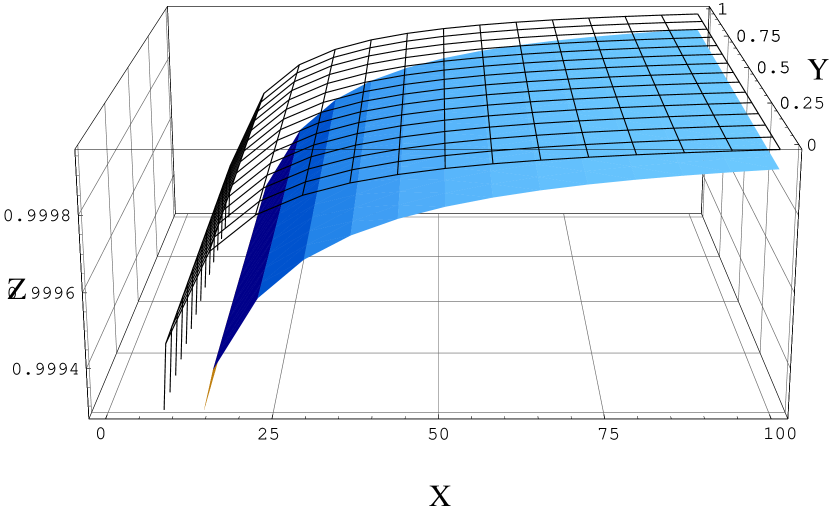
Figure 6.1: ${\cal E}_{\rm ELLPW}$ and ${\cal E}_{\rm KM}$ on Z-axis are plotted against ${\cal R}$ on X-axis and ${\cal S}$ on Y-axis for ${\cal Q}=0.1$. The upper (transparent one) and lower surfaces are for ${\cal E}_{\rm ELLPW}$ and ${\cal E}_{\rm KM}$ respectively.

Now defining

$${\cal E}_{{\rm ELLPW}}:=\frac{E_{{\rm ELLPW}}}{M},\quad{\cal E}_{{\rm ELLPW}}:=\frac{E_{{\rm ELLPW}}}{M},\quad{\cal E}_{{\rm KM}}:=\frac{E_{{\rm K}}}{M}=\frac{E_{{\rm M\o l}}}{M},$$

$${\cal S}:=\frac{a}{M},\quad{\cal Q}:=\frac{e}{M},\quad{\cal R}:=\frac{\rho}{M}$$ (6.17)

the equations $(\ref{EKomar})$, $(\ref{EELLPW})$ and $(\ref{EMol})$ may be expressed as

$${\cal E}_{{\rm ELLPW}}=1-\frac{{\cal Q}^{2}}{4{\cal R}}\left[1+\left(\frac{{\cal S}}{{\cal R}}+\frac{{\cal R}}{{\cal S}}\right)\arctan\left(\frac{{\cal S}}{{\cal R}}\right)\right],$$ (6.18)

and

$${\cal E}_{{\rm KM}}=1-\frac{{\cal Q}^{2}}{2{\cal R}}\left[1+\left(\frac{{\cal S}}{{\cal R}}+\frac{{\cal R}}{{\cal S}}\right)\arctan\left(\frac{{\cal S}}{{\cal R}}\right)\right]\text{\ .}$$ (6.19)

The ring curvature singularity in the KN metric is covered by the event horizon for $\left({\cal Q}^{2}+{\cal S}^{2}\right)\leq 1$ and is naked for $\left({\cal Q}^{2}+{\cal S}^{2}\right)>1$. In Fig. 1 we plot ${\cal E}_{{\rm ELLPW}}$ and ${\cal E}_{{\rm KM}}$ against ${\cal R}$ and ${\cal S}$ for ${\cal Q}=0.1$. As the value of ${\cal R}$ increases the two surfaces shown in the figure come closer.

6.4 Conclusions

The prescriptions of Einstein, Landau and Lifshitz, Papapetrou, and Weinberg used for calculating the energy-momentum distribution in a general relativistic system restrict one to make calculations in quasi-Cartesian coordinates. This shortcoming of singling out a particular coordinate system prompted Møller[46] to construct an expression which enables one to evaluate energy in any coordinate system. According to Møller[46] this expression should give the same values for the total energy and momentum as the Einstein’s energy-momentum complex for a closed system. However, Møller’s energy-momentum complex was subjected to some criticism (see in Møller[47], Kovacs[39], Novotny[50]). Further Komar[38] formulated a new definition of energy in a curved space-time. This prescription, though not restricted to the use of “Cartesian coordinates”, is applicable only to the stationary space-times. The Møller energy-momentum complex is neither restricted to the use of particular coordinates nor to the stationary space-times. Recently, Lessner[41] pointed out that the Møller definition is a powerful concept of energy and momentum in general relativity. However, it is worth noting that for the Reissner-Nordström metric $E_{{\rm ELLPW}}=M-e^{2}/(2\rho)$ (the Penrose definition also gives the same result[74] and this provides the weak field limit) whereas $E_{{\rm KM\o l}}=M-e^{2}/\rho$ does not give the weak field limit. This question must be investigated carefully. In the next chapter we investigate the Cooperstock hypothesis for the non-static space-times with Møller’s energy-momentum complex.

Chapter 7 Energy of the Nonstatic Spherically Symmetric Metrics

7.1 Introduction

In a recent paper, Virbhadra[74] investigated whether or not the energy-momentum complexes of Einstein, Landau and Lifshitz (LL) , Papapetrou, and Weinberg give the same energy distribution for the most general nonstatic spherically symmetric metric and, contrary to previous results of many asymptotically flat spacetimes [1, 12, 13, 21, 63, 64, 65, 66, 67, 68, 70, 72, 77, 78] and asymptotically non-flat spacetimes [56, 70, 79, 80], he found that these definitions disagree. He observed that the energy-momentum complex of Einstein gave a consistent result for the Schwarzschild metric whether one calculates in Kerr-Schild Cartesian coordinates or Schwarzschild Cartesian coordinates. The prescriptions of LL, Papapetrou and Weinberg furnish the same result as in the Einstein prescription if computations are carried out in Kerr-Schild Cartesian coordinates; however, they disagree with the Einstein definition if computations are done in Schwarzschild Cartesian coordinates. Thus, the definitions of LL, Papapetrou and Weinberg do not furnish a consistent result. Based on this and some other investigations (see also in Bergqvist[5], Bernstein and Tod [4], Virbhadra concluded that the Einstein method seems to be the best among all known (including quasi-local mass definitions) for energy distribution in a space-time.

In the previous chapter we highlighted Lessner’s arguments indicating the importance of the Møller energy-momentum expression. So in the present chapter we wish to revisit the Møller energy-momentum prescription by presenting the result of our investigation [83] of the energy distribution in the most general nonstatic spherically symmetric space-time using Møller’s energy-momentum complex. This result is compared with the Virbhadra energy expression obtained by using the energy-momentum complex of Einstein. We also discuss some examples of energy distributions in different prescriptions. In the next section we give the energy expression obtained by Virbhadra[74].

7.2 Virbhadra’s energy result

The most general nonstatic spherically symmetric space-time is described by the line element

$$ds^{2}=\alpha(r,t)\,dt^{2}-\beta(r,t)\,dr^{2}-2\gamma(r,t)\,dt\,dr-\sigma(r,t)\,r^{2}\,(d\theta^{2}+\sin^{2}\theta\,d\phi^{2})\text{.}$$ (7.1)

This has, amongst others, the following well-known space-times as special cases: The Schwarzschild metric, Reissner-Nordström metric, Vaidya metric, Janis-Newman-Winicour metric, Garfinkle-Horowitz-Strominger metric, a general non-static spherically symmetric metric of the Kerr-Schild class (discussed in Virbhadra’s paper[74]). Virbhadra[74] explored the energy distribution in the most general nonstatic spherically symmetric space-time (7.1) using the energy-momentum complex of Einstein (2.16). To compute the energy $E$ ($=P_{0}$) using the $\Theta_{0}{}^{0}$ component of the Einstein energy-momentum complex Virbhadra transformed the line element $(\ref{Genmetric})$ to “Cartesian coordinates” $(t,x,y,z)$ using $x=r\sin\theta\cos\phi,y=r\sin\theta\sin\phi,z=r\cos\theta$ and $t$ remaining the same. Then using (2.20) he obtained the energy distribution which is given below:

$$E_{\rm Einst}=\frac{r\left[\alpha\left(\beta-\sigma-r\sigma_{,r}\right)-\gamma\left(r\sigma_{,t}-\gamma\right)\right]}{2\sqrt{\alpha\beta+\gamma^{2}}}$$ (7.2)

where comma indicates partial differentiation. In the next Section we obtain the energy distribution for the same metric in Møller’s formulation.

7.3 Energy distribution in Møller’s formulation

In this Section we use the energy-momentum complex of Møller to obtain energy distribution in the most general nonstatic spherically symmetric metric given by the equation $(\ref{Genmetric})$. Since the Møller complex is not restricted to the use of “Cartesian coordinates” we perform the computations in $t,r,\theta,\phi$ coordinates, because computations in these coordinates are easier compared to those in $t,x,y,z$ coordinates.

The Møller energy-momentum complex ${\Im}_{i}^{\ k}$ is given by (2.47), with the anti-symmetric superpotential ${\chi}_{i}^{\ kl}$ given by (2.48). To compute the energy distribution

$$E=\frac{1}{8\pi}\int\int{\chi}_{0}^{\ 0\beta}\mu_{\beta}dS,$$ (7.3)

for the line element $(\ref{Genmetric})$ under consideration we calculate

$${\chi}_{0}^{\ 01}=\frac{\left(\alpha_{,r}+\gamma_{,t}\right)\sigma r^{2}\sin\theta}{\left(\alpha\beta+\gamma^{2}\right)^{1/2}}\text{\ ,}$$ (7.4)

which is the only required component of ${\chi}_{i}^{kl}$ for our purpose.

Using the above expression in equation $(\ref{energy})$ we obtain the energy distribution

$$E_{\rm M\o l}=\frac{\left(\alpha_{,r}+\gamma_{,t}\right)\sigma r^{2}}{2\left(\alpha\beta+\gamma^{2}\right)^{1/2}}\text{ \ .}$$ (7.5)

It is evident that the energy distribution for the most general nonstatic spherically symmetric metric the definitions of Einstein and Møller disagree in general (compare $(\ref{EEinst})$ with $(\ref{EMol})$). However, these furnish the same results for some space-times, for instance, the Schwarzschild and Vaidya space-times[66]. In the next Section we will compute energy distribution in a few space-times using $(\ref{EEinst})$ and $(\ref{EMol})$.

7.4
Examples

In this Section we discuss a few examples of space-times in the Einstein as well as the Møller prescriptions. We also test the Cooperstock hypothesis with these examples.

1. The Schwarzschild solution
   This solution is expressed by the line element

   $$ds^{2}=\left(1-\frac{2M}{r}\right)dt^{2}-\left(1-\frac{2M}{r}\right)^{-1}dr^{2}-r^{2}\left(d\theta+\sin^{2}\theta^{2}d\phi^{2}\right)\text{\ .}$$ (7.6)

   Equations $(\ref{EEinst})$ and $(\ref{EMol})$ furnish (see also in [46, 72])

   $$E_{\rm Einst}=E_{\rm M\o l}=M$$ (7.7)

   showing that these two definitions of energy distribution agree for the Schwarzschild space-time and the above results support the Cooperstock hypothesis.

2. The Reissner-Nordström solution
   The Reissner-Nordström solution is given by

   $$ds^{2}=\left(1-\frac{2M}{r}+\frac{e^{2}}{r^{2}}\right)dt^{2}-\left(1-\frac{2M}{r}+\frac{e^{2}}{r^{2}}\right)^{-1}dr^{2}-r^{2}\left(d\theta^{2}+\sin^{2}\theta d\phi^{2}\right)\text{\ ,}$$ (7.8)

   and the antisymmetric electromagnetic field tensor

   $$F_{tr}=\frac{e}{r^{2}}\text{\ ,}$$ (7.9)

   where $M$ and $e$ are respectively the mass and electric charge parameters.

   For this space-time equations $(\ref{EEinst})$ and $(\ref{EMol})$ furnish (see also in [64, 21])

   $$E_{\rm Einst}=M-\frac{e^{2}}{2r}$$ (7.10)

   and

   $$E_{\rm M\o l}=M-\frac{e^{2}}{r}\text{\ .}$$ (7.11)

   Both of these results obviously support the Cooperstock hypothesis.

3. The Janis-Newman-Winicour solution

   This solution has been usually incorrectly referred to in the literature as the Wyman solution. Virbhadra[72] proved that the Wyman solution is the same as the Janis-Newman-Winicour solution. As Janis, Newman and Winicour obtained this solution much before Wyman, Virbhadra[74] rightly referred to this as the Janis-Newman-Winicour solution. This solution is given by

   $$ds^{2}=\left(1-\frac{B}{r}\right)^{\mu}dt^{2}-\left(1-\frac{B}{r}\right)^{-\mu}dr^{2}-\left(1-\frac{B}{r}\right)^{1-\mu}r^{2}\left(d\theta^{2}+\sin^{2}\theta\ d\phi^{2}\right)$$ (7.12)

   and the scalar field

   $$\Phi=\frac{q}{B\sqrt{4\pi}}\ln\left(1-\frac{B}{r}\right),$$ (7.13)

   where

   $$\mu = \frac{2M}{B},$$

   $$B = 2\sqrt{M^{2}+q^{2}}.$$ (7.14)

   $M$ and $q$ are the mass and scalar charge parameters respectively. For $q=0$ this solution furnishes the Schwarzschild solution.

   Virbhadra[74] computed the energy expression for this metric using Eq. $(\ref{EEinst})$. We do the same here using equation $(\ref{EMol})$. Thus we find that

   $$E_{\rm Einst}=E_{\rm M\o l}=M\text{,}$$ (7.15)

   which shows that these two definitions of energy distribution agree for the Janis-Newman-Winicour space-time.

4. Garfinkle-Horowitz-Strominger solution

   The Garfinkle-Horowitz-Strominger static spherically symmetric asymptotically flat solution (see in [27]) is described by the line element (3.3). In order to compute the energy distribution in Garfinkle-Horowitz-Strominger space-time using the energy-momentum complex of Einstein, Chamorro and Virbhadra[12] transformed (3.3) to quasi-Cartesian coordinates (3.8) . Then, by making use of (2.16) they found the following expression in Einstein prescription:

   $$E_{\rm Einst}=M-\frac{e^{2}}{2r}\left(1-\lambda^{2}\right)\text{\ .}$$ (7.16)

   We compute the energy distribution for the Garfinkle-Horowitz-Strominger space-time using equation $(\ref{EMol})$ and obtain

   $$E_{\rm M\o l}=M-\frac{e^{2}}{r}\left(1-\lambda^{2}\right)\text{\ .}$$ (7.17)

   Thus, these two definitions give different results (there is a difference of a factor $2$ in the second term) but they obviously support the Cooperstock hypothesis.

   Now defining

   $${\cal E}_{\rm Einst}:=\frac{E_{\rm Einst}}{M},\quad{\cal E}_{\rm M\o l}:=\frac{E_{\rm M\o l}}{M},\quad{\cal Q}:=\frac{e}{M},\quad{\cal R}:=\frac{r}{M}$$ (7.18)

   the equations $(\ref{GHSEE})$ and $(\ref{GHSME})$ may be expressed as

   $${\cal E}_{\rm Einst}=1-\frac{{\cal Q}^{2}}{2{\cal R}}\left(1-\lambda^{2}\right)$$ (7.19)

   and

   $${\cal E}_{\rm M\o l}=1-\frac{{\cal Q}^{2}}{{\cal R}}\left(1-\lambda^{2}\right)$$ (7.20)

   For $\lambda^{2}=1,{\cal E}_{\rm Einst}={\cal E}_{\rm M\o l}=M$; however, they differ for any other values of $\lambda^{2}$. For any values of $\lambda^{2}<1$, ${\cal E}_{\rm Einst}$ as well as ${\cal E}_{\rm M\o l}$ decrease with an increase in ${\cal Q}^{2}$ and increase with increase in ${\cal R}$. ${\cal E}_{\rm Einst}>{\cal E}_{\rm M\o l}$ and they asymptotically ($\cal R\rightarrow\infty$) reach the value $1$. The situation is just opposite for any values of $\lambda^{2}>1$ : ${\cal E}_{\rm Einst}$ as well as ${\cal E}_{\rm M\o l}$ increase with an increase in ${\cal Q}^{2}$ and decrease with increase in $R$. ${\cal E}_{\rm Einst}<{\cal E}_{\rm M\o l}$ and they asymptotically ($\cal R\rightarrow\infty$) reach the value $1$.

   We plot the energy distributions ${\cal E}_{\rm Einst}$ and ${\cal E}_{\rm M\o l}$ for $\lambda=0$ (Reissner-Nordström space-time) in the figure 1 and for $\lambda^{2}=1.2$ in figure 2.

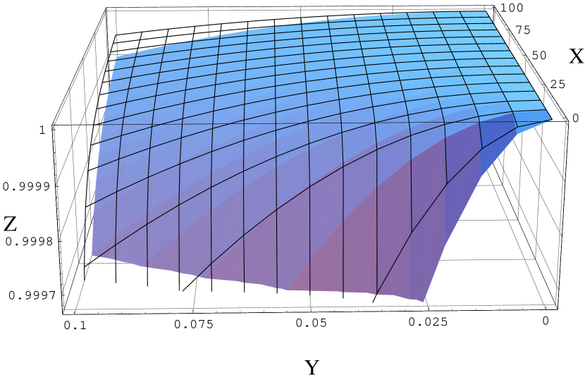
Figure 7.1: ${\cal E}_{\rm Einst}$ and ${\cal E}_{\rm M\o l}$ on Z-axis are plotted against ${\cal R}$ on X-axis and ${\cal Q}$ on Y-axis for ${\lambda}=0$ (Reissner-Nordström metric). The upper (grid-like) and lower surfaces are for ${\cal E}_{\rm Einst}$ and ${\cal E}_{\rm M\o l}$ respectively.

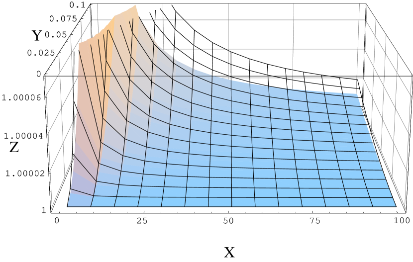
Figure 7.2: ${\cal E}_{\rm Einst}$ and ${\cal E}_{\rm M\o l}$ on Z-axis are plotted against ${\cal R}$ on X-axis and ${\cal Q}$ on Y-axis for ${\lambda^{2}}=1.2$. The upper (grid-like) and lower surfaces are for ${\cal E}_{\rm M\o l}$ and ${\cal E}_{\rm Einst}$ respectively.

7.5
Conclusion

Based on some analysis of the results known with many prescriptions for energy distribution (including some well-known quasi-local mass definitions) in a given space-time Virbhadra[74] remarked that the formulation by Einstein is still the best one. Lessner[41] argued that the Møller energy-momentum expression is a powerful concept of energy and momentum in general relativity, which motivated us to study this further. We obtained the energy distribution for the most general nonstatic spherically symmetric metric using Møller’s definition. The result we found differs in general from that obtained using the Einstein energy-momentum complex. However, these agree for the Schwarzschild, Vaidya and Janis-Newman-Winicour space-times. They disagree for the Reissner-Nordström space-time. For the Reissner-Nordström space-time $E_{\rm Einst}=M-e^{2}/(2r)$ (the seminal Penrose quasi-local mass definition also yields the same result agreeing with linear theory[59]) whereas $E_{\rm M\o l}=M-e^{2}/r$. This question must be considered important. Møller’s energy- momentum complex is not constrained to the use of any particular coordinates (unlike the case of the Einstein complex); however, as we have shown above, it does not furnish expected result for the Reissner-Nordström space-time. We agree with Virbhadra’s conclusion that the Einstein energy-momentum complex is still the best tool for obtaining energy distribution in a given space-time.

Chapter 8 Summary and Conclusion

An important feature of conserved quantities such as the energy, momentum and angular momentum is that they play a very fundamental role in any physical theory as they provide a first integral of equations of motion (Nahmad-Achar and Schutz[48]). These help to solve, what would otherwise be, intractable problems, for instance, collisions, stability properties of physical systems etc. Conservation laws of energy-momentum, together with the equivalence principle, played a significant role in guiding Einstein’s search for generally covariant field equations. Evidently, it is desirable to incorporate conserved quantities in general relativity. Energy-momentum is an important conserved quantity whose definition has been a focus of many investigations. Unfortunately, there is still no generally agreed definition of energy and momentum in general relativity.

Einstein’s formulation of energy-momentum conservation laws in the form of a divergence to include contribution from gravitational field involved the introduction of a pseudotensor quantity $t_{j}{}^{i}$. Owing to the fact that $t_{j}{}^{i}$ is not a true tensor (although covariant under linear transformations), Levi-Civita, Schrödinger, and Bauer expressed some doubts at the validity of Einstein’s energy-momentum conservation laws. Although, Einstein defended the use of a pseudotensor quantity to represent gravitational field and showed that his energy-momentum pseudocomplex provides satisfactory expressions for the total energy and momentum of closed systems, the problems associated with Einstein’s energy-momentum complex, used for calculating the energy and momentum distribution in a general relativistic system, was followed by many definitions, some of which are coordinate dependent and others are not. The physical meaning of these was questioned, and the large number of the definitions of energy-momentum complexes only fuelled scepticism that different energy-momentum complexes could give unacceptable different energy distribution for a given space-time. The problems associated with energy-momentum complexes resulted in some researchers even doubting the concept of energy-momentum localization.

Misner et al [45] argued that to look for a local energy-momentum is looking for the right answer to the wrong question. They further argued that energy is only localizable for spherical systems. Cooperstock and Sarracino [22] countered this point of view, arguing that if energy is localizable in spherical systems then it is localizable in any space-times. Bondi[6] noted that a nonlocalizable form of energy is not admissible in general relativity. The viewpoints of Misner et al discouraged further study of energy localization and on the other hand an alternative concept of energy, the so-called quasi-local energy, was developed. To date, a large number of definitions of quasi-local mass have been proposed. The uses of quasi-local masses to obtain energy in a curved space-time are not limited to a particular coordinates system whereas many energy-momentum complexes are restricted to the use of “Cartesian coordinates.” Penrose[53] emphasized that quasi-local masses are conceptually very important. Nevertheless, the present quasi-local mass definitions still have inadequacies. For instance, Bergqvist[5] considered quasi-local mass definitions of Komar, Hawking, Penrose, Ludvigsen-Vickers, Bergqvist-Ludvigsen, Kulkarni-Chellathurai-Dadhich, and Dougan-Mason and concluded that no two of these definitions give agreed results for the Reissner-Nordstrøm and Kerr space-times. The shortcomings of the seminal quasi-local mass definition of Penrose in handling the Kerr metric are discussed in Bernstein and Tod[4], and in Virbhadra[74]. On the contrary, the remarkable work of Virbhadra, and some others, and recent results of Chang, Nester and Chen have revived the interest in various energy-momentum complexes.

Virbhadra, and co-workers considered many space-times and have shown that several energy-momentum complexes give the same and acceptable results for a given space-time. Aguirregabiria et al. [1] proved that several energy-momentum complexes “coincide” for any Kerr-Schild class metric. Virbhadra [74] showed that for a general non-static spherically symmetric metric of the Kerr-Schild class, the energy-momentum complexes of Einstein, Landau and Lifshitz, Weinberg and Papapetrou furnish the same result as Tod obtained using the Penrose quasi-local mass definition. These are fascinating results. Recently, Chang, Nester and Chen [14] demonstrated that by associating each of the energy-momentum complexes of Einstein, Landau and Lifshitz, Møller, Papapetrou, and Weinberg with a legitimate Hamiltonian boundary term, then each of these complexes may be said to be quasi-local. Quasi-local energy-momentum are obtainable from a Hamiltonian. Hence energy-momentum complexes are useful expressions for computing energy distributions.

Virbhadra and Parikh [67] calculated, using the energy-momentum complex of Einstein, the energy distribution for a spherically symmetrically charged black hole in low-energy string theory and found that the energy is confined to the interior of the holes. Using Einstein’s energy-momentum complex, Chamorro and Virbhadra [12] studied the energy distribution associated with static spherically symmetric charged dilaton black holes for an arbitrary value of the coupling parameter which controls the strength of the dilaton to the Maxwell field, and got an acceptable result. We [77, 78], (for a discussion see chapter 3) computed energy distributions in these space-times using the Tolman form of the Einstein’s complex and confirmed both of the above computations. In the case of static spherically symmetric charged dilaton black holes the energy distribution depends on the value of the coupling parameter while the total energy does not depend on this parameter.

Earlier investigations [12, 13, 21, 63, 64, 65, 66, 67, 68, 72] with many asymptotically flat space-times indicated that several energy-momentum complexes give the same and acceptable result for a given space-time. Rosen and Virbhadra [56, 71] showed, using the Einstein-Rosen space-time, that even for an asymptotically nonflat space-time many energy-momentum complexes could give the same and persuading results. We[79] computed the energy distribution in the Ernst space-time, using the Einstein energy-momentum complex and got encouraging results. This prompted us to investigate energy distribution in Melvin’s magnetic universe (which is a special case of Ernst space-time) using several different energy-momentum complexes. We[81] found that the energy-momentum complexes of Einstein, Landau and Lifshitz, and Papapetrou give the same and acceptable energy distribution in Melvin’s magnetic universe(for a discussion see chapter 4) . These results uphold the importance of energy-momentum complexes.

The work of Rosen[55] and Cooperstock [18] on the energy of the universe was followed by the investigations of Johri et al [37], and Banerjee and Sen [3]. These researchers studied the energy content of the universe using different models. Using the Einstein energy-momentum complex, Rosen [55] studied the total energy of a closed homogeneous isotropic universe described by the Friedmann-Robertson-Walker (FRW) metric and found that to be zero. Cooperstock [18] concluded, after making use of calculations involving killing vectors, that for a conformal Friedmann-Robertson-Walker metric the total energy density is equal to zero. Johri et al. [37] showed, using the Landau and Lifshitz definition, that the total energy of an FRW spatially closed universe is zero at all times irrespective of equations of state of the cosmic fluid. They also showed that the total energy enclosed within any finite volume of the spatially flat FRW universe is zero at all times. Using the energy-momentum complex of Einstein, Banerjee and Sen [3] showed that the energy and momentum density components vanish in the Bianchi type I space-times. We[80] extended the investigations of Banerjee and Sen with the energy-momentum complexes of Landau and Lifshitz, Papapetrou, and Weinberg to check whether these complexes could give different results for the Bianchi type I space-times. We got the same results as obtained by Banerjee and Sen [3] (for a discussion see chapter 5).

The Kerr-Newman (KN) solution is the most general black hole solution to the Einstein-Maxwell equations. Cohen and de Felice [16] investigated energy distribution in this space-time using Komar’s prescription. This was followed by the investigations of Virbhadra [63, 64] and Cooperstock and Richardson [21] who showed (up to the third order and seventh order, respectively, of rotation parameter) that the energy-momentum complexes of Einstein and Landau-Lifshitz give the same and reasonable energy distribution in KN space-time. Aguirregabiria et al. [1] performed exact computations for the KN energy distribution,in the prescriptions of Einstein, Landau-Lifshitz, Papapetrou, and Weinberg (ELLPW) in Kerr-Schild Cartesian coordinates. They showed that the ELLPW complexes again gave the same energy distribution, but the second term of their result differs by a factor of two from that obtained by Cohen and de Felice. Seeing the results that the ELLPW all give the same energy distribution, and Lessner’s[41] conclusion that Møller’s energy-momentum expression is a powerful representation of energy and momentum we found it tempting to obtain energy using this prescription. We first note that Florides [26] showed that for all static or quasi-static space-times, the Møller’s energy formula is equivalent to the Tolman’s energy formula (Eq. 2.27). We[82] evaluated the energy distribution for the KN space-time in Møller’s prescription. We found that the energy distribution in KN space-time computed using Møller energy-momentum complex agrees with Komar mass obtained by Cohen and de Felice[16]. We also found that our results support the Cooperstock hypothesis (for a discussion see chapter 6).

As already discussed, it has been shown with examples of many space-times that several energy-momentum complexes give the same and acceptable energy distribution for a given space-time. Recently Virbhadra[74] investigated whether or not several energy-momentum complexes give the same result for the most general nonstatic spherically symmetric metric, and contrary to previous results, he found that the prescriptions of Einstein, Landau and Lifshitz, Papapetrou, and Weinberg all give different results. Based on some analysis of the results known with many prescriptions for energy distribution (including some well-known quasi-local mass definitions) in a given space-time Virbhadra[74] concluded that the formulation by Einstein is still the best one. In order to test the validity of Virbhadra’s conclusion and to further investigate the Cooperstock hypothesis we[83] used the Møller’s energy-momentum complex to study the energy distribution in the most general nonstatic spherically symmetric space-time considered by Virbhadra [74]. The Møller energy distribution differs in general from that obtained using the Einstein energy-momentum complex. Both prescriptions agree for the Schwarzschild, Vaidya and Janis-Newman-Winicour space-times, but disagree for the Reissner-Nordström space-time. For the Reissner-Nordström space-time both the Einstein prescription and the Penrose quasi-local mass definition yields the same result which agrees with linear theory. This confirms Virbhadra’s conclusion that Einstein’s prescription is still the best tool for finding energy distribution in a given space-time.

The main weaknesses of energy-momentum complexes is that most of these restrict one to make calculations in “Cartesian coordinates”, and the large number of these energy-momentum complexes makes it difficult to decide as to which one to use to compute energy-momentum distribution - given the suspicion these would give different energy-momentum distributions for a given space-time. The alternative concept of quasi-local mass is more attractive because these are not restricted to the use of any special coordinate system. There is a large number of definitions of quasi-local masses. It has been shown[5] that for a given space-time many quasi-local mass definitions do not give agreed results. On the other hand previous results[1] and our results [79, 80, 81] show that for many space-times several energy-momentum complexes give the same and acceptable energy-momentum for a given space-time. The important paper of Chang,et al[14] dispels doubts expressed about the physical meaning of these energy-momentum complexes. Our results [82, 83] support Virbhadra’s conclusion that Einstein’s energy-momentum complex is still the best available method for computing energy-momentum in a given space-time. These results also support the Cooperstock hypothesis that the energy and momentum in a curved space-time are confined to the regions of non-vanishing energy-momentum tensor $T_{i}^{\ k}$ of the matter and all non-gravitational fields.

Bibliography

- [1] Aguirregabiria, J. M., Chamorro, A. and Virbhadra, K. S., Gen. Relativ. Gravit. 28, 1393 (1996).
- [2] Bak, D., Cangemi, D. and Jackiw, R., Phys. Rev. D42, 5173 (1994).
- [3] Banerjee, N. and Sen, S., Pramana-Journal of Physics, 49, 609 (1997).
- [4] Bernstein, D. H. and Tod, K. P., Phys. Rev. D49, 2808 (1994).
- [5] Bergqvist, G., Class. Quantum Gravit. 9, 1753 (1992).
- [6] Bondi, H., Proc. R. Soc. London A427, 249 (1990).
- [7] Bringley, T., Mod. Phys. Lett. A17, 157 (2002).
- [8] Brown, J. D. and York, Jr. J. W., Phys. Rev.D47, 1407 (1993).
- [9] Carmeli, M., Classical Fields: General Relativity and Gauge Theory, (John Wiley & Sons, 1982).
- [10] Carter, B., Phys. Rev. 174, 1559 (1968).
- [11] Cattani, C. and De Maria, M., in The attraction of Gravitation: New Studies in the History of General Relativity, Einstein Studies Volume 5, Edited by Earman, J., Janssen, M. and Norton, J. D. (The Center for Einstein Studies, 1993), pp. 63 - 87.
- [12] Chamorro, A. and Virbhadra, K. S., Int. J. Mod. Phys.D5, 251 (1996).
- [13] Chamorro, A. and Virbhadra, K. S., Pramana-J. Phys.45, 181 (1995).
- [14] Chang, C. C., Nester, J. M. and Chen, C., Phys. Rev. Lett. 83, 1897 (1999).
- [15] Chandrasekhar, S. and Ferrari, V., Proc. R. Soc. London A435, 645 (1991).
- [16] Cohen, J. M. and de Felice, F., J. Math. Phys.,25, 992 (1984).
- [17] Cooperstock, F. I., in Topics on Quantum Gravity and Beyond, Essays in honour of L. Witten on his retirement, edited by F. Mansouri and J. J. Scanio (World Scientific, Singapore, 1993).
- [18] Cooperstock, F. I., General Relativity and Gravitation, 26, 323 (1994).
- [19] Cooperstock, F. I., Mod. Phys Lett. A14, 1531 (1999).
- [20] Cooperstock, F. I., Annals of Phys. 282, 115 (2000).
- [21] Cooperstock, F. I. and Richardson, S. A., in Proc. 4th Canadian Conf. on General Relativity and Relativistic Astrophysics (World Scientific, Singapore, 1991).
- [22] Cooperstock, F. I. and Sarracino, R. S. J. Phys. A: Math. Gen. 11, 877 (1978).
- [23] Einstein, A., The Foundation of the General Theory of Relativity a translation of the 1916 paper in The Principle of Relativity : a collection of original papers … by Lorentz et. al. (Dover Publications, Inc.)
- [24] Ernst, F. J., J. Math. Phys. 15, 1409 (1974); 17, 54 (1976).
- [25] Feynmann, R. P., Leighton, R. B. and Sands, M. (1979). The Feynman Lectures on Physics vol 2, Reading, Mass: Addison-Wesley, ch. 27.
- [26] Florides, P. S., General Relativity and Gravitation, 26, 1145 (1994).
- [27] Garfinkle, D., Horowitz, G. T. and Strominger, A. Phys. Rev. D43, 3140 (1991); Erratum: Phys. Rev. D45, 3888 (1992).
- [28] Goldberg, J. N. in General Relativity and Gravitation: One Hundred Years After the Birth of Albert Einstein, Volume 1 Edited by A. Held (Plenum Press, NY, 1980).
- [29] Gupta, S. N., Phys. Rev. 96, 1683 (1954).
- [30] Havas, P., in Developments in General Relativily, Astrophysics and Quantum Theory, A Jubilee Volume in Honour of Nathan Rosen, Annals of the Israel Physical Society Volume 9, Edited by F. I. Cooperstock, L. P. Horwitz and J. Rosen (I.O.P. Publishing Ltd, Bristol, and the Israel Physical Society in association with the American Institute of Physics, 1990).
- [31] Hayward, S. A., Phys. Rev. D49, 831 (1994).
- [32] Holzhey, C. F. E. and Wilczek, F., Nucl. Phys. B380, 447 (1992).
- [33] Horne, J. H. and Horowitz, G. T., Phys. Rev. D46, 1340 (1992).
- [34] Shapere, A., Trivedi, S. and Wilczek, F. , Mod. Phys. Lett. A6, 2677 (1991); Shiraishi, K. Phys. Lett. A166, 298 (1992); Harvey, J. A. and Strominger, A., Quantum aspects of black holes, hep-th/9209055; Dowker, F. , Gauntlett, J. P., Kastor, D. A. and Traschen, J. Phys. Rev. D49, 2909 (1994).
- [35] Israel, W., in Three hundred years of gravitation Edited by Hawking, S. W. and Israel, W. (Cambridge University Press, Cambridge, 260 (1987).
- [36] Janis, A. I., Newman, E. T. and Winicour, J., Phys. Rev. Lett. 20, 878 (1968).
- [37] Johri, V. B., Kalligas, D., Singh, G. P. and Everitt, C. W. F., General Relativity and Gravitation, 27, 313 (1995).
- [38] Komar A.,, Phy. Rev. 113, 934 (1959).
- [39] Kovacs, D., Gen. Relativ. Gravit.. 17, 927 (1985).
- [40] Landau, L. D. and Lifshitz, E.M., The Classical Theory of Fields, Pergamon Press, p. 280 (1987).
- [41] Lessner, G., Gen. Relativ. Gravit. 28, 527 (1996).
- [42] Melvin, M. A., Phys. Lett. 8, 65 (1964).
- [43] Melvin, M. A., Phys. Rev. 139 , B225 (1965).
- [44] Misra, M. and Radhakrishna, L. , Proc. Natl. Inst. Sci. India 28 A 632 (1962).
- [45] Misner, C. W., Thorne, K. S. and Wheeler, J. A., Gravitation, W. H. Freeman and Co., NY, p.603 (1973).
- [46] Møller, C., Annals of Physics (NY) 4, 347 (1958).
- [47] Møller, C., Annals of Physics (NY) 12, 118 (1961).
- [48] Nahmad-Achar, E. and Schutz, B. F., Gen. Relativ. Gravit.. 19, 655 (1987).
- [49] Norton, J.D. in Einstein and the History of General Relativity, Einstein Studies Volume 1, Edited by Howard, D. and Stachel, J. (The Center for Einstein Studies, 1989), pp. 101 - 159.
- [50] Novotny, J., Gen. Relativ. Gravit.. 19, 1043 (1987).
- [51] Papapetrou, A. (1948). Proceedings of the Royal Irish Academy A, 52, 11.
- [52] Pauli, W. Theory of Relativity, Translated from the German by G. Field. (The Pergamon Press, Ltd, 1958).
- [53] Penrose, R., Proc. Roy. Soc. London A381, 53 (1982).
- [54] Rosen, N., Phys. Rev. 110, 291 (1958).
- [55] Rosen, N., General Relativity and Gravitation, 26, 319 (1994).
- [56] Rosen, N. and Virbhadra, K. S., Gen. Relativ. Gravit. 25, 429 (1993).
- [57] Schroder U. E., Special Relativity, World Scientific Lecture Notes in Physics Volume 33, (World Scientific, 1990)
- [58] Thorne, K. S., Phys. Rev. 139 , B244 (1965).
- [59] Tod, K. P., Proceedings of Royal Society of London A388, 467 (1983).
- [60] Tolman, R. C., Phys. Rev. 35, 875 (1930).
- [61] Tolman, R. C., Relativity, Thermodynamics and Cosmology (Oxford Univ. Press, London, 1934) p. 227.
- [62] Tryon, E. P., Nature, 246, 396 (1973).
- [63] Virbhadra, K. S., Phys. Rev. D42, 1066 (1990).
- [64] Virbhadra, K. S., Phys. Rev. D42, 2919 (1990). Virbhadra, K. S., Pramana - J. Phys. 45, 215 (1995).
- [65] Virbhadra, K. S., Mathematics Today 9, 39 (1991).
- [66] Virbhadra, K. S., Pramana-J. Phys. 38, 31 (1992).
- [67] Virbhadra, K. S., and Parikh, J. C. Phys. Lett. B317, 312 (1993).
- [68] Virbhadra, K. S., and Parikh, J. C. Phys. Lett. B331, 302 (1994).
- [69] Virbhadra, K. S. and Prasanna, A. R., Pramana - J. Phys. 33 , 449 (1989).
- [70] Virbhadra, K. S., Pramana - J. Phys. 44, 317 (1995).
- [71] Virbhadra, K. S., Pramana - J. Phys. 45, 215 (1995).
- [72] Virbhadra, K. S., Int. J. Mod. Phys. A12, 4831 (1997).
- [73] Virbhadra, K. S., Jhingan, S. and Joshi, P. S., Int. J. Mod. Phys. D6, 357 (1997).
- [74] Virbhadra, K. S., Phys. Rev. D60, 104041 (1999).
- [75] Weinberg, S., (1972). Gravitation and Cosmology: Principles and Applications of General Theory of Relativity, (John Wiley and Sons, Inc., New York, 1972) p. 165.
- [76] Wheeler, J. A., in Relativity, Groups and Topology, edited by B. and C. DeWitt (Gordon and Breach Publishers, Inc.,N.Y., 1964).
- [77] Xulu, S. S., Int. J. Theor. Phys. 37, 1773 (1998).
- [78] Xulu, S. S., Int. J. Mod. Phys. D7, 773 (1998).
- [79] Xulu, S. S., Int. J. Mod. Phys. A15, 2979 (2000).
- [80] Xulu, S. S., Int. J. Theor. Phys. 39, 1153 (2000).
- [81] Xulu, S. S., Int. J. Mod. Phys. A15, 4849 (2000).
- [82] Xulu, S. S., Mod. Phys. Lett. A15, 1511 (2000).
- [83] Xulu, S. S., Astrophys. and Space Sc. 283, 23 (2003).