Brane Structure from a Scalar Field in Warped Spacetime

Abstract:

We deal with scalar field coupled to gravity in five dimensions in warped geometry. We investigate models described by potentials that drive the system to support thick brane solutions that engender internal structure. We find analytical expressions for the brane solutions, and we show that they are all linearly stable.

Keywords: exd, gra

Branes in higher dimensional theories provide an interesting new procedure for resolving problems involving cosmological constant and hierarchy [1, 2]. The brane scenario that we are interested in the present letter is driven by a single real scalar field. It engenders the interesting feature of localizing massless graviton in the brane, efficiently reproducing four dimensional gravity in the brane. The study of scalar fields coupled to gravity in warped geometries has gained renewed attention recently [3, 4, 5, 6, 7, 8]. In particular, in Ref. [9] one investigates the splitting of thick branes due to a first-order phase transition in a warped geometry. The work of Ref. [9] considers a complex scalar field coupled to gravity, and it shows that when the temperature approaches its critical value, an interface that interpolates two bulk phases breaks into two separated interfaces, giving rise to a new phase which appears in between these two interfaces, leading to an effect which is known in condensed matter as complete wetting — see also Ref. [10] for other details in the subject.

In the present work we show that similar results also appear at zero temperature, in a simpler model, which depends on a single real scalar field, coupled to gravity in five dimensions in a warped geometry. The results seem to be of compelling interest to high energy physics, and are depicted in the figures below. The potential that controls the scalar field depends on odd integers in a very specific manner [11], allowing the appearance of thick branes that host internal structure, in the form of a layer of a new phase squeezed in between two separate interfaces. The potential that we investigate here was first studied in Ref. [11], and there it was shown that although it depends on a single real scalar field, it supports 2-kink solutions of the BPS type, which are stable solutions that solve first order differential equations and engender the feature of being composed of two standard kinks. These topological defects are richer than the standard topological kinks, and they may be seen as defects that host internal structures. This feature establishes the main motivation of this work, in which we explore the possibility to offer a brane scenario where the brane entraps internal structure. The idea is similar to the investigations done in [12, 13] in flat spacetime, in models described by two real scalar fields, and in [14] in curved spacetimes, in brane scenarios involving two higher dimensions. In the present work, however, we shall deal with very specific models, described by a single real scalar field, which couples with gravity in warped spacetime in one higher dimension.

To show how the above potential behaves in the brane scenario, we follow Refs. [6, 8] and we consider the action

$$S=\int d^{4}x\,dy\sqrt{|g|}\Bigl{[}-\frac{1}{4}R+\frac{1}{2}\partial_{a}\phi\partial^{a}\phi-V(\phi)\Bigr{]}$$ (1)

where $g=\det(g_{ab})$ and the metric is

$$ds^{2}=g_{ab}dx^{a}dx^{b}=e^{2A}\eta_{\mu\nu}dx^{\mu}dx^{\nu}-dy^{2}$$ (2)

where $a,b=0,1,2,3,4,$ $\mu,\nu=0,1,2,3,$ $\;\eta_{\mu\nu}=(1,-1,-1,-1)$ and $e^{2A}$ is the warp factor. We suppose that the scalar field and the warp factor only depend on the extra coordinate $y$. In this case the equations of motion are

$$\phi^{\prime\prime}+4A^{\prime}\phi^{\prime} = \frac{dV}{d\phi}$$ (3)

$$A^{\prime\prime} = -\frac{2}{3}\,\phi^{\prime 2}$$ (4)

$$A^{\prime 2} = \frac{1}{6}\phi^{\prime 2}-\frac{1}{3}V(\phi)$$ (5)

where prime stands for derivative with respect to $y$. Our model is given by

$$V_{p}(\phi)=\frac{1}{8}\left(\frac{dW_{p}}{d\phi}\right)^{2}-\frac{1}{3}W^{2}_{p}$$ (6)

where [11]:

$$W_{p}(\phi)=\frac{2p}{2p-1}\,\phi^{\frac{2p-1}{p}}-\frac{2p}{2p+1}\,\phi^{\frac{2p+1}{p}}$$ (7)

The parameter $p$ is odd integer and controls the way the scalar field self-interacts. For clarity, in Fig. [1] we depict the potential $V_{p}(\phi)$ for $p=1,3,5.$

The function $W_{p}(\phi)$ was first introduced in Ref. [11] in flat spacetime. It was inspired in the work on deformed defects [15], and it appears with the help of the deformation prescription there proposed. To see how this is done, we suppose that the spacetime is flat. In this case the potential is given by ${\widetilde{V}}(\phi)=(1/2)(d{\widetilde{W}}/d\phi)^{2}$. We consider the function ${\widetilde{W}}(\phi)=\phi-\phi^{3}/3,$ which identifies the standard $\phi^{4}$ model. We now follow [15] and introduce the function $f(\phi)=\phi^{1/p}$, which is well-defined for every $\phi,$ for $p$ odd integer. This function can be used to change ${\widetilde{W}}(\phi)=\phi-\phi^{3}/3$ to a new model, defined by ${\widetilde{W}}_{p}(\phi)$. The deformation prescription leads to the general result $(df/d\phi)(d{\widetilde{W}}_{p}/d\phi)=(d{\widetilde{W}}/d\phi)[\phi\to f(\phi)],$ where in the right hand side one needs to change $\phi$ by $f(\phi),$ after taking the derivative of ${\widetilde{W}}(\phi).$ For the case under consideration we get ${\widetilde{W}}_{p}(\phi)=(p/2)W_{p}(\phi),$ that is, $(p/2)$ times the expression in Eq. (7), which is used to define the potential $V_{p}(\phi).$

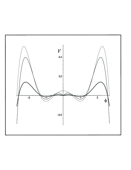
Figure 1: Plots of the potential $V_{p}(\phi)$ for $p=1,3,\;{\rm and}\;5.$ Here and in the other figures the thickness of the lines increases with increasing $p.$

We return to curved spacetime, and we recall that potentials defined as in Eq. (6), through the introduction of the function $W=W(\phi)$, appear very naturally in supergravity, and there $W$ is named superpotential — see Refs.[16, 17, 18] for more details on this subject.

The use of $W_{p}(\phi)$ to define the potential provides an important approach, which leads to first-order equations that solve the equations of motion — see for instance Refs. [19, 20, 6]. The first-order equations are given by

$$\phi^{\prime}=\frac{1}{2}\,\frac{dW_{p}}{d\phi}$$ (8)

and

$$A^{\prime}=-\frac{1}{3}\,W_{p}$$ (9)

The first-order equation for $\phi$ reproduces the first-order equation for the scalar field in flat spacetime [11], apart from the numerical factor of $1/2$. We solve this equation to get [11]

$$\phi_{p}(y)=\tanh^{p}\left(\frac{y}{p}\right)$$ (10)

We see that for $p=1$ we get the standard solution. However, for $p=3,5,...$ we get 2-kink solutions, which we show in Fig. [2] — see Ref. [11] for more details on such defect structures.

Figure 2: Plots of the solutions $\phi_{p}(y)$ for $p=1,3,\;{\rm and}\;5.$

The first-order equation (9) for the warp factor is new for $W_{p}$ given by Eq. (7), and we have been able to solve it for $A_{p}(y)$ analytically. We get

$$A_{p}(y)\!\! = \!\!-\frac{1}{3}\frac{p}{2p+1}\tanh^{2p}\left(\frac{y}{p}\right)-\frac{2}{3}\left(\frac{p^{2}}{2p-1}-\frac{p^{2}}{2p+1}\right)$$ (11)

$$\biggl{\{}\ln\biggl{[}\cosh\left(\frac{y}{p}\right)\biggr{]}-\sum_{n=1}^{p-1}\frac{1}{2n}\tanh^{2n}\left(\frac{y}{p}\right)\biggr{\}}$$

We plot the warp factor $e^{2A_{p}(y)}$ corresponding to these solutions for $p=1,3,5$ in Fig. [3].

The scalar matter field and the warp factor contribute to the brane scenario according to the solutions (10) and (11). We use these results to obtain the matter energy density $T_{00}^{\,p}(y)$ as a function of the extra dimension. The analytic expression for $T_{00}^{\,p}$ is rather awkward, thus we decided to plot it in Fig. [4] to show the matter behavior when $\phi(y)$ and $A(y)$ solve the first order equations (8) and (9), respectively.

Figure 3: Plots of the warp factor $e^{2A_{p}(y)}$ for $p=1,3,\;{\rm and}\;5.$

The plots depicted in Fig. [4] show that the matter field gives rise to thick branes composed of a single $(p=1)$ or two $(p=3,5,...)$ interfaces. In the last case, for $p=3,5,...,$ one sees the appearance of a new phase in between the two interfaces where the energy density of the matter field gets more concentrated. The scenario for $p=3,5,...,$ is that of a brane that supports internal structure [12, 13, 14]. We use Figs. [3] and [4] to see that the warp factor is essencially constant (for $p=3,5,...)$ in the very inside of the brane, in the region where the energy density vanishes. This unveils the presence of a new phase inside the brane, protected by the two interfaces that appear centered at the points which maximize the energy density. For $p=1$ the scenario is quite different, and the brane does not support the internal structure that we clearly see for $p=3,5,...$

Figure 4: Plots of the matter energy density $T^{\,1}_{00}(y)/10,$ $T^{\,3}_{00}(y),$ and $T^{\,5}_{00}(y)$ for $p=1,3,\;{\rm and}\;5.$ We have plotted $1/10$ of $T^{\,1}_{00}$ to ease comparison.

The scalar matter model (7) that we have used leads to the solutions (10) and (11), which are depicted in Figs. [2] and [3], respectively. We go further into the subject and we examine stability of the above braneworld scenario. The key issue here is stability of the geometry induced by the above solutions. We do this perturbing the metric, using

$$ds^{2}=e^{2A(y)}(\eta_{\mu\nu}+h_{\mu\nu})dx^{\mu}dx^{\nu}-dy^{2}$$ (12)

and supposing that $h_{\mu\nu}=h_{\mu\nu}(x,y)$ represent small perturbations. Here we follow [6] and we choose $h_{\mu\nu}$ in the form of transverse and traceless contributions, ${\bar{h}}_{\mu\nu}.$ In this case one gets the equation

$${\bar{h}}_{\mu\nu}^{\prime\prime}+4\,A^{\prime}\,{\bar{h}}_{\mu\nu}^{\prime}=e^{-2A}\,\Box\,{\bar{h}}_{\mu\nu}$$ (13)

which describes linearized gravity. Here $\Box$ stands for the wave operator in $(3,1)$ dimensions. We notice that in this sector, gravity decouples from the matter field.

We use the new coordinate $z$, which is defined by $dz=e^{-A(y)}dy$. Also, we set

$${\bar{h}}_{\mu\nu}(x,z)=e^{ik\cdot x}e^{-\frac{3}{2}A(z)}H_{\mu\nu}(z)$$ (14)

In this case the above equation (13) becomes the Schrödinger-like equation

$$-\frac{d^{2}H_{\mu\nu}}{dz^{2}}+U_{p}(z)\,H_{\mu\nu}=k^{2}\,H_{\mu\nu}$$ (15)

where the potential is given by

$$U_{p}(z)=\frac{3}{2}\,A_{p}^{\prime\prime}(z)+\frac{9}{4}\,A_{p}^{\prime 2}(z)$$ (16)

The Hamiltonian in eq. (15) can be written in the form

$$H=\left(-\frac{d}{dz}-\frac{3}{2}A^{\prime}_{p}\right)\left(\frac{d}{dz}-\frac{3}{2}A^{\prime}_{p}\right)$$ (17)

and this ensures that $k$ is real, and $k^{2}\geq 0;$ thus, there is no unstable tachyonic excitation in the system. We solve for the zero modes $(k=0)$ to get

$$H^{(p)}_{\mu\nu}(z)=N^{(p)}_{\mu\nu}e^{3A_{p}(z)/2}$$ (18)

where $N^{(p)}_{\mu\nu}$ is a normalization factor. In Fig. [5] we plot the potentials $U_{1}(z)/10,U_{3}(z),$ and $U_{5}(z)$, and the corresponding zero modes for $p=1,3,5.$ In Fig. [6] we plot wave functions for massive modes in the two regions where $k^{2}<{\rm max}[U_{p}(z)]$ and $k^{2}>{\rm max}[U_{p}(z)].$ These wave functions confirm the expected result, that they describe motion in the bulk, not bound to the brane.

Figure 5: Plots of the potentials $U_{1}(z)/10,U_{3}(z),\,{\rm and}\,U_{5}(z)$ (left) and the corresponding zero modes (right). We have plotted $U_{1}(z)/10$ to ease comparison.

Figure 6: Plots of wave functions for nonzero modes for $k^{2}<{\rm max}[U_{p}(z)]$ (left) and for $k^{2}>{\rm max}[U_{p}(z)]$ (right) for $p=1,3,\;{\rm and}\;5.$

In the brane scenario that we have just examined, in order for the zero modes to describe localized four dimensional gravity, normalizability is essential. To ensure normalizability, the zero modes as a function of $z$ must fall off faster than $z^{-1/2}.$ For this reason, in Fig. [7a] we have plotted the zero modes and their intersection points with the function $f(z)=z^{-1/2}.$ And in Fig. [7b] we show that the intersection points $z_{p}^{i}$ increases with $p$ with decreasing derivative. This result indicates that the zero modes always fall off faster than $z^{-1/2}$, showing that they are normalizable, giving rise to localized four dimensional gravity for every $p$ odd integer.

A consequence of this result is that the massive modes are strongly suppressed. The structure of the volcano potentials plotted in Fig. [5a] could contribute to the appearance of resonances for $k<{\rm max}[U_{p}(z)]$. To check for the presence of resonances, we have investigated massive states for several different values of $k$ in the interval $[0,{\rm max}[U_{p}(z)]],$ for $p=3$ and $5.$ We have found no evidence for resonances. Thus, our model seems to support no resonance for $p$ odd integer, despite the fact that the values $p=3,5,...$ lead to the generation of two interfaces which inhabit the thick brane presented in this work.

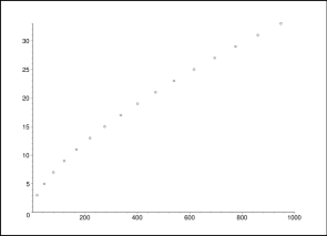
Figure 7: Plots of the zero modes for $p=1,3,5$ (left), and intersection points with $f(z)=z^{-1/2},$ which is shown as the dashed line. We also plot (right) the intersection points between the zero modes and the function $f(z)=z^{-1/2}$ for several values of $p.$

Let us now comment a little further on the 2-kink solutions that we have found in Eq. (10). We can have a better view of these defect structures calculating ${\widetilde{y}}_{p}$, the position which identifies the center of the defect. We identify ${\widetilde{y}}_{p}$ with the maxima of the derivative of the defect solutions, that is, ${\widetilde{y}}_{p}=\max[d\phi_{p}(y)/dy].$ We get ${\widetilde{y}}_{p}=\pm p\,{\rm arctanh}\,\sqrt{(p-1)/(p+1)}.$ For $p=1$ it gives ${\bar{y}}_{1}=0,$ as expected, but for $p=3,5,...,$ we obtain two non-zero values, which are directly related to the center of the interfaces that inhabits the defect. In flat spacetime, the values ${\widetilde{y}}_{p}$ exactly identify the maxima of the energy density

$${\widetilde{T}}^{p}_{00}(y)=\frac{1}{2}\left(\frac{d\phi_{p}}{dy}\right)^{2}+\frac{1}{2}\left(\frac{1}{2}\frac{dW_{p}}{d\phi}\right)^{2}$$ (19)

for the corresponding solutions $\phi_{p}(y)$ — the unusual $1/2$ factor that multiplies $W_{p}$ appears because in flat spacetime we have to redefine $W_{p}$ as $W_{p}/2,$ in order not to change the first-order equation (8) for the scalar field $\phi.$ This result shows that the 2-kink solutions are composed of two interfaces, each one being centered at each one of the two points ${\widetilde{y}}_{p}$ that we have just obtained. In curved spacetime, however, the position of the maxima of the matter energy density is different. To see this, we use $T^{p}_{00}(y)$ to identify the maxima of the matter energy density in curved spacetime. The function $T^{p}_{00}(y)$ is depicted in Fig. [4] for some values of $p.$ There are maxima at the points $y_{3}=2.42,\,y_{5}=5.36,\,y_{7}=8.70,...,$ which are different from the points ${\widetilde{y}}_{3}=2.64,\,{\widetilde{y}}_{5}=5.73,\,{\widetilde{y}}_{7}=9.22,...,$ which identify the maxima of the energy density in flat spacetime, or the center of the interfaces of the 2-kink solutions that we have already found. This result leads to the conclusion that the curved spacetime induces an attraction between the interfaces that appear from the 2-kink solutions. We have investigated this effect for several $p$, and we could verify that the relative attraction decreases for increasing $p.$

We recall that solutions similar to the 2-kink defects depicted in Fig. [2] have already been considered before in flat spacetime. See for instance Ref. [10], which investigates a model described by a complex scalar field. We can also deal with two real scalar fields and consider the model investigated in [21] in flat spacetime. It is defined by $W(\phi,\chi)=\phi-\phi^{3}/3-r\phi\chi^{2},$ where $r$ is a real parameter. It supports kink-like solutions [22, 23] of the form presented in Fig. [2]. This model was very recently used to describe matter coupled to gravity in warped geometry [24], with the result that the warp factor resembles the form depicted in Fig. [3]. The models investigated in the present work are similar but simpler, since they are described by a single real scalar field.

The model investigated in [21] support two-field solutions in the sector defined by the minima $(\pm 1,0)$ in the $(\phi,\chi)$ plane [25]. We may couple this model to gravity, to investigate whether these two-field solutions generate braneworld scenarios. Other extensions may involve scalar fields described under the general guidance of the $Z_{2}\times Z_{3}$ symmetry — see for instance the second work in Ref. [25] — and they may also lead to issues involving branes that host network of non trivial structure.

We would like to thank F.A. Brito and J.R. Nascimento for helpful discussions. We also thank PROCAD and PRONEX for financial support. DB and CF thank CNPq for partial support and ARG thanks FAPEMA for a fellowship.

References

- [1] N. Arkani-Hamed, S. Dimopoulos, G. Dvali, Phys. Lett. B 429, (1998); I. Antoniadis, N. Arkani-Hamed, S. Dimopoulos, G. Dvali, Phys. Lett. B 436, 257 (1998).
- [2] L. Randall and R. Sundrum, Phys. Rev. Lett. 83, 3370 (1999); 83, 4690 (1999).
- [3] W.D. Goldberger and M.B. Wise, Phys. Rev. Lett. 83, 4922 (1999).
- [4] J. Garriga and T. Tanaka, Phys. Rev. Lett. 84, 2778 (2000).
- [5] R. Gregory, V.A. Rubakov, and S.M. Sibiryakov, Phys. Rev. Lett. 84, 5928 (2000).
- [6] O. DeWolfe, D.Z. Freedman, S.S. Gubser, and A. Karch, Phys. Rev. D 62, 046008 (2000).
- [7] M. Gremm, Phys. Lett. B 478, 434 (2000).
- [8] C. Csáki, J. Erlich, T.J. Hollowood, and Y. Shirman, Nucl. Phys. B 581, 309 (2000); C. Csáki, J. Erlich, C. Grojean, and T.J. Hollowood, Nucl. Phys. B 584, 359 (2000).
- [9] A. Campos, Phys. Rev. Lett. 88, 141602 (2002).
- [10] A. Campos, K. Holland and U.-J. Wiese, Phys. Rev. Lett. 81, 2420 (1998); Phys. Lett. B 443, 338 (1998).
- [11] D. Bazeia, J. Menezes, and R. Menezes, Phys. Rev. Lett. 91, 241601 (2003).
- [12] J.R. Morris, Phys. Rev. D 51, 697 (1995); Int. J. Mod. Phys. A 13, 1115 (1998).
- [13] D. Bazeia, R.F. Ribeiro, and M.M. Santos, Phys. Rev. D 54, 1852 (1996); J.D. Edelstein, M.L. Trobo, F.A. Brito and D. Bazeia, Phys. Rev. D 57, 7561 (1998); D. Bazeia, F.A. Brito, and H. Boschi-Filho, J. High Energy Phys. 04, 028 (1999).
- [14] R. Gregory and A. Padilla, Phys. Rev. D 65, 084013 (2002); Class. Quant. Grav. 19, 279 (2002).
- [15] D. Bazeia, L. Losano, and J.M.C. Malbouisson, Phys. Rev. D 66, 101701(R) (2002).
- [16] F.A. Brito, M. Cvetic, and S.C. Yoon, Phys. Rev. D 64, 064021 (2001).
- [17] M. Cvetic and N.D. Lambert, Phys. Lett. B 540, 301 (2003)
- [18] D. Bazeia, F.A. Brito, and J.R. Nascimento, Phys. Rev. D 68, 085007 (2003).
- [19] M. Cvetic, S. Griffies, and S. Rey, Nucl. Phys. B 381, 301 (1992).
- [20] K. Skenderis and P.K. Townsend, Phys. Let. B 468, 46 (1999).
- [21] D. Bazeia, M.J. dos Santos, and R.F. Ribeiro, Phys. Lett. A 208, 84 (1995); D. Bazeia, J.R. Nascimento, R.F. Ribeiro, and D. Toledo, J. Phys. A 30, 8157 (1997).
- [22] M.A. Shifman and M.B. Voloshin, Phys. Rev. D 57, 2590 (1998).
- [23] A. Alonso Izquierdo, M.A. González León, and J. Mateos Guilarte, Phys. Rev. D 65, 085012 (2002).
- [24] M. Eto and N. Sakai, Solvable models of domain walls in N=1 supergravity. hep-th/0307276.
- [25] D. Bazeia and F.A. Brito, Phys. Rev. D 61, 105019 (2000); 62, 101701(R) (2000).