SLAC-PUB-10090        
Chiral rings and GSO projection in Orbifolds

Abstract

The GSO projection in the twisted sector of orbifold background is sometimes subtle and incompatible descriptions are found in literatures. Here, from the equivalence of partition functions in NSR and GS formalisms, we give a simple rule of GSO projection for the chiral rings of string theory in ${\mathbb{C}}^{r}/{\mathbb{Z}}_{n}$, $r=1,2,3$. Necessary constructions of chiral rings are given by explicit mode analysis.

1 Introduction

Recent study of closed string tachyon analysis[1, 2, 3, 4, 5] raised the interests in the string theory in non-compact orbifold backgrounds. The essential ingredient in either chiral ring technique[3] or mirror symmetry approach[2, 7, 8] is the world sheet ${\cal N}=2$ supersymmetry of NSR formalism, which in turn requires a precise understanding of the GSO projection. However, the description of this basic ingredient is rather subtle and the subtlety comes from following reason: in untwisted string theory, the criteria is the spacetime supersymetry which fixes a ${\mathbb{Z}}_{2}$ projection unambiguously. However, in orbifold theory, the spacetime SUSY is broken even after we impose a GSO projection and the imposition of SUSY in untwisted sector does not fix the action of ${\mathbb{Z}}_{2}$ projection in the twisted sector uniquely, in the sense that there are many ways of defining ${\mathbb{Z}}_{2}$ operartion. Hence the choice of GSO is largely arbitrary and in fact it is not hard to find that descriptions in literatures are partially incompatible with one another. Furthermore it is not clear whether such GSO projection rules give string theories equivalent to those in Green-Schwarz formalism.

In this paper, we explicitly work out the chiral rings and GSO projection rules on them for non-compact orbifolds ${\mathbb{C}}^{r}/{\mathbb{Z}}_{n}$, $r=3$ such that it guarantee the equivalence of the NSR and Green-Schwarz formalisms. We find that GS-NSR equivalence uniquely fixes a GSO for all twisted sectors and gives us a simple rule for the GSO projection. For $r=1,2$, the same GSO rule was given in the paper [5].

The rest paper is as follows: After constructing the chiral ring by mode analysis in section 2, we derive the GSO rule in section 3 by looking at the low temperature limits of partition function. We derive partition functions of NSR formalism starting from that of Green-Schwarz one using the Riemann’s theta identities. The spectrum analysis from this partition function gives the surviving condition of individual energy values, which we identify as the rule of the GSO projection.

2 Construction of Chiral Rings of ${\mathbb{C}}^{r}/{\mathbb{Z}}_{n}$

The purpose of this section is to explicitly construct the chiral rings of orbifold theories[6], which is essential both in language and in physical interpretation of section 3. We use mode analysis and rewrite the result in terms of monomials of mirror Landau-Ginzburg picture [2], whose review is not included here.

2.1 ${\mathbb{C}}^{1}/{\mathbb{Z}}_{n}$

The Energy momentum tensor of the NSR string on the cone ${\mathbb{C}}^{1}/{\mathbb{Z}}_{n}$ is

$$T=-\partial X{\partial}X^{*}+{1\over 2}\psi^{*}\partial\psi+{1\over 2}\psi\partial\psi^{*},$$ (2.1)

where $X=X^{1}+iX^{2},\;X^{*}=X^{1}-iX^{2}$ and $\psi$ and $\psi^{*}$ are Weyl fermions which are conjugate to each other with respect to the target space complex structure. All the fields appearing here describe worldsheet left movers. We denote the corresponding worldsheet complex conjugate by barred fields: ${\bar{X}},{\bar{X}^{*}},{\bar{\psi}},{\bar{\psi}^{*}}$. The ${\cal N}=2$ world sheet SCFT algebra is generated by $T$, $G^{+}=\psi^{*}\partial X$, $G^{-}=\psi\partial X^{*}$ and $J=\psi^{*}\psi$. The orbifold symmetry group

$${\mathbb{Z}}_{n}=\{g^{l}|l=0,1,2,\cdots,n-1,{\rm with}\;\;g^{n}=1\}$$ (2.2)

act on the fields in NS sector by

$$g\cdot X(\sigma+2\pi,\tau) = e^{2\pi ik/n}g\cdot X(\sigma,\tau),\;\;$$

$$g\cdot X^{*}(\sigma+2\pi,\tau) = e^{-2\pi ik/n}g\cdot X^{*}(\sigma,\tau),$$

$$g\cdot\psi(\sigma+2\pi,\tau) = -e^{2\pi ik/n}g\cdot\psi(\sigma,\tau),\;\;$$

$$g\cdot\psi^{*}(\sigma+2\pi,\tau) = -e^{-2\pi ik/n}g\cdot\psi^{*}(\sigma,\tau).$$ (2.3)

The mode expansions of the the fields in the conformal plane are given by

$$\partial X(z)= \sum_{n\in{\mathbb{Z}}}\alpha_{n+a}/z^{n+1+a},\;$$

$$\partial X^{*}(z)= \sum_{n\in{\mathbb{Z}}}\alpha^{*}_{n-a}/z^{n+1-a},\;$$

$$\psi(z)= \sum_{r\in{\mathbb{Z}}+{1\over 2}}\psi_{r+a}/z^{r+{1\over 2}+a},\;$$

$$\psi^{*}(z)= \sum_{r\in{\mathbb{Z}}+{1\over 2}}\psi^{*}_{r-a}/z^{r+{1\over 2}-a},$$ (2.4)

where $a=k/n$. The quantization conditions are:

$$[\alpha_{n+a},\alpha^{*}_{-m-a}]=(n+a)\delta_{m,n},\quad\{\psi_{r+a},\psi^{*}_{-s-a}\}=\delta_{r,s}.$$ (2.5)

Hence the conjugate variables are given by

$$\alpha^{\dagger}_{n+a}=\alpha^{*}_{-n-a}, \;(\alpha^{*}_{n-a})^{\dagger}=\alpha_{-n+a},\;$$

$$\psi^{\dagger}_{r+a}=\psi^{*}_{-r-a}, (\psi^{*}_{r-a})^{\dagger}=\psi_{-r+a}.$$ (2.6)

The vacuum is defined as a state that is annihilated by all positive modes. Notice that as $a$ grows greater than ${1\over 2}$, $\psi_{-{1\over 2}+a}$ ($\psi^{*}_{{1\over 2}-a}$)changes from a creation(annihilation) to an annihilation (creation) operator. The (left mode) hamiltonian of the orbifolded complex plane is

$$H_{L}={1\over 2}\sum\left[\alpha^{*}_{-n-a}\alpha_{n+a}+\alpha_{-n+a}\alpha^{*}_{n-a}\right]+{1\over 2}\sum_{r\in{\mathbb{Z}}+{1\over 2}}\left[(r+a)\psi^{*}_{-r-a}\psi_{r+a}+(r-a)\psi_{-r+a}\psi^{*}_{n-a}\right].$$ (2.7)

The contribution of the left modes to the zero energy is

$$E_{0}^{L}={1\over 2}\sum_{n=0}^{\infty}(n+a)+{1\over 2}\sum_{n=1}^{\infty}(n-a)-{1\over 2}\sum_{n=0}^{\infty}(n+{1\over 2}+a)-{1\over 2}\sum_{n=0}^{\infty}({1\over 2}+n-a).$$ (2.8)

If we define

$$f(a)=\sum_{n=0}^{\infty}(n+a)=1/24-(a-1/2)^{2}/2,$$ (2.9)

then $f(a)=f(1-a)$ and $f(a+1/2)=f(-a+1/2)$ so that the above sum gives $E_{0}^{L}=a/2-1/8$. Embedding the cone to the string theory to make the target space ${\mathbb{C}}/{\mathbb{Z}}_{n}\times R^{7,1}$, we need to add the zero energy fluctuation of the 6 transverse flat space, $6\times(-1/24)(1+1/2)=-3/8$ to the zero point energy, which finally become

$$E_{0}^{L}={1\over 2}(a-1),\quad for\quad 0<a<{1\over 2}.$$ (2.10)

If $1/2<a<1$, then $(a-{1\over 2})\psi^{*}_{{1\over 2}-a}\psi_{-{1\over 2}+a}$ should be added to the normal ordered Hamiltonian while $({1\over 2}-a)\psi_{-{1\over 2}+a}\psi^{*}_{{1\over 2}-a}$ should be removed from it. Therefore the zero point energy should be modified to be

$$E_{0}^{L}={1\over 2}\left(a-1\right)-{1\over 2}\left[-\left({1\over 2}-a\right)+\left(a-{1\over 2}\right)\right]=-{1\over 2}a,\quad for\quad{1\over 2}<a<1.$$ (2.11)

From this we can identify the weight and charge of twisted ground states using

$$E_{0}^{L}=\Delta-1/2,\quad{\rm and}\quad q=\pm 2\Delta,$$ (2.12)

where we take + if the the ground state is a chiral state and $-$ if it is anti-chiral state.

We now construct next level chiral and anti-chiral primary states by applying the creation operator.

$$G^{+}_{-{1\over 2}} = \sum\psi^{*}_{-n-{1\over 2}-a}\alpha_{n+a}=\psi^{*}_{{1\over 2}-a}\alpha_{-1+a}+\cdots,\;$$

$$G^{-}_{-{1\over 2}} = \sum\psi_{-n-{1\over 2}+a}\alpha^{*}_{n-a}=\psi_{-{1\over 2}+a}\alpha^{*}_{-a}+\cdots.$$ (2.13)

Notice that for $0<a<{1\over 2}$, $\psi^{*}_{{1\over 2}-a}|0>=0$, hence

$$G^{+}_{-{1\over 2}}|0>=0$$ (2.14)

so that $|0>$ is a chiral state. It has a weight $a/2$ and a R-charge $a$, so that the local ring element of LG theory corresponding to $|0>_{a}$ can be identified as $u^{k}$:

$$|0>_{a}\sim u^{k}.$$ (2.15)

The first excited state is $\psi_{a-{1\over 2}}|0>$ which is annihilated by $G^{-}_{-{1\over 2}}$:

$$G^{-}_{-{1\over 2}}\psi_{a-{1\over 2}}|0>=0.$$ (2.16)

Therefore it is an anti-chiral state. Its weight is ${1\over 2}(1-a)$ and charge is $a-1$, hence it corresponds to ${\bar{u}}^{n-k}$:

$$\psi_{a-{1\over 2}}|0>\sim{\bar{u}}^{n-k}.$$ (2.17)

For ${1\over 2}<a<1$, $\psi_{a-{1\over 2}}|0>=0$, hence $G^{-}_{-{1\over 2}}|0>=0$ so that $|0>$ is an anti-chiral state. It has weight ${1\over 2}(1-a)$ and charge $a-1$, hence the corresponding local ring element is ${\bar{u}}^{n-k}$. The first excited state is $\psi^{*}_{{1\over 2}-a}|0>$ which is annihilated by $G^{+}_{-{1\over 2}}$ therefore it is a chiral state. Its weight is $a/2$ and the charge is $a$ hence the corresponding local ring element is again $u^{k}$. Using the weight and charge relation for chiral and anti-chiral states, we see that $\psi^{*}$ has $+1$ charge and $\psi$ has $-1$ charge.

So far we have worked out the first twisted sector for arbitrary generator $k$. For the $j$-th twisted sector, we can easily extend the above identifications by observing that $a$ is the fractional part of $jk/n$;

$$a=\{jk/n\}.$$ (2.18)

The result is that for all chiral operators, the local ring elements are given by $u^{n\{jk/n\}}$ and for the anti-chiral operators they are given by ${\bar{u}}^{n-n\{jk/n\}}$. In both cases $j$ runs from 1 to $n-1$ for twisted sectors. It is worthwhile to observe that

$$n(1-\{jk/n\})=n\{j(n-k)/n\},$$ (2.19)

so that the generator of the anti-chiral ring is ${\bar{u}}^{n-k}$, while that of chiral ring is ${u}^{k}$. Since it is the building block for the results in higher dimensional theories, we tabulate the above results in Table 1.

Region	vacuum	annihilator	creators
$0<a<{1\over 2}$	$|0>\sim u^{na}$	$\psi^{*}_{{1\over 2}-a}$	$\psi_{a-{1\over 2}}|0>\sim{\bar{u}}^{n-na}$
${1\over 2}<a<1$	$|0>\sim{\bar{u}}^{n-na}$	$\psi_{a-{1\over 2}}$	$\psi^{*}_{{1\over 2}-a}|0>\sim{u}^{na}$

Table 1: Twisted vacuum and first excited states. The chirality is equal to the holomorphic structure of the target space, i.e, chiral(anti-chiral) states correspond to monomial of $u$ ($\bar{u}$).

What about the case $a=-k/n<0$ The answer can be read off from what we already have by noticing that above structure is periodic in $a$ with period 1, because we should shift the mode if $a$ is bigger than 1. The effect of $a\to-a$ amounts to exchanging the role of $\psi$ and $\psi^{*}$. Therefore in this case, the local ring elements of LG dual are given by $u^{n-n\{jk/n\}}$ and for the anti-chiral operators they are given by ${\bar{u}}^{n\{jk/n\}}$.

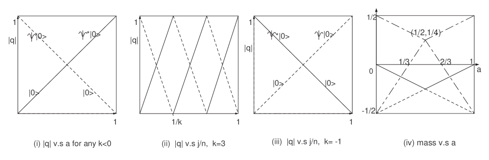
Figure 1: Spectrum versus twists in ${\mathbb{C}}^{1}/{\mathbb{Z}}_{n}$: (i) $2\Delta=|q|$ v.s $a=\{jk/n\}$ for any $k>0$. The states on solid lines are chiral while those on the dotted lines are anti-chiral. (ii) $|q|$ v.s $j/n$ for k=3, (iii) $|q|$ v.s $j/n$ for $k=-1$. For $k<0$, the role of chiral and anti-chiral states are interchanged. (iv) All possible Tachyom mass v.s $a$. Dotted lines are for the (twisted) vacuum, solid lines are for worldsheet fermion excitations, the rests are for scalar excitations. Notice that the lowest tachyon mass is always generated by worldsheet fermion.

The first three graphs in Fig.1 show the weight versus twist $a$ for the various cases. The charge can be read off by the $q=\pm 2\Delta$ rule. We are interested in $2\Delta$ since left and right moving parts contribute the same to the masses of the states represented by these polynomials. The last figure in Fig.1 is mass spectrum $\frac{1}{4}\alpha^{\prime}M^{2}=E_{0}^{L}$ as a function of the twist $a$ for all possible tachyons including the scalar excitations:

$$\alpha^{*}_{-a}|0\rangle:\;E_{0}^{L}= (3a-1)/2,\;{\rm for}\; 0<a<{1\over 2}$$

$$= {a}/{2},\;\;\;{\rm for}\; {1\over 2}<a<1$$

$$\alpha_{-(1-a)}|0\rangle:\;E_{0}^{L}= (1-a)/,\;{\rm for}\; 0<a<{1\over 2}$$

$$= {(2-3a)}/{2},\;{\rm for}\; {1\over 2}<a<1.$$ (2.20)

These scalar excitations $\alpha^{*}_{-a}|0\rangle,\alpha_{-(1-a)}|0\rangle$ are tachyons if $0<a<1/3$, $2/3<a<1$ respectively. They can not be characterized as chiral or anti-chiral states. Furthermore it never gives the lowest tachyon mass, hence we will not pay much attention afterward.

2.2 ${\mathbb{C}}^{2}/{\mathbb{Z}}_{n}$

Now we extend the result of previous section to ${\mathbb{C}}^{2}/{\mathbb{Z}}_{n}$ case, which is our main interests. We introduce two sets of (bosonic and fermionic) complex fields $X^{(1)},\psi^{(1)},\psi^{*(1)};$ $X^{(2)},X^{*(2)},\psi^{(2)},\psi^{*(2)}$ and specify how the orbifold group ${\mathbb{Z}}_{n}$ is acting on each set of fields. The group action is the same as before except that ${\mathbb{Z}}_{n}$ can act on first and second set of fields with different generators $k_{1}$ and $k_{2}$. For example, in the first twisted sector,

$$g\cdot X^{(j)}(\sigma+2\pi,\tau)=e^{2\pi ik_{j}/n}g\cdot X^{(j)}(\sigma,\tau),\quad for\quad j=1,2.$$ (2.21)

Since three parameter $n,k_{1},k_{2}$ fix an ${\mathbb{C}}^{2}/{\mathbb{Z}}_{n}$ orbifold theory completely, we use notation $n(k_{1},k_{2})$ to denote it.

Let $a_{i}=k_{i}/n$ as before. For $0<a_{i}<{1\over 2}$, the zero energy fluctuation can be calculated as

$$E_{0}^{L}=\left({1\over 2}a_{1}-\frac{1}{8}\right)+\left({1\over 2}a_{2}-\frac{1}{8}\right)-\frac{1}{24}\left(1+{1\over 2}\right)\times 4={1\over 2}\left(a_{1}+a_{2}-1\right).$$ (2.22)

Therefore the weight of twisted vacuum is given by

$$\Delta_{0}={1\over 2}(a_{1}+a_{2}).$$ (2.23)

We define

$$G^{+}=G_{1}^{+}+G_{2}^{+},$$ (2.24)

where $G_{i}^{+}=\psi^{*(i)}\partial X^{(i)}$. For abbreviation, we use following notations;

$$\psi_{i}:=\psi^{(i)}_{a_{i}-{1\over 2}}\quad{\rm and}\;\;\psi_{i}^{*}:=\psi^{*(i)}_{{1\over 2}-a_{i}}.$$ (2.25)

Then for $a_{1}<{1\over 2},a_{2}<{1\over 2}$, we have $\psi^{*}_{1}|0>=0$ and $\psi_{2}^{*}|0>=0$, which gives $G^{+}_{-{1\over 2}}|0>=0$ so that the twisted vacuum is a chiral state, whose associated local ring element is identified:

$$|0>\sim u_{1}^{n\{jk_{1}/n\}}u_{2}^{n\{jk_{2}/n\}}.$$ (2.26)

Both $\psi_{1},\psi_{2}$ are creation operators and $G^{-}_{-{1\over 2}}\psi_{1}\psi_{2}|0>=0$, so that $\psi_{1}\psi_{2}|0>$ is an anti-chiral state. By considering weight and charge, corresponding monomial is found to be

$$\psi_{1}\psi_{2}|0>\sim{\bar{u}_{1}}^{n-n\{jk_{1}/n\}}{\bar{u}_{2}}^{n-n\{jk_{2}/n\}}.$$ (2.27)

So far, $\psi^{*}_{i}|0>$’s are neither chiral($c$) nor anti-chiral($a$). One can work out other three cases in similar fashion. We summarize the result in the Table 2.

($a_{1}-{1\over 2}$,$a_{2}-{1\over 2}$)	$b$	$b^{\dagger}$	chiral state	anti-chiral state	neither
$--$	$\psi^{*}_{1},\psi_{2}^{*}$	$\psi_{1},\psi_{2}$	$|0>$	$\psi_{1}\psi_{2}|0>$	$\psi_{1}|0>\sim{\bar{u}_{1}}^{n-na_{1}}u_{2}^{na_{2}}$
			$\sim u_{1}^{na_{1}}u_{2}^{na_{2}}$	$\sim{\bar{u}_{1}}^{n-na_{1}}{\bar{u}_{2}}^{n-na_{2}}$	$\psi_{2}|0>\sim{u_{1}}^{na_{1}}{\bar{u}}_{2}^{n-na_{2}}$
$-+$	$\psi^{*}_{1},\psi_{2}$	$\psi_{1},\psi^{*}_{2}$	$\psi_{2}^{*}|0>$	$\psi_{1}|0>$	$|0>\sim{u_{1}}^{na_{1}}{\bar{u}}_{2}^{n-na_{2}}$
			$\sim u_{1}^{na_{1}}u_{2}^{na_{2}}$	$\sim{\bar{u}_{1}}^{n-na_{1}}{\bar{u}_{2}}^{n-na_{2}}$	$\psi_{1}\psi_{2}^{*}|0>\sim{\bar{u}_{1}}^{n-na_{1}}u_{2}^{na_{2}}$
$+-$	$\psi_{1},\psi_{2}^{*}$	$\psi^{*}_{1},\psi_{2}$	$\psi_{1}^{*}|0>$	$\psi_{2}|0>$	$|0>\sim{\bar{u}_{1}}^{n-na_{1}}u_{2}^{na_{2}}$
			$\sim u_{1}^{na_{1}}u_{2}^{na_{2}}$	$\sim{\bar{u}_{1}}^{n-na_{1}}{\bar{u}_{2}}^{n-na_{2}}$	$\psi^{*}_{1}\psi_{2}|0>\sim{u_{1}}^{na_{1}}{\bar{u}}_{2}^{n-na_{2}}$
$++$	$\psi_{1},\psi_{2}$	$\psi^{*}_{1},\psi^{*}_{2}$	$\psi_{1}^{*}\psi_{2}^{*}|0>$	$|0>$	$\psi^{*}_{1}|0>\sim{u_{1}}^{na_{1}}{\bar{u}}_{2}^{n-na_{2}}$
			$\sim u_{1}^{na_{1}}u_{2}^{na_{2}}$	$\sim{\bar{u}_{1}}^{n-na_{1}}{\bar{u}_{2}}^{n-na_{2}}$	$\psi^{*}_{2}|0>\sim{\bar{u}_{1}}^{n-na_{1}}u_{2}^{na_{2}}$

Table 2: Oscillator and monomial representations of chiral and anti-chiral rings. $+-$ means ($a_{1}-{1\over 2})>0,(a_{2}-{1\over 2})<0$.

Notice that (anti-)chiral states in different parameter ranges have different oscillator representations but have the same polynomial expressions as local ring elements.

When some of $a_{i}<0$, one can get the similar result by exchanging the role of $\psi$ and $\psi^{*}$, and $u_{i}$ and ${\bar{u}}_{i}$. As a result, for the factor with the negative twist $a_{i}=-\{jk_{i}/n\}$, we need to use $u_{i}^{n-n\{jk_{i}/n\}}$ for the chiral states and ${\bar{u}_{i}}^{n\{jk_{i}/n\}}$ for the anti-chiral states, while for the factor with the positive twist $\{jk_{i}/n\}$, we need to use $u_{i}^{n\{jk_{i}/n\}}$ for the chiral states and ${\bar{u}_{i}}^{n\{jk_{i}/n\}}$ for the anti-chiral states. For example: if only $a_{2}$ is negative, the chiral states are associated with $u_{1}^{n\{jk_{1}/n\}}u_{2}^{n-n\{jk_{2}/n\}}$, while the anti-chiral states are associated with ${\bar{u}_{1}}^{n-n\{jk_{1}/n\}}{\bar{u}_{2}}^{n\{jk_{2}/n\}}$. We summarize the result in the Table 3.

$(a_{1},a_{2})$	$c$-ring	$2\Delta$	$a$-ring	$2\Delta$
$++$	$u_{1}^{na_{1}}u_{2}^{na_{2}}$	$a_{1}+a_{2}$	${\bar{u}_{1}}^{n(1-a_{1})}{\bar{u}_{2}}^{n(1-a_{2})}$	$2-a_{1}-a_{2}$
$+-$	$u_{1}^{na_{1}}u_{2}^{n(1-|a_{2}|)}$	$a_{1}-|a_{2}|+1$	${\bar{u}_{1}}^{n(1-a_{1})}{\bar{u}_{2}}^{n|a_{2}|}$	$1-a_{1}+|a_{2}|$
$-+$	$u_{1}^{n(1-|a_{1}|)}u_{2}^{na_{2}}$	$1-|a_{1}|+a_{2}$	${\bar{u}_{1}}^{n|a_{1}|}{\bar{u}_{2}}^{n(1-a_{2})}$	$|a_{1}|-a_{2}+1$
$--$	$u_{1}^{n(1-|a_{1}|)}u_{2}^{n(1-|a_{2}|)}$	$2-|a_{1}|-|a_{2}|$	${\bar{u}_{1}}^{n|a_{1}|}{\bar{u}_{2}}^{n|a_{2}|}$	$|a_{1}|+|a_{2}|$

Table 3: Monomial basis of chiral and anti-chiral rings and their weights when some of $a_{i}$ is negative. $+-$ means $a_{1}>0,a_{2}<0$. The R-charges can be read off by the rule $q=\pm 2\Delta$.

2.3 ${\mathbb{C}}^{3}/{\mathbb{Z}}_{n}$

Now let $a_{i}=k_{i}/n$ as before with $i=1,2,3$ and consider first $0<a_{i}<{1\over 2}$. The zero energy fluctuation can be calculated as

$$E_{0}^{L}=\sum_{i}({1\over 2}a_{i}-{1\over 8})-{1\over 24}(1+{1\over 2})\times 2={1\over 2}(a_{1}+a_{2}+a_{3}-1).$$ (2.28)

Hence the weight of the twisted vacuum can be read off as before

$$\Delta_{0}={1\over 2}(a_{1}+a_{2}+a_{3}).$$ (2.29)

We define

$$G^{+}=G^{+}_{1}+G^{+}_{2}+G^{+}_{3},$$ (2.30)

where $G^{+}_{i}=\psi^{*(i)}\partial X^{(i)}$. For abbreviation we use the following notations

$$\psi_{i}:=\psi^{(i)}_{a_{i}-{1\over 2}}\;\;\;\;\;\psi^{*}_{i}:=\psi^{*(i)}_{{1\over 2}-a_{i}}.$$ (2.31)

Suppose $a_{i}<{1\over 2}$ then

$$\psi^{*}_{i}|0>=0\quad i.e.\quad G^{+}_{-{1\over 2}}|0>=0.$$ (2.32)

Thus the twisted vacuum is a chiral state, in other words

$$|0>\sim u_{1}^{n\{{jk_{1}/n}\}}u_{2}^{n\{jk_{2}/n\}}u_{3}^{n\{jk_{3}/n\}},$$ (2.33)

while

$$G^{-}_{-{1\over 2}}\psi_{1}\psi_{2}\psi_{3}|0>=0,$$ (2.34)

meaning

$$\psi_{1}\psi_{2}\psi_{3}|0>\sim\bar{u}_{1}^{n-n\{jk_{1}/n\}}\bar{u}_{2}^{n-n\{jk_{2}/n\}}\bar{u}_{3}^{n-n\{jk_{3}/n\}}.$$ (2.35)

is an anti-chiral state. We summarize this in Table 4 and for $a_{i}<0$ in Table 5.

$(a_{1}-{1\over 2},a_{2}-{1\over 2},a_{3}-{1\over 2})$	$b$	$b^{\dagger}$	chiral	anti-chiral
$(-,-,-)$	$\psi^{*}_{1},\psi^{*}_{2},\psi^{*}_{3}$	$\psi_{1},\psi_{2},\psi_{3}$	$|0>$	$\psi_{1}\psi_{2}\psi_{3}|0>$
			$\sim u_{1}^{na_{1}}u_{2}^{na_{2}}u_{3}^{na_{3}}$	$\sim\bar{u}_{1}^{n-na_{1}}\bar{u}_{2}^{n-na_{2}}\bar{u}_{3}^{n-na_{3}}$
$(-,+,-)$	$\psi^{*}_{1},\psi_{2},\psi^{*}_{3}$	$\psi_{1},\psi^{*}_{2},\psi_{3}$	$\psi^{*}_{2}|0>$	$\psi_{1}|0>$
			$\sim u_{1}^{na_{1}}u_{2}^{na_{3}}u_{3}^{na_{3}}$	$\sim\bar{u}_{1}^{n-na_{1}}\bar{u}_{2}^{n-na_{2}}\bar{u}_{3}^{n-na_{3}}$
$(-,-,+)$	$\psi^{*}_{1},\psi^{*}_{2},\psi_{3}$	$\psi_{1},\psi_{2},\psi^{*}_{3}$	$\psi^{*}_{3}|0>$	$\psi_{1}\psi_{2}|0>$
			$\sim u_{1}^{na_{1}}u_{2}^{na_{2}}u_{3}^{na_{3}}$	$\sim\bar{u}_{1}^{n-na_{1}}\bar{u}_{2}^{n-nq_{2}}u_{3}^{n-na_{3}}$
$(+,-,-)$	$\psi_{1},\psi^{*}_{2},\psi^{*}_{3}$	$\psi^{*}_{1},\psi_{2},\psi_{3}$	$\psi^{*}_{1}|0>$	$\psi_{2}\psi_{3}|0>$
			$\sim u_{1}^{na_{1}}u_{2}^{na_{2}}u_{3}^{na_{3}}$	$\sim\bar{u}_{1}^{n-na_{1}}\bar{u}_{2}^{n-na_{2}}\bar{u}_{3}^{n-na_{3}}$
$(+,+,-)$	$\psi_{1},\psi_{2},\psi^{*}_{3}$	$\psi^{*}_{1},\psi^{*}_{2},\psi_{3}$	$\psi^{*}_{1}\psi^{*}_{2}|0>$	$\psi_{3}|0>$
			$\sim u_{1}^{na_{1}}u_{2}^{na_{2}}u_{3}^{na_{3}}$	$\sim\bar{u}_{1}^{n-na_{1}}\bar{u}_{2}^{n-na_{2}}\bar{u}_{3}^{n-na_{3}}$
$(+,-,+)$	$\psi_{1},\psi^{*}_{2},\psi_{3}$	$\psi^{*}_{1},\psi_{2},\psi^{*}_{3}$	$\psi^{*}_{1},\psi^{*}_{3}|0>$	$\psi_{2}|0>$
			$\sim u_{1}^{na_{1}}u_{2}^{na_{2}}u_{3}^{na_{3}}$	$\sim\bar{u}_{1}^{n-na_{1}}\bar{u}_{2}^{n-na_{2}}\bar{u}_{3}^{n-na_{3}}$
$(-,+,+)$	$\psi^{*}_{1},\psi_{2},\psi_{3}$	$\psi_{1},\psi^{*}_{2},\psi^{*}_{3}$	$\psi^{*}_{2}\psi^{*}_{3}|0>$	$\psi_{1}|0>$
			$\sim u_{1}^{na_{1}}u_{2}^{na_{2}}u_{3}^{na_{3}}$	$\sim\bar{u}_{1}^{n-na_{1}}\bar{u}_{2}^{n-na_{2}}\bar{u}_{3}^{n-na_{3}}$
$(+,+,+)$	$\psi_{1},\psi_{2},\psi_{3}$	$\psi^{*}_{1},\psi^{*}_{2},\psi^{*}_{3}$	$\psi^{*}_{1}\psi^{*}_{2}\psi^{*}_{3}|0>$	$|0>$
			$\sim u_{1}^{na_{1}}u_{2}^{na_{2}}u_{3}^{na_{3}}$	$\sim\bar{u}_{1}^{n-na_{1}}\bar{u}_{2}^{n-na_{2}}\bar{u}_{3}^{n-na_{3}}$

Table 4: Oscillator and monomial representations of chita and anti-chiral rings: $-(+)$ means $a_{i}<{1\over 2}(a_{i}>{1\over 2})$.

$a_{1}$, $a_{2}$, $a_{3}$	$c$-ring	2 $\Delta$	$a$-ring	2$\Delta$
$+,+,+$	$u_{1}^{na_{1}}u_{2}^{na_{2}}u_{3}^{na_{3}}$	$a_{1}+a_{2}+a_{3}$	$\bar{u}_{1}^{n(1-a_{1})}\bar{u}_{2}^{n(1-a_{2})}\bar{u}_{3}^{n(1-a_{3})}$	$3-a_{1}-a_{2}-a_{3}$
$+,-,+$	$u_{1}^{na_{1}}u_{2}^{n-n|a_{2}|}u_{3}^{na_{3}}$	$a_{1}+1-|a_{2}|+a_{3}$	$\bar{u}_{1}^{n(1-a_{1})}\bar{u}_{2}^{n|a_{2}|}\bar{u}_{3}^{n(1-a_{3})}$	$2-a_{1}+|a_{2}|-a_{3}$
$+,+,-$	$u_{1}^{na_{1}}u_{2}^{na_{2}}u_{3}^{n-n|a_{3}|}$	$a_{1}+a_{2}+1-|a_{3}|$	$\bar{u}_{1}^{n(1-a_{1})}\bar{u}_{2}^{n(1-a_{2})}\bar{u}_{3}^{n|a_{3}|}$	$2-a_{1}-a_{2}+|a_{3}|$
$-,+,+$	$u_{1}^{n-n|a_{1}|}u_{2}^{na_{2}}u_{3}^{na_{3}}$	$1-|a_{1}|+a_{2}+a_{3}$	$\bar{u}_{1}^{n|a_{1}|}\bar{u}_{2}^{n(1-a_{2})}\bar{u}_{3}^{n(1-a_{3})}$	$2+|a_{1}|-a_{2}-a_{3}$
$-,-,+$	$u_{1}^{n-n|a_{1}|}u_{2}^{n-n|a_{2}|}u_{3}^{na_{3}}$	$2-|a_{1}|-|a_{2}|+a_{3}$	$\bar{u}_{1}^{n|a_{1}|}\bar{u}_{2}^{n|a_{2}|}\bar{u}_{3}^{n(1-a_{3})}$	$1+|a_{1}|+|a_{2}|-a_{3}$
$-,+,-$	$u_{1}^{n-n|a_{1}|}u_{2}^{na_{2}}u_{3}^{n-n|a_{3}|}$	$2-|a_{1}|+a_{2}-|a_{3}|$	$\bar{u}_{1}^{n|a_{1}|}\bar{u}_{2}^{n(1-a_{2})}\bar{u}_{3}^{n|a_{3}|}$	$1+|a_{1}|-a_{2}+|a_{3}|$
$+,-,-$	$u_{1}^{na_{1}}u_{2}^{n-n|a_{2}|}u_{3}^{n-n|a_{3}|}$	$2+a_{1}-|a_{2}|-|a_{3}|$	$\bar{u}_{1}^{n(1-a_{1})}\bar{u}_{2}^{n|a_{2}|}\bar{u}_{3}^{n|a_{3}|}$	$1-a_{1}+|a_{2}+|a_{3}|$
$-,-,-$	$u_{1}^{n-n|a_{1}|}u_{2}^{n-n|a_{2}|}u_{3}^{n-n|a_{3}|}$	$3-|a_{1}|-|a_{2}|-|a_{3}|$	$\bar{u}_{1}^{n|a_{1}|}\bar{u}_{2}^{n|a_{2}|}\bar{u}_{3}^{n|a_{3}|}$	$|a_{1}|+|a_{2}|+|a_{3}|$

Table 5: Monomial basis of chiral and anti-chiral rings and their weights when some of $a_{i}$ are negative.

$G$	c-ring	2 $\Delta$	$a$-ring	2$\Delta$
$G_{ccc}$	$u_{1}^{na_{1}}u_{2}^{na_{2}}u_{3}^{na_{3}}$	$a_{1}+a_{2}+a_{3}$	$\bar{u}_{1}^{n(1-a_{1})}{\bar{u}}_{2}^{n(1-q_{2})}\bar{u}_{3}^{n(1-a_{3})}$	$3-a_{1}-a_{2}-a_{3}$
$G_{cac}$	$u_{1}^{na_{1}}\bar{u}_{2}^{n-na_{2}}u_{3}^{na_{3}}$	$a_{1}+1-a_{2}+a_{3}$	$\bar{u}_{1}^{n(1-a_{1})}u_{2}^{na_{2}}\bar{u}_{3}^{n(1-a_{3})}$	$2-a_{1}+a_{2}-a_{3}$
$G_{cca}$	$u_{1}^{na_{1}}u_{2}^{na_{2}}\bar{u}_{3}^{n-na_{3}}$	$a_{1}+a_{2}+1-a_{3}$	$\bar{u}_{1}^{n(1-a_{1})}\bar{u}_{2}^{n(1-a_{2})}u_{3}^{na_{3}}$	$2-a_{1}-a_{2}+a_{3}$
$G_{acc}$	$\bar{u}_{1}^{n-na_{1}}u_{2}^{na_{2}}u_{3}^{na_{3}}$	$1-a_{1}+a_{2}+a_{3}$	$u_{1}^{na_{1}}\bar{u}_{1}^{n(1-a_{2})}\bar{u}_{3}^{n(1-a_{3})}$	$2+a_{1}-a_{2}-a_{3}$
$G_{aac}$	$\bar{u}_{1}^{n-na_{1}}\bar{u}_{2}^{n-na_{2}}u_{3}^{na_{3}}$	$2-a_{1}-a_{2}+a_{3}$	$u_{1}^{na_{1}}u_{2}^{na_{2}}\bar{u}_{3}^{n(1-a_{3})}$	$1+a_{1}+a_{2}-a_{3}$
$G_{aca}$	$\bar{u}_{1}^{n-na_{1}}u_{2}^{na_{2}}\bar{u}_{3}^{n-na_{3}}$	$2-a_{1}+a_{2}-a_{3}$	$u_{1}^{na_{1}}\bar{u}_{2}^{n(1-a_{2})}u_{3}^{na_{3}}$	$1+a_{1}-a_{2}+a_{3}$
$G_{caa}$	$u_{1}^{na_{1}}\bar{u}_{2}^{n-na_{2}}\bar{u}_{3}^{n-na_{3}}$	$2+a_{1}-a_{2}-a_{3}$	$\bar{u}_{1}^{n(1-a_{1})}u_{2}^{na_{2}}u_{3}^{na_{3}}$	$1-a_{1}+a_{2}+a_{3}$
$G_{aaa}$	$\bar{u}_{1}^{n-na_{1}}\bar{u}_{2}^{n-na_{2}}\bar{u}_{3}^{n-na_{3}}$	$3-a_{1}-a_{2}-a_{3}$	$u_{1}^{na_{1}}u_{2}^{na_{2}}u_{3}^{na_{3}}$	$a_{1}+a_{2}+a_{3}$

Table 6: Monomial basis of chiral and anti-chiral rings and their weights for varius choices of target space complex structures.

The discussion on the enhanced (2,2) SUSY can be described completely parallel way with ${\mathbb{C}}^{2}/{\mathbb{Z}}_{n}$ case.

3 GSO projection

3.1 Type 0 and type II Orbifold

Here we discuss when there is bulk tachyons whose presence/absence defines type 0/type II. Considering twist operation in Green-Schwarz formalism. We follow the argument in [1] and generalize it.

First we consider ${\mathbb{C}}^{1}/{\mathbb{Z}}_{n}$. Let $g$ be the orbifold action acting on complex plane;

$$g=e^{2\pi ikJ/n},\quad k=-n+1,\cdots,n-2,n-1,$$ (3.1)

where $J$ is the rotation generator in the complex plane that is orbifolded.

$$g^{n}=(-1)^{kF_{s}},$$ (3.2)

where $F_{s}$ means spacetime fermion number and we used $J=1/2$ for the spacetime fermion. Hence if $k$ is even, then $g^{n}=1$ and $g$ is a good generator of ${\mathbb{Z}}_{n}$ action. On the other hand, if $k$ is odd, $g^{n}=(-1)^{F_{s}}\neq 1$, and $g$ is not a generator of ${\mathbb{Z}}_{n}$ action. In fact $g$ is the generator of ${\mathbb{Z}}_{2n}$ action. The ${\mathbb{Z}}_{2n}$ projection operator $P$ projects out all spacetime fermion, since

$$P=\frac{1}{2n}\sum_{l=0}^{2n-1}g^{l}={1\over 2}(1+(-1)^{F_{s}})\cdot\sum_{l=0}^{n-1}g^{l}/n.$$ (3.3)

The consequence is type 0 string where there is no spacetime fermion. More precisely, the bulk fermion in untwisted sector is cancelled by those of $n$-th twisted sector.

In order to get type II string for $k$ odd case, one try to change the projection operator by

$$g^{\prime}=e^{2\pi ikJ/n}(-1)^{-2\pi iJ},$$ (3.4)

so that $g^{\prime n}=(-1)^{(k-n)F_{s}}$. Notice that under the change $g\to g^{\prime}$, it follows that $k\to k-n$ in eq.(3.1) and $k^{\prime}=k-n$ is even only if $n$ is odd and the theory can be a type II [1]. Notice that after we change $g\to g^{\prime}$ the theory is changed from $n(k)\to n(k-n)$ and when $n$ is odd, two are different after GSO projection, though they were the same as a conformal field theories in NSR formalism. We emphasize that it is not necessary for $n$ odd for type II if $k$ is even. This is consistent with [9].

Now we consider ${\mathbb{C}}^{2}/{\mathbb{Z}}_{n}$. The twist operator is

$$g=\exp(2\pi i(k_{1}J_{1}+k_{2}J_{2})/n),$$ (3.5)

$g^{n}=(-1)^{F_{s}(k_{1}+k_{2})}=(-1)^{F_{s}}$. Therefore $g$ define a type II theory for $k_{1}+k_{2}$ even, and a type 0 theory for $k_{1}+k_{2}$ odd. In order to get a type II theory for $k_{1}+k_{2}=odd$, the twist operator should be modified to

$$g^{\prime}=\exp(2\pi i(k_{1}J_{1}+k_{2}J_{2})/n)(-1)^{F_{s}}.$$ (3.6)

Since $g^{\prime n}=(-1)^{(k_{1}+k_{2}-n)F_{s}}$, we need odd $n$ to get type II theory in the case of $k_{1}+k_{2}$ is odd. Again, important notice is that when we twist by $(-1)^{F_{s}}$, we need to shift one of $k_{i}$ to $k_{i}-n$.

So we get the following lemma:
If $k_{1}+k_{2}$ is even, the theory is type II, otherwise it is type 0.

Since we can choose $k_{1}=1$ without loss of generality, we need to consider only $n(1,k)$ and in this convention, we have type II theory if $k$ is odd and type 0 if $k$ is even.

${\mathbb{C}}^{3}/{\mathbb{Z}}_{n}$ is similar: we have $g=e^{2\pi i(k_{1}J_{1}+k_{2}J_{2}+k_{3}J_{3})/n}$ which gives $g^{n}=(-1)^{(k_{1}+k_{2}+k_{3})F_{s}}$. When $k_{1}+k_{2}+k_{3}$ is $even$ the result is type II while $odd$ type 0. To be a type II for $odd$ case modify $g^{\prime}=e^{2\pi i(k_{1}J_{1}+k_{2}J_{2}+k_{3}J_{3})/n}(-1)^{F_{s}}$ which is $g^{\prime n}=(-1)^{(k_{1}+k_{2}+k_{3}-n)F_{s}}$. Hence we can get type II when $n$ is $odd$ for odd $k_{1}+k_{2}+k_{3}$.

The key notice in all cases is that when we twist by extra $(-1)^{F_{s}}$ by $g\to g^{\prime}$, we are changing $\sum_{i}k_{i}\to\sum_{i}k_{i}-n$. If $n$ is odd we can change type 0 to type II (and vice versa), but this is possible only if $n$ is odd. Now we can state following rule: An orbifold string theory is type 0 or type II according to $\sum_{i}k_{i}$ is even or odd. For $C^{r}/{\mathbb{Z}}_{n}$, $r=1,2$, the result is consistent with [4] obtained from the partition function.

3.2 From partition function to GSO projection

First consider ${\mathbb{C}}/{\mathbb{Z}}_{n}$ and ${\mathbb{C}}^{2}/{\mathbb{Z}}_{n}$. By considering the low temperature limit of orbifold partition functions[9, 4, 11], one can prove that the GSO projection is acting on chiral rings in the following manner [5].

1. ${\mathbb{C}}/{\mathbb{Z}}_{n}$: Let $q_{l}:=n\{k/n\}$ in the $c$ ring of $n(k)$ theory, and $G_{q}=[lk/n]$. If $G_{q}$ is odd the chiral GSO projection keeps $q$ in $c$ ring, project out $\bar{q}:=n-q$ in $a$ ring. If $G_{q}$ is even, it keeps $\bar{q}$ in $a$ ring, project out $q$ in $cc$ ring.

2. ${\mathbb{C}}^{2}/{\mathbb{Z}}_{n}$: Let $q_{l}:=(n\{k_{1}l/n\},n\{k_{2}l/n\})$ in the $cc$ ring of $n(k_{1},k_{2})$ theory, and $G_{q}=[lk_{1}/n]+[lk_{2}/n]$. If $G_{q}$ is odd the chiral GSO projection keeps $q$ in $cc$ ring, project out $\bar{q}$ in $ca$ ring. If $G_{q}$ is even, it keeps $\bar{q}$ in $ca$ ring, project out $q$ in $cc$ ring.

For ${\mathbb{C}}^{2}/{\mathbb{Z}}_{n}$, this result is consistent with [3].

Examples:

1. $n(1,1)$: $G=[j/n]+[j/n]=0$, hence all $cc$-ring and $aa$-ring elements are projected out. All $ca$ and $ac$ ring elements survive under GSO.

2. $n(1,-1)$: $G=[j/n]+[-j/n]=0+[-1+(n-j)/n]=-1$, hence all $cc$-ring and $aa$-ring elements survive under GSO. All $ca$ and $ac$ ring elements are projected out.

3. $n(1,n-1)$: $G=[j(n-1)/n]=[j-j/n]=j-1$. Hence, alternating. Surviving elements are $j=1$: (1,1); $j=2$: (2,n-2); $j=3$: (3,3); etc.

4. $n(1,1-n)$: $G=[j(1-n)/n]=[-j+j/n]=-j$: Alternating projection. Surviving elements are $j=1$: (1,1); $j=2$: (2,n-2); $j=3$: (3,3); etc.

From the examples above, it is quite obvious that the set of surviving spectrum of $n(1,k)$ and that of $n(1,-k)$ are identical. The reason is because the $ca$ ring of $n(1,k)$ is the same as the $cc$ ring of $n(1,-k)$ and this relation is true even at the GSO projection. One can see this by simply calculating the $G$ parity of $cc$ ring of each theory. For $n(1,k)$, $G=[jk/n]$ and for $n(1,k)$, $G=[-jk/n]=-[jk/n]-1.$ They differ by one as desired. Therefore, two theories are isomorphic as string theories. On the other hand, $n(1,k)$ and $n(1,k-n)$ have the same spectrum before GSO projection, but they are very different after GSO projection.

Next we consider ${\mathbb{C}}^{3}/{\mathbb{Z}}_{n}$. To derive the GSO rule, we need partition function and its limiting behaviour. Now let us calculate partition function ${\mathbb{C}}^{3}/{\mathbb{Z}}_{n}$. Our calcualtion is based on [12]. The relevant parts are summarized in the appendix A. The partition function that we need is then

$$Z=cV_{3}R\int{d^{2}\tau\over\tau_{2}^{2}}\sum^{\infty}_{\omega,\omega^{\prime}=-\infty}e^{-{\pi\over{\alpha^{\prime}\tau_{2}}}R^{2}(|\omega^{\prime}-\tau\omega|^{2})}\times{{|\theta_{1}(\chi^{\prime}|\tau)\theta_{1}(\chi_{2}^{\prime}|\tau)\theta_{1}(\chi_{3}^{\prime}|\tau)\theta_{1}(\chi_{4}^{\prime}|\tau)|^{2}}\over{|\theta_{1}(\chi_{1}|\tau)\theta_{1}(\chi_{2}|\tau)\theta_{1}(\chi_{3}|\tau)\eta(\tau)^{3}|^{2}}}.$$ (3.7)

Using Riemann’s quartic identity listed in appendix C, we can write GS partition function as RNS one. Taking the orbifold limit($R\to 0$) as in [4] ${\mathbb{C}}^{3}/{\mathbb{Z}}_{n}$ partition function becomes

$$Z(\tau)={1\over{4N}}\sum^{n-1}_{l,m=0}\left[|\theta_{3}(\nu^{1}_{lm}|\tau)\theta_{3}(\nu^{2}_{lm}|\tau)\theta_{3}(\nu^{3}_{lm}|\tau)\theta_{3}(0|\tau)\right.$$

$$\;\;\;\;\;\;\;\;\;\;\left.-(-1)^{(k_{1}+k_{2}+k_{3})\alpha}\theta_{2}(\nu^{1}_{lm}|\tau)\theta_{2}(\nu^{2}_{lm}|\tau)\theta_{2}(\nu^{3}_{lm}|\tau)\theta_{2}(0|\tau)\right.$$

$$\;\;\;\;\;\;\;\;\;\;\left.-(-1)^{(k_{1}+k_{2}+k_{3})\beta}\theta_{4}(\nu^{1}|\tau)\theta_{4}(\nu^{2}_{lm}|\tau)\theta_{4}(\nu^{3}_{lm}|\tau)\theta_{4}(0|\tau)|^{2}\right]$$

$$\;\;\;\;\;\;\;\;\;\;\times|\theta_{1}(\nu^{1}_{lm}|\tau)\theta_{1}(\nu^{2}_{lm}|\tau)\theta_{1}(\nu^{3}_{lm}|\tau)\eta(\tau)^{3}|^{-2},$$ (3.8)

where

$$\nu^{i}_{lm}={lk_{i}\over N}-{mk_{i}\over N}\tau.$$ (3.9)

By taking the low temperature($\tau_{2}\to\infty\;or\;q\to 0$) the partition function reduce the form

$$Z\sim q^{E},$$ (3.10)

where $E$ here represents minimal tachyon mass. $E$ depends on whether $G=[{jk_{1}\over n}]\pm[{jk_{2}\over n}]\pm[{jk_{3}\over n}]$ is even or odd as well as on the ordering of $\{\mu_{i}\}$’s, the fractional parts of $\mu_{i}:={jk_{i}\over n}$’s. Here we wrote result only and we gave more detail in appendix B. The ordering of $\{\mu_{i}\}$’s gives 6 possibilities. We first consider $\{\mu_{1}\}>\{\mu_{2}\}>\{\mu_{3}\}$ case. For $G=even$, according to the range of $\alpha:=\{\mu_{1}\}+\{\mu_{2}\}+\{\mu_{3}\}$ and $\delta:=-\{\mu_{1}\}+\{\mu_{2}\}+\{\mu_{3}\}$, there are four possible cases:

$$Z\sim\left\{\begin{array}[]{ll}q^{0},&\hbox{$(0<\alpha<2,\delta>0)$;}\\ q^{-\{\mu_{1}\}+\{\mu_{2}\}+\{\mu_{3}\}},&\hbox{$(0<\alpha<2,\delta<0)$;}\\ q^{2-\{\mu_{1}\}-\{\mu_{2}\}-\{\mu_{3}\}},&\hbox{$(2<\alpha<3,\delta>0)$;}\\ q^{2-2\{\mu_{1}\}},&\hbox{$(2<\alpha<3,\delta<0)$.}\\ \end{array}\right.$$ (3.11)

The second and third cases give the spectrum of $acc$-ring, $aaa$-ring respectively. In the first case, the spectrum is all marginal and this is interesting, since we did not require any inequality like $\{\mu_{1}\}=\{\mu_{2}\}+\{\mu_{3}\}$. It means that marginal operator can be realized as a bulk in weight space apart from the boundary of relevant and irrelevant regions. However, since these states do not satisfy the charge-mass relation $h=q/2$, they are not chiral states. The last case can not be realized since the $2<\alpha<3,\delta<0$ can not be. For $G$ odd, there are four cases according to the range of $\alpha$ and $\beta:=\{\mu_{1}\}-\{\mu_{2}\}+\{\mu_{3}\}$.

$$Z\sim\left\{\begin{array}[]{ll}q^{\{\mu_{1}\}+\{\mu_{2}\}+\{\mu_{3}\}-1},&\hbox{($0<\alpha\leq 1$, $0<\beta\leq 1$);}\\ q^{2\{\mu_{3}\}},&\hbox{$(0<\alpha\leq 1,1<\beta<2)$;}\\ q^{0},&\hbox{$(1<\alpha<3,0<\beta\leq 1)$;}\\ q^{1-\{\mu_{1}\}-\{\mu_{2}\}+\{\mu_{3}\}},&\hbox{$(1<\alpha<3,1<\beta<2)$.}\\ \end{array}\right.$$ (3.12)

Here first and fourth cases give us the $ccc$ and $aac$ rings respectively. The second case can not be realized and the third case gives us a bulky range of marginal operators mentioned above. In summary, for $\{\mu_{1}\}>\{\mu_{2}\}>\{\mu_{3}\}$ ordering, we get $ccc,aac$ from odd-$G$ and $acc,aaa$ rings from even $G$ and there are marginal regions.

Similarly, using the fact that the least $\mu_{i}$ give the $c$ in odd cases and largest $\mu_{i}$ gives the $a$ in even cases, we can tabulate the rings from each ordering.

ordering	$G$=even	$G$=odd
$\{\mu_{1}\}>\{\mu_{2}\}>\{\mu_{3}\}$	$acc,aaa$	$ccc,aac$
$\{\mu_{1}\}>\{\mu_{3}\}>\{\mu_{2}\}$	$acc,aaa$	$ccc,aca$
$\{\mu_{2}\}>\{\mu_{3}\}>\{\mu_{1}\}$	$cac,aaa$	$ccc,caa$
$\{\mu_{2}\}>\{\mu_{1}\}>\{\mu_{3}\}$	$cac,aaa$	$ccc,aac$
$\{\mu_{3}\}>\{\mu_{2}\}>\{\mu_{1}\}$	$cca,aaa$	$ccc,caa$
$\{\mu_{3}\}>\{\mu_{1}\}>\{\mu_{2}\}$	$cca,aaa$	$ccc,aca$

Table 7: Chiral rings from various orderings

The GSO projection rule read off from the Table 7 is as follows:

$$\left\{\begin{array}[]{ll}\;ccc,\;caa,\;aca,\;aac\;{\rm rings}:&\hbox{only $G=\sum_{i}[lk_{i}/n]=odd$ cases survive.}\\ \;aaa,\;acc,\;cac,\;cca\;{\rm rings}:&\hbox{only $G=\sum_{i}[lk_{i}/n]=even$ cases survive.}\\ \end{array}\right.$$ (3.13)

While it is largely by hand in other approaches, here the method is uniform and the result is simple.

4 Discussion and Conclusion

In this paper we explicitly worked out the chiral rings and GSO projection rules for non-compact orbifolds ${\mathbb{C}}^{r}/{\mathbb{Z}}_{n}$, $r=1,2,3$, which lead to the equivalence of NSR-GS formalisms. We used mode analysis to construct the chiral ring and derived and used partition functions of NSR formalism obtained from Green-Schwarz one transformed by the Riemann’s theta identities. The spectrum analysis from this partition function gives the surviving condition of individual energy values, which we identify as the rule of the GSO projection. As a side remark, we found that there are unexpected rich spectrum of non-BPS marginal operators in ${\mathbb{C}}^{3}/{\mathbb{Z}}_{n}$ whose existence is not yet well understood from geometric point of view. We also mention that one of the main motive to discuss the GSO projection is to discuss the m-theorem [8] in type II. We wish to come back this issue in later publications.

Acknowledgement
This work is partially supported by the KOSEF 1999-2-112-003-5. We would like to thank A. Adams and T. Takayanagi for useful correspondences.

Appendix

A Calculation of partition function

Here we sketch the calculation of partition function of (NS,NS) Melvin with three magnetic parameters, $b_{s}(s=1,2,3)$. For more details for this section refer to [12]. The three parameter solution satisfy the relation $\sum_{s}\pm b_{s}=0$, explicitly

$$b_{1}=b_{2}+b_{3}\quad or\quad b_{1}=-(b_{2}+b_{3})\quad or\quad b_{1}=b_{2}-b_{3}\quad or\quad b_{1}=-(b_{2}-b_{3}).$$ (A.1)

In this background the Lorentz group is broken to

$$SO(8)\to SO(2)\times SO(2)\times SO(2)\times SO(2).$$ (A.2)

The three of $SO(2)$ represent rotations in the 1-2, 3-4, and 5-6 plane respectively. Fermion representation decompose as follows

$$\;\;\;\;\;S_{R}=\psi^{+++}_{R}\oplus\psi^{++-}_{R}\oplus\psi^{+-+}_{R}\oplus\psi^{+--}_{R}\oplus\psi^{-++}_{R}\oplus\psi^{-+-}_{R}\oplus\psi^{--+}_{R}\oplus\psi^{---}_{R},$$

$$8_{R}\to(1_{R},{1\over 2},{1\over 2},{1\over 2})\oplus(1_{R},{1\over 2},{1\over 2},-{1\over 2})\oplus(1_{R},{1\over 2},-{1\over 2},{1\over 2})\oplus(1_{R},{1\over 2},-{1\over 2},-{1\over 2})\oplus$$

$$\;\;\;\;\;(\bar{1}_{R},-{1\over 2},{1\over 2},{1\over 2})\oplus(\bar{1}_{R},-{1\over 2},{1\over 2},-{1\over 2})\oplus(\bar{1}_{R},-{1\over 2},-{1\over 2},{1\over 2})\oplus(\bar{1}_{R},-{1\over 2},-{1\over 2},-{1\over 2}).$$ (A.3)

Bosonic Lagrangian has the form

$$L_{B}=\sum_{s=1}^{3}(\partial_{+}+ib_{s}\partial_{+}y)z_{s}(\partial_{-}-ib_{s}\partial_{-}y)z^{*}_{s},$$ (A.4)

where $z_{s}=x_{s}+ix_{s}$. The fermionic Lagrangian is given by

$$L_{F} = i\bar{\psi}^{---}_{R}(\partial_{+}+{i\over 2}(b_{1}+b_{2}+b_{3})\partial_{+}y)\psi^{+++}_{R}+i\bar{\psi}^{-++}_{R}(\partial_{+}+{i\over 2}(b_{1}-b_{2}-b_{3})\partial_{+}y)\psi^{+--}_{R}$$ (A.5)

$$+ i\bar{\psi}^{--+}_{R}(\partial_{+}+{i\over 2}(b_{1}-b_{2}+b_{3})\partial_{+}y)\psi^{++-}_{R}+i\bar{\psi}^{+--}_{R}(\partial_{+}+{i\over 2}(b_{1}+b_{2}-b_{3})\partial_{+}y)\psi^{-++}_{R}$$

$$+ \;\;(R\to L).$$

The partition function becomes

$$Z(R,b_{1},b_{2},b_{3})=cV_{3}R\int{d^{2}\tau\over\tau_{2}^{2}}\sum^{\infty}_{\omega,\omega^{\prime}=-\infty}e^{-{\pi\over{\alpha^{\prime}\tau_{2}}}(R^{2}|\omega^{\prime}-\tau\omega|^{2})}Z_{0}(\tau,\bar{\tau};\chi_{s},\bar{\chi}_{s})$$

$$\times\left[Y(\tau,\bar{\tau};{1\over 2}(\chi_{1}+\chi_{2}+\chi_{3}),{1\over 2}(\bar{\chi}_{1}+\bar{\chi}_{2}+\bar{\chi}_{3}))Y(\tau,\bar{\tau};{1\over 2}(\chi_{1}-\chi_{2}-\chi_{3}),{1\over 2}(\bar{\chi}_{1}-\bar{\chi}_{2}-\bar{\chi}_{3}))\right.$$

$$\left.\times Y(\tau,\bar{\tau};{1\over 2}(\chi_{1}-\chi_{2}+\chi_{3}),{1\over 2}(\bar{\chi}_{1}-\bar{\chi}_{2}+\bar{\chi}_{3}))Y(\tau,\bar{\tau};{1\over 2}(\chi_{1}+\chi_{2}-\chi_{3}),{1\over 2}(\bar{\chi}_{1}+\bar{\chi}_{2}-\bar{\chi}_{3}))\right]$$

$$\times\left[Y(\tau,\bar{\tau};\chi_{1},\bar{\chi}_{1})Y(\tau,\bar{\tau};\chi_{2},\bar{\chi}_{2})Y(\tau,\bar{\tau};\chi_{3},\bar{\chi}_{3})\right]^{-1},$$ (A.6)

where $Y$ is given by

$$Y(\tau,\bar{\tau};\chi,\bar{\chi})=e^{\pi(\chi-\bar{\chi})^{2}/2\tau_{2}}{\theta_{1}(\chi|\tau)\over{\chi\theta^{\prime}_{1}(0|\tau)}}{\theta_{1}(\bar{\chi}|\tau)\over{\bar{\chi}\theta^{\prime}_{1}(0|\bar{\tau})}}$$ (A.7)

We defined

$$\chi_{s}=b_{2}R(\omega^{\prime}-\tau\omega),\quad\bar{\chi}_{s}=b_{s}R(\omega^{\prime}-\tau\omega),\quad s=1,2,3.$$ (A.8)

Taking the limit $R\to 0$ and setting $b_{s}R={k_{s}\over N}$ lead us to orbifold partition function.

B Low temperature limit of the partition function

Using the identity

$$\theta_{1}({\nu^{1}_{lm}\pm\nu^{2}_{lm}\pm\nu^{3}_{lm}\over 2}|\tau)$$

$$=i\sum(-1)^{n}q^{{1\over 2}(n-{1\over 2}-{1\over 2}(\mu_{1}\pm\mu_{2}\pm\mu_{3}))^{2}}q^{-{1\over 8}(\mu_{1}\pm\mu_{2}\pm\mu_{3})^{2}}e^{i\pi(n-{1\over 2}){l\over n}(k_{1}\pm k_{2}\pm k_{3})},$$ (B.1)

the relevent part of partition function of type II can be written as $Z\sim q^{N-D}$

$$N=\left\{\begin{array}[]{ll}\left({1\over 2}-\frac{\alpha}{2}\right)^{2},&\hbox{if $0<\alpha<2$}\\ \left({3\over 2}-\frac{\alpha}{2}\right)^{2},&\hbox{if $2<\alpha<3$}\end{array}\right\}+\left({1\over 2}-\frac{\beta}{2}\right)^{2}+\left({1\over 2}-\frac{\gamma}{2}\right)^{2}+\left\{\begin{array}[]{ll}\left({1\over 2}-\frac{\delta}{2}\right)^{2},&\hbox{if $0<\delta$}\\ \left({{1\over 2}}-\frac{\delta}{2}\right)^{2},&\hbox{if $0>\delta$}\end{array}\right\}$$ (B.2)

for even $G$,

$$N=\left\{\begin{array}[]{ll}\left(\frac{\alpha}{2}\right)^{2},&\hbox{if $0<\alpha<1$}\\ \left({1}-\frac{\alpha}{2}\right)^{2},&\hbox{if $1<\alpha<3$}\end{array}\right\}+\left(\frac{\beta}{2}\right)^{2}+\left(\frac{\delta}{2}\right)^{2}+\left\{\begin{array}[]{ll}\left(\frac{\gamma}{2}\right)^{2},&\hbox{if $0<\gamma<1$}\\ \left(1-\frac{\delta}{2}\right)^{2},&\hbox{if $0<\gamma<2$}\end{array}\right\}$$ (B.3)

for odd $G$, and

$$D=\sum_{i}\{\mu_{i}\}^{2}-\sum_{i}\{\mu_{i}\}+1,$$ (B.4)

where $\alpha:=\{\mu_{1}\}+\{\mu_{2}\}+\{\mu_{3}\}$, $\beta:=\{\mu_{1}\}-\{\mu_{2}\}+\{\mu_{3}\}$, $\gamma:=\{\mu_{1}\}+\{\mu_{2}\}-\{\mu_{3}\}$ and $\delta:=-\{\mu_{1}\}+\{\mu_{2}\}+\{\mu_{3}\}$. Considering all these cases one can obtain the 4 cases of $G=even$ four cases of $G=odd$ for the ordering $\mu_{1}>\mu_{2}>\mu_{3}$. For other orderings calculations are similar.

C Theta function identities

The partition function in the Green-Schwarz(GS) formalism can be easily transformed to Ramond-Neveu-Schwarz(RNS) one by using Riemann theta identity

$$2\theta_{1}^{4}(\nu|\tau)=\theta_{3}^{4}(\nu|\tau)-\theta_{2}^{4}(\nu|\tau)-\theta_{4}^{4}(\nu|\tau)+\theta_{1}^{4}(\nu|\tau).$$ (C.1)

More generally, we have

$$2\prod_{a=1}^{4}\theta_{1}(\nu_{a}^{\prime}|\tau)=\prod_{a=1}^{4}\theta_{3}(\nu_{a}|\tau)-\prod_{a=1}^{4}\theta_{2}(\nu_{a}|\tau)-\prod_{a=1}^{4}\theta_{4}(\nu_{a}|\tau)+\prod_{a=1}^{4}\theta_{1}(\nu_{a}|\tau),$$ (C.2)

where

$$2\nu_{1}^{\prime}=\nu_{1}+\nu_{2}+\nu_{3}+\nu_{4},\;\;\;2\nu_{2}^{\prime}=\nu_{1}+\nu_{2}-\nu_{3}-\nu_{4},$$

$$2\nu_{3}^{\prime}=\nu_{1}-\nu_{2}+\nu_{3}-\nu_{4},\;\;\;2\nu_{4}^{\prime}=\nu_{1}-\nu_{2}-\nu_{3}+\nu_{4}.$$ (C.3)

We need the definition and a property of $\theta_{1}$:

$$\theta_{1}(\nu|\tau)=2q^{{1\over 8}}\sin(\pi\nu)\prod^{\infty}_{n=1}(1-q^{n})(1-e^{2\pi i\nu}q^{n})(1-e^{-2\pi i\nu}q^{n})=i\sum^{\infty}_{n=-\infty}(-1)^{n}q^{{1\over 2}(n-{1\over 2})^{2}}z^{n-{1\over 2}}.$$ (C.4)

D Chiral Rings and Enhanced (2,2) SUSY

Here, we will show that for ${\mathbb{C}}^{2}/{\mathbb{Z}}_{n}$, any worldsheet fermion generated tachyon can be constructed as a BPS state, i.e., a member of a chiral ring. Essential ingredient is the existence of the 4 copies of (2,2) worldsheet SUSY for this special theory.

Characterizing a state as a chiral or anti-chiral state gives an extremely powerful result since we can utilize the (2,2) worldsheet supersymmetry. If all the tachyon spectrum are chiral or anti-chiral, the analysis of the tachyon condensation could be much easier. However, in reality it is not the case. For example, when $a_{2}<{1\over 2}<a_{1}$, $\psi^{*}_{1}|0>\sim u_{1}^{na_{1}}u_{2}^{na_{2}}$ and $\psi_{2}|0>\sim{\bar{u}}_{1}^{n(1-a_{1})}{\bar{u}}_{2}^{n(1-a_{1})}$ are chiral and anti-chiral state respectively, while $|0>$ and $\psi^{*}_{1}\psi_{2}|0>$ are neither of them. This issue is particularly relevant in case the lowest mass in the given twisted sector is neither chiral nor anti-chiral.

However, we will see that one can improve the situation by recognizing that there are enhanced SUSY in orbifold thoeries. We will show that all twisted sector tachyons generated by world sheet fermions can be considered as chiral states by redefining the generator of the supersymmetry algebra. For this, let’s define $L^{(i)},G^{(i)\pm},J^{(i)}$ as the generators of ${\cal N}=2$ superconformal algebra in $i$-th complex plane. Usually we define $L=L^{(1)}+L^{(2)}$, $J=J^{(1)}+J^{(2)}$ and $G^{+}=G^{(1)+}+G^{(2)+}$ and the last was used above to identify the chiralities. However, it is a simple matter to check that we can also define the ${\cal N}=2$ superconformal algebra by defining $G^{+}=G^{(1)+}+G^{(2)-}$ with corresponding change in $J=J^{(1)}-J^{(2)}$ but the same $L=L^{(1)}+L^{(2)}$. We call this $(+-)$ choice of $G^{+}$ as $G^{+}_{ca}$, while we call the previous (++) choice as $G^{+}_{cc}$. The fact that we need to change the sign of $J^{(2)}$ means that we need to count the $U(1)$ charge of $u_{2},{\bar{u}_{2}}$ as $-1,+1$ respectively while $u_{1},{\bar{u}_{1}}$ as $1,-1$ as before. The choice of $G^{+}$ corresponds to the target space complex structure. This phenomena is due to the special geometry of target space in which each complex plane have independent complex structure so that to define a complex structure of the whole target space, we need to specify one in each complex plane.

Since $J\sim\psi^{*}\psi$ and $G^{+}\sim\psi^{*}\partial X$ and $G^{-}\sim\psi\partial X^{*}$, the above change of generator construction corresponds to the change in the complex structure in the target space, i.e, interchanging starred fields and un-starred fields with the notion of positivity of charge also changed: $\psi^{*}$ has $-1$ charge and $\psi$ has $+1$ charge, which is opposite to the previous case.

Since the chirality is defined by this new choice of $G^{+}$, we now have different classification of tachyon states: for example, in $a_{2}<{1\over 2}<a_{1}<1$ case, $\psi^{*}_{1}\psi_{2}|0>\sim u_{1}^{na_{1}}{\bar{u}}_{2}^{n(1-a_{2})}$ and $|0>\sim{\bar{u}}_{1}^{n(1-a_{1})}u_{2}^{na_{2}}$ are chiral and anti-chiral state respectively. Notice that they were neither $chiral$ nor $anti-chiral$ under $G^{+}_{cc}$. On the other hand, $\psi^{*}_{1}|0>\sim u_{1}^{na_{1}}u_{2}^{na_{2}}$ and $\psi_{2}|0>\sim{\bar{u}}_{1}^{n(1-a_{1})}{\bar{u}}_{2}^{n(1-a_{1})}$ are neither chiral nor anti-chiral in the new definition of $G^{+}$. Similarly, we can classify other parameter zones. The result can be conceptually summarized as follows: for $G_{cc}$, $G_{ca}$, $G_{ac}$, $G_{aa}$ the monomial basis of local chiral ring is generated by $u_{1}^{k_{1}}u_{2}^{k_{2}}$, $u_{1}^{k_{1}}{\bar{u}}_{2}^{n-k_{2}}$, ${\bar{u}}_{1}^{n-k_{1}}u_{2}^{k_{2}}$ and ${\bar{u}}_{1}^{n-k_{1}}{\bar{u}}_{2}^{n-k_{2}}$ respectively, while the anti-chiral ring is generated by ${\bar{u}}_{1}^{n-k_{1}}{\bar{u}}_{2}^{n-k_{2}}$, ${\bar{u}}_{1}^{n-k_{1}}u_{2}^{k_{2}}$, $u_{1}^{k_{1}}{\bar{u}}_{2}^{n-k_{2}}$, $u_{1}^{k_{1}}u_{2}^{k_{2}}$ respectively. Notice that anti-chiral ring of $G_{cc}$ is chiral ring of $G_{aa}$, while anti-chiral ring of $G_{ca}$ is chiral ring of $G_{ac}$. Therefore we may consider only chiral ring of each complex structure. We call the chiral ring of $G_{cc}$ complex structure as ${cc}$-ring. We define $ca$-ring, $ac$-ring and $aa$-ring similarly.

It is convenient to consider the weight of a state as sum of contribution from each complex plane. For example, the weight of $u_{1}^{na_{1}}u_{2}^{na_{2}}$ can be considered as sum of $a_{1}$ from $u_{1}$ and $a_{2}$ from $u_{2}$. $(a_{1},a_{2})$ form a point in the weight space. As we vary $j$ in $a_{i}=\{jk_{i}/n\}$, the trajectory of the point in weight space will give us a parametric plot in the plane. In the figure 2, we draw for weight points of $cc$ and $aa$ rings in the first figure and those of $ca$ and $ac$ rings in the second figure of Fig. 2.

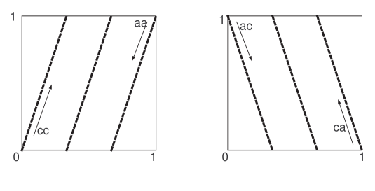
Figure 2: Weight points of $cc,aa$ and $ac,ca$ rings in weight space. x- and y-axis represent $2\Delta_{1}(j)$ and $2\Delta_{2}(j)$. Arrows represent the direction and starting point of corresponding ring as $j$ increases from 1 to n-1. Plot is drawn for $k_{1}=1,\;k_{2}=3$.

In order to compare these spectrum with $a_{1}$ and/or $a_{2}$ negative cases, we work out the weight of the states in Table 8.

$G$	$c$-ring	$2\Delta$	$a$-ring	$2\Delta$
$G_{cc}$	$u_{1}^{na_{1}}u_{2}^{na_{2}}$	$a_{1}+a_{2}$	${\bar{u}_{1}}^{n(1-a_{1})}{\bar{u}_{2}}^{n(1-a_{2})}$	$2-a_{1}-a_{2}$
$G_{ca}$	$u_{1}^{na_{1}}{\bar{u}}_{2}^{n(1-a_{2})}$	$a_{1}-a_{2}+1$	${\bar{u}_{1}}^{n(1-a_{1})}{u_{2}}^{na_{2}}$	$1-a_{1}+a_{2}$
$G_{ac}$	${\bar{u}}_{1}^{n(1-a_{1})}u_{2}^{na_{2}}$	$1-a_{1}+a_{2}$	${u_{1}}^{na_{1}}{\bar{u}_{2}}^{n(1-a_{2})}$	$a_{1}-a_{2}+1$
$G_{aa}$	${\bar{u}}_{1}^{n(1-a_{1})}{\bar{u}}_{2}^{n(1-a_{2})}$	$2-a_{1}-a_{2}$	${u_{1}}^{na_{1}}{u_{2}}^{na_{2}}$	$a_{1}+a_{2}$

Table 8: Monomial basis of chiral and anti-chiral rings and their weights for various choices of target space complex structures.

By comparing the two Table 3 and Table 8, it is clear that the spectrum of $ca$-ring of $n(k_{1},k_{2})$ theory is equal to the $cc$-chiral ring of $n(k_{1},-k_{2})$ theory. So the change in complex structure $u_{i}\to{\bar{u}_{i}}$ is equivalent to the change in generator $k_{i}\to-k_{i}$ keeping the complex structure fixed. For string theory, we have to consider all four different complex structures. That is, we may consider 4 sets of spectra generated by $(k_{1},k_{2})$, $(-k_{1},k_{2})$, $(k_{1},-k_{2})$ and $(-k_{1},-k_{2})$ all together.

Summarizing, we have shown that any of the lowest tachyon spectrum generated by the worldsheet fermions, can be considered as chiral state by choosing a worldsheet SUSY generator appropriately; any of them belongs to one of 4 classes: $cc$-, $ca$-, $ac$-, $aa$- ring depending on the choice of complex structure of ${\mathbb{C}}^{2}$. This is explicit in the Table 9.

($a_{1}-{1\over 2},a_{2}-{1\over 2}$)	$cc$	$ca$	$ac$	$aa$
$--$	$|0>$	$\psi_{2}|0>$	$\psi_{1}|0>$	$\psi_{1}\psi_{2}|0>$
$-+$	$\psi_{2}^{*}|0>$	$|0>$	$\psi_{1}\psi_{2}^{*}|0>$	$\psi_{1}|0>$
$+-$	$\psi_{1}^{*}|0>$	$\psi_{1}^{*}\psi_{2}|0>$	$|0>$	$\psi_{2}|0>$
$++$	$\psi_{1}^{*}\psi_{2}^{*}|0>$	$\psi_{1}^{*}|0>$	$\psi_{2}^{*}|0>$	$|0>$

Table 9: For a given twisted sector, any tachyon generated by worldsheet fermions is an element of one of the 4 possible chiral rings.

We emphasize that these chiral rings do not co-exist at the same time. For example, when $cc$-ring is active ( chosen), then $aa$-ring exists as its anti-chiral ring and other two are not chiral or anti-chiral ring. But for our purpose, for any tachyon state, there is a choice of complex structure in which the given state is a chiral primary. For example, if a tachyon in $ca$ ring is condensed, the spectrum of entire $ca$-ring is well controlled by the worldsheet supersymmetries generated by $G_{1}^{+},G_{2}^{-}$. As a consequence, we will be able to calculate the fate of those controlled spectrum. This is powerful since if we know that initial and final thoeries are described by an orbifold theories [1, 2, 3], knowing those of a few spectrum completely fixes entire tower of the string spectrum in the final theory. The same phenomena arise for all ${\mathbb{C}}^{r}/{\mathbb{Z}}_{n}$. Any worldsheet fermion generated tachyon state is a chiral primary by properly choosing the target space complex structure among $2^{r}$ possibilities defined by the $\sum_{i=1}^{r}G_{i}^{\pm}$. There are $2^{r}$ $(2,2)$ world sheet supersymmetries instead of one. In fact this happens for any tensor product of ${\cal N}=2$ SCFT’s.

We end this subsection with a few comments.

• The weight space is a lattice in torus of size $n\times n$. The identification of weights by modulo $n$ corresponds to shifting string modes. However, periodicity of the generator $(k_{1},k_{2})$ is $2n$ and $(k_{1},k_{2})$ and $(k_{1},k_{2}+n)$ do not generate the same theory in general. We choose the standard range of $k_{i}$ between $-n+1$ to $n-1$. This is because the GSO projection depends not only on the R-charge vector $(\{jk_{1}/n\},\{jk_{2}/n\})$ but also on the $G$-parity number $G=[jk_{1}/n]+[jk_{2}/n]$. We will come back to this when we discuss the GSO projection.

• When $n$ and $k_{i}$ are not relatively prime, we have a chiral primary whose R-charge vector is $(p/n,0)$. We call this as the reducible case and eliminate from our interests. This is a spectrum that is not completely localized at the tip of the orbifold. Sometimes, even in the case we started from non-reducible theory, a tachyon condensation leads us to the reducible case.

References

- [1] A. Adams, J. Polchinski and E. Silverstein, “Don’t panic! Closed string tachyons in ALE space-times,” JHEP 0110, 029 (2001) [arXiv:hep-th/0108075].
- [2] C. Vafa, “Mirror symmetry and closed string tachyon condensation,” arXiv:hep-th/0111051.
- [3] J. A. Harvey, D. Kutasov, E. J. Martinec and G. Moore, “Localized tachyons and RG flows,” arXiv:hep-th/0111154.
- [4] T. Takayanagi and T. Uesugi, “Orbifolds as Melvin geometry,” arXiv:hep-th/0110099.
- [5] Sang-Jin Sin, “Tachyon mass, c-function and Counting localized degrees of freedom,” Nucl. Phys. B637 (2002)395, arXiv:hep-th/0202097.
- [6] L. J. Dixon, D. Friedan, E. J. Martinec and S. H. Shenker, “The Conformal Field Theory Of Orbifolds,” Nucl. Phys. B 282, 13 (1987).
- [7] A. Dabholkar and C. Vafa, “tt* geometry and closed string tachyon potential,” arXiv:hep-th/0111155.
- [8] Sang-Jin Sin, “Localized tachyon mass and a g-theorem analogue,” arXiv:hep-th/xxyyddd.
- [9] D. A. Lowe and A. Strominger, “Strings near a Rindler or black hole horizon,” Phys. Rev. D 51, 1793(1995) [arXiv:hep-th/9410215].
-
[10]
E. J. Martinec and G. Moore,
“On decay of K-theory,”
arXiv:hep-th/0212059;
E. J. Martinec, “Defects, decay, and dissipated states,” arXiv:hep-th/0210231. - [11] A. Dabholkar, “Strings on a cone and black hole entropy,” Nucl. Phys. B 439, 650 (1995) [arXiv:hep-th/9408098].
- [12] J. R. Russo and A. A. Tseytlin, “Supersymmetric flux brane interssections and closed string tachyons”, JHEP 0111,065 (2001) [arXiv:hep-th/0110107].
- [13] C. Vafa, “Quantum Symmetries Of String Vacua,” Mod. Phys. Lett. A 4, 1615 (1989).