hep-th/0308008

We study IR/UV mixing effects in noncommutative supersymmetric Yang-Mills theories with gauge group $U(N)$ using background field perturbation theory. We compute three- and four-point functions of background fields, and show that the IR/UV mixed contributions to these correlators can be reproduced from an explicitly gauge-invariant effective action, which is expressed in terms of open Wilson lines.

$\sharp$ Present address: Department of Physics, Queen Mary College, London E1 4NS

1 Introduction

Quantum field theories on noncommutative spaces have attracted a lot of attention in the last few years. Part of this interest is motivated by the fact that noncommutative gauge theories appear as the low-energy limit of open strings in the presence of a constant $B$ field [1, 2, 3, 4]. Noncommutative theories are also very interesting from the purely field theoretical perspective, as they manifest novel features compared to their commutative cousins. The most interesting one is probably infrared/ultraviolet (IR/UV) mixing [5, 6]. Contrary to naive expectations based on commutative intuition, the high-energy degrees of freedom of noncommutative theories in general affect the physics at low-energy. In perturbation theory, the loop integrals in the planar sector of the noncommutative theory are exactly the same as in the commutative counterpart, which implies the same structure of divergences and same counterterms of the commutative theory. However, nonplanar diagrams are multiplied by phase factors of the form $e^{ik\cdot\theta\cdot p}$, where $k$ are external momenta and $p$ are loop momenta. This phase factor improves the UV-convergence of nonplanar diagrams, and typically renders them finite. But in the IR limit of the external momenta, $e^{\,ik\cdot\theta\cdot p}\rightarrow 1$ as $k\rightarrow 0$, the nonplanar diagrams become divergent and this is now an IR-divergence. This dramatically invalidates the naive expectations about a universal behaviour in the infrared for commutative and noncommutative theories, and the infrared regime of a noncommutative theory is in general different from that of its commutative counterpart [5, 6].

To explore this point further, in [9, 10] the low-energy wilsonian effective action for a large class of supersymmetric and non-supersymmetric theories was computed. The result was that, in the low-energy effective action, the $U(1)$ degrees of freedom decouple from the $SU(N)$ part, with IR/UV mixing affecting only the $U(1)$ part of the gauge group [10]. The leading order terms in the derivative expansion of the wilsonian effective action read [9, 10]:

$${S}_{\rm eff}\ \ni\ {1\over 4g^{2}_{\scriptscriptstyle 1}(k)}\ \int\!d^{4}x\,F^{\scriptscriptstyle U(1)}_{\mu\nu}F^{\scriptscriptstyle U(1)}_{\mu\nu}\ +\ {1\over 4g^{2}_{\scriptscriptstyle N}(k)}\ \int\!d^{4}x\,F^{\scriptscriptstyle SU(N)}_{\mu\nu}F^{\scriptscriptstyle SU(N)}_{\mu\nu}\ ,$$ (1.1)

where the coefficients in front of the gauge kinetic terms in (1.1) define the wilsonian coupling constants of the corresponding gauge factors. The running of the $U(1)$ has the following asymptotic behaviour [9, 10]:

$${1\over g^{2}_{\scriptscriptstyle 1}(k)}\,\rightarrow\,\pm{\alpha_{0}\over(4\pi)^{2}}\log k^{2}\ ,$$ (1.2)

where the plus (minus) sign corresponds to $k^{2}\to\infty$ ($k^{2}\to 0$), whereas for the $SU(N)$ gauge factor we have, in both limits, the usual (UV asymptotically free) running:

$${1\over g^{2}_{\scriptscriptstyle N}(k)}\,\rightarrow\,{\beta_{0}\over(4\pi)^{2}}\log k^{2}\ .$$ (1.3)

In the previous expressions (1.2), (1.3), $\beta_{0}$ is the first coefficient of the microscopic $\beta$-function, and $\alpha_{0}$ is a positive constant whose numerical value is determined by the field content of the theory, e.g. $\alpha_{0}=\beta_{0}\equiv 3N$ for pure $U(N)$ ${\cal N}=1$ super Yang-Mills (for more general situations see (5.5) and [9, 10, 11]). The change in the running of the $U(1)$ coupling in (1.2) is the manifestation of the IR/UV mixing, and occurs at a scale $k^{2}\sim M_{\scriptscriptstyle\rm NC}^{2}$, where $M_{\scriptscriptstyle\rm NC}\sim\theta^{-1/2}$ is the noncommutative mass.

In any non-supersymmetric theory, quadratic divergences appear in the gauge field polarisation tensor which would change the photon dispersion relation [6], and hence threaten the renormalizability of the theory. Interestingly, these quadratic divergences cancel in any supersymmetric theory, and in these theories we are left with the logarithmic infrared divergences in the effective $U(1)$ coupling encoded in (1.2) [6, 9]. Hence, supersymmetry appears to be a necessary ingredient for a noncommutative theory to be consistent [5, 6, 9]. For this reason, from now on we will fix our attention on supersymmetric theories.

The peculiar behaviour discussed above for the $U(1)$ effective coupling constant was interpreted in [11] as having a full noncommutative $U(N)$ gauge theory in the ultraviolet, which in the low-energy limit appears as a commutative $SU(N)$ theory, with the $U(1)$ degrees of freedom which become progressively more weakly coupled (i.e. unobservable) in the infrared. In the same paper, a mechanism for supersymmetry breaking was suggested where the $U(1)$ degrees of freedom act as the hidden sector, breaking supersymmetry at a scale potentially much lower than the noncommutativity scale, and eventually becoming unobservable in the infrared due to the IR/UV mixing. This IR/UV mixing therefore acquires the status of a very welcome feature of noncommutative theory, rather than being a field-theoretical illness of it.

The expression (1.1) for the effective action would suggest that the noncommutative $U(N)$ gauge symmetry is broken at low energy; despite appearances, this is not the case. In [12] it was argued that the full one-loop effective action for the ${\cal N}=4$ theory is gauge invariant (see also [14, 15, 13]); nonplanar diagrams give gauge-noninvariant contributions to e.g. the four-point function, but in the Ward identities these terms are precisely cancelled by gauge-noninvariant terms in the five-point function [12]. This mechanism of cancellations between different $n$-point functions is quite a clear clue for the presence of Wilson lines in the expression for the effective action. Indeed, in [17, 16], a gauge-invariant completion of (1.1) was proposed which involves open Wilson lines [18, 19, 20]. It was conjectured in [17] that the the IR/UV mixed contribution to the effective action of a supersymmetric gauge theory can be reproduced by the following $U(N)$ gauge-invariant term:

$$S^{(1)}_{\rm eff}\,=\,-\frac{{\cal C}}{4}\,\int\!\!\frac{d^{4}p}{(2\pi)^{4}}\,{\cal O}^{\mu\nu}(-p)\,T(p)\,{\cal O}_{\mu\nu}(p)\ ,$$ (1.4)

where the gauge-invariant operator ${\cal O}_{\mu\nu}$ is defined by

$${\cal O}_{\mu\nu}(p)={\rm Tr}\int\!d^{4}x\ L_{\star}\left(F_{\mu\nu}(x)\,e^{\,\int_{0}^{1}\!\!d\sigma\,{\tilde{p}}^{\mu}A_{\mu}(x+{\tilde{p}}\,\sigma)}\right)\star e^{ipx}\ ,$$ (1.5)

and $L_{\star}$ stands for integration along the open Wilson line together with path ordering with respect to the star-product [21]. The matching of (1.4) with the analytic results [9] for the $U(1)$ effective coupling constant $1/g^{2}_{1}(k)$ of (1.2) determines the function $T(p)$ and the numerical constant ${\cal C}$ appearing in (1.4). One easily finds that

$$T(p)=\frac{2}{(4\pi)^{2}}\int_{0}^{1}\!\!dx\,K_{0}(\sqrt{x(1-x)}\,|p||\tilde{p}|)\ ,$$ (1.6)

where $K_{0}$ is a Bessel function, with $K_{0}(z)\to-\log(z/2)$ as $z\to 0$. Moreover, ${\cal C}=2\alpha_{0}/N$, where $\alpha_{0}$ is defined in (1.2).

In this paper we would like confirm the interesting conjecture of [17] with an explicit field theory calculation. To start probing the presence of the Wilson line operator in (1.5) we need to calculate an $n$-point function of gauge fields with $n\geq 3$; for this reason, we will concentrate on the cases of three- and four-point functions of background fields. Our formalism is, however, general, and allows in principle to calculate generic $n$-point correlators. We will focus our attention on a generic ${\cal N}=1$ supersymmetric field theory with $N_{\rm f}$ adjoint chiral multiplets and make use of the background field method. The case $N_{\rm f}=0$ corresponds to pure ${\cal N}=1$ super Yang-Mills, whereas for $N_{\rm f}=1,3$ we have the ${\cal N}=2$ and ${\cal N}=4$ theories, respectively. The results of our computations confirm the presence of the term (1.4) in the effective action. However, our results also show that we need to include another term $S^{(2)}_{\rm eff}$ in the effective action, which can be written as

$$S^{(2)}_{\rm eff}=\frac{{{\cal C}}}{2}\int\!\!\frac{d^{4}p}{(2\pi)^{4}}\,{\cal O}_{F^{2}}(p)\ W^{\prime}(-p)\,T(p)\ ,$$ (1.7)

where

$${\cal O}_{F^{2}}(p)={{\rm Tr}}\int\!d^{4}x\ L_{\star}\left(F_{\mu\nu}(x)F^{\mu\nu}(x)e^{\,\int_{0}^{1}\!\!d\sigma\,\tilde{p}^{\mu}A_{\mu}(x+\tilde{p}\sigma)}\star e^{ipx}\right)\,\ ,$$ (1.8)

and ${\cal W^{\prime}}(p)$ denotes the open Wilson line operator ${\cal W}(p)$ with the ${\cal O}(A^{0})$ term subtracted, where, in our conventions

$${\cal W}(p)={\rm Tr}\int\!d^{4}x\ P_{\star}\left(e^{\,\int_{0}^{1}\!\!d\sigma\,{\tilde{p}}^{\mu}A_{\mu}(x+{\tilde{p}}\,\sigma)}\right)\star e^{ipx}\ .$$ (1.9)

$S^{(2)}_{\rm eff}$ is manifestly gauge invariant, and again contains open Wilson lines.

The appearance of the term $S^{(2)}_{\rm eff}$ in (1.7) is not unexpected. Indeed, similar contributions were predicted in [23], where a wilsonian calculation of the effective action was performed using the matrix model approach to noncommutative gauge theories. Similar results were also obtained in [24] using the bosonic world-line approach. In the first version of this paper we proposed to use the following expression, instead than (1.7):

$${\tilde{S}}^{(2)}_{\rm eff}=-i\,\frac{{\cal C}}{4}\int\!\!\frac{d^{4}q_{1}}{(2\pi)^{4}}\frac{d^{4}q_{2}}{(2\pi)^{4}}\,{\cal Q}(-q_{1},-q_{2})\ \theta^{\mu\nu}{\cal O}_{\mu\nu}(q_{1}+q_{2})\,T(q_{1}+q_{2})\ ,$$ (1.10)

where

$${\cal Q}(p,q)={{\rm Tr}}\int\!d^{4}x\ L_{\star}\left(F_{\mu\nu}(x)F^{\mu\nu}(x)e^{\,\int_{0}^{1}\!\!d\sigma\,\tilde{p}^{\mu}A_{\mu}(x+\tilde{p}\sigma)}\star e^{ipx}\right)\,{\sin(q\tilde{p}/2)\over q\tilde{p}}\ .$$ (1.11)

The interaction term in (1.10), though manifestly gauge invariant, is not satisfactory as it stands, since $\theta^{\mu\nu}$ appears in (1.10) not only inside the Wilson lines but also explicitly. This, in turns, would render its interpretation from the D-brane perspective very difficult. It is easy to check that, once we expand the Wilson line in (1.7) up to ${\cal O}({A})$, this term contributes to the three-point function in the same way as the term in (1.10) does. Indeed, we will show that (1.7) and (1.10) both produce a contribution to the three-point function which is in precise agreement with the direct calculation in the microscopic theory. Of course, at the level of four-point functions (1.7) and (1.10) start producing contributions which are different. By comparing the perturbative result for a four-point function to the corresponding result derived from the effective action, we will be able in the next sections to confirm that (1.7) is the correct expression to be incorporated in the effective action (rather than (1.10)), as also suggested by D-brane physics [23].

Let us mention that it would be very nice to have complete control on generic $n$-point functions (or at least on the IR/UV mixed contributions), and use this knowledge to derive the full low–energy effective action. An interesting and simple way to evaluate the IR/UV mixed quadratically divergent contributions (the poles) of generic $n$-point functions in a $U(1)$ non-supersymmetric gauge theory was devised in section (3.1) of [17]. Unfortunately, simplifications similar to those exploited in [17] seem to be lacking in the case at hand. It would be interesting to apply the bosonic worldline approach, used in [24] for non-supersymmetric theories, to the case of supersymmetric theories considered here, and see if that formalism would lead to more tractable expressions than those obtained using conventional background perturbation theory.

The plan of the rest of this paper is as follows. In section 2 we will obtain the contributions to the three- and four-point functions of gauge fields from the terms $S^{(1)}_{\rm eff}$ and $S^{(2)}_{\rm eff}$ in the effective action, Eqs. (1.4) and (1.7), respectively. Sections 3 contains the set-up for the application of the background field method to noncommutative gauge theories, and our Feynman rules. Using the background field method, we calculate in section 4 the three- and four-point functions of background fields. In section 5 we compare the perturbative results derived in section 4 to the result obtained in section 2 from the effective action, finding agreement. For other related work on noncommutative theories, see [7, 8, 27, 28, 29, 30, 31, 32, 33, 34, 35, 36, 37, 38, 39, 40, 41, 42, 44, 43] and references therein.

Before concluding this introduction, we would like to mention that IR/UV mixing also appears [25] in the recently discussed field theories on non(anti)commuting superspace [26]. Again, the resummed effective action appears to contain open Wilson lines in superspace [25].

2 Three- and four-point functions from an effective action with Wilson lines

2.1 The three-point function

We begin by calculating the contribution from the effective interaction in (1.4) to the three-point function

$$\Gamma_{\mu\nu\rho}^{ABC}(k_{1},k_{2},k_{3})\,:=\,\int\!\!\prod_{i=1}^{3}\,\frac{d^{4}x_{i}}{(2\pi)^{4}}\ e^{\,i\sum_{i=1}^{3}k_{i}x_{i}}\,\langle\,A_{\mu}^{A}(x_{1})\,A_{\nu}^{B}(x_{2})\,A_{\rho}^{C}(x_{3})\,\rangle\ .$$ (2.1)

In order to calculate the contribution from (1.4) we need only to expand the expression for ${\cal O}_{\mu\nu}(p)$ in (1.5) up to order $A^{2}$. We then Fourier transform and use (A.6) and (A.3), to get:

$${\cal O}_{\mu\nu}(p)=l_{\mu\nu}(p)+q^{(1)}_{\mu\nu}(p)+q^{(2)}_{\mu\nu}(p)+{\cal O}(A^{3})\ ,$$ (2.2)

where

$$l_{\mu\nu}(p) = -\sqrt{N\over 2}\ \left[p_{\mu}A_{\nu}^{0}(p)-p_{\nu}A_{\mu}^{0}(p)\right]\ ,$$ (2.3)

$$q^{(1)}_{\mu\nu}(p) = iA_{\mu}^{A}(q)A_{\nu}^{A}(p-q)\ \sin\frac{q\tilde{p}}{2}\ ,$$

$$q^{(2)}_{\mu\nu}(p) = i\int\!\!\frac{d^{4}q}{(2\pi)^{4}}\,\left[q_{\mu}A_{\nu}^{A}(q)-q_{\nu}A_{\mu}^{A}(q)\right](\tilde{p}\cdot A^{A}(p-q))\ {\sin(q\tilde{p}/2)\over q\tilde{p}}\ .$$

Using (2.2), we get the following contribution to the three-point function from the effective action $S^{(1)}_{\rm eff}$ of (1.4):

$$\left.\Gamma^{ABC}_{\mu\nu\rho}(k_{1},k_{2},k_{3})\right|_{S^{(1)}_{\rm eff}} = i{\cal C}\sqrt{\frac{N}{2}}\,{\sin(k_{2}\tilde{k}_{3}/2)\over k_{2}\tilde{k}_{3}}\ (2\pi)^{4}\,\delta^{(4)}(k_{1}+k_{2}+k_{3})$$

$$\cdot\,\Bigl{\{}T(k_{1})\ \delta^{A0}\delta^{BC}\left[\tilde{k}_{1{\nu}}P^{13}_{\rho\mu}+\tilde{k}_{1{\rho}}P^{12}_{\nu\mu}+(k_{2}\tilde{k}_{3})\,Q^{1}_{\mu,\nu\rho}\right]$$

$$\ +T(k_{2})\ \delta^{B0}\delta^{CA}\left[\tilde{k}_{2{\mu}}P^{23}_{\rho\nu}+\tilde{k}_{2{\rho}}P^{12}_{\nu\mu}+(k_{2}\tilde{k}_{3})\,Q^{2}_{\nu,\rho\mu}\right]$$

$$\ +T(k_{3})\ \delta^{C0}\delta^{AB}\left[\tilde{k}_{3{\mu}}P^{23}_{\rho\nu}+\tilde{k}_{3{\nu}}P^{13}_{\rho\mu}+(k_{2}\tilde{k}_{3})\,Q^{3}_{\rho,\mu\nu}\right]\Bigr{\}}\ ,$$

where we have defined

$$P^{ij}_{\mu\nu}\ :=\ \delta_{\mu\nu}(k^{i}\cdot k^{j})\,-\,k^{i}_{\mu}k^{j}_{\nu}\ ,\qquad Q^{i}_{\rho,\mu\nu}\ :=\ \delta_{\rho\mu}\,k^{i}_{\nu}\,-\,\delta_{\rho\nu}\,k^{i}_{\mu}\ .$$ (2.6)

In a similar way we can calculate the contribution to the three-point function from the term $S^{(2)}_{\rm eff}$ in (1.7), obtaining:

$$\left.\Gamma^{ABC}_{\mu\nu\rho}(k_{1},k_{2},k_{3})\right|_{S^{(2)}_{\rm eff}}=i{\cal C}\sqrt{\frac{N}{2}}\ {\sin(k_{2}\tilde{k}_{3}/2)\over k_{2}\tilde{k}_{3}}\ (2\pi)^{4}\,\delta^{(4)}(k_{1}+k_{2}+k_{3})$$ (2.7)

$$\qquad\qquad\cdot\,\left\{\delta^{A0}\delta^{BC}\,T(k_{1})\,\tilde{k}_{1\mu}P_{\rho\nu}^{23}\,+\,\delta^{B0}\delta^{AC}\,T(k_{2})\,\tilde{k}_{2\nu}P_{\mu\rho}^{31}\,+\,\delta^{C0}\delta^{AB}\,T(k_{3})\,\tilde{k}_{3\rho}P_{\nu\mu}^{12}\right\}\ .$$

2.2 The four-point function

In this section we compute the contributions to the four-point function obtained from the effective action $S^{(1)}_{\rm eff}$ and $S^{(2)}_{\rm eff}$ given in (1.4), (1.7), respectively. For the sake of simplicity we will restrict ourselves to the case of noncommutative $U(1)$ gauge group, and compute the four-point function

$$\Gamma_{\mu\nu\rho\sigma}(k_{1},k_{2},k_{3},k_{4})\,:=\,\int\!\!\prod_{i=1}^{4}\,\frac{d^{4}x_{i}}{(2\pi)^{4}}\ e^{\,i\sum_{i=1}^{4}k_{i}x_{i}}\,\langle\,A_{\mu}(x_{1})\,A_{\nu}(x_{2})\,A_{\rho}(x_{3})\,A_{\sigma}(x_{4})\,\rangle\ .$$ (2.8)

The result for $\Gamma_{\mu\nu\rho\sigma}(k_{1},k_{2},k_{3},k_{4})$ is better expressed in terms of the quantities $J_{2}(k_{1},k_{2})$ and $J_{3}(k_{1},k_{2},k_{3})$ introduced in [21] (see Appendix B of that paper), where

$$J_{2}(k_{1},k_{2}) = {\sin{k_{1}\tilde{k}_{2}\over 2}\over{k_{1}\tilde{k}_{2}\over 2}}\ ,$$ (2.9)

$$J_{3}(k_{1},k_{2},k_{3}) = {\sin{k_{2}\tilde{k}_{3}\over 2}\,\sin{k_{1}(\tilde{k}_{2}+\tilde{k}_{3})\over 2}\over{(k_{1}+k_{2})\tilde{k}_{3}\over 2}\,{k_{1}(\tilde{k}_{2}+\tilde{k}_{3})\over 2}}\ +\ {{\sin{k_{1}\tilde{k}_{3}\over 2}\,\sin{k_{2}(\tilde{k}_{1}+\tilde{k}_{3})\over 2}}\over{{(k_{1}+k_{2})\tilde{k}_{3}\over 2}\,{k_{2}(\tilde{k}_{1}+\tilde{k}_{3})\over 2}}}\ .$$ (2.11)

Not surprisingly, the functions $J_{2}(k_{1},k_{2})$ and $J_{3}(k_{1},k_{2},k_{3})$ [21] arise in the context of noncommutative effective action for the one-loop $F^{4}$ term in ${\cal N}=4$ super Yang-Mills.

In the same way as it was done for the three-point function, one finds that the contribution to the four-point function generated by the term (1.4) is given by the following expression:

$$\left.\Gamma_{\mu\nu\rho\sigma}(k_{1},k_{2},k_{3},k_{4})\right|_{S^{(1)}_{\rm eff}}\,=\,\,\,\!\!\!\!(2\pi)^{4}\,\delta^{(4)}(k_{1}+\cdots+k_{4})\,\Bigl{\{}\,2\,T(k_{4})\,\cdot$$ (2.12)

$$\!\!\!\!\cdot\Bigl{[}\tilde{k}^{4}_{\rho}Q^{4}_{\sigma,\nu\mu}\sin{k_{1}\tilde{k}_{2}\over 2}J_{2}(k_{3},k_{4})+\tilde{k}^{4}_{\nu}Q^{4}_{\sigma,\rho\mu}\sin{k_{1}\tilde{k}_{3}\over 2}J_{2}(k_{2},k_{4})+\tilde{k}^{4}_{\mu}Q^{4}_{\sigma,\rho\nu}\sin{k_{2}\tilde{k}_{3}\over 2}J_{2}(k_{1},k_{4})\Bigr{]}$$ (2.13)

$$-T(k_{4})\,J_{3}(k_{1},k_{2},k_{3})\,\Bigl{[}P^{41}_{\mu\sigma}\,\tilde{k}_{\nu}^{4}\,\tilde{k}_{\rho}^{4}\,+\,P^{42}_{\nu\sigma}\,\tilde{k}_{\mu}^{4}\,\tilde{k}_{\rho}^{4}\,+\,P^{43}_{\rho\sigma}\,\tilde{k}_{\mu}^{4}\,\tilde{k}_{\nu}^{4}\Bigr{]}$$ (2.14)

$$-T(k_{1}+k_{2})\Bigl{[}\delta_{\mu\rho}\delta_{\nu\sigma}\sin{k_{1}\tilde{k}_{2}\over 2}\sin{k_{3}\tilde{k}_{4}\over 2}+\,{1\over 2}P^{13}_{\rho\mu}(\tilde{k}_{1}+\tilde{k}_{2})_{\nu}(\tilde{k}_{3}+\tilde{k}_{4})_{\sigma}\,J_{2}(k_{1},k_{2})J_{2}(k_{3},k_{4})$$ (2.15)

$$+\,{1\over 2}Q^{3}_{\mu,\nu\rho}\sin{k_{1}\tilde{k}_{2}\over 2}(\tilde{k}_{3}+\tilde{k}_{4})_{\sigma}\,J_{2}(k_{3},k_{4})\,+\,{1\over 2}\,Q^{1}_{\rho,\sigma\mu}\sin{k_{3}\tilde{k}_{4}\over 2}(\tilde{k}_{1}+\tilde{k}_{2})_{\nu}\,J_{2}(k_{1},k_{2})\Bigr{]}$$ (2.16)

$$\ \ +\ \ {\rm permutations}\,\Bigr{\}}\ .$$ (2.17)

Notice the appearance of the function $J_{3}(k_{1},k_{2},k_{3})$ in the previous expression (2.12).

We now compute the contribution to the four-point function derived from the term (1.7). After some straightforward calculations, one gets:

$$\left.\Gamma_{\mu\nu\rho\sigma}(k_{1},k_{2},k_{3},k_{4})\right|_{S^{(2)}_{\rm eff}}\,=\,\,\,\!\!\!\!(2\pi)^{4}\,\delta^{(4)}(k_{1}+\cdots+k_{4})\,\Bigl{\{}\,2T(k_{4})\,\tilde{k}^{4}_{\sigma}\cdot$$ (2.18)

$$\!\!\!\!\cdot\Bigl{[}-Q^{1}_{\mu,\rho\nu}{k_{2}\tilde{k}_{3}\over 2}J_{2}(k_{2},k_{3})\cos{k_{1}\tilde{k}_{4}\over 2}-Q^{2}_{\nu,\rho\mu}{k_{1}\tilde{k}_{3}\over 2}J_{2}(k_{1},k_{3})\cos{k_{2}\tilde{k}_{4}\over 2}-Q^{3}_{\rho,\mu\nu}{k_{2}\tilde{k}_{1}\over 2}J_{2}(k_{1},k_{2})\cos{k_{3}\tilde{k}_{4}\over 2}\Bigr{]}$$ (2.19)

$$+{1\over 2}\,P^{12}_{\nu\mu}\,\tilde{k}^{4}_{\rho}\,J_{2}(k_{3},k_{4})\,\cos{k_{1}\tilde{k}_{2}\over 2}\,+\,{1\over 2}\,P^{13}_{\rho\mu}\,\tilde{k}^{4}_{\nu}\,J_{2}(k_{2},k_{4})\,\cos{k_{1}\tilde{k}_{3}\over 2}\,+\,{1\over 2}\,P^{23}_{\rho\nu}\,\tilde{k}^{4}_{\mu}\,J_{2}(k_{1},k_{4})\,\cos{k_{2}\tilde{k}_{3}\over 2}\Bigr{]}$$ (2.20)

$$-{1\over 2}\,\Bigl{[}T(k_{1}+k_{2})J_{2}(k_{1},k_{2})\cos{k_{3}\tilde{k_{4}}\over 2}(\tilde{k}_{1}+\tilde{k}_{2})_{\mu}(\tilde{k}_{1}+\tilde{k}_{2})_{\nu}P^{34}_{\sigma\rho}+$$ (2.21)

$$\qquad\!T(k_{1}+k_{3})J_{2}(k_{1},k_{3})\cos{k_{2}\tilde{k_{4}}\over 2}(\tilde{k}_{1}+\tilde{k}_{3})_{\mu}(\tilde{k}_{1}+\tilde{k}_{3})_{\rho}P^{24}_{\sigma\nu}+$$ (2.22)

$$\,\,\qquad\!T(k_{1}+k_{4})J_{2}(k_{1},k_{4})\cos{k_{1}\tilde{k_{4}}\over 2}(\tilde{k}_{1}+\tilde{k}_{4})_{\mu}(\tilde{k}_{1}+\tilde{k}_{4})_{\sigma}P^{32}_{\nu\rho}\Bigr{]}\ +\ {\rm permutations}\ \Bigl{\}}\ .$$ (2.23)

3 A lightning review of the background field method

We will now apply the background field method to the study of correlators in a generic noncommutative theory with gauge group $U(N)$. Our analysis follows closely the approach of [9], to which we refer the reader for details of the application of the background field method to noncommutative theories.

We will decompose the gauge field $A_{\mu}$ as $A_{\mu}=B_{\mu}+Q_{\mu}$, where $B_{\mu}$ is a slowly varying background field, and $Q_{\mu}$ represents the high-energy fluctuations. After functionally integrating over the high-frequency fields, we are left with an effective action for the background fields $B_{\mu}$. Importantly, this effective action is invariant with respect to gauge transformations of the background field, $B\to\Omega(B+\partial)\Omega^{\dagger}$, where $\Omega$ is an element of the noncommutative $U(N)$, $\Omega:=e_{\star}^{\alpha_{A}T^{A}}$.

The action functional which describes the dynamics of a spin-$j$ noncommutative field $\phi_{m,a}$ in the representation r of the gauge group in the background of $B_{\mu}$ has the general form [9, 45]

$$S[\phi] = -\int\!d^{4}x\ \phi_{m,a}\star\left(-D^{2}(B)\delta_{mn}\delta^{ab}+2i(F_{\mu\nu}^{B})^{ab}{\textstyle{1\over 2}}J^{\mu\nu}_{mn}\right)\star\phi_{n,b}$$ (3.1)

$$\equiv -\int\!d^{4}x\ \phi_{m,a}\star[\Delta_{j,{\bf r}}]_{mn}^{ab}\star\phi_{n,b}\ \ .$$ (3.2)

Here $a,b$ are indices of the representation r of noncommutative $U(N)$, $F^{ab}\equiv\sum_{A=1}^{N^{2}}F^{A}t^{A}_{ab}$, and $m,n$ are spin indices and $J^{\mu\nu}_{mn}$ are the generators of the euclidean Lorentz group appropriate for the spin of the field $\phi$, i.e. $J\,=\,0$ for spin $0$ fields, $J^{\mu\nu}_{\rho\sigma}\,=\,i\,(\delta^{\mu}_{\rho}\,\delta^{\nu}_{\sigma}\,-\,\delta^{\nu}_{\rho}\,\delta^{\mu}_{\sigma})$ for vectors, and $[J^{\mu\nu}]_{\alpha}^{\ \beta}\,=\,{\textstyle{i\over 2}}\,[\sigma^{\mu\nu}]_{\alpha}^{\ \beta}$ for Weyl fermions.

We consider a generic supersymmetric theory with adjoint chiral multiplets, therefore we only need to know the action of $\Delta_{j,{\bf r}}$ on adjoint fields. In this case, it easy to see from (3.1) that $\Delta_{j,{\bf\scriptscriptstyle G}}\star\phi$ gives

$$\Delta_{j,{\bf\scriptscriptstyle G}}\star\phi=-\partial^{2}\phi-\left[(\partial_{\mu}B_{\mu}),\phi\right]_{\star}-2\left[B_{\mu}\partial_{\mu},\phi\right]_{\star}-\left[B_{\mu},\left[B_{\mu},\phi\right]_{\star}\right]_{\star}+2i\left(\frac{1}{2}J^{\mu\nu}\left[F_{\mu\nu}^{B},\phi\right]_{\star}\right)\ .$$ (3.3)

The one-loop expression for the effective action reads [9]

$$S_{\rm eff}[B]=-\frac{1}{2g^{2}}\int\!d^{4}x\ {\rm Tr}\,F_{\mu\nu}^{B}\star F_{\mu\nu}^{B}-\sum_{j,{\bf r}}\alpha_{j}\log\,{\rm det}_{\star}\Delta_{j,{\bf r}}\ .$$ (3.4)

The sum in (3.4) is extended to all fields in the theory, including ghosts and gauge fields. $\alpha_{j}$ is equal to $+1$ ($-1$) for ghost (scalar) fields and to $+1/2$ ($-1/2$) for Weyl fermions (gauge fields). Finally, the functional star-determinants are computed by

$$\log\,{\rm det}_{\star}\Delta_{j,{\bf r}} \equiv \log\,{\rm det}_{\star}\left[-\partial^{2}+{\cal K}(B)_{j,{\bf r}}\right]$$

$$= \log\,{\rm det}_{\star}(-\partial^{2})+{\rm tr}_{\star}\log\,\left[1+(-\partial^{2})^{-1}{\cal K}(B)_{j,{\bf r}}\right]\ .$$

The first term on the second line of (3) contributes only to the vacuum loops and will be dropped in the following. The second term on the last line of (3) has a full expansion in terms of Feynman diagrams, and on this term we concentrate our attention.

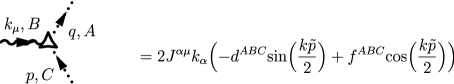
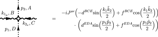
Figure 1: Feynman rules for $U(N)$. The wavy lines represent the background fields, the dotted lines the high-virtuality fields.

3.1 Feynman Rules

We follow the conventions of [10], whose Feynman rules we will use. We only need to compute one additional interaction vertex, which originates from the commutator term in the field strength $F_{\mu\nu}^{B}$ appearing in the last term of (3.3). Using (A.6) and (A.3) this term can be written as:

$$2i{\rm Tr}\int\!d^{4}x\;\overline{\phi}J^{\mu\nu}\star[[B_{\mu},B_{\nu}]_{\star},\phi]_{\star}\,=\,\int\!\!\frac{d^{4}p^{\prime}}{(2\pi)^{4}}\frac{d^{4}q_{1}}{(2\pi)^{4}}\frac{d^{4}q_{2}}{(2\pi)^{4}}\frac{d^{4}p}{(2\pi)^{4}}(2\pi)^{4}\delta^{(4)}\Bigl{(}p^{\prime}+q_{1}+q_{2}+p\Bigr{)}\\ \cdot\,\bar{\phi}^{A}(p^{\prime})B_{\mu}^{B}(q)B_{\nu}^{C}(q_{2})\phi^{D}(p)\Bigl{[}-iJ^{\mu\nu}\Bigl{(}-d^{BCE}\sin\Bigl{(}\frac{q_{1}\tilde{q}_{2}}{2}\Bigr{)}+f^{BCE}\cos\Bigl{(}\frac{q_{1}\tilde{q}_{2}}{2}\Bigr{)}\Bigr{)}\\ \cdot\,\Bigl{(}f^{EDA}\cos\Bigl{(}\frac{p\tilde{p}^{\prime}}{2}\Bigr{)}+d^{EDA}\sin\Bigl{(}\frac{p\tilde{p}^{\prime}}{2}\Bigr{)}\Bigr{)}\Bigr{]}\ .$$ (3.6)

The complete set of Feynman rules is shown in figure 1.

We denote by a triangle and a star the so-called “$J$-vertices”, second and fourth line in the Feynman rules of figure 1 respectively, which are specific to the background field method.

4 Perturbative calculations in the microscopic theory

We now move on to the background field method computation of Green’s functions in the microscopic theory. For convenience, we present the three-point function and four-point function calculations separately.

4.1 The three-point function of background fields

We start with the calculation of the three-point function of background gauge fields $\Gamma_{\mu\nu\rho}^{ABC}(k_{1},k_{2},k_{3})$ defined in (2.1).

Figure 2: Feynman diagrams with no $J$-vertices.

To this end, we will need to expand the logarithm in (3.4) up to three powers of the background field. The resulting Feynman diagrams are shown in figures 2-5 (where we do not draw permutations of the diagrams).

The Feynman diagrams can be conveniently classified according to the number of $J$-vertices they contain. Diagrams with no $J$-vertices, represented in figure 2, give a vanishing contribution to the correlator. This is because each of these diagrams gets a factor of ${\rm Tr}\,\mbox{1 \kern-5.89996pt{\rm l}}_{j}\equiv d(j)$ from the trace over spin indices, where $d(j)$ is the number of spin components of the field, $d(j)=1$ for scalars, $2$ for Weyl fermions and $4$ for gauge fields, respectively. We focus only on supersymmetric theories, where the cancellation between fermionic and bosonic degrees of freedom implies that

$$\sum_{j}\alpha_{j}\,d(j)=0\ .$$ (4.1)

Therefore, each diagram which no $J$-vertices vanishes separately when it is summed over all the fields in the theory.

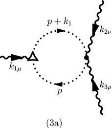
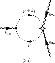
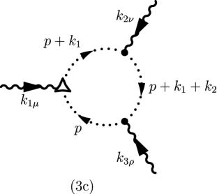
Figure 3: Feynman diagrams with a single insertion of $J$-vertices (denoted by a triangle and a star).

Similarly, diagrams with exactly one insertion of the $J$-vertices (figure 3) vanish, since the trace over spin indices gives ${\rm Tr}\,J^{\mu\nu}=0$.

With these simplifications, we are left with the diagrams of figures 4 and 5, which we now compute. We will calculate these diagrams in a low-energy approximation where the background fields have a much smaller momentum than the cut-off for the fluctuating fields, so that $k_{i}k_{j}\to 0$, while we keep $k_{i}\tilde{k}_{j}$ finite [14, 15, 12]. This low-energy approximation has the great advantage that all of the integrals over the loop momentum can be performed explicitly [13, 14] (see also the discussion after (4.1)).

We first consider diagrams with two $J$-vertices, represented in figure 4.

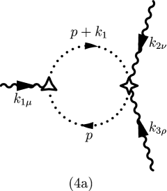
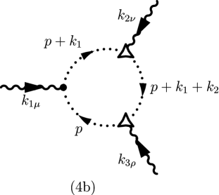
Figure 4: Feynman diagrams with two $J$-vertices.

The contribution to the correlator $\Gamma_{\mu\nu\rho}^{ABC}(k_{1},k_{2},k_{3})$ from diagram (4a) is:

$$-2i\Bigl{(}\sum_{j}\alpha_{j}\,{\rm Tr}\,(J^{\nu\rho}J^{\alpha\mu})_{j}\Bigr{)}\,\,(2\pi)^{4}\delta^{(4)}(k_{1}+k_{2}+k_{3})\int\!\!\frac{d^{4}p}{(2\pi)^{4}}\,k_{1{\alpha}}\frac{\delta^{DF}}{p^{2}}\frac{\delta^{EG}}{(p+k_{1})^{2}}$$

$$\Bigl{[}-d^{EAD}\sin\Bigl{(}\frac{k_{1}\tilde{p}}{2}\Bigr{)}+f^{EAD}\cos\Bigl{(}\frac{k_{1}\tilde{p}}{2}\Bigr{)}\Bigr{]}\Bigl{[}-d^{CBH}\sin\Bigl{(}\frac{k_{2}\tilde{k}_{3}}{2}\Bigr{)}+f^{CBH}\cos\Bigl{(}\frac{k_{2}\tilde{k}_{3}}{2}\Bigr{)}\Bigr{]}$$

$$\Bigl{[}d^{HGF}\sin\Bigl{(}\frac{(p+k_{1})\tilde{p}}{2}\Bigr{)}+f^{HGF}\cos\Bigl{(}\frac{(p+k_{1})\tilde{p}}{2}(p+k_{1})\tilde{p}\Bigr{)}\Bigr{]}\ ,$$ (4.2)

where the sum is over all the fields in the theory. We can simplify the products of $d$’s and $f$’s in (4.2) by using the relations derived in (2.8)–(2.11) of [32]. In addition, the product of $J$’s can be rewritten using

$${\rm Tr}(J^{\mu\rho}J^{\nu\lambda})_{j}\ =\ C(j)\,(\delta^{\mu\nu}\delta^{\rho\lambda}-\delta^{\mu\lambda}\delta^{\nu\rho})\ ,$$ (4.3)

where

$$C(j)\equiv\quad 0\quad{\rm for\,scalars,}\qquad\quad\frac{1}{2}\quad{\rm for\,Weyl\,\,fermions,}\qquad 2\quad{\rm for\,vectors}.$$ (4.4)

The remaining integrals can then be evaluated by first writing the sines and cosines in terms of exponentials, and then using

$$\int\!\!{\frac{d^{4}p}{(2\pi)^{4}}}\,{\frac{e^{ip\tilde{k}}}{p^{2}(p+k)^{2}}}={\frac{2}{(4\pi)^{2}}}\int_{0}^{1}\!\!dx\ K_{0}(\sqrt{A}|k||\tilde{k}|)\,\equiv\,T(k)\ \ ,$$ (4.5)

where $A=x(1-x)$ and the function $T$ is the same as in (1.6). In this way, the contribution to the three-point function from diagram (4a) (and its permutations) becomes:

$$[\Gamma_{\mu\nu\rho}^{ABC}(k_{1},k_{2},k_{3})]_{\rm 4a} = 4i\,\Bigl{(}\sum_{j}\alpha_{j}\,C(j)\Bigr{)}\,\sqrt{2N}\,(2\pi)^{4}\delta^{(4)}(k_{1}+k_{2}+k_{3})\,\sin\Bigl{(}\frac{k_{2}\tilde{k}_{3}}{2}\Bigr{)}$$ (4.7)

$$\!\!\!\!\!\Bigl{[}T(k_{1})\,Q^{1}_{\mu,\rho\nu}\,\delta^{A0}\delta^{BC}+T(k_{2})\,Q^{2}_{\nu,\mu\rho}\,\delta^{B0}\delta^{AC}+T(k_{3})\,Q^{3}_{\rho,\nu\mu}\delta^{C0}\delta^{AB}\,\Bigr{]}\ .$$

Diagram (4b) contributes to the correlator $\Gamma_{\mu\nu\rho}^{ABC}(k_{1},k_{2},k_{3})$ as:

$$4i\,\Bigl{(}\sum_{j}\alpha_{j}\,{\rm Tr}\,(J^{\alpha\nu}J^{\beta\rho})_{j}\Bigr{)}\,\,(2\pi)^{4}\delta^{(4)}(k_{1}+k_{2}+k_{3})\,$$ (4.8)

$$\int\!\!\frac{d^{4}p}{(2\pi)^{4}}\,k_{2\alpha}k_{3\beta}(2p+k_{1})_{\mu}\,\frac{\delta^{EF}}{p^{2}}\frac{\delta^{GH}}{(p+k_{1})^{2}}\frac{\delta^{IJ}}{(p+k_{1}+k_{2})^{2}}$$

$$\Bigl{[}-d^{EAJ}\sin\Bigl{(}\frac{k_{1}\tilde{p}}{2}\Bigr{)}+f^{EAJ}\cos\Bigl{(}\frac{k_{1}\tilde{p}}{2}\Bigr{)}\Bigr{]}\Bigl{[}-d^{GBF}\sin\Bigl{(}\frac{k_{2}(\tilde{p}+\tilde{k}_{1})}{2}\Bigr{)}+f^{GBF}\cos\Bigl{(}\frac{k_{2}(\tilde{p}+\tilde{k}_{1})}{2}\Bigr{)}\Bigr{]}$$

$$\Bigl{[}-d^{ICH}\sin\Bigl{(}\frac{k_{3}(\tilde{p}+\tilde{k}_{1}+\tilde{k}_{2})}{2}\Bigr{)}+f^{ICH}\cos\Bigl{(}\frac{k_{2}(\tilde{p}+\tilde{k}_{1}+\tilde{k}_{2})}{2}\Bigr{)}\Bigr{]}\ .$$

First, we rewrite sines and cosines in terms of exponentials in the same way as for diagram (4a). We will then need to evaluate integrals of the form

$${\cal L}\left(\sigma,\beta,\gamma\right)=\int\!\!{\frac{d^{4}p}{(2\pi)^{4}}}{\frac{e^{ip\tilde{\sigma}}}{p^{2}(p+\beta)^{2}(p+\beta+\gamma)^{2}}}\ .$$ (4.9)

In the background field method, we integrate out highly fluctuating momenta; here, it will be extremely convenient to integrate momenta above an infrared scale $\mu$. Effectively, this amounts to introducing a small mass term $\mu^{2}$ in each propagator, so that (4.9) is turned into

$$L\left(\sigma,\beta,\gamma\right)=\int\!\!{\frac{d^{4}p}{(2\pi)^{4}}}{\frac{e^{ip\tilde{\sigma}}}{(p^{2}+\mu^{2})[(p+\beta)^{2}+\mu^{2}][(p+\beta+\gamma)^{2}+\mu^{2}]}}\ .$$ (4.10)

Introducing Schwinger parameters, we can recast this integral as

$$L\left(\sigma,\beta,\gamma\right) = \int\!\!{\frac{d^{4}p}{(2\pi)^{4}}}\int_{0}^{\infty}\!\!d\alpha_{i}\ {e^{ip\tilde{\sigma}}}e^{-\alpha_{1}(p^{2}+\mu^{2})-\alpha_{2}((p+\beta)^{2}+\mu^{2})-\alpha_{3}((p+\beta+\gamma)^{2}+\mu^{2})}$$

$$= \int\!\!{\frac{d^{4}p}{(2\pi)^{4}}}\int_{0}^{\infty}\!\!d\alpha_{i}\,\exp(-\alpha\mu^{2})\exp\Bigl{[}i\Bigl{(}l-\frac{1}{\alpha}(\beta\alpha_{2}+\alpha_{3}(\beta+\gamma))\Bigr{)}\tilde{\sigma}\Bigr{]}$$

$$\exp\Bigl{[}-\alpha l^{2}+\frac{1}{\alpha}\Bigl{(}-\alpha_{1}\left(\alpha_{2}+\alpha_{3}\right)\beta^{2}-\alpha_{3}\left(\alpha_{1}+\alpha_{2}\right)\gamma^{2}-2\alpha_{1}\alpha_{3}\beta\gamma\Bigr{)}\Bigr{]}\ ,$$

where $\alpha=\alpha_{1}+\alpha_{2}+\alpha_{3}$ and $l=p+\frac{1}{\alpha}\left[\beta\alpha_{2}+\alpha_{3}\left(\beta+\gamma\right)\right]$. Following [14], we change variables to $\xi_{i}=\alpha_{i}/\alpha$ and add a new integration variable $\lambda$ with a delta function, $\delta\left(\lambda-\sum_{i}\alpha_{i}\right)$. After performing the loop momentum integration, we obtain:

$$L\left(\sigma,\beta,\gamma\right)=\int_{0}^{\infty}\frac{d\lambda}{\left(4\pi\right)^{2}}\,e^{-\tilde{\sigma}^{2}/(4\lambda)-\lambda\mu^{2}}\int_{0}^{1}\!\!d\xi_{1}\int_{0}^{1-\xi_{1}}\!\!d\xi_{3}\ \ e^{-i\left[\left(1-\xi_{1}\right)\beta+\gamma\xi_{3}\right]\tilde{\sigma}}$$

$$\cdot\ e^{-\lambda\left[\xi_{1}\left(1-\xi_{1}\right)\beta^{2}+\xi_{3}\left(1-\xi_{3}\right)\gamma^{2}-2\xi_{1}\xi_{3}\beta\gamma\right]}\ .$$ (4.12)

In the low-energy approximation we are considering, where $k_{i}k_{j}\to 0$ while $k_{i}\tilde{k}_{j}$ is kept finite, the integration becomes feasible [13, 14], and the results for the required cases are:

$$L\left(\sigma,\sigma,\gamma\right) = M\left(\mu|\tilde{\sigma}|\right)\left(\frac{1-e^{-i\gamma\tilde{\sigma}}}{\left(\gamma\tilde{\sigma}\right)^{2}}-\frac{i}{\gamma\tilde{\sigma}}\right)\ ,$$ (4.13)

$$L\left(\sigma,\beta,\sigma\right) = M\left(\mu|\tilde{\sigma}|\right)\left(i\frac{e^{-i\beta\tilde{\sigma}}}{\beta\tilde{\sigma}}+\frac{e^{i\beta\tilde{\sigma}}-1}{\left(\beta\tilde{\sigma}\right)^{2}}\right)\ ,$$ (4.14)

and the case where $\sigma\neq\beta\neq\gamma$ but $\sigma+\beta+\gamma=0$:

$$\left[\,L\left(\sigma,\beta,\gamma\right)\,\right]_{\sigma+\beta+\gamma=0}\,=\,M\left(\mu|\tilde{\sigma}|\right)\left(\frac{i}{\gamma\tilde{\sigma}}+\frac{e^{-i\beta\tilde{\sigma}}-1}{\left(\gamma\tilde{\sigma}\right)\left(\beta\tilde{\sigma}\right)}\right)\ ,$$ (4.15)

where we have defined

$$M\left(\mu|\tilde{\sigma}|\right):=\int_{0}^{\infty}\!\!\frac{d\lambda}{\left(4\pi\right)^{2}}\ e^{-\tilde{\sigma}^{2}/(4\lambda)-\lambda\mu^{2}}\ .$$ (4.16)

We also need a variant of the $L$ integral with an extra power of $p_{\mu}$ in the numerator. We calculate this by noting that

$$\int\!\!{\frac{d^{4}p}{(2\pi)^{4}}}\,{\frac{p_{\mu}\,e^{ip\tilde{\sigma}}}{p^{2}(p+\beta)^{2}(p+\beta+\gamma)^{2}}}\,=\,-i\frac{d}{d\tilde{\sigma}^{\mu}}\int\!\!{\frac{d^{4}p}{(2\pi)^{4}}}\,{\frac{e^{ip\tilde{\sigma}}}{p^{2}(p+\beta)^{2}(p+\beta+\gamma)^{2}}}\ .$$ (4.17)

After some algebra, the contributions of diagram (4b) and its permutations to the three-point function becomes, in the low-energy approximation we are considering:

$$[\Gamma_{\mu\nu\rho}^{ABC}(k_{1},k_{2},k_{3})]_{\rm 4b} = 8i\sqrt{2N}\,\Bigl{(}\sum_{j}\alpha_{j}\,C(j)\Bigr{)}\frac{\sin(k_{2}\tilde{k}_{3}/2)}{k_{2}\tilde{k}_{3}}(2\pi)^{4}\delta^{(4)}(k_{1}+k_{2}+k_{3})$$

$$\!\!\!\!\!\!\biggl{\{}P_{\rho\nu}^{23}\,\left(\dot{M}_{\mu}(\mu|\tilde{k}_{1}|)\ \delta^{A0}\delta^{BC}+\dot{M}_{\mu}(\mu|\tilde{k}_{2}|)\ \delta^{B0}\delta^{AC}+\dot{M}_{\mu}(\mu|\tilde{k}_{3}|)\ \delta^{C0}\delta^{AB}\right)$$

$$\!\!\!\!\!\!\ \ P_{\rho\mu}^{13}\,\left(\dot{M}_{\nu}(\mu|\tilde{k}_{1}|)\ \delta^{A0}\delta^{BC}+\dot{M}_{\nu}(\mu|\tilde{k}_{2}|)\ \delta^{B0}\delta^{AC}+\dot{M}_{\nu}(\mu|\tilde{k}_{3}|)\ \delta^{C0}\delta^{AB}\right)$$

$$\!\!\!\!\!\!\ \ P_{\nu\mu}^{12}\left(\dot{M}_{\rho}(\mu|\tilde{k}_{1}|)\ \delta^{A0}\delta^{BC}+\dot{M}_{\rho}(\mu|\tilde{k}_{2}|)\ \delta^{B0}\delta^{AC}+\dot{M}_{\rho}(\mu|\tilde{k}_{3}|)\ \delta^{C0}\delta^{AB}\right)\biggr{\}}\ ,$$

where $\dot{M}_{\mu}(z):=(dM/dz^{\mu})(z).$ Since $\dot{M}_{\mu}(z)\ =\ (z_{\mu}/{2})\,S(z)$, where

$$S(z)\ =\ \frac{2}{(4\pi)^{2}}\,K_{0}(z)\ ,$$ (4.19)

we can finally recast (4.1) as

$$[\Gamma_{\mu\nu\rho}^{ABC}(k_{1},k_{2},k_{3})]_{\rm 4b}\!\!\!\!\! =\ 4i\sqrt{2N}\,\Bigl{(}\sum_{j}\alpha_{j}\,C(j)\Bigr{)}\frac{\sin(k_{2}\tilde{k}_{3}/2)}{k_{2}\tilde{k}_{3}}(2\pi)^{4}\delta^{(4)}(k_{1}+k_{2}+k_{3})$$

$$\!\!\!\!\!\!\!\!\!\!\!\!\biggl{\{}P_{\rho\nu}^{23}\,\left(\tilde{k}_{1\mu}S(\mu|\tilde{k}_{1}|)\ \delta^{A0}\delta^{BC}+\tilde{k}_{2\mu}S(\mu|\tilde{k}_{2}|)\ \delta^{B0}\delta^{AC}+\tilde{k}_{3\mu}S(\mu|\tilde{k}_{3}|)\ \delta^{C0}\delta^{AB}\right)$$

$$\!\!\!\!\!\!\!\!\!\!\!\!\ \ P_{\rho\mu}^{13}\,\left(\tilde{k}_{1\nu}S(\mu|\tilde{k}_{1}|)\ \delta^{A0}\delta^{BC}+\tilde{k}_{2\nu}S(\mu|\tilde{k}_{2}|)\ \delta^{B0}\delta^{AC}+\tilde{k}_{3\nu}S(\mu|\tilde{k}_{3}|)\ \delta^{C0}\delta^{AB}\right)$$

$$\!\!\!\!\!\!\!\!\!\!\!\!\ \ P_{\nu\mu}^{12}\left(\tilde{k}_{1\rho}S(\mu|\tilde{k}_{1}|)\ \delta^{A0}\delta^{BC}+\tilde{k}_{2\rho}S(\mu|\tilde{k}_{2}|)\ \delta^{B0}\delta^{AC}+\tilde{k}_{3\rho}S(\mu|\tilde{k}_{3}|)\ \delta^{C0}\delta^{AB}\right)\biggr{\}}\ .$$

The last diagram to compute is shown in figure 5.

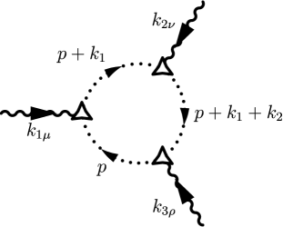
Figure 5: This diagram contains three insertions of the triangle $J$-vertex.

It is easily seen from the Feynman rule of the “triangle” $J$-vertex that this diagram gives a subleading contribution in the low-energy approximation $k_{i}k_{j}\to 0$ and $k_{i}\tilde{k}_{j}$ finite, when compared to the diagrams (4a), (4b) computed so far, hence we will discard its contribution. Summarising, the full three-point function is obtained by adding up the results (4.7) and (4.1).

4.2 The four-point function of background fields

In this section we present the calculation of the four-point function of background fields in the microscopic theory. The computation proceeds in much the same way as that of the three-point function presented in the previous section. For simplicity, we will limit ourselves to the case of gauge group $U(1)$.

As in the three-point function case, only diagrams with at least two insertions of $J$-vertices give a nonvanishing contribution (in the supersymmetric theories we are interested in).

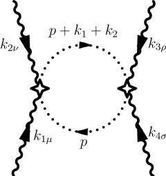
Figure 6: This diagram contains two insertions of the star $J$-vertex.

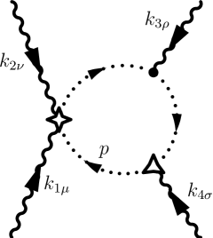
Figure 7: Feynman diagram containing a single insertion of the star and of the triangle $J$-vertex.

Furthermore, terms in the effective action expressions without the functions $P$ or $Q$ (defined in (2.6)) must arise from diagrams containing no powers of external momenta in their vertices. The only such candidates are therefore the diagram shown in figure 6 and its permutations. The expression for this diagram is proportional to:

$$4(\delta^{\mu\sigma}\delta^{\nu\rho}-\delta^{\mu\rho}\delta^{\nu\sigma})\,\mbox{sin}\Bigl{(}\frac{1}{2}k_{1}\tilde{k}_{2}\Bigr{)}\,\mbox{sin}\Bigl{(}\frac{1}{2}k_{3}\tilde{k}_{4}\Bigr{)}\,T(k_{1}+k_{2})\ .$$ (4.21)

We now consider the Feynman diagram in figure 7 (and its permutations). This diagram gives a contribution to the correlator $\Gamma_{\mu\nu\rho\sigma}(k_{1},k_{2},k_{3},k_{4})$ which is proportional to:

$$Q^{4}_{\sigma,\rho\nu}\mbox{sin}\Bigl{(}\frac{1}{2}k_{2}\tilde{k}_{3}\Bigr{)}J_{2}(k_{1},k_{4})\dot{M}_{\mu}(\mu|\tilde{k}_{4}|)+Q^{4}_{\sigma,\rho\mu}\mbox{sin}\Bigl{(}\frac{1}{2}k_{1}\tilde{k}_{3}\Bigr{)}J_{2}(k_{2},k_{4})\dot{M}_{\nu}(\mu|\tilde{k}_{4}|)$$ (4.22)

$$+ Q^{4}_{\sigma,\nu\mu}\mbox{sin}\Bigl{(}\frac{1}{2}k_{1}\tilde{k}_{2}\Bigr{)}J_{2}(k_{3},k_{4})\dot{M}_{\rho}(\mu|\tilde{k}_{4}|)+Q^{3}_{\rho,\nu\mu}\mbox{sin}\Bigl{(}\frac{1}{2}k_{1}\tilde{k}_{2}\Bigr{)}J_{2}(k_{3},k_{4})\dot{M}_{\sigma}(\mu|\tilde{k}_{4}|)$$

$$+ Q^{2}_{\nu,\rho\mu}\mbox{sin}\Bigl{(}\frac{1}{2}k_{1}\tilde{k}_{3}\Bigr{)}J_{2}(k_{2},k_{4})\dot{M}_{\sigma}(\mu|\tilde{k}_{4}|)+Q^{1}_{\mu,\rho\nu}\mbox{sin}\Bigl{(}\frac{1}{2}k_{2}\tilde{k}_{3}\Bigr{)}J_{2}(k_{1},k_{4})\dot{M}_{\sigma}(\mu|\tilde{k}_{4}|)\ .$$

Finally, the remaining diagrams give rise to terms which are proportional to the functions $P^{ij}$ defined in (2.6). In order to calculate these contributions, we need the expressions for a few new integrals. Firstly, we need to consider the integral $L(\sigma,\beta,\gamma)$, defined in (4.1), for the case where $\sigma\neq\beta\neq\gamma$ but $\sigma+\beta+\gamma\neq 0$. We find that:

$$\left[\,L\left(\sigma,\beta,\gamma\right)\,\right]_{\sigma+\beta+\gamma\neq 0}\,=\,\frac{M\left(\mu|\tilde{\sigma}|\right)}{\gamma\tilde{\sigma}}\left(\frac{e^{-i\beta\tilde{\sigma}}-1}{\beta\tilde{\sigma}}+\frac{e^{-i(\beta+\gamma)\tilde{\sigma}}-1}{\left(\beta+\gamma\right)\tilde{\sigma}}\right)\ .$$ (4.23)

It is also necessary to calculate several integrals containing four insertions of propagators. These integrals can be evaluated in a similar way to that used in the the calculation of the integrals appearing in the three-point function calculation. For example, one needs to evaluate, for $\sigma+\beta+\gamma+\delta=0$,

$$L\left(\sigma,\beta,\gamma,\delta\right)= \int\!\!{\frac{d^{4}p}{(2\pi)^{4}}}{\frac{e^{ip\tilde{\sigma}}}{(p^{2}+\mu^{2})[(p+\beta)^{2}+\mu^{2}][(p+\beta+\gamma)^{2}+\mu^{2}][(p+\beta+\gamma+\delta)^{2}+\mu^{2}]}}$$

$$\stackrel{{\scriptstyle\!\!k_{i}k_{j}\to 0}}{{\longrightarrow}}\frac{N(\tilde{\sigma})}{\tilde{\sigma}(\gamma+\delta)}\left[\frac{1-e^{-i\tilde{\sigma}(\beta+\gamma)}}{i\tilde{\sigma}(\beta+\gamma)}\left(\frac{1}{\tilde{\sigma}\delta}+\frac{1}{\tilde{\sigma}\gamma}\right)-\frac{1}{\tilde{\sigma}\delta}-\frac{1-e^{-i\tilde{\sigma}\beta}}{i(\tilde{\sigma}\gamma)(\tilde{\sigma}\beta)}\right],$$ (4.25)

where

$$N(\tilde{\sigma})=\frac{1}{16\pi^{2}}\int^{\infty}_{0}\!d\lambda\,\lambda\,e^{-\lambda\mu^{2}-\frac{\tilde{\sigma}^{2}}{4\lambda}}\ ,$$ (4.26)

and in the last line we have used the low-energy approximation $k_{i}k_{j}\to 0$.

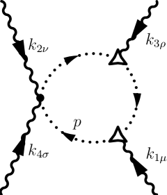
Figure 8: This diagram contains two insertions of the triangle $J$-vertex.

Using such integrals, one sees the emergence of terms proportional to the $J_{2}$- and $J_{3}$-functions defined in (2.9) and (2.11), respectively. We skip the details of the calculation, which is rather lengthy but, for example, the diagram shown in figure 8 produces a term containing $M(\tilde{k}_{4})$ and which turns out to be proportional to the expressions

$$\frac{2}{k_{1}\tilde{k}_{4}}\left[\frac{\mbox{cos}(\frac{1}{2}(k_{1}\tilde{k}_{4}-k_{2}\tilde{k}_{3}))-\mbox{cos}(\frac{1}{2}(k_{1}\tilde{k}_{3}-k_{2}\tilde{k}_{4}))}{k_{3}\tilde{k}_{4}}+\frac{\mbox{cos}(\frac{1}{2}(k_{1}\tilde{k}_{3}+k_{2}\tilde{k}_{4}))-\mbox{cos}(\frac{1}{2}(k_{1}\tilde{k}_{3}-k_{2}\tilde{k}_{4}))}{k_{2}\tilde{k}_{4}}\right]\ .$$ (4.27)

The previous expression (4.27) is precisely equal to $J_{3}(k_{1},k_{2},k_{3})$ defined in (2.11) after imposing $k_{4}=-(k_{1}+k_{2}+k_{3})$.

5 Comparison to the result from the effective action

We are now ready to compare our perturbative results with the expressions for the three- and four-point functions obtained from the effective action $S_{\rm eff}=S^{(1)}_{\rm eff}+S^{(2)}_{\rm eff}$, where $S^{(1)}_{\rm eff}$ and $S^{(2)}_{\rm eff}$ are given in (1.4) and (1.7), respectively.

We begin by considering the three-point function of background gauge fields. In this case, the full perturbative result is obtained by summing up (4.7) with (4.1). We elaborate further these expressions by first performing the sum over the spin $j$. For definiteness, we consider an ${\cal N}=1$ supersymmetric theory with $N_{\rm f}$ adjoint chiral superfields, for which

$$\Bigl{(}\sum_{j}\alpha_{j}\,C(j)\Bigr{)}\,=\,-{1\over 4}(3-N_{\rm f})\ .$$ (5.1)

The case $N_{\rm f}=0$ corresponds to pure ${\cal N}=1$ super Yang-Mills; for $N_{\rm f}=1,3$ we have the ${\cal N}=2$ and ${\cal N}=4$ theories, respectively. Notice that, in the latter case, the contribution to the three-point function vanishes. Secondly, we observe that (4.1) was derived in the low-energy approximation $k_{i}k_{j}\to 0$, with $k_{i}\tilde{k}_{j}$ fixed and finite. We also introduced a small infrared regulating mass $\mu$. In order to compute the corresponding limit of (4.7), we note that this amounts to perform the following modification on the function $T$ of (4.5):

$$T(k)\stackrel{{\scriptstyle\mu}}{{\longrightarrow}}\int\!\!{\frac{d^{4}p}{(2\pi)^{4}}}{\frac{e^{ip\tilde{k}}}{(p^{2}+\mu^{2})[(p+k)^{2}+\mu^{2}]}}\,\stackrel{{\scriptstyle\!\!k^{2}\to 0}}{{\longrightarrow}}\,{\frac{2}{(4\pi)^{2}}}\,K_{0}(\mu|\tilde{k}|)\,\equiv\,S(\mu|\tilde{k}|)\ \ ,$$ (5.2)

where the first arrow stands for equality after introducing the regulator $\mu$ in the expression for $T$, and the second means equality in the limit $k^{2}\to 0$ (at fixed $|k||\tilde{k}|$).

Taking these observations into account, the one-loop perturbative expression for the three-point function, in the low-energy regime $k_{i}k_{j}\to 0$ and $k_{i}\tilde{k}_{j}$ finite, is given by:

$$\Gamma^{ABC}_{\mu\nu\rho}(k_{1},k_{2},k_{3}) = i\sqrt{2N}(N_{\rm f}-3)\,{\sin(k_{2}\tilde{k}_{3}/2)\over k_{2}\tilde{k}_{3}}\ (2\pi)^{4}\delta^{(4)}(k_{1}+k_{2}+k_{3})$$

$$\Bigl{\{}\delta^{A0}\delta^{BC}S(\mu|\tilde{k}_{1}|)\left[\tilde{k}_{1\mu}P_{\rho\nu}^{23}+\tilde{k}_{1{\nu}}P^{13}_{\rho\mu}+\tilde{k}_{1{\rho}}P^{12}_{\nu\mu}+(k_{2}\tilde{k}_{3})\,Q^{1}_{\mu,\nu\rho}\right]$$

$$+\delta^{B0}\delta^{CA}S(\mu|\tilde{k}_{2}|)\left[\tilde{k}_{2{\mu}}P^{23}_{\rho\nu}+\tilde{k}_{2\nu}P_{\rho\mu}^{13}+\tilde{k}_{2{\rho}}P^{12}_{\nu\mu}+(k_{2}\tilde{k}_{3})\,Q^{2}_{\nu,\rho\mu}\right]$$

$$+\delta^{C0}\delta^{AB}S(\mu|\tilde{k}_{3}|)\left[\tilde{k}_{3{\mu}}P^{23}_{\rho\nu}+\tilde{k}_{3{\nu}}P^{13}_{\rho\mu}+\tilde{k}_{3\rho}P_{\nu\mu}^{12}+(k_{2}\tilde{k}_{3})\,Q^{3}_{\rho,\mu\nu}\right]\ .$$

This perturbative result (5) should be contrasted with the result (2.1) (with ${\cal C}=2\alpha_{0}/N$) obtained from the original expression (1.4) for the effective action, where, from the results of [9, 10], it follows that

$$\alpha_{0}\,=\,-4\Bigl{(}\sum_{j}\alpha_{j}C_{j}\Bigr{)}N\,=\,(3-N_{\rm f})N\ ,$$ (5.5)

the sum over $j$ being extended only to fields in the adjoint. The expressions (5) and (1.4) differ in two respect. First, (1.4) contains the function $T$, whereas the perturbative result (5) contains the function $S$. This is easily explained by remembering (5.2), i.e. that at low energy $T\to S$. Second, and more importantly, the perturbative expression (5) contains, in addition to the terms in (2.1), also a contribution proportional to

$$\delta^{A0}\delta^{BC}\,S(\mu|\tilde{k}_{1}|)\,\tilde{k}_{1\mu}P_{\rho\nu}^{23}\,+\,\delta^{B0}\delta^{AC}\,S(\mu|\tilde{k}_{2}|)\,\tilde{k}_{2\nu}P_{\rho\mu}^{13}\,+\,\delta^{C0}\delta^{AB}\,S(\mu|\tilde{k}_{3}|)\,\tilde{k}_{3\rho}P_{\nu\mu}^{12}\ .$$ (5.6)

This new contribution does not arise from the originally conjectured action $S^{(1)}_{\rm eff}$ in (1.4). However, as we have discussed in the introduction, this term (5.6) is precisely reproduced by adding the contribution $S^{(2)}_{\rm eff}$ in (1.7) to the original effective action term in (1.4).

Finally, we consider now the matching of the four-point function obtained from the effective action, Eqs. (2.12) and (2.18), against the perturbative calculation presented in the previous section. We will find that the perturbative calculation is precisely reproduced by the effective action $S_{\rm eff}=S^{(1)}_{\rm eff}+S^{(2)}_{\rm eff}$, where $S^{(1)}_{\rm eff}$ and $S^{(2)}_{\rm eff}$ are the expressions in (1.4) and (1.7).

Feynman diagrams in figure 6 (and its permutations) generate the contribution (4.21), which precisely matches the terms in our expression (2.12) which contains $\delta_{\mu\rho}\delta_{\nu\sigma}$ and no insertions of $P$ and $Q$ functions. Similarly, the first three terms in (4.22) precisely reproduce the terms generated by $S^{(1)}_{\rm eff}$ containing both the $T(k_{4})$ and $Q$ functions. The remaining terms in (4.22) correspond to terms produced by $S^{(2)}_{\rm eff}$ (see (2.18)), when we consider the low-energy limit $\mbox{cos}(\frac{1}{2}k_{i}\tilde{k}_{j})\to 1$ and $\mbox{sin}(\frac{1}{2}k_{i}\tilde{k}_{j})\to\frac{1}{2}k_{i}\tilde{k}_{j}$. Finally, as anticipated in the previous section, combinations of the remaining Feynman diagrams reproduce those terms in $S_{\rm eff}$ that contain the $P$ function.

Summarising, we have a complete agreement between the low-energy limit of the perturbative calculation of three- and four-point functions in the microscopic theory, and the corresponding result obtained from the low-energy effective action $S_{\rm eff}=S^{(1)}_{\rm eff}+S^{(2)}_{\rm eff}$.

References

- [1] A. Connes, M. R. Douglas and A. Schwarz, “Noncommutative geometry and matrix theory: Compactification on tori,” JHEP 9802 (1998) 003, hep-th/9711162.
- [2] M. R. Douglas and C. M. Hull, “D-branes and the noncommutative torus,” JHEP 9802 (1998) 008, hep-th/9711165.
- [3] N. Seiberg and E. Witten, “String theory and noncommutative geometry,” JHEP 9909 (1999) 032, hep-th/9908142.
- [4] C. S. Chu and P. M. Ho, “Constrained quantization of open string in background B field and noncommutative D-brane,” Nucl. Phys. B 568 (2000) 447, hep-th/9906192.
- [5] S. Minwalla, M. Van Raamsdonk and N. Seiberg, “Noncommutative perturbative dynamics,” JHEP 0002 (2000) 020, hep-th/9912072.
- [6] A. Matusis, L. Susskind and N. Toumbas, “The IR/UV connection in the noncommutative gauge theories,” JHEP 0012 (2000) 002, hep-th/0002075.
- [7] M. R. Douglas and N. A. Nekrasov, “Noncommutative field theory,” Rev. Mod. Phys. 73 (2001) 977, hep-th/0106048.
- [8] R. J. Szabo, “Quantum field theory on noncommutative spaces,” Phys. Rept. 378 (2003) 207, hep-th/0109162.
- [9] V. V. Khoze and G. Travaglini, “Wilsonian effective actions and the IR/UV mixing in noncommutative gauge theories,” JHEP 0101 (2001) 026, hep-th/0011218.
- [10] T. J. Hollowood, V. V. Khoze and G. Travaglini, “Exact results in noncommutative N = 2 supersymmetric gauge theories,” JHEP 0105 (2001) 051, hep-th/0102045.
- [11] C. S. Chu, V. V. Khoze and G. Travaglini, “Dynamical breaking of supersymmetry in noncommutative gauge theories,” Phys. Lett. B 513 (2001) 200, hep-th/0105187.
- [12] M. Pernici, A. Santambrogio and D. Zanon, “The one-loop effective action of noncommutative N = 4 super Yang-Mills is gauge invariant,” Phys. Lett. B 504 (2001) 131, hep-th/0011140.
- [13] H. Liu and J. Michelson, “*-TrekK: The one-loop N = 4 noncommutative SYM action,” Nucl. Phys. B 614 (2001) 279, hep-th/0008205.
- [14] D. Zanon, “Noncommutative perturbation in superspace,” Phys. Lett. B 504 (2001) 101, hep-th/0009196.
- [15] A. Santambrogio and D. Zanon, “One-loop four-point function in noncommutative N = 4 Yang-Mills theory,” JHEP 0101 (2001) 024, hep-th/0010275.
- [16] M. Van Raamsdonk, “The meaning of infrared singularities in noncommutative gauge theories,” JHEP 0111 (2001) 006, hep-th/0110093.
- [17] A. Armoni and E. Lopez, “UV/IR mixing via closed strings and tachyonic instabilities,” Nucl. Phys. B 632 (2002) 240, hep-th/0110113.
- [18] S. R. Das and S. J. Rey, “Open Wilson lines in noncommutative gauge theory and tomography of holographic dual supergravity,” Nucl. Phys. B 590 (2000) 453, hep-th/0008042.
- [19] D. J. Gross, A. Hashimoto and N. Itzhaki, “Observables of noncommutative gauge theories,” Adv. Theor. Math. Phys. 4 (2000) 893, hep-th/0008075.
- [20] N. Ishibashi, S. Iso, H. Kawai and Y. Kitazawa, “Wilson loops in noncommutative Yang-Mills,” Nucl. Phys. B 573 (2000) 573, hep-th/9910004.
- [21] H. Liu, “*-Trek II: *n operations, open Wilson lines and the Seiberg-Witten map,” Nucl. Phys. B 614 (2001) 305, hep-th/0011125.
- [22] M. Hayakawa, “Perturbative analysis on infrared and ultraviolet aspects of noncommutative QED on ,” hep-th/9912167.
- [23] L. Jiang and E. Nicholson, “Interacting dipoles from matrix formulation of noncommutative gauge theories,” Phys. Rev. D 65 (2002) 105020, hep-th/0111145.
- [24] Y. j. Kiem, Y. j. Kim, C. Ryou and H. T. Sato, “One-loop noncommutative U(1) gauge theory from bosonic worldline approach,” Nucl. Phys. B 630 (2002) 55, hep-th/0112176.
- [25] R. Britto, B. Feng and S. J. Rey, “Non(anti)commutative superspace, UV/IR mixing and open Wilson lines,” hep-th/0307091.
- [26] N. Seiberg, “Noncommutative superspace, N = 1/2 supersymmetry, field theory and string theory,” JHEP 0306 (2003) 010, hep-th/0305248.
- [27] A. Armoni, “Comments on perturbative dynamics of non-commutative Yang-Mills theory,” Nucl. Phys. B 593 (2001) 229, hep-th/0005208.
- [28] C. P. Martin and D. Sanchez-Ruiz, “The one-loop UV divergent structure of U(1) Yang-Mills theory on noncommutative ,” Phys. Rev. Lett. 83 (1999) 476, hep-th/9903077.
- [29] S. Terashima, “A note on superfields and noncommutative geometry,” Phys. Lett. B 482 (2000) 276, hep-th/0002119.
- [30] J. M. Gracia-Bondia and C. P. Martin, “Chiral gauge anomalies on noncommutative ,” Phys. Lett. B 479 (2000) 321 hep-th/0002171.
- [31] D. J. Gross and N. A. Nekrasov, “Dynamics of strings in noncommutative gauge theory,” JHEP 0010 (2000) 021, hep-th/0007204.
- [32] L. Bonora and M. Salizzoni, “Renormalization of noncommutative U(N) gauge theories,” Phys. Lett. B 504 (2001) 80, hep-th/0011088.
- [33] D. Zanon, “Noncommutative N = 1,2 super U(N) Yang-Mills: UV/IR mixing and effective action results at one loop,” Phys. Lett. B 502 (2001) 265, hep-th/0012009.
- [34] A. Armoni, R. Minasian and S. Theisen, “On non-commutative N = 2 super Yang-Mills,” Phys. Lett. B 513 (2001) 406, hep-th/0102007.
- [35] K. A. Intriligator and J. Kumar, “*-wars episode I: The phantom anomaly,” Nucl. Phys. B 620 (2002) 315, hep-th/0107199.
- [36] C. S. Chu, V. V. Khoze and G. Travaglini, “Notes on noncommutative instantons,” Nucl. Phys. B 621 (2002) 101, hep-th/0108007.
- [37] C. S. Chu, V. V. Khoze and G. Travaglini, “Noncommutativity and model building,” Phys. Lett. B 543 (2002) 318, hep-th/0112139.
- [38] R. Banerjee and S. Ghosh, “Seiberg Witten map and the axial anomaly in noncommutative field theory,” Phys. Lett. B 533 (2002) 162, hep-th/0110177.
- [39] A. Armoni, E. Lopez and S. Theisen, “Nonplanar anomalies in noncommutative theories and the Green-Schwarz mechanism,” JHEP 0206 (2002) 050, hep-th/0203165.
- [40] L. Alvarez-Gaume and M. A. Vazquez-Mozo, “General properties of noncommutative field theories,” hep-th/0305093.
- [41] A. Armoni, E. Lopez and A. M. Uranga, “Closed strings tachyons and non-commutative instabilities,” JHEP 0302 (2003) 020, hep-th/0301099.
- [42] R. Banerjee, “Anomalies in noncommutative gauge theories, Seiberg-Witten transformation and Ramond-Ramond couplings,” hep-th/0301174.
- [43] F. Ardalan and N. Sadooghi, “Planar and nonplanar Konishi anomalies and exact Wilsonian effective superpotential for noncommutative N = 1 supersymmetric U(1),” hep-th/0307155.
- [44] E. Lopez, “From UV/IR mixing to closed strings,”, hep-th/0307196.
- [45] M. E. Peskin and D. V. Schroeder, “An Introduction To Quantum Field Theory,” Addison-Wesley, Reading (1995).
- [46] G. ’t Hooft, “Computation Of The Quantum Effects Due To A Four-Dimensional Pseudoparticle,” Phys. Rev. D 14 (1976) 3432 [Erratum-ibid. D 18 (1978) 2199].