Lab/UFR-HEP0308/GNPHE/0309/IFT-UAM/CSIC-03-28
Classification of $\mathcal{N}\mathbf{=2}$ supersymmetric CFT₄s:
Indefinite Series

Abstract

Using geometric engineering method of $4D$ $\mathcal{N}=2$ quiver gauge theories and results on the classification of Kac-Moody (KM) algebras, we show on explicit examples that there exist three sectors of $\mathcal{N}=2$ infrared CFT₄s. Since the geometric engineering of these CFT₄s involve type II strings on K3 fibered CY3 singularities, we conjecture the existence of three kinds of singular complex surfaces containing, in addition to the two standard classes, a third indefinite set. To illustrate this hypothesis, we give explicit examples of K3 surfaces with H${}_{3}^{4}$ and E₁₀ hyperbolic singularities. We also derive a hierarchy of indefinite complex algebraic geometries based on affine $A_{r}$ and T_(p,q,r) algebras going beyond the hyperbolic subset. Such hierarchical surfaces have a remarkable signature that is manifested by the presence of poles.

Keywords: Geometric engineering of $\mathcal{N}\mathit{=2}$ QFT₄s, Indefinite and Hyperbolic Lie algebras, K3 fibered CY threefolds with indefinite singularities, $\mathcal{N}\mathit{=2}$ CFT₄s embedded in type II strings.

1 Introduction

Recently $D$ dimension supersymmetric conformal field theories (CFT_D ) have been subject to an intensive interest in connection with superstring compactifications on Calabi-Yau (CY) manifolds [1]-[4] and AdS/CFT correspondence [5, 6]. An important class of these super CFTs corresponds to those embedded in type II string compactifications on K3 fibered CY threefolds (CY3) with $ADE$ singularities. These theories admit a very nice geometric engineering [7, 8] in terms of quiver diagrams and are classified into two categories according to the type of K3 singularities: (a) $\mathcal{N}=2$ CFT₄s with gauge group $G=\prod_{i}SU\left(s_{i}n\right)$ and bi-fundamental matters. This category of scale invariant field models is classified by affine $\widehat{ADE}$ Lie algebras. They have vanishing individual beta function $b_{i}$ known to be given by $b_{i}=\frac{1}{12}\left(44n_{i}-\sum_{j}\left[8a_{ij}^{4}+2a_{ij}^{6}\right]n_{j}\right)$ with $a_{ij}^{4}$ and $a_{ij}^{6}$ being the number of Weyl fermions and scalars respectively [2, 9]. In $\mathcal{N}=2$ affine CFT₄s, this beta function relation can be put in the form $b_{i}=\frac{11}{6}\mathbb{K}_{ij}^{\left(0\right)}n_{j}$ and its vanishing condition $\mathbb{K}_{ij}n_{j}=0$ can be solved in terms of the usual Dynkin integer weights $s_{i}$ ($\mathbb{K}_{ij}s_{j}=0$) as follows,

$$\mathbb{K}_{ij}^{\left(0\right)}n_{j}=n\mathbb{K}_{ij}^{\left(0\right)}s_{j}=0,$$ (1)

where $\mathbb{K}_{ij}^{\left(0\right)}$ is the affine $\widehat{ADE}$ Cartan matrix. The extra upper index on $\mathbb{K}_{ij}^{\left(0\right)}$ is introduced for later use. (b) $\mathcal{N}=2$ CFT₄s, based on finite $ADE$ singularities; with gauge group $G=\prod_{i}SU\left(n_{i}\right)$ and matters in both fundamental $\mathbf{n}_{i}$ and bi-fundamental $\left(\mathbf{n}_{i}\mathbf{,}\overline{\mathbf{n}}_{j}\right)$ representations of $G$. In this case, the beta function $b_{i}$ may be put in the form $b_{i}=\frac{11}{6}\left(\mathbb{K}_{ij}^{\left(+\right)}n_{j}-m_{i}\right)$ and so its vanishing condition is equivalent to,

$$\mathbb{K}_{ij}^{\left(+\right)}n_{j}=+m_{i},$$ (2)

where now $\mathbb{K}_{ij}^{\left(+\right)}$ is the finite $ADE$ Cartan matrix and where $m_{i}$ is interpreted as the number of fundamental matters. Here also, we have introduced the extra upper index on $\mathbb{K}_{ij}^{\left(+\right)}$ to distinguish it from $\mathbb{K}_{ij}^{\left(0\right)}$ of eq(1). Note that eq(2) may be thought of as a special deformation of eq(1), which in field theoretic language, consists to add a definite number of Weyl fermions and scalars; that is more supersymmetric fundamental matters. This interpretation is not a new idea in QFT_d; something close to that was already used in the study of deformations of the $2D$ conformal structure; in particular in the analysis of deformations of 2D Toda field theories. In the present $4D$ case, much informations on the deformation of eq(1) to eq(2) and vice versa may be read directly on the explicit relation $b_{i}=\frac{1}{12}\left(44n_{i}-\vartheta_{i}\right)$ with $\vartheta_{i}=\sum_{j}\left[8a_{ij}^{4}+2a_{ij}^{6}\right]n_{j}$. Starting from $b_{i}>0$; that is $44n_{i}>\vartheta_{i}$, one can recover conformal invariance by adding appropriate amount of fundamental matter to the quiver gauge system; this corresponds to increasing $\vartheta_{i}$ until to reach the conformal point. Pushing this reasoning further by remarking that as one may add matter, one may also integrate it out. This corresponds to starting from $b_{i}<0$, i.e $44n_{i}<\vartheta_{i}$ and integrating out some amount of matter which discreases $\vartheta_{i}$. The resulting beta function can be put in the form $\frac{11}{6}\left(\mathbb{K}_{ij}^{\left(-\right)}n_{j}+m_{i}\right)$; so one ends with the following conformal invariant dual formula to eq(2),

$$\mathbb{K}_{ij}^{\left(-\right)}n_{j}=-m_{i};\qquad i=1,....$$ (3)

To give an interpretation to $\mathbb{K}_{ij}^{\left(-\right)}$ matrix, note that the above three eqs show that they are really very remarkable relations in the sense that they may be put altogether into a condensed form as follows

$$\mathbb{K}_{ij}^{\left(q\right)}n_{j}=qm_{i};\qquad q=+1,0,-1.$$ (4)

But this formula is very well known in the literature on KM algebras as it is just the statement of the theorem of their classification which says that the three $q=+1,0,-1$ sectors correspond respectively to finite, affine and indefinite classes of KM algebras [10].

In this paper, we develop the study for the particular class of indefinite $\mathcal{N}=2$ CFT₄s. We will show that this class shares all the basic features we know about finite and affine $\mathcal{N}=2$ QFT₄s and their IR CFT₄ limits embedded in type II string on CY3 with singular K3 fibration. As a consequence of this classification, we conjecture the existence of a third class of local K3s with indefinite singularities; the two others are the known $ADE$ ones. As we usually do in finite and affine standard cases, we will focus our attention here also on the simply laced subset of local K3s classified by indefinite KM algebras and the corresponding mirror geometries. More precisely, we study the special case of $\mathcal{N}=2$ CFT₄ models based on simply laced hyperbolic symmetries as well as particular extensions.

The presentation of this paper is as follows: In section $2$, we review briefly the computation of the general expression of beta function of $\mathcal{N}=2$ QFT₄s using geometric engineering method. Then, we show that the solution for $\mathcal{N}=2$ CFT₄ scale invariance condition coincides exactly with the Lie algebraic classification eq(4). In sections $3$ and $4$, we establish a classification theorem for $\mathcal{N}=2$ CFT₄s and give two explicit illustrating examples. These concern local K3 with hyperbolic H${}_{3}^{4}$ and E₁₀ singularities. In section $5$, we give a conclusion and generalizations.

2 Beta Function in $\mathcal{N}=2$ quiver QFT₄

A nice way to compute the beta function of the $\mathcal{N}=2$ quiver gauge theories is to use the geometric engineering method of QFT₄s embedded in type II strings on CY3 with $ADE$ singularities [7]. This method involves toric representation of CY3, mirror symmetry and techniques of algebraic geometry; in particular trivalent geometry which we review its main lines here below. Details can be found in [7, 8]. To illustrate the idea of the method in a comprehensive way, we start by considering the case of a unique trivalent vertex; then we give the results for chains of trivalent vertices.

Case of one trivalent vertex:   In type IIA string on CY3, a typical trivalent vertex of the toric representation of CY3 is described by the 3-dimensional vectors $V_{i}$,

$$V_{0}=\left(0,0,0\right);\quad V_{1}=\left(1,0,0\right);\quad V_{2}=\left(0,1,0\right);\quad V_{3}=\left(0,0,1\right);\quad V_{4}=\left(1,1,1\right)$$ (5)

satisfying the following toric geometry relation $\sum_{i=0}^{4}q_{i}V_{i}=-2V_{0}+V_{1}+V_{2}+V_{3}-V_{4}=0$. The vector charge $\left(q_{i}\right)=\left(-2,1,1,1,-1\right)$ is known as the Mori vector and the sum of its $q_{i}$ components is zero as required by the CY condition. In type IIB mirror geometry, the $\left(V_{0},V_{1},V_{2},V_{3},V_{4}\right)$ vertices are represented by complex variables $\left(u_{0},u_{1},u_{2},u_{3},u_{4}\right)$ constrained as $\prod_{i}u_{i}^{q_{i}}=1$ and solved by $\left(1,x,y,z,xyz\right)$; see figure 1.

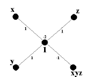
Figure 1: This is a typical trivalent vertex in mirror geometry; It involves a central node and 4 attached ones; 2 of them are of Dynkin type and the others are required by CY  condition. They deal with fundamental matters.

In terms of these variables, the algebraic geometry eq describing mirror geometry is given by the following complex surface, $P\left(X^{\ast}\right)=\mathrm{e}_{0}+\mathrm{a}_{0}x+\mathrm{b}_{0}y+\left(\mathrm{c}_{0}-\mathrm{d}_{0}xy\right)z$, where $\mathrm{a}_{0}\mathrm{,b}_{0}\mathrm{,c}_{0}\mathrm{,d}_{0}$ and $\mathrm{e}_{0}$ are non zero complex moduli. Upon eliminating the $z$ variable by using the eq of motion $\frac{\partial P\left(X^{\ast}\right)}{\partial z}=0$, the above trivalent geometry reduces exactly to

$$P\left(X^{\ast}\right)=\mathrm{a}_{0}x+\mathrm{e}_{0}+\frac{\mathrm{b}_{0}\mathrm{c}_{0}}{\mathrm{d}_{0}}\frac{1}{x},$$ (6)

which is nothing but the mirror of the su$\left(2\right)$ singularity of local K3 surface. To get the eq of the CY3, one promotes the coefficients $\mathrm{a}_{0}\mathrm{,b}_{0}\mathrm{,c}_{0}\mathrm{,d}_{0}$ and $\mathrm{e}_{0}$ to holomorphic polynomials on complex plane as,

$$\mathrm{e}=\sum_{i=0}^{n_{r}}\mathrm{e}_{i}\zeta^{i};\quad\mathrm{a}=\sum_{i=0}^{n_{r-1}}\mathrm{a}_{i}\zeta^{i};\quad\mathrm{b}=\sum_{i=0}^{n_{r+1}}b_{i}\zeta^{i},\quad\mathrm{c}=\sum_{i=0}^{m_{r}}c_{i}\zeta^{i};\quad\mathrm{d}=\sum_{i=0}^{m_{r}^{\prime}}d_{i}\zeta^{i}.$$ (7)

Note that the functions $\mathrm{a,b}$ and $\mathrm{e}$ encode the fibrations of $SU\left(1+n_{r-1}\right)\times SU\left(1+n_{r}\right)\times SU\left(1+n_{r+1}\right)$ gauge symmetry while $\mathrm{c}$ and $\mathrm{d}$ are associated with flavor symmetries of the underlying $\mathcal{N}=2$ QFT₄ engineered over the nodes of the trivalent vertex. The nature of the flavor group will be discussed later on; all what we know about it is that for $m_{r}^{\prime}=0$, the group is $SU\left(1+m_{r}\right)$ but this corresponds to finite class of $\mathcal{N}=2$ CFT₄s. Note also that in geometric engineering method, the $SU\left(1+n_{r}\right)$ and $SU\left(1+n_{r\pm 1}\right)$ gauge symmetries are fibered over $V_{0}$, $V_{1}$ and $V_{2}$. However the two kind of ”matters” $m_{r}$ and $m_{r}^{\prime}$ are fibered over the nodes $V_{3}$ and $V_{4}$ respectively, see figure2.

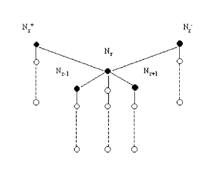
Figure 2: This graph describes a typical vertex one has in geometric engineering of $\mathcal{N}\mathit{=2}$ QFT₄. $SU\left(1+l\right)$ gauge and flavor symmetries are fibered over the five black nodes. Flavor symmetries require large base volume.

Note finally that the holomorphic functions $\mathrm{a,b,c,d}$ and $\mathrm{e}$ are not all of them independent, one can usually fix one of them. We will see that this freedom turns into a condition on $m_{r}$ and $m_{r}^{\prime}$; but for the moment, we keep all these moduli free and make a comment later on.

Infrared $\mathcal{N}=2$ QFT₄ limit:   To get the various $\mathcal{N}=2$ CFT₄s embedded in type IIA strings on CY3, we have to study the infrared field theory limit one gets from mirror geometry eq(6) and look for the scaling properties of the gauge coupling constant moduli. We will do this explicitly for the case of the trivalent vertex and then give the general result for the chain. To that purpose, we proceed in three steps: First determine the behaviour of the complex moduli $\mathrm{f}_{i}$ appearing in the expansion eq(7) under a shift of $\zeta$ by $1/\varepsilon$ with $\varepsilon\rightarrow 0$. Doing this and requiring that eqs(7) should be preserved, that is still staying in the singularity described by eqs(7), we get the following,

$$\mathrm{e}_{l}\sim\varepsilon^{l-n_{r}};\qquad\mathrm{a}_{l}\sim\varepsilon^{l-n_{r-1}};\qquad\mathrm{b}_{l}\sim\varepsilon^{l-n_{r+1}};\qquad\mathrm{c}_{l}\sim\varepsilon^{l-m_{r}};\qquad\mathrm{d}_{l}\sim\varepsilon^{l-m_{r}^{\prime}}.$$ (8)

Second compute the scaling behaviour of the gauge coupling constant moduli $Z^{\left(g\right)}$ under the shift $\zeta^{\prime}=\zeta+1/\varepsilon$. Putting eqs(8) back into the explicit expression of $Z^{\left(g\right)}$ namely $Z^{\left(g\right)}=\frac{a_{0}b_{0}c_{0}}{e_{0}^{2}d_{0}}$, we get the following behaviour $Z^{\left(g_{r}\right)}\sim\varepsilon^{-b_{r}}$ with $b_{r}$ given by,

$$b_{r}=\frac{11}{6}\left[2n_{r}-n_{r-1}-n_{r+1}-\left(m_{r}-m_{r}^{\prime}\right)\right].$$ (9)

This relation tells us: (i) $b_{r}$ is the beta function for the gauge group factor $SU\left(1+n_{r}\right)$. (ii) $b_{r}$ depends on $m_{i}^{\ast}=m_{r}-m_{r}^{\prime}$; it is invariant under global shifts of $m_{r}$ and $m_{r}^{\prime}$, a property which reflects the arbitrariness we have referred to above. Introducing the following notation sing$\left(m_{i}^{\ast}\right)=q$ with $q=+1,0,-1$ respectively associated with the intervals $m_{r}>m_{r}^{\prime}$, $m_{r}=m_{r}^{\prime}$ and  $m_{r}<m_{r}^{\prime}$, we can rewrite eq(9) as $\mathbf{K}_{ij}^{\left(q\right)}n_{j}-q\left|m_{i}^{\ast}\right|$; see also eq(4). Finally taking the limit $\varepsilon\rightarrow 0$, finiteness of $Z^{\left(g\right)}$ requires then that the field theory limit should be asymptotically free; that is $b_{r}\leq 0$. Upper bound $b_{r}=0$ corresponds to scale invariance we are interested in here.

Conformal Invariance phases:   From eq(9) it is not difficult to recognize the three classes of solutions for $\mathbf{K}_{ij}^{\left(q\right)}n_{j}=qm_{i}^{\ast}$: (i) $m_{r}-m_{r}^{\prime}=0$ and $n_{r}=n_{r-1}=n_{r+1}=n$; this corresponds to a generic vertex of $\widehat{SU\left(k\right)}$ affine $\mathcal{N}=2$ conformal CFT₄ with $SU\left(n\right)^{3}$ gauge symmetry. Extension to the other $\widehat{DE}$ geometries is straightforward. (ii) $m_{r}^{\prime}=0$, but the other integers may be taken as $n_{r}=\alpha n;$ $n_{r-1}=\beta n,\ n_{r+1}=\gamma n,$ $m_{r}=\delta n$ with $\alpha,$ $\beta$, $\gamma$, $\delta$ $\in n\mathbb{Z}_{+}$ constrained as $2\alpha=\beta+\gamma+\delta$. As an example, one may take them as $m_{r}=n_{r-1}=n_{r+1}=2n$ and $n_{r}=3n$; this corresponds to a gauge symmetry $SU\left(3n\right)\times SU\left(2n\right)^{2}$ and an $SU\left(2n\right)$ flavor symmetry engineered on the middle vertex of the SU$\left(4\right)$ finite Dynkin diagrams. This solution is also valid for $m_{r}-m_{r}^{\prime}>0$; all one has to do is to substitute the expression of $m_{r}$ of the above solution by $m_{r}^{\ast}$. (iii) For the remarkable case $m_{r}=0$; that is $m_{r}^{\ast}<0$, conformal invariance requires $2n_{r}-n_{r-1}-n_{r+1}+m_{r}^{\prime}=0$ and is solved as $n_{r}=\alpha n;$ $n_{r-1}=\beta n,\ n_{r+1}=\gamma n,$ $m_{r}^{\prime}=\delta^{\prime}n$ with $\alpha,$ $\beta$, $\gamma$, $\delta^{\prime}$ $\in n\mathbb{Z}_{+}$ satisfying $2\alpha+\delta^{\prime}=\beta+\gamma$. As an example, one may take them as $m_{r}^{\prime}=n_{r-1}=n_{r+1}=2n$ and $n_{r}=n$. Note that solutions for conformal invariance may have $m_{r}^{\prime}>n_{r}$ as one sees on the above particular solution. This property constitute one of the arguments we will use to conjecture the flavor symmetry $SU\left(qm_{r}^{\ast}\right)$; it recovers the known results as particular cases. Naturally the $q=-1$ sector corresponds to a new class of solutions. In this regards we will show that this class is linked with simply laced indefinite KM algebras. To do so we need however more than one trivalent vertex since simply laced indefinite Lie algebras have at least a rank four and this corresponds to the over extension of affine $\widehat{A}_{2}$.

Chains of trivalent vertices:   To get the generalization of the above results, it is enough to think about the previous vertices as a generic trivalent vertex of a linear chain of $N$ trivalent vertices, that is

$$V_{0}\rightarrow V_{\alpha}^{0};\qquad V_{3}\rightarrow V_{\alpha}^{+};\qquad V_{4}\rightarrow V_{\alpha}^{-};\qquad V_{1}\rightarrow V_{\alpha-1}^{0};\qquad V_{2}^{0}\rightarrow V_{\alpha+1}^{0},$$ (10)

where $\alpha\in\left\{1,...,N\right\}$. The intersections between $V_{\alpha}^{0}$ and $V_{\alpha\pm 1}^{0}$ are specified by some integers $\mathrm{q}_{\alpha}^{i}$ generally inspired from the Cartan matrix of the KM algebra one is interested in. In this generic case, the data of the toric polytope are fixed by $\sum_{\alpha\geq 0}\left(\mathrm{q}_{\alpha}^{i}V_{\alpha}^{0}+V_{i}^{+}-V_{i}^{-}\right)=0$ and $\sum_{\alpha}^{i}\mathrm{q}_{\alpha}^{i}=0$. Note that the $\pm$ upper indices carried by the $V_{i}^{\pm}$ vertices refer to the fourth $+1$ and five $-1$ entries of the Mori vector $\mathrm{q}_{\tau}^{i}=\left(\mathrm{q}_{\alpha}^{i};+1,-1\right)$ of trivalent vertex. In practice, the Mori vectors $\mathrm{q}_{\alpha}^{i}$s form a $N\times\left(N+s\right)$ rectangular matrix whose $N\times N$ square sub-matrix $q_{j}^{i}$ is minus the generalized Cartan matrix $\mathbb{K}_{ij}^{\left(q\right)}$. For the example of affine $A_{N-1}$, the Mori charges read as $\mathrm{q}_{\alpha}^{i}=2\delta_{\alpha}^{i}-\delta_{\alpha}^{i-1}-\delta_{\alpha}^{i+1}$ with the usual periodicity of affine $\widehat{SU\left(N\right)}$. The remaining $N\times s$ part of $\mathrm{q}_{\alpha}^{i}$ is fixed by the CY condition $\sum_{\alpha}^{i}\mathrm{q}_{\alpha}=0$ and the corresponding vertices are interpreted as dealing with non compact two dimension divisors defining the singular space on which live singularities. In mirror geometry where $x_{\alpha-1},$ $x_{\alpha}$,$\ x_{\alpha+1},\ y_{\alpha},$ and $\frac{x_{\alpha-1}x_{\alpha+1}y_{\alpha}}{y_{\alpha}^{2}}$ are the variables associated with the vertices (10), algebraic eq for a generic vertex extends as a${}_{\alpha-1}x_{\alpha-1}+\mathrm{a}_{\alpha}x_{\alpha}+$a${}_{\alpha+1}x_{\alpha+1}+\mathrm{c}_{\alpha}y_{\alpha}+\mathrm{d}_{\alpha}\frac{x_{\alpha-1}x_{\alpha+1}y_{\alpha}}{x_{\alpha}^{2}}=0$ where $\mathrm{a}_{\alpha}$, $\mathrm{c}_{\alpha}$ and $\mathrm{d}_{\alpha}$ are complex moduli. Summing over the vertices and setting $y_{\alpha}=x_{\alpha}z_{\alpha}$, one gets $P\left(X^{\ast}\right)=\mathrm{a}_{0}x_{0}+$ $\sum_{\alpha\geq 1}\left(\mathrm{a}_{\alpha}x_{\alpha}+\mathrm{c}_{\alpha}x_{\alpha}z_{\alpha}+\mathrm{d}_{\alpha}\frac{x_{\alpha-1}x_{\alpha+1}z_{\alpha}}{x_{\alpha}}\right)$. Eliminating the variable $z_{\alpha}$ as we have done for eq(6), we obtain

$$P\left(X^{\ast}\right)=\sum_{\alpha\geq 0}x^{\alpha}\mathrm{a}_{\alpha}\left(w\right)\prod_{\beta\geq 1}\left(\frac{\mathrm{c}_{\beta}\left(w\right)}{\mathrm{d}_{\beta}\left(w\right)}\right)^{\alpha-\beta}.$$ (11)

From this relation, one gets behaviour $Z^{\left(g_{r}\right)}\sim\varepsilon^{-b_{r}}$ with $b_{r}$ given by,

$$b_{r}^{\left(q\right)}=\frac{11}{6}\left[2n_{r}-n_{r-1}-n_{r+1}-q\left|m_{r}^{\ast}\right|\right];\qquad r=1,.....$$ (12)

3 Classification Theorem of $\mathcal{N}=2$ CFT₄s

Let $\mathcal{G}_{q}$ be some given simply laced Lie algebra of rank r${}_{q}=rank\left(\mathcal{G}_{q}\right)$ and Cartan matrix $\mathbb{K}^{\left(q\right)}$, $corank\left(\mathbb{K}^{\left(q\right)}\right)\leq 1$ and let $q=+1$, $0$ and $-1$ be an integer which refers respectively to the three possible sectors of $\mathcal{G}_{q}$ that is finite, affine and indefinite types. Then the previous results on $\mathcal{N}=2$ quiver gauge CFT₄s can be stated as a theorem to which we shall refer hereafter as the classification theorem of $\mathcal{N}=2$ CFT₄s. As these supersymmetric gauge theories are special limits of underlying 4D massive field theories (QFT₄), we will state this theorem in a more general way.

Theorem:

For any quiver graph $\Delta\left(\mathcal{G}_{q}\right)$ of trivalent vertices with a topology type Dynkin diagram of the simply laced ( finite, affine and indefinite) Lie algebras $\mathcal{G}_{q}$, there corresponds:

(a) A $\mathcal{N}=2$ quiver gauge QFT₄s which is built as usual by extending the geometric engineering method to include indefinite type Dynkin diagrams. They may be denoted as QFT${}_{4}^{\left(q\right)}$

(b) The quiver gauge group of these $\mathcal{N}=2$ QFT${}_{4}^{\left(q\right)}$s is $\prod_{i=1}^{\mathrm{r}_{q}}SU\left(n_{i}\right)$ and the flavor symmetry encoding fundamental matters reads as $\prod_{i=1}^{\mathrm{r}_{q}}SU\left(qm_{i}^{\ast}\right)$. Here, the positive integer $\left|m_{i}^{\ast}\right|$ is the effective number of fundamental matter that contribute to the beta function; it depends on the absolute value of the difference of $m_{i}$ and $m_{i}^{\prime}$.

(c) The $b_{r}$ functions of the $SU\left(n_{i}\right)$ gauge symmetries of these $\mathcal{N}=2$ quiver QFT₄s read as,

$$b_{r}^{\left(q\right)}=\frac{11}{6}\left(\mathbb{K}_{rs}^{\left(q\right)}n_{s}-q\left|m_{r}^{\ast}\right|\right),\qquad r=1,2,...,\mathrm{r}_{q}$$ (13)

where $q$ refers to the the above three mentioned sectors.

(d) In the infrared limit of $\mathcal{N}=2$ gauge quiver QFT₄s where $b_{r}^{\left(q\right)}$ $\ \longrightarrow$ $\ 0$, these theories flow to three classes of 4D $\mathcal{N}=2$ quiver conformal field theories. The flows are in one to one correspondence with the three sectors of $\mathcal{G}_{q}$s. As such $\mathcal{N}=2$ CFT₄s are classified as QFT${}_{4}^{\left(q\right)}$:

(i) Finite $ADE$ $\mathcal{N}=2$ CFT${}_{4}^{+}$s for which the vanishing of the beta function leads to $\mathbb{K}_{rs}^{\left(+\right)}n_{s}=\left|m_{r}^{\ast}\right|$.

(ii) Affine $ADE$ $\mathcal{N}=2$ quiver CFT${}_{4}^{0}$s governed by $\mathbb{K}_{rs}^{\left(0\right)}n_{s}=0$ with one dimension corank$\left(\mathbb{K}_{rs}^{\left(0\right)}\right)$.

(iii) Indefinite $\mathcal{N}=2$ quiver CFT${}_{4}^{-}$s. They are associated with the class $\mathbb{K}_{rs}^{\left(-\right)}n_{s}=-\left|m_{r}^{\ast}\right|$ where now $\mathbb{K}_{rs}^{\left(-\right)}$ is an indefinite Cartan matrix.

To prove this theorem, note that the first three properties follow naturally from the algebraic geometry analysis of the $\mathcal{N}=2$ quiver QFT₄s embedded in type IIA string on CY3 [7, 8] and refs therein. The fourth property (d) of this theorem can be linked to the Vinberg-Kac-Moody basic theorem on the classification of Lie algebras which we recall here below. The property (d) follows from it by setting $u_{i}=n_{i}$ and $v_{i}=\left|m_{r}^{\ast}\right|.$

Vinberg-Kac-Moody Theorem
A generalized indecomposable Cartan matrix $\mathbb{K}$ obey one and only one of the following three statements: (i) Finite type ($\det\mathbb{K}>0$ ): There exist a real positive definite vector $\mathbf{u}$ ($u_{i}>0;$ $i=1,2,...$) such that $\mathbb{K}_{ij}u_{j}=v_{j}>0$. (ii) Affine type, corank$\left(\mathbb{K}\right)=1$, $\det\mathbb{K}=0$: There exist a unique, up to a multiplicative factor, positive integer definite vector $\mathbf{u}$ ($u_{i}>0;$ $i=1,2,...$) such that $\mathbb{K}_{ij}u_{j}=0$. (iii) Indefinite type ($\det\mathbb{K}\leq 0$), corank$\left(\mathbb{K}\right)\neq 1$: There exist a real positive definite vector $\mathbf{u}$ ($u_{i}>0;$ $i=1,2,...$) such that $\mathbb{K}_{ij}u_{j}=-v_{i}<0.$

All the eqs appearing in this theorem combine together to give eq(4). As a consequence of this classification of $\mathcal{N}=2$ CFT${}_{4}^{\left(q\right)}$s, our theorem may also be viewed as a classification of possible K3 singularities. We have then the following,

Corollary

From the property (d) of our classification theorem, we conjecture the existence of indefinite singularities for K3 fibered CY threefolds that are characterized by simply laced indefinite Lie algebras. With this hypothesis, we have: ($\alpha$) Finite $ADE$ singularities; ($\beta$) Affine $\widehat{ADE}$ singularities; ($\gamma$) Indefinite singularities

Note that the above two first singular K3 surfaces are well common in type II strings on CY3. However the third one is a new class which to our knowledge was not studied before. It is dictated from $\mathcal{N}=2$ field theoretic analysis of $\mathcal{N}=2$ CFT${}_{4}^{\left(q\right)}$ possible solutions. In [11], we have made a general analysis of such kind of singularities; here we give explicit illustrating examples. They concern the over extension of affine $\widehat{A}_{2}$ and the over extension of $\widehat{E}_{8}$ respectively baptized as $H_{4}^{3}$ and $E_{10}$.

4 Two Examples of Hyperbolic Singularities

We begin by recalling that mirror geometry of type IIA string on CY3 ($X_{3})$ with affine $\widehat{ADE}$ singularities are conveniently described in algebraic geometry. A typical eq of such geometry is $P\left(X_{3}^{\ast}\right)=\sum_{\alpha}a_{\alpha}y_{\alpha}$, where $X_{3}^{\ast}$ is the mirror of $X_{3}\$ and where $a_{\alpha}=a_{\alpha}\left(w\right)$ are complex moduli with expansion similar to those of eq(7), see also [7]. In this relation, the $y_{\alpha}$ complex variables are constrained as,

$$\prod_{j=1}^{n}y_{j}^{\mathrm{q}_{j}^{i}}=\prod_{\alpha=n+1}^{n+4}y_{\alpha}^{-\mathrm{q}_{\alpha}^{i}},$$ (14)

where $\mathrm{q}_{j}^{i}$ is minus the Cartan matrix $\mathbb{K}_{ij}$ of the corresponding Lie algebra and $y_{\alpha}$, with $n<\alpha<n+5$, are four extra complex variables that are just the monomials appearing in the elliptic curve $\mathrm{E}=y^{2}+x^{3}+z^{6}+\mathrm{\mu}xyz=0$ on which shrinks the affine ADE singularity. Therefore,we have,

$$y_{n+1}=y^{2},\quad y_{n+2}=x^{3},\quad y_{n+3}=z^{6},\quad y_{n+4}=xyz,$$ (15)

where $\left(y,x,z\right)$ are the homogeneous coordinates of the weighted projective space $\mathbf{WP}^{2}\left(3,2,1\right)$. The remaining $n$ complex variables $y_{i}$ definitive the $\widehat{ADE}$ geometry are also solved in terms of the previous $y,x$ and $z$ variables. Such solutions depend on the $\mathrm{q}_{j}^{i}$ and $\mathrm{q}_{\alpha}^{i}$ integer charges forming altogether a $n\times\left(n+4\right)$ rectangular matrix as

$${\large Q}_{\alpha}^{i}=\left(\begin{array}[]{ccccc}\mathrm{q}_{j}^{i},&\mathrm{q}_{n+1}^{i},&\mathrm{q}_{n+2}^{i},&\mathrm{q}_{n+3}^{i},&\mathrm{q}_{n+4}^{i}\end{array}\right).$$ (16)

The resulting two dimensions geometry $y^{2}+x^{3}+z^{6}+\mathrm{\mu}_{0}xyz+\sum_{i=1}^{n}\mathrm{a}_{i}y_{i}=0$ have been studied extensively in the literature for both trivalent and affine geometries. But here we are claiming that such analysis applies as well for the indefinite sector of Lie algebras and deals with the un-explored class of indefinite CFT₄s. As the better thing to justify our claim is to give examples, we will start by recalling some useful features on affine geometries and then study the indefinite case. Before note that the parameter $\mathrm{\mu}$ appearing in the algebraic geometry eq of the elliptic curve E$\left(\mathrm{\mu}\right)$ is its complex structure. It is fixed to a constant $\mathrm{\mu}_{0}$ in the case of affine $ADE$ geometries; but vary in the case indefinite singularities we are interested in here. More precisely, we will see that in the case of simply laced hyperbolic geometries, the parameter $\mathrm{\mu}$ has to vary on a complex plane parameterized by $w$; i.e $\mathrm{\mu=\mu}\left(w\right)$. Under this variation, the initial curve E$\left(\mathrm{\mu}_{0}\right)$ is now promoted to a complex surface E$\left[\mathrm{\mu}\left(w\right)\right]$ which, by the way, is nothing but the elliptic fibration of K3 $y^{2}+x^{3}+z^{6}+\mathrm{\mu}\left(w\right)xyz=0$. Note that, upon appropriate redefinition of variables, one may rewrite the above algebraic geometry eq of the elliptic curve into the following equivalent form,

$$y^{2}+x^{3}+\mathrm{\nu}\left(t\right)z^{\prime 6}+xyz^{\prime}=0$$ (17)

where now $z^{\prime}=\mathrm{\mu}\left(w\right)z$ and $\mathrm{\nu}\left(t\right)z^{\prime 6}=z^{6}$. For instance, if we take $\mathrm{\nu}\left(t\right)=t^{-1}=w^{-6}$, then $z^{\prime}$ should be as $z^{\prime}=wz$ and so $\mathrm{\mu}\left(w\right)=w$. Having these properties in mind, we turn now to illustrate the building of affine A₂ geometry and its hyperbolic over extension.

Affine extension of $\mathbf{A}_{2}$ geometry:   In the special case of affine $A_{2}$ geometry, like all series of affine ADEs, one starts from the curve E${}_{0}=y^{2}+x^{3}+z^{6}+\mathrm{\mu}_{0}xyz=0$ of $\mathbf{WP}^{2}\left(3,2,1\right)$ with fixed complex structure and look for algebraic geometry eq of affine $A_{2}$ geometry which reads as,

$$\widehat{A}_{2}:y^{2}+x^{3}+z^{6}+\mathrm{\mu}_{0}xyz+\left(\mathrm{b}y_{1}+\mathrm{c}y_{2}+\mathrm{d}y_{3}\right)=0.$$ (18)

Here $\mathrm{b},$ $\mathrm{c}$ and $\mathrm{d}$ are complex moduli which once taken simultaneously to zero the affine $A_{2}$ geometry shrinks to the elliptic curve. To get the explicit expression of the remaining $y_{i}$ gauge invariants, one has to specify the toric data for the present affine $A_{2}$ geometry and too particularly the $\mathrm{q}_{j}^{i}$ and $\mathrm{q}_{\alpha}^{i}$ charges appearing in eq(14). These read as,

$${\large Q}\left(\widehat{A}_{2}\right)=\left(\begin{array}[]{ccccccc}-2&1&1&0&0&1&-1\\ 1&-2&1&2&1&0&-3\\ 1&1&-2&0&1&0&-1\end{array}\right).$$ (19)

The simplest solution one gets for the constraint eqs(14 regarding $y_{1}$, $y_{2}$ and $y_{3}$ is $y_{1}=z^{3},$ $y_{2}=xz$ and $\ y_{2}=y$. However this is not unique as there are infinitely many others depending on an extra free complex parameter $v$ as shown here below,

$$y_{1}=z^{3}v,\qquad y_{2}=xzv,\qquad y_{2}=yv,$$ (20)

where $v$ is a homogeneous complex parameter of scaling weight $3$ so that $\left(x,y,z,v\right)$ parameterize the $\mathbf{WP}^{3}\left(3,2,1,3\right)$. Therefore affine $A_{2}$ geometry reads as,

$$\widehat{A}_{2}:y^{2}+x^{3}+z^{6}+\mathrm{\mu}_{0}xyz+v\left(\mathrm{b}z^{3}+\mathrm{c}xz+\mathrm{d}y\right)=0.$$ (21)

From these relation, one may also write down the vertices and the Mori charges of the corresponding  toric polytope; these may be found in [11]. With the relations (18-21) at hand, we are now ready to build our first example of complex surface with an indefinite singularity.

Over extension of affine $\mathbf{A}_{2}$ geometry:   First of all note that the simplest over extension of $\widehat{A}_{2}$ LKM algebra is a simply laced indefinite Lie algebra; it is generally denoted as H${}_{3}^{4}$ according to the Classification of Wanglai Lie ( see also Appendix) and belongs to the so called hyperbolic subset. It has the following $\mathbb{K}\left(H_{3}^{4}\right)$ Cartan matrix

$$\mathbb{K}\left(H_{3}^{4}\right)=\left(\begin{array}[]{cccc}-2&1&0&0\\ 1&-2&1&1\\ 0&1&-2&1\\ 0&1&1&-2\end{array}\right),\qquad\mathbb{Q}\left(H_{3}^{4}\right)=\left(\begin{array}[]{cccccccc}-2&1&0&0&0&0&0&1\\ 1&-2&1&1&0&0&0&-1\\ 0&1&-2&1&3&1&0&-4\\ 0&1&1&-2&0&1&0&-1\end{array}\right)$$ (22)

$\mathbb{Q}\left(H_{3}^{4}\right)$ is the matrix of corresponding Mori vectors to be used later. To get the mirror geometry of a local K3 surface with $H_{3}^{4}$ singularity, we suppose the three following:

(a) Like for Lie algebra structure where $H_{3}^{4}$ appears as an over extension of affine $A_{2}$, we consider that hyperbolic $H_{3}^{4}$ geometry is also an extension of affine $A_{2}$ one. As such we conjecture that the algebraic geometry eq for $H_{3}^{4}$ surface reads as,

$$H_{3}^{4}:y^{2}+x^{3}+\mathrm{\nu}\left(t\right)z^{6}+xyz+\left(\sum_{i=1}^{4}\mathrm{a}_{i}y_{i}\right)=0,$$ (23)

where we have considered an elliptic curve with a varying complex structure. The $\mathrm{a}_{i}$s moduli describe the complex deformation of $H_{3}^{4}$ singularity of the hyperbolic surface and $y_{i}$s are four gauge invariants that should be solved in terms of the $x$, $y$, $z$ and $t$ variables.

(b) The relations (14) used for affine geometries are also valid for simply laced indefinite Lie algebra sector. As such we have, for the present example, the following relations defining the $y_{i}$ gauge invariants for $H_{3}^{4}$ geometry,

$$\prod_{\alpha=1}^{8}y_{\alpha}^{\mathbb{Q}_{\alpha}^{i}}=1;\qquad i=1,2,3,4.$$ (24)

where the $4\times 8$ rectangular matrix $\mathbb{Q}_{\alpha}^{i}$ define the four Mori vectors associated with the hyperbolic $H_{3}^{4}$ geometry eq(22). The property $\sum_{\alpha}\mathbb{Q}_{\alpha}^{i}=0$ reflects just the CY condition of this special local K3 surface.

(c) Once the $\mathrm{a}_{i}$ moduli encoding the complex deformation of hyperbolic $H_{3}^{4}$ surface are taken simultaneously to zero, the $H_{3}^{4}$ geometry shrinks into eq(17). This means that eq(15) should be modified as,

$$y_{n+1}=y^{2},\quad y_{n+2}=x^{3},\quad y_{n+3}=t^{-1}z^{6},\quad y_{n+4}=xyz,$$ (25)

With these tools at hand, one can solve explicitly the remaining four $y_{i}$ gauge invariants in terms of the complex variables $x$, $y$, $z$ and $t$ of $\mathbf{WP}^{2}\left(3,2,1\right)\times\mathbb{C}^{\ast}$. We find,

$$H_{3}^{4}:y^{2}+x^{3}+z^{6}t^{-1}+xyz+\left[\mathrm{a}z^{6}+\mathrm{b}tz^{6}+\mathrm{c}txz^{4}+\mathrm{d}yz^{3}t\right]=0.$$ (26)

This is the relation we have been after; it is the mirror of a complex K3 surface with a hyperbolic $H_{3}^{4}$ singularity. CY3 are obtained as usual by promoting the complex moduli to polynomials depending on an extra complex variable $\zeta$ as $\mathrm{a}_{i}\left(\zeta\right)=\sum_{j=1}^{n_{i}}\mathrm{a}_{ij}\zeta^{j}$, where $n_{i}$ stand for the rank of $U\left(n_{i}\right)$ group symmetries of underlying $4D$ $\mathcal{N}=2$ quiver gauge theories that are embedded in type IIA string on the above CY3 with $H_{3}^{4}$ singularity. Before concluding, let us give two more comments: (i) As these kind of unfamiliar CY manifolds look a little bit unusual, it is interesting to also write down the solutions for the vertices of the toric polytope associated with the CY3 having a $H_{3}^{4}$ singularity. They read as,

$$yxz \longleftrightarrow V_{8}=\left(0,0,0\right),\quad y^{2}\longleftrightarrow V_{5}=\left(0,0,-1\right),\quad x^{3}\longleftrightarrow V_{6}=\left(0,-1,0\right),$$

$$t^{-1}z^{6} \longleftrightarrow V_{7}=\left(-1,2,3\right),\quad z^{6}\longleftrightarrow V_{1}=\left(0,2,3\right),\quad\ tz^{6}\longleftrightarrow V_{2}=\left(1,2,3\right),$$ (27)

$$txz^{4} \longleftrightarrow V_{4}=\left(1,1,2\right),\quad yz^{3}t\longleftrightarrow V_{3}=\left(1,1,1\right).$$

Using these expressions and eq(22), it is not difficult to check that these vertices satisfy the basic toric geometry relations namely $\sum_{\alpha=0}^{8}q_{\alpha}^{i}=0$ and $\sum_{\alpha=0}^{8}q_{\alpha}^{i}V_{\alpha}=0$. (ii) The second comment is to discuss the link between affine $A_{2}$ and hyperbolic $H_{3}^{4}$ geometries. As noted before, $H_{3}^{4}$ Lie algebra is just an extension of affine $A_{2}$ and so one expects that there should be a bridge between the two corresponding geometries. This is what happens indeed. Starting from the algebraic geometry eq(21) of affine $A_{2}$, namely $y^{2}+x^{3}+\mathrm{\nu}_{0}z^{6}+xyz+$ $\left(\mathrm{b}z^{3}+\mathrm{c}xz+\mathrm{d}y\right)v$, and performing the following changes

$$\mathrm{\nu}_{0}{\large\longrightarrow}\mathrm{\nu}\left(t\right)=\mathrm{\alpha}t^{-1}+\mathrm{a},\qquad v{\large\longrightarrow}v=tz^{3},$$ (28)

one gets exactly the hyperbolic $H_{3}^{4}$ mirror geometry of eq(26). Here $\mathrm{\alpha}$ and $\mathrm{a}$ are constants.

Hyperbolic E₁₀ surface:   To start recall that hyperbolic E₁₀ is the simplest over extension of affine $E_{8}$. It is an indefinite KM algebra belonging to the hyperbolic subset, which in Kac notation, reads as T_(p,q,r) with $\left(p,q,r\right)=\left(7,3,2\right)$. Its Cartan matrix $\mathbb{K}\left(E_{10}\right)$ is symmetric and has a negative determinant namely $\det\mathbb{K}\left(E_{10}\right)\mathbb{=-}1$. In 4D $\mathcal{N}=2$ gauge theory embedded in type IIA string, one may geometric engineer the $E_{10}$ hyperbolic QFT₄ models and their infrared CFT${}_{4}^{\left(-\right)}$ limit by considering a local CY3 with an $E_{10}$ singularity as outlined in the classification theorem of section 3. Here we would like to derive $E_{10}$ geometry by using toric geometry methods and local mirror symmetry. Indeed the hypothesis of variation of the complex structure of the elliptic curve allows us to define the hyperbolic $E_{10}$ geometry as,

$$E_{10}:y^{2}+x^{3}+\mathrm{\nu}\left(t\right)z^{6}+xyz+\left(\sum_{i=1}^{10}\mathrm{a}_{i}y_{i}\right)=0,$$ (29)

where $\mathrm{a}_{i}$ are complex moduli and where the ten gauge invariant variables $y_{i}$ are obtained by solving the constraint eqs $\prod_{\alpha=1}^{14}y_{\alpha}^{\mathbb{Q}_{\alpha}^{i}}=1$. Here $\mathbb{Q}_{\alpha}^{i}=\mathbb{Q}_{\alpha}^{i}\left(E_{10}\right)$ are the Mori vectors associated with the hyperbolic $E_{10}$ geometry. $\mathbb{Q}_{\alpha}^{i}$ is a $\left(10+4\right)\times 10$ rectangular matrix whose $10\times 10$ square block is minus $E_{10}$ Cartan matrix. The solution of the constraint eqs $\prod_{\alpha=1}^{14}y_{\alpha}^{\mathbb{Q}_{\alpha}^{i}}=1$ may be obtained without major difficulty as they share features with the product of the A₇, A₃ and A₂ singularities. Straightforward computations lead to the following projective exceptional surface,

$$y^{2}+x^{3}+z^{7}t^{-1}+xyz+\mathrm{a}_{0}t^{6}+\mathrm{a}_{1}t^{4}x+\mathrm{a}_{2}t^{2}x^{2}+\mathrm{b}_{1}yt^{4}+\sum_{s=1}^{6}\mathrm{c}_{s}t^{6-s}z^{s}=0,$$ (30)

where $\left(y,x,z,t\right)$ are complex coordinates of WP_(3,2,1,1). Note that if the $\mathrm{a}_{i}$, $\mathrm{b}_{j}$ and $\mathrm{c}_{k}$ complex moduli are simultaneously taken to zero, one ends with a K3 surface with a hyperbolic $E_{10}$ singularity. Moreover promoting the $\mathrm{a}_{i}$, $\mathrm{b}_{j}$ and $\mathrm{c}_{k}$ moduli to polynomials in an extra complex variable $\zeta$ as in eqs(7), one gets a CY3 with complex deformed $E_{10}$ singularity. The degree of these polynomials define the rank of the gauge quiver group factors, in agreement with our classification theorem of $\mathcal{N}=2$ CFT${}_{4}^{\left(-\right)}$s. In the end of this study, note that, like for $\widehat{A}_{2}$ and more generally $\widehat{A}_{r}$, one may here also define a hierarchy of exceptional geometries; but here these correspond just to the geometries associated with the so called T_(p,q,r) KM algebra. Therefore, this kind of algebraic geometric hierarchies are classified by three positive integers $p$, $q$ and $r$ and the corresponding surfaces are given by,

$$\left(y^{r}t^{6-3r}+x^{q}t^{6-2q}+z^{p}t^{6-p}+xyz\right)+\mathrm{a}_{0}t^{6}+\sum_{s=1}^{p-1}\mathrm{c}_{s}t^{6-s}z^{s}+\sum_{s=1}^{q-1}\mathrm{a}_{s}t^{6-2s}x^{s}+\sum_{s=1}^{r-1}\mathrm{b}_{s}y^{r}t^{6-3r}=0,$$ (31)

where as before $\left(y,x,z,t\right)$ are in WP_(3,2,1,1). From this relation, one may re-discover known geometries obtained in earlier literature on 4D $\mathcal{N}=2$ quiver gauge theories. Particular examples are those associated with finite D_r, finite E_s and affine $E_{s}$ exceptional geometries. These three classes of geometries correspond to those T_(p,q,r) algebras with positive determinant of the Cartan matrices as shown here below,

$$\det\left(\mathbb{K}\left[T_{\left(p,q,r\right)}\right]\right)=pq+pr+qr-pqr\geq 0.$$ (32)

The remaining subset of T_(p,q,r) algebras with $\det\left(\mathbb{K}\left[T_{\left(p,q,r\right)}\right]\right)<0$ corresponds effectively to indefinite geometries; they are described by the rational number $c=\frac{1}{p}+\frac{1}{q}+\frac{1}{r}<1$. The complex projective surfaces with $c\geq 1$ are effectively those given by eq(32).

5 Conclusion

In this paper, we have shown on explicit examples that beta function $b_{i}^{\left(q\right)}$ of $\mathcal{N}=2$ quiver gauge theories carries an extra index $q=1,0,-1$, eq(13). In the infrared limit, these gauge theories flow to three different IR points and so one concludes that there exist in general three sectors of $\mathcal{N}=2$ CFT₄s embedded in type IIA superstring on local CY3s. These sectors are in one to one with the three classes ( finite, affine and indefinite) of simply laced KM algebras. Moreover, as these supersymmetric QFT₄s and their CFT₄ IR limits are linked with singularities of K3 fibered CY3, we have conjectured the existence of three kinds of local K3 surfaces classified by generalized Cartan matrices; one of them has indefinite singularities and the two others are the well known ones. To illustrate this claim, we have given two explicit examples namely singular surfaces having hyperbolic H${}_{3}^{4}$ and E₁₀ degeneracies; also known as the over extensions of affine $A_{2}$ and affine $E_{8}$ respectively. These are given by eqs(26) and(30). Among our results, we have also found that hyperbolic geometries may be deduced from the affine category by varying the complex structure of the elliptic curve on $\mathbb{C}^{\ast}$, see eqs(28). Extending this idea, we have shown the above hyperbolic singularities are in fact just leading elements of a hierarchy of a subset of indefinite singular K3 surfaces obtained by iterative mechanism. For the case of affine $A_{2}$ geometry (21) for instance, one gets upon using eqs(28), the following surface with deformed hyperbolic $H_{3}^{4}$ singularity,

$$H_{3}^{4}:y^{2}+x^{3}+z^{6}t^{-1}+xyz+\left[\mathrm{a}z^{6}+\mathrm{b}tz^{6}+\mathrm{c}txz^{4}+\mathrm{d}yz^{3}t\right]=0.$$ (33)

Repeating this procedure once more, one gets the following singular surface $y^{2}+x^{3}+z^{6}t^{-2}+xyz+$ $\left[\mathrm{a}_{-1}z^{6}t^{-1}+\mathrm{a}z^{6}+\mathrm{b}tz^{6}+\mathrm{c}txz^{4}+\mathrm{d}yz^{3}t\right]=0$. It is classified by the following indefinite Lie algebra of minus generalized Cartan matrix given by,

$$\mathbb{K}\left(H_{3,1}^{4}\right)=\left(\begin{array}[]{ccccc}2&-1&0&0&0\\ -1&2&-1&0&0\\ 0&-1&2&-1&-1\\ 0&0&-1&2&-1\\ 0&0&-1&-1&2\end{array}\right),$$ (34)

where $H_{3,1}^{4}$ stands for the over extension of $H_{3}^{4}$. Here also, one can write down the data of this toric manifold as in eqs(22,27). By successive iterations, one may generalize further this result by constructing the following hierarchy of geometries based on affine $\widehat{A}_{2}$,

$$\widehat{A}_{2,k}:y^{2}+x^{3}+z^{6}t^{-k}+xyz+\sum_{s=1}^{k-1}\mathrm{a}_{-s}t^{-s}z^{6}+\left[\mathrm{a}z^{6}+\mathrm{b}tz^{6}+\mathrm{c}txz^{4}+\mathrm{d}yz^{3}t\right]=0,\quad k=1,...,$$ (35)

where $\widehat{A}_{2,0}$ and $\widehat{A}_{2,1}$ stand respectively for affine $\widehat{A}_{2}$ and $H_{3}^{4}$ and where $\widehat{A}_{2,k}$ with $k>1$ refer for the other hierarchical geometries. Like for T_(p,q,r) hierarchies we have studied here, see eq(31), the relations (35) has also poles in $t$. This is a signature of indefinite geometries.

Acknowledgement 1

This work is supported by Protars III, CNRST, Rabat, Morocco. A.Belhaj is supported by Ministerio de Education cultura y Deporte, grant SB 2002-0036.

6 Appendix: Indefinite Lie algebras

Indefinite Lie algebras are still a mathematical open subject since their classification has not yet been achieved. A subset of these indefinite algebras that is quite well understood includes those known as hyperbolic Lie algebras [10, 12]. According to Wanglai-Li classification, there are $238$ containing the following special list of simply laced ones.

$$\mathcal{H}_{1}^{4},\quad\mathcal{H}_{2}^{4},\quad\mathcal{H}_{3}^{4},\quad\mathcal{H}_{1}^{5},\quad\mathcal{H}_{8}^{5},\quad\mathcal{H}_{1}^{6},\quad\mathcal{H}_{5}^{6},\quad\mathcal{H}_{6}^{6},\quad\mathcal{H}_{1}^{7},$$

$$\mathcal{H}_{1}^{7},\quad\mathcal{H}_{1}^{8},\quad\mathcal{H}_{4}^{8},\quad\mathcal{H}_{5}^{8},\quad\mathcal{H}_{1}^{9},\quad\mathcal{H}_{4}^{9},\quad\mathcal{H}_{5}^{9},\quad\mathcal{H}_{1}^{10},\quad\mathcal{H}_{4}^{10}.$$ (36)

For other applications of hyperbolic Lie algebras in string theory; see [13, 14] and refs therein.

References

- [1] S. Kachru, E. Silverstein, 4d Conformal Field Theories and Strings on Orbifolds, Phys.Rev.Lett. 80 (1998) 4855-4858, hep-th/9802183.
- [2] A. Lawrence, N. Nekrasov, C. Vafa, On Conformal Theories in Four Dimensions, Nucl.Phys. B533 (1998) 199-209,
- [3] S. Katz, A. Klemm, C. Vafa, Geometric Engineering of Quantum Field Theories, Nucl.Phys. B497 (1997) 173-195, hep-th/9803015.
- [4] S. Gukov, C. Vafa, E. Witten CFT’s From Calabi-Yau Four-folds, Nucl.Phys. B584 (2000) 69-108; Erratum-ibid. B608 (2001) 477-478, hep-th/9906070.
- [5] J. M. Maldacena, The Large N Limit of Superconformal Field Theories and Supergravity, Adv.Theor.Math.Phys. 2 (1998) 231-252; Int.J.Theor.Phys. 38 (1999) 1113-1133, hep-th/9711200
- [6] N. Berkovits, C. Vafa, E. Witten, Conformal Field Theory of AdS Background with Ramond-Ramond Flux Authors, JHEP 9903 (1999) 018, hep-th/9902098.
- [7] S. Katz, P. Mayr, C. Vafa, Mirror symmetry and Exact Solution of 4D N=2 Gauge Theories I, Adv.Theor.Math.Phys. 1 (1998) 53-114, hep-th/9706110,
- [8] A. Belhaj, A. Elfallah, E.H. Saidi, on the non simply laced mirror geometry in type II strings, Class.Quant.Grav.17:515-532,2000, Class.Quant.Grav.16:3297-3306,1999, hep-th/0012131.
- [9] E M Sahraoui and E.H Saidi, Type IIB String on pp Wave Orbifolds and =2 Supersymmetric Quiver CFT4s, Lab/UFR-HEP/0309.
- [10] V.G.Kac, Infinite dimensional Lie algebras, third edition, Cambridge University Press (1990).
- [11] M. Ait Ben Haddou, A. Belhaj, E.H. Saidi, Geometric Engineering of N=2 CFT_{4}s based on Indefinite Singularities: Hyperbolic Case, hep-th/0307244.
- [12] W. Zhe-Xian, Intrtoduction to Kac-Moody algebras, World Scientific Singapore (1991).
- [13] T. Damour, M. Henneaux , H. Nicolai, E10 and a ”small tension expansion” of M Theory, Phys.Rev.Lett. 89 (2002) 221601, hep-th/0207267
- [14] P. West, Very Extended and at low levels, Gravity and Supergravity, hep-th/0212291.