THE KINETIC DESCRIPTION OF VACUUM PARTICLE CREATION IN THE OSCILLATOR REPRESENTATION

Abstract

The oscillator representation is used for the non-perturbative description of vacuum particle creation in a strong time-dependent electric field in the framework of scalar QED. It is shown that the method can be more effective for the derivation of the quantum kinetic equation (KE) in comparison with the Bogoliubov method of time-dependent canonical transformations. This KE is used for the investigation of vacuum creation in periodical linear and circular polarized electric fields and also in the case of the presence of a constant magnetic field, including the back reaction problem. In particular, these examples are applied for a model illustration of some features of vacuum creation of electron-positron plasma within the planned experiments on the X-ray free electron lasers.

PACS: 11.10.Ef, 25.75.Dw

1 Introduction

The kinetic description of evolution of particle-antiparticle plasma systems, created from vacuum under action of strong fields, has formed now as an active developing branch of modern relativistic kinetic theory. Initially, the corresponding Schwinger term in the kinetic equation (KE) was introduced on the semi-phenomenological basis [1]. The first attempts to obtain it on the dynamical level were fulfilled in works [2]. The fully dynamical ground KE of such kind was obtained in works [3, 4] in the framework of QED. Later, large efforts were directed to the application of these KEs for the description of pre-equilibrium evolution of quark-gluon plasma, arising after collision of two ultrarelativistic heavy ions [5, 6], as well as of the forming of electron-positron plasma from vacuum in the planned experiments on the X-ray free electron lasers (XFEL) at DESY [7] and SLAC [8].

However, the existing procedures (Bogoliubov transformation method [9] in combination with some specific methods of the kinetic theory [3] and the formalism of the single-time Wigner distribution functions [10, 11, 12]) of the dynamical derivation of the KE for the description of the vacuum tunneling processes are rather complicated and limited (especially for particles with many degrees of freedom). Originally, the kinetic theory of such kind was constructed on the dynamical basis only for the case of charged scalar and Dirac particles (separately [5] and together [6]) in a strong linear polarized space homogeneous time-dependent classical electric field (application of these QED equations to the flux tube model in the theory of ultrarelativistic heavy ion collision may be based on the Abelian projection method [13]). On the other hand, large difficulties are met even by the attempt of the transition from the electric field of linear polarization to an arbitrary one in the framework of the both above mentioned methods.

Having in mind the transition to the description of more realistic systems, we are interested in looking for some alternative, more effective formalism of the derivation of the basic KE of the vacuum creation theory. For this aim, we try here the oscillator (or holomorphic) representation (OR) of quantum field theory [14, 15] as a simple example of the scalar QED with a strong electric field (Sect. 2). This formalism is found very effective in some problem series of the quantum field theory (e.g., [16]). The approach based on the Green’s functions method [17, 18] should be mentioned. This method in combination with the Kadanoff-Baym covariant formalism [19] can lead to some alternative variant of the kinetic description of the vacuum particle creation.

In comparison with Bogoliubov method of time-dependent transformations, the OR leads at once to the diagonal form of the Hamiltonian (the quasi-particle representation [9]) and to the specific operator equations of motion, which are the basic elements for the derivation of the KE [3]. The KE itself is obtained in Sec. 3 for the space homogeneous time-dependent quasi-classical electric field of an arbitrary polarization. As a result of numerical solution of the KE, we show, first of all, that the circular polarized harmonic time-dependent electric field is more effective relatively to vacuum particle creation in comparison with the case of the linear polarized radiation.

A more complicated case is considered in Sec. 4, where vacuum particle creation is investigated in the presence of the time-dependent electric field of linear polarization and the collinear constant magnetic field. We study also the back reaction problem, based on the union of the KE and the regularized Maxwell equation. Since the corresponding generalization of the spinor QED is nontrivial, the examples considered in Sec. 3 and 4 can be used to make some qualitative predictions on the results of the planned vacuum particle creation on the XFEL experiments. Finally, Sec. 5 sums up the results of the work.

We use the metric $g^{\mu\nu}=diag(1,-1,-1,-1)$ and the natural units $\hbar=c=1$.

2 The oscillator representation

We will show as the first step that the holomorphic [20] or the OR [14, 15] leads at once to the quasi-particle representation in the scalar QED with an external field. So we consider here the case of a complex scalar field in some classical space homogeneous time-dependent electric field with 4-potential (in the Hamilton gauge)

$$A^{\mu}(t)=\left(0,A^{1}(t),A^{2}(t),A^{3}(t)\right),$$ (1)

and the corresponding field strength $\vec{E}=-\dot{\vec{A}}$, where the overdot denotes the differentiation with respect to time. This field can be considered either as external field or as the result of mean field approximation based on substitution of the quantized electric field $\tilde{A}^{k}(t)$ with its mean value, $\langle\,\tilde{A}^{k}(t)\,\rangle=A^{k}(t)$, where symbol $\langle\,\ldots\,\rangle$ denotes some averaging operation. In the kinetic theory, taking account of fluctuations leads to collision integrals. Thus, mean field approximation means neglect of dissipative effects.

The Lagrange density

$$\mathcal{L}(x)=D_{\mu}^{*}\varphi^{*}D^{\mu}\varphi-m^{2}\varphi^{*}\varphi$$ (2)

($D_{\mu}=\partial_{\mu}+ieA_{\mu}$, $e$ is particle charge with its sign) leads to the equation of motion

$$(D_{\mu}D^{\mu}+m^{2})\varphi=0.$$ (3)

The space homogeneity of the system allows to look for the solution of the Eq. (3) in the following form

$$\varphi(x)=\int[dp]{\rm e}^{i\vec{p}\,\vec{x}}\varphi(\vec{p},t),$$ (4)

where $[dp]=(2\pi)^{-3/2}d^{3}p$. Then the equation of motion of oscillator type follows from the Eqs. (3) and (4)

$$\ddot{\varphi}^{(\pm)}(\vec{p},t)+\omega^{2}(\vec{p},t)\varphi^{(\pm)}(\vec{p},t)=0$$ (5)

with the time-dependent frequency

$$\omega(\vec{p},t)=\sqrt{m^{2}+\vec{P}^{2}},\qquad\vec{P}=\vec{p}-e\vec{A}.$$ (6)

Symbols $(\pm)$ correspond to positive and negative frequency solutions of the Eq. (5). We suppose a finite limit $\lim\limits_{t\rightarrow-\infty}A^{k}(t)=A^{k}_{-}$ in the infinite past and the solutions $\varphi^{(\pm)}(\vec{p},t)$ become asymptotically free:

$$\varphi^{(\pm)}(\vec{p},t)\mathop{\rightarrow}_{t\rightarrow\,-\infty}{\rm e}^{\pm i\omega_{-}t},\quad\mbox{where}\quad\omega_{-}=\lim\limits_{t\rightarrow\,-\infty}\omega(t).$$ (7)

The Eq. (5) is the starting point of the definition of time-dependent frequency. Now one can introduce the decomposition of the field functions

$$\varphi(x) =\int[dp]\frac{{\rm e}^{i\vec{p}\,\vec{x}}}{\sqrt{2\omega(\vec{p},t)}}\left\{a^{(-)}(\vec{p},t)+b^{(+)}(-\vec{p},t)\right\},$$

$$\varphi^{*}(x) =\int\limits^{\mathstrut}[dp]\frac{{\rm e}^{-i\vec{p}\,\vec{x}}}{\sqrt{2\omega(\vec{p},t)}}\left\{a^{(+)}(\vec{p},t)+b^{(-)}(-\vec{p},t)\right\}$$ (8)

and generalized momenta

$$\pi^{*}(x) =i\int[dp]\sqrt{\frac{1}{2}\omega(\vec{p},t)}{\rm e}^{-i\vec{p}\,\vec{x}}\left\{a^{(+)}(\vec{p},t)-b^{(-)}(-\vec{p},t)\right\},$$

$$\pi(x) =-i\int\limits^{\mathstrut}[dp]\sqrt{\frac{1}{2}\omega(\vec{p},t)}{\rm e}^{i\vec{p}\,\vec{x}}\left\{a^{(-)}(\vec{p},t)-b^{(+)}(-\vec{p},t)\right\}.$$ (9)

The Eqs. (2) and (2) can be obtained from the corresponding decompositions of the free field with the help of formal substitution $\omega(\vec{p})=\sqrt{m^{2}+\vec{p}\,^{2}}\rightarrow\omega(\vec{p},t)$, that is admissible for space homogeneous case.

Thus, the decompositions (2) and (2) are postulated essentially. It is based on the possibility of the introduction of the canonical quantization by the complete analogy with the case of the free field. Indeed, usual commutation relations for the time-dependent creation and annihilation operators

$$\left[a^{(-)}(\vec{p},t),a^{(+)}(\vec{q},t)\right]=\left[b^{(-)}(\vec{p},t),b^{(+)}(\vec{q},t)\right]=\delta(\vec{p}-\vec{q})$$ (10)

etc. follow at once from the canonical commutation relations for the operators $\varphi(x)$ and $\pi(x)$ as a direct consequence of the decompositions (2) and (2).

Another feature of the OR is connected with the diagonal form of the Hamiltonian in the time-dependent occupation number representation: the substitution of the decompositions (2) and (2) to the full energy of the system

$$H_{0}(t)=\int d^{3}x\left\{\pi^{*}\pi+\nabla\varphi^{*}\nabla\varphi+m^{2}\varphi^{*}\varphi\right\}$$ (11)

leads to the following Hamiltonian density in the momentum representation

$$H(\vec{p},t)=\omega(\vec{p},t)\left[a^{(+)}(\vec{p},t)a^{(-)}(\vec{p},t)+b^{(-)}(-\vec{p},t)b^{(+)}(-\vec{p},t)\right]$$ (12)

with $\omega(\vec{p},t)$, defined by the Eq. (6). Thus, the OR leads to the quasiparticle representation with the diagonal Hamiltonian density (12). This way is found more effective in comparison with the ”standard” one based on the procedure of Hamiltonian diagonalization by the time-dependent Bogoliubov transformation (e.g., [9, 21]).

The OR can be a non-perturbative basis for the solution of one particle problem in the strong quasi-classical electric field (1). So let us obtain the equation of motion for the creation and annihilation operators. For this aim, let us also write the action

$$S=\int d^{4}x\left\{\pi^{*}(x)\dot{\varphi}(x)+\pi(x)\dot{\varphi^{*}}(x)-H_{0}(x)\right\}$$ (13)

in this representation

$$S=\int dt\,d^{3}p\biggl{\{}\frac{i}{2}\biggl{(}a^{(+)}(\vec{p},t)\dot{a}^{(-)}(\vec{p},t)-\dot{a}^{(+)}(\vec{p},t)a^{(-)}(\vec{p},t)$$

$$+\dot{b}^{(-)}(\vec{p},t)b^{(+)}(\vec{p},t)-b^{(-)}(\vec{p},t)\dot{b}^{(+)}(\vec{p},t)$$

$$+\Delta(\vec{p},t)\bigl{[}b^{(-)}(\vec{p},t)a^{(-)}(-\vec{p},t)-a^{(+)}(\vec{p},t)b^{(+)}(-\vec{p},t)\bigr{]}\biggr{)}-H_{0}(\vec{p},t)\biggr{\}},$$ (14)

where

$$\Delta(\vec{p},t)=\frac{\dot{\omega}(\vec{p},t)}{\omega(\vec{p},t)}.$$ (15)

The ”anomalous” terms are presented in the Eq.(2) in the square brackets. These terms describe creation and annihilation of the particle-antiparticle pairs with the vacuum transition amplitude (15) under action of the electric field. Then the operator equations of motion [9] follow from that after variations by respect to the amplitudes $a^{(\pm)}$, $b^{(\pm)}$ and subsequent transition to the occupation number representation with the commutation relations (10):

$$\dot{a}^{(\pm)}(\vec{p},t) = \frac{1}{2}\,\Delta(\vec{p},t)b^{(\mp)}(-\vec{p},t)+i\left[H_{0}(t),a^{(\pm)}(\vec{p},t)\right],$$

$$\dot{b}^{(\pm)}(\vec{p},t) = \frac{1}{2}\,\Delta(\vec{p},t)a^{(\mp)}(-\vec{p},t)+i\left[H_{0}(t),b^{(\pm)}(\vec{p},t)\right].$$ (16)

It is assumed that the electric field is switched off in the infinite past

$$\lim\limits_{t\rightarrow-\infty}\vec{E}(t)=-\lim\limits_{t\rightarrow-\infty}\dot{\vec{A}}(t)=0,$$ (17)

but the infinitely distant past and future asymptotics of the vector field can be distinct [9, 21], i.e.

$$\lim\limits_{t\rightarrow-\infty}\vec{A}(t)=\vec{A}_{-}\neq\lim\limits_{t\rightarrow\infty}\vec{A}(t)=\vec{A}_{+}.$$ (18)

Let us also notice that the equations of motion (2) contain some elements of generalization in comparison with the known case [9, 22], where the field polarization remains fixed. This circumstance will be used later on in Sec. 3 in order to derive the KE for the description of vacuum particle creation in the time-dependent electric field of arbitrary polarization. We mark out one feature of the Heisenberg equations of motion (2): each of these equations describes some mixture of positive and negative energy states ( ”non-diagonal” form of equations of motion). That is reflected also in the action (2), where the ”anomalous” contributions $\sim a^{(\pm)}b^{(\pm)}$ are present. In this sense the OR leads to mixed states.

The Eqs. (2) show, that the operator (12) is not a generator of infinitesimal time transformations in the considered Fock space, i.e. it is not the ”proper” Hamiltonian of the system in this representation. However, the action (2) is a homogeneous square form relative to the operators $a^{(\pm)}$ and $b^{(\pm)}$ and its anomalous terms can be eliminated with the help of some special time-dependent Bogoliubov transformation

$$a^{(-)}(\vec{p},t) = \alpha_{\vec{p}}^{*}(t)\,c^{(-)}(\vec{p},t)\ -\beta_{\vec{p}}(t)d^{(+)}(-\vec{p},t),$$

$$b^{(-)}(\vec{p},t) = \alpha_{-\vec{p}}^{*}(t)d^{(-)}(\vec{p},t)-\beta_{-\vec{p}}(t)c^{(+)}(-\vec{p},t)$$ (19)

with the additional relation $|\alpha_{\vec{p}}(t)|^{2}-|\beta_{\vec{p}}(t)|^{2}=1$ (the condition of the transformation reversibility and the form-invariance of the canonical commutation relations (10)). The substitution of the Eqs. (2) into the Eqs. (2) generates to the equations of motion for Bogoliubov coefficients [9, 22]:

$$\dot{\alpha}_{\vec{p}}(t)=\frac{1}{2}\,\Delta(\vec{p},t)\beta^{*}_{\vec{p}}(t){\rm e}^{2i\vartheta(\vec{p};t,t_{0})},\,\,\,\,\,\dot{\beta}_{\vec{p}}(t)=\frac{1}{2}\,\Delta(\vec{p},t)\alpha^{*}_{\vec{p}}(t){\rm e}^{2i\vartheta(\vec{p};t,t_{0})},$$ (20)

where ($t_{0}$ is a field switching on time)

$$\vartheta(\vec{p};t,t_{0})=\int\limits_{t_{0}}^{t}dt^{\prime}\omega(\vec{p},t^{\prime}).$$ (21)

Then the action (2) is transformed to the standard form

$$S=\int dt\,d^{3}p\biggl{\{}\frac{i}{2}\Bigl{[}c^{(+)}(\vec{p},t)\dot{c}^{(-)}(\vec{p},t)-\dot{c}^{(+)}(\vec{p},t)c^{(-)}(\vec{p},t)$$

$$+\,\dot{d}^{(-)}(\vec{p},t)d^{(+)}(\vec{p},t)-d^{(-)}(\vec{p},t)\dot{d}^{(+)}(\vec{p},t)\Bigr{]}-H^{\prime}(\vec{p},t)\biggr{\}},$$ (22)

where the ”true” Hamiltonian $H^{\prime}(\vec{p},t)$ has now a non-diagonal form in the momentum representation (the explicit form of $H^{\prime}(\vec{p},t)$ can be found in [9]). The equations of motion (2) turns into the usual Heisenberg equations, i.e.

$$\dot{c}^{(\pm)}(\vec{p},t)=i\left[H^{\prime}(t),c^{(\pm)}(\vec{p},t)\right],$$ (23)

where the Hamiltonian $H^{\prime}(\vec{p},t)$ is the original point of the theory based on decomposition of the type (2) with the free particle frequency $\omega_{0}(\vec{p})=\sqrt{m^{2}+\vec{p}^{2}}$. Thus, the OR can be considered as the ”turned inside out” Bogoliubov method of the Hamiltonian diagonalization,

On the other hand, the Bogoliubov transformation of the type (2) can be used to restore the diagonal form of the equations of motion (2) without mixing the terms (the first addends) [16]. Then we obtain the following equations of motion in momentum representation:

$$i\dot{\mathcal{A}}^{(\pm)}(\vec{p},t)=\pm\Omega(\vec{p},t)\mathcal{A}^{(\pm)}(\vec{p},t),$$ (24)

where $\mathcal{A}^{(\pm)}(\vec{p},t)$ are creation and annihilation operators in the new representation with some new frequency $\Omega(\vec{p},t)$. These operators allows us to gain the first integral of motion

$$\langle in|\mathcal{A}^{(+)}(\vec{p},t)\mathcal{A}^{(-)}(\vec{p},t)|in\rangle=\langle in|\mathcal{A}^{(+)}(\vec{p},0)\mathcal{A}^{(-)}(\vec{p},0)|in\rangle,$$ (25)

where the averaging procedure is fulfilled over the in-vacuum state. The details connected with that type representation can be found in the work [16]. It is important that the correlator (25) can not be interpreted in quasiparticle terms [9].

3 Particle creation in the time-dependent electric field

As an example, we will obtain the KE describing vacuum scalar particle creation in the electric field (1) of arbitrary polarization. Let us introduce the distribution function of particles using the quasiparticle representation (see Eq.(12)) [9]

$$f(\vec{p},t)=\langle in|a^{(+)}(\vec{p},t)a^{(-)}(\vec{p},t)|in\rangle,$$ (26)

which is related with the distribution function of anti-particles as $\overline{f}(-\vec{p},t)=f(\vec{p},t)$.

Using the method of works [3] and the basic equations of motion (2), it is not difficult to get the KE. Differentiating the distribution function (26), we obtain

$$\dot{f}(\vec{p},t)=\frac{1}{2}\Delta(\vec{p},t)\left[f^{(+)}(\vec{p},t)+f^{(-)}(\vec{p},t)\right],$$ (27)

where the anomalous one-particle correlators are

$$f^{(+)}(\vec{p},t) = \langle in|a^{(+)}(\vec{p},t)\,b^{(+)}(-\vec{p},t)|in\rangle,$$

$$f^{(-)}(\vec{p},t) = \langle in|b^{(-)}(-\vec{p},t)\,a^{(-)}(\vec{p},t)|in\rangle$$ (28)

and the vacuum transition amplitude is

$$\Delta(\vec{p},t)=\frac{e\vec{E}(t)\vec{P}(t)}{\omega^{2}(\vec{p},t)}.$$ (29)

The equations of motion for the functions (3) can be obtained by analogy with the Eq. (27). We write them out in the integral form

$$f^{(\pm)}(\vec{p},t)=\frac{1}{2}\int\limits_{-\infty}^{t}dt^{\prime}\Delta(\vec{p},t^{\prime})\left[1+2f(\vec{p},t^{\prime})\right]e^{\pm 2i\theta(\vec{p};t,t^{\prime})},$$ (30)

where the asymptotic conditions have been introduced

$$\lim_{t\rightarrow-\infty}f^{(\pm)}(\vec{p},t)=0.$$ (31)

The consequence of the Eqs. (27) and (30) is

$$\dot{f}(\vec{p},t)=\Delta(\vec{p},t)Ref^{(+)}(\vec{p},t).$$ (32)

Finally, the substitution of the Eqs. (30) into the Eq. (32) leads to the resulting KE

$$\dot{f}(\vec{p},t)=I(\vec{p},t),$$ (33)

where the function $I(\vec{p},t)$ is the vacuum source term of particles

$$I(\vec{p},t)=\frac{1}{2}\Delta(\vec{p},t)\int\limits_{-\infty}^{t}dt^{\prime}\Delta(\vec{p},t^{\prime})[1+2f(\vec{p},t^{\prime})]\cos[2\,\theta(\vec{p};t,t^{\prime})].$$ (34)

The KE (33), (34) is the non-perturbative result for the electric field (1) in the mean field approximation. The particular case of this KE for the linear polarization was obtained and researched in detail in works [3, 5].

The KE (33) can be transformed to a system of ordinary differential equations, which is convenient for numerical analysis [5] (to compact our formulas here and below, symbols denoting time- and momentum-dependency are dropped in obvious cases)

$$\dot{f} = \frac{1}{2}\Delta v_{1},$$

$$\dot{v}_{1} = \Delta(1+2f)-2\omega v_{2},$$

$$\dot{v}_{2} = 2\omega v_{1},$$ (35)

where $\Delta$ is defined by Eq. (29) and $v_{1}=\frac{1}{2}\mathrm{Re}f^{(+)}$, $v_{2}=\frac{1}{2}\mathrm{Im}f^{(+)}$. The Eqs. (3) must be considered with the zero initial conditions. This equation system has the first integral

$$-(1+2f)^{2}+v_{1}^{2}+v_{2}^{2}=1,$$ (36)

according to it the phase trajectories are located on two-cavity hyperboloid with top coordinates $f=v_{1}=v_{2}=0$ and $f=-1,v_{1}=v_{2}=0$.

Excluding the function $f$ from Eqs. (3), we obtain the two dimensional dynamical system with the equations of motion

$$\dot{v}_{1} = \Delta\sqrt{1+v_{1}^{2}+v_{2}^{2}}-2\omega v_{2},$$

$$\dot{v}_{2} = 2\omega v_{1}^{\phantom{\mathstrut}},$$ (37)

having non-Hamilton structure. This is the direct consequence of unitary nonequivalence between the Heisenberg equations of motion (23) (Hamilton dynamics) and the Heisenberg type equations (2), which is the basis of the KE (33) and the system (3) (non-Hamilton dynamics).

Let us remark also, that the full equation set (3) have no reversal time symmetry but the physical observables are defined by the functions $f,v_{1}$ only, which are not changed at time inversion.

The system (3) is integrated via the Runge-Kutta method with the zero initial conditions $f(\vec{p},t_{0})=v_{1}(\vec{p},t_{0})=v_{2}(\vec{p},t_{0})=0$. The momentum dependence of distribution function is defined by means of digitization of momentum space to 2 or 3-dimensional grid, in each of its node the system (3) is solved. The concrete grid parameters depend on field strength, the typical values are $\Delta p\approx 0.1m$ (grid step) and $p_{max}\approx(10-15)m$ (grid boundary), so the total number of solved equations is of order $10^{5}-10^{6}$.

Now we use the KE (33) to compare the effectiveness of particle creation in the harmonic time-dependent electric field of circular ($\xi=1$) polarization and of linear ($\xi=0$) one (the analog of last case was considered in the spinor QED in works [7])

$$A^{\mu}(t)=(0,0,\xi\chi(t)A\cos{\nu t},\chi(t)A\sin{\nu t}),$$ (38)

where $\chi(t)$ is some function, providing switching on of the field smoothly on a half of the field period (the result does not depend on the explicit form of the switching function when $t\gg 1/\nu$). Time dependence of particle number density

$$n(t)=\int[dp]f(\vec{p},t)$$ (39)

for the fields (38) with the zero initial conditions at $t_{0}=0$ is shown in Fig. 1 (in the natural units). We have chosen the field strength parameter typical for the planned experiments on XFEL [7], but the considerably larger frequency $\nu=0.1m$ (this is convenient for calculation time reduction).

As it follows from Fig. 1, circular polarized field is more effective for vacuum particle creation in comparison with linear polarized field of the same amplitude. The dynamics of particle creation in periodic field changes qualitatively by the increase of the field strength within the range $(0.1-0.5)E_{cr}$, where $E_{cr}=m^{2}/e$. Actually, when $E=0.1E_{cr}$ the time dependence of particle density is periodic with the double frequency and approximately constant mean density value for the period of laser field (Fig. 1, left panel). On the contrary, the mean density increases with time when $E=0.5E_{cr}$ (the density ”accumulation” effect [7], Fig. 1, right panel). This effect is more expressed in the circle polarized field. We prove that for our toy model the creation rate (of charged bosons) in the circle polarized field $\approx$ 4 times larger than that of in the linear polarized field. We think that this proper effect can be valid for the conditions of the planned experiments on the XFEL.

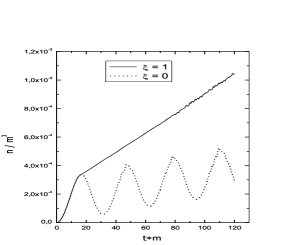
Figure 1: Time dependence of particle number density for the cases of linear and circular polarized field : $E=0.1E_{cr}$ (left panel), $E=0.5E_{cr}$ (right panel). The solid lines correspond to circular polarization ($\xi=1$) and dotted lines correspond to linear one ($\xi=0$).

If the field strength is of the order of critical one, it is necessary to take into account the back reaction of the produced plasma on the primary field. Then the external field $\vec{E}(t)$ should be replaced by the total field

$$\vec{E}(t)=\vec{E}_{in}(t)+\vec{E}_{ex}(t),$$ (40)

where $\vec{E}_{ex}(t)$ is known function and $\vec{E}_{in}(t)$ obeys the Maxwell equation

$$\frac{d\vec{E}_{in}}{dt}=-e\int\limits[dp]\frac{\vec{p}}{\omega}(2f+v_{1}).$$ (41)

The total current density in the r.h.s. of this equation is the sum of conductivity and vacuum polarization currents. Momentum dependency of the functions $f(\vec{p},t)$ and $v_{1}(\vec{p},t)$ is implicit and it is necessary to investigate their ultraviolet behavior in order to fulfill the regularization of the integral (41). The method of the asymptotic expansion can be most adequate one in the framework of the considered non-perturbative formalism. The regularization procedure proposed below is a variant of n-wave regularization technique [24]. Calculation details can be found in the Appendix A. The regularisation in the r.h.s. of the Eq. (41) can be achieved by substitution $v_{1}\to v_{1}-v^{c}_{1}$, where the counter-term $v_{1}^{c}(\vec{p},t)$ is the leading term of the asymptotic series of the function $v_{1}(\vec{p},t)$ over the inverse powers of momentum $|\vec{p}|$

$$v_{1}^{c}(\vec{p},t)=\frac{e\dot{\vec{E}}(t)\vec{p}}{4|\vec{p}|(p^{2}+M^{2})^{3/2}},$$ (42)

where $M$ is an auxiliary mass parameter, $M\gg m$ (some modification of this procedure leads to charge renormalization in the Eq. (41) [28, 29]). The counter terms become significant only in the ultraviolet region. One can choose $M\gg\Lambda$, where $\Lambda$ is a grid boundary of numerical calculation of the integral (41). That allows to omit counter-terms as a negligible quantity. The KE (33) (or the Eqs. (3)) and the Maxwell equation (41) form the complete equation set of the back reaction problem, which have been investigated initially in works [5] for the case of soliton-like pulse of the external linear polarized field. It was shown that the action of the sufficiently strong field $E>E_{cr}$ excites the plasma oscillations with a period, dependent on the residual density after termination of the external pulse. In the considered case $E<E_{cr}$, the density of excited plasma is small and the effects of back reaction are negligible.

4 Magnetic field influence

Now we shall investigate the vacuum creation problem in the case of the collinear time-dependent electric and constant magnetic fields

$$\vec{E}(t)=(0,0,E(t)),\qquad\vec{H}=(0,0,H).$$ (43)

That corresponds to the following configuration of vector potential in the Hamilton gauge

$$A^{\mu}(\vec{x},t)=(0,-Hx_{1},0,A(t)).$$ (44)

Some preliminary results were reported on the conference [25].

In general case, the introduction of the OR is based on the possibility to define the corresponding dispersion law $\omega(\vec{p},t)$ in the presence of the electromagnetic field. This is possible when the spatial and time variables are separable, in particular, for the Klein-Gordon equation (3) in the field (43). That leads to the following solutions

$$\varphi^{(\pm)}_{n,p_{2},p_{3}}(x)=C_{n}T_{n}^{(\pm)}(t)e^{-\eta^{2}/2}H_{n}(\eta)e^{i(p_{2}x_{2}+p_{3}x_{3})}\equiv T_{n}^{(\pm)}(t)\Phi_{n,p_{2},p_{3}}(x),$$ (45)

where $H_{n}(\eta)$ are the Chebyshev-Hermite polynomials, $\eta=\sqrt{|e|H}(x_{1}+p_{2}/|e|H)$ and

$$C_{n}=\frac{1}{2\pi}\left(\frac{1}{\pi}|e|H\right)^{1/4}(2^{n}n!)^{-1/2}$$ (46)

is a normalizing constant. The functions $T_{n}^{(\pm)}(t)$ obey the oscillator-type equation

$$\ddot{T}_{n}^{(\pm)}+\omega_{n}^{2}(t)\,T_{n}^{(\pm)}=0$$ (47)

with the dispersion law ($P=p-eA(t)$, $p=p_{3}$)

$$\omega_{n}^{2}(p,t)=m^{2}+P^{2}+|e|H(2n+1),\;\;n=0,1,...$$ (48)

The symbols $(\pm)$ over the functions $T_{n}^{(\pm)}$ correspond to positive and negative frequency solutions of the Eq. (47) at $t\rightarrow-\infty$ like in Sect. 3. Finally, the solution of of the Eq. (47) satisfies the relation

$$iT_{n}^{*(\pm)}(t)\mathop{\partial_{t}}^{\leftrightarrow}T_{n}^{(\pm)}(t)=\mp 1,$$ (49)

as a consequence of the general orthonormalization condition for the solutions of the Eq. (3)

$$i\int d^{3}x\varphi^{*(\pm)}_{n,p_{2},p}(x)\mathop{\partial_{t}}^{\leftrightarrow}\varphi^{(\pm)}_{n^{\prime},p^{\prime}_{2},p^{\prime}}(x)=\mp\delta_{nn^{\prime}}\delta(p_{2}-p^{\prime}_{2})\delta(p-p^{\prime}).$$ (50)

The oscillator decomposition for the field functions and generalized momenta can be constructed on the basis of the function set (45) by analogy with the Eqs. (2) and (2)

$$\varphi(x)=\sum_{n}\int\frac{dp_{2}dp}{\sqrt{2\omega_{n}(p,t)}}$$

$$\times\left\{a^{(-)}(n,p_{2},p;t)\Phi_{n,p_{2},p}(x)+b^{(+)}(n,p_{2},p;t)\Phi_{n,p_{2},p}^{*}(x)\right\},$$

$$\pi^{*}(x)=i\sum_{n}\int dp_{2}dp\sqrt{\frac{1}{2}\omega_{n}(p,t)}$$

$$\times\left\{a^{(+)}(n,p_{2},p;t)\Phi_{n,p_{2},p}^{*}(x)-b^{(-)}(n,p_{2},p;t)\Phi_{n,p_{2},p}(x)\right\}.$$ (51)

The substitution of the Eqs. (4) into the action (2) leads to the equations of motion

$$\dot{a}^{(\pm)}(n,p_{2},p;t)=\frac{1}{2}W_{n}(p,t)b^{(\mp)}(n,-p_{2},-p;t)+i[H_{0}(t),a^{(\pm)}(n,p_{2},p;t)],$$

$$\dot{b}^{(\pm)}(n,p_{2},p;t)=\frac{1}{2}W_{n}(p,t)a^{(\mp)}(n,-p_{2},-p;t)+i[H_{0}(t),b^{(\pm)}(n,p_{2},p;t)],$$ (52)

where the vacuum transition amplitude is equal

$$W_{n}(p,t)=\frac{|e|E(t)P}{\omega_{n}^{2}(p,t)},$$ (53)

and $H_{0}$ is the Hamiltonian in the diagonal quasiparticle representation with the energy (48). Let us introduce now the new distribution function of scalar particles with momentum $(p_{2},p)$ on the Landau $n$-level

$$f_{n}(p_{2},p,t)=\langle in|a^{(+)}(n,p_{2},p;t)a^{(-)}(n,p_{2},p;t)|in\rangle.$$ (54)

The resulting KE now has the form

$$\dot{f}_{n}(p,t)=\frac{1}{2}W_{n}(p,t)\int\limits_{-\infty}^{t}dt^{\prime}W_{n}(p,t^{\prime})[1+2f_{n}(p,t^{\prime})]\cos\{2\int\limits_{t^{\prime}}^{t}d\tau\omega_{n}(p,\tau)\}.$$ (55)

It was taken into account here that the distribution function does not depend on $p_{2}$ momentum projection $f_{n}(p_{2},p,t)=f_{n}(p,t)$ due to the absence of the $p_{2}$-dependence of the amplitude (53). This is the well known effect of the degeneracy of the observed quantities on the Landau level [26]. We can introduce the effective mass $m^{*}=\sqrt{m^{2}+|e|H}\geq m$ in the Eq. (48), which leads to the increase of the the effective energy gap width and the suppression of vacuum particle creation. This result is in agreement with the known result for a particular case of constant electric and magnetic fields combination [21, 22].

The KE (55) can be reduced to the ordinary differential equation system as in Sect. 3

$$\dot{f}_{n} = \frac{1}{2}W_{n}v_{1n},$$

$$\dot{v}_{1n} = W_{n}(1+2f_{n})-2\omega_{n}v_{2n},$$ (56)

$$\dot{v}_{2n} = 2\omega_{n}v_{1n}.$$

The solution of the back reaction problem is based on the KE (55) and the Maxwell equation (the factor $|e|H$ is the consequence of the above mentioned degeneracy [26])

$$\frac{dE_{in}}{dt}=-2e\frac{|e|H}{(2\pi)^{2}}\sum_{n=0}^{\infty}\int\limits_{-\infty}^{\infty}dp\frac{P}{\omega_{n}(p,t)}\left[f_{n}(p,t)+\frac{1}{2}v_{1n}(p,t)\right].$$ (57)

We investigate the back reaction effect at the presence of the critical magnetic field $H=H_{cr}=m^{2}/e=4.4\cdot 10^{13}Gs$ for the initial electric pulse of the ”rectangular” form

$$E_{ex}(t)=(E_{m}/2)[\tanh(t+b)-\tanh(t-b)]$$ (58)

with the amplitude $E_{m}$ and the duration of $2b$. It is known [9], that constant magnetic field suppress boson creation and enhance fermion creation in the presence of the constant electric field. The situation varies essentially for the case of fast time-dependent electric field. Figs. 2 and 3 show the evolution of the total electric field (40) and particle number density

$$n(t)=\frac{|e|H}{(2\pi)^{2}}\sum_{n=0}^{\infty}\ \int\limits_{-\infty}^{\infty}f_{n}(p,t)\,dp$$ (59)

for the weak and strong electric field with $H=H_{cr}$ and $e^{2}=10$, here $e$ is the effective colour charge (charge value selection is motivated by the flux-tube model in the theory of the QGP generation at ultra-relativistic heavy ion collision [5, 6]). Total field almost coincides with external pulse with $E_{m}=0.1E_{cr}$, i.e. the back reaction is negligible here due to the small particle density. The internal field becomes appreciable when $E_{m}=0.5E_{cr}$ and stable plasma oscillations are excited after the termination of the external pulse. The period of oscillations decreases with the growth of the residual particle density as $\sqrt{n}$. The amplitude of the oscillations becomes large-scale modulated at the further increase of the field, Fig. 3.

Figure 2: Back reaction in the weak electric and strong magnetic field ($H=H_{cr}$): total electric field (left panel), particle number density (right panel). The stable plasma oscillations are excited after termination of the external pulse when $E\geq E_{cr}$.

Figure 3: Back reaction in the strong electric and magnetic field: total electric field (left panel), particle number density (right panel). The plasma oscillations becomes large-scale modulated at the increase of the field to $E\approx E_{cr}$.

During the action of the external pulse (58) with the flat top, particle density grows linearly. The rate value (without the magnetic field) is well approximated with the Schwinger formula for the field strength close to critical value but in the weak field these quantities differ strongly. Analogous situation is for the suppression coefficient of boson creation which is equal to $\sinh{x}/x$ for $E=const$, where $x=\pi H/E$ [9]. For the top plot on Fig. 2 this value is $\approx 2\cdot 10^{11}$, whereas the real difference obtained in the kinetic approach is about 50$\%$.

5 Summary

We have shown on an example of scalar QED, the oscillator (holomorphic) representation is now, apparently, the most effective non-perturbative method for the kinetic description of vacuum particle creation. For an illustration, we have obtained the KE for the case of the arbitrary time-dependent space homogeneous electric field and applied it for a comparison of the effectiveness and other features of vacuum tunneling processes in the linear and circular polarized fields.

Since the corresponding calculations in the spinor QED were not yet fulfilled, these investigations can be the foundation for the qualitative understanding of processes of electron-positron plasma creation in strong laser fields in the planned DESY and SLAC installations. We have investigated also the influence of the magnetic field on vacuum particle creation and have studied the corresponding back-reaction problem, where we have observed great deviations with respect to prediction of the well known results for the case of the constant electric and magnetic fields combination [9, 21].

The results obtained here can be interesting also for the development of the flux-tube model of superconductive type, describing the pre-equilibrium evolution of quark-gluon plasma, generated under conditions of ultrarelativistic heavy ion collisions [27]. The present approach reveals some perspective in the investigation of the dynamics of vacuum particle creation in the strong space homogeneous background fields in more realistic situations when one deals with vacuum creation of particles with inner degrees of freedom (electron-positron, quark-gluon plasma etc.).

Appendix A Regularization procedure

The ultraviolet behavior of the unknown functions $f$, $v_{1}$ and $v_{2}$ is determined by the dispersion law $\omega(\vec{p},t)$ and the vacuum transition amplitude $\Delta(\vec{p},t)$. We can write them out in the spherical coordinate system and define their asymptotic in the ultraviolet region for the electric field (1)

$$\Delta(\vec{p},t)=\frac{e\vec{E}(t)\vec{n}q(t)}{\omega^{2}(q)}\mathop{\longrightarrow}_{q\rightarrow\infty}\frac{e\vec{E}(t)\vec{n}}{q(t)}\sim\frac{1}{q(t)},$$ (A.1)

where $q(t)=\sqrt{\vec{P}^{2}(t)}$ and $\vec{n}=\vec{P}/q$. Now we construct the asymptotic series over the inverse powers of momentum $q$

$$f=\sum_{n=1}f^{(n)},\qquad v_{s}=\sum_{n=1}v_{s}^{(n)},\qquad s=1,2,\;$$ (A.2)

where $f^{(n)}$, $v_{s}^{(n)}\sim q^{-n}$. We get the following leading contributions using these decompositions and the Eqs. (3)

$$f^{(4)}(q,t)=\left(\frac{e\vec{E}(t)\vec{n}}{4q^{2}}\right)^{2}\!,\quad v_{1}^{c}=v_{1}^{(3)}(q,t)=\frac{e\dot{\vec{E}}(t)\vec{n}}{4q^{3}},\quad v_{2}^{(2)}(q,t)=\frac{e\vec{E}(t)\vec{n}}{2q^{2}}.$$ (A.3)

The unique purpose of these counter terms is the elimination of ultraviolet divergence in the integrals defining the densities of physical quantities (e.g., $v_{1}^{c}$ provides the regularization of the electric current in the r.h.s. of the Eq. (41), $f^{(4)}$ - of the energy density etc.). That is why it is necessary to introduce some mechanism of switching on of the counter-terms (A.3) only in the asymptotic region $q\rightarrow\infty$. Switching on the counter terms in the region $q\rightarrow\infty$ can be achieved, e.g., by the replacement of $q^{2}\rightarrow q^{2}+M^{2}$ in the Eqs. (A3), where $M^{2}$ is an auxiliary mass parameter (Pauli-Willars procedure), and trending $M\rightarrow\infty$ after calculations of the integral. Another possibility is to modify the counter terms, e.g.,

$$f_{M}^{(4)}(q,t)=f^{(4)}(q,t)F_{M}(q,t)$$ (A.4)

with the switching function of the type $F_{M}(q,t)=1-\exp(-q/M)$.

When using the computer calculations and therefore introducing the cut-off momentum parameter ($\Lambda=q_{max}$ is a grid boundary), one can always assume counter terms to be negligible small and omit them.

References

-
[1]
E.G. Gurvich, Phys. Lett. B87, 386 (1979);
K. Kajantie and T. Matsui, Phys. Lett. B164, 373 (1985);
G. Gatoff, A.K. Kerman, and T. Matsui, Phys. Rev. D36, 114 (1987);
A. Bialas and W. Chyz, Phys. Rev. D31, 198 (1985); 30, 2371 (1984); Z. Phys. C28, 225 (1985); Nucl. Phys. B267, 242 (1985). -
[2]
J. Rau, Phys. Rev. D50, 6911 (1994);
Y. Kluger, J.M. Eisenberg, B. Svetitsky, F. Cooper, and E. Mottola, Phys. Rev. D45, 4659 (1992). -
[3]
S.A. Smolyansky, G. Röpke, S.M. Schmidt, D. Blaschke,
V.D. Toneev and A.V. Prozorkevich, hep-ph/9712377;
GSI-Preprint-97-92, Regensburg, 1997;
S.M. Schmidt D. Blaschke, G. Röpke, S.A. Smolyansky, A.V. Prozorkevich and V.D. Toneev, Int. J. Mod. Phys. E7, 709 (1998). - [4] Y. Kluger, E. Mottola, and J. M. Eisenberg, Phys. Rev. D58, 125015 (1998).
-
[5]
S.M. Schmidt, D. Blaschke, G. Röpke, A.V. Prozorkevich,
S.A. Smolyansky and V.D. Toneev, Phys. Rev. D59, 094005
(1999);
J. C. Bloch, V. A. Mizerny, A.V. Prozorkevich, C. D. Roberts, S.M. Schmidt, S.A. Smolyansky and D. V. Vinnik, Phys. Rev. D60, 1160011 (1999);
J. C. Bloch, C. D. Roberts, S.M. Schmidt, Phys. Rev. D61, 117502 (2000);
D.V. Vinnik, A.V. Prozorkevich, S.A. Smolyansky, V.D. Toneev, M.B. Hecht, C.D. Roberts, S.M. Schmidt, Eur. Phys. J. C22 341 (2001). - [6] D.V. Vinnik, R. Alkofer, S.M. Schmidt, S.A. Smolyansky, V.V. Skokov and A.V. Prozorkevich, Few-Body Systems, 32, 23 (2002).
-
[7]
J. Andruszkow et al, Phys. Rev. Lett. 85, 3825 (2000);
A. Ringwald, Phys. Lett. B510, 107 (2001); hep-ph/0304139;
R. Alkofer, M.B. Hecht, C.D. Roberts, S.M. Schmidt, and D.V. Vinnik, Phys Rev. Lett. 87, 193902 (2001);
C.D. Roberts, S.M. Schmidt, and D.V. Vinnik, Phys. Rev. Lett. 89, 153901 (2002). -
[8]
C. Bula et al., Phys. Rev. Lett. 76, 3116 (1996);
D.L. Burke et al., ibid, 79, 1626 (1997);
N.B. Narozhnyi and M.S. Fofanov, Zh. Eksp. Teor. Fiz. 117, 476 (2000). - [9] A.A. Grib, S.G. Mamaev and V.M. Mostepanenko, Vacuum Quantum Effects in Strong External Fields, (Friedmann Laboratory Publishing, St. Peterburg, 1994).
- [10] I. Bialynicki-Birula, P. Gornicki, and J. Rafelski, Phys. Rev. D44, 1825 (1991).
- [11] A. Höll, V.G. Morozov, and G. Röpke, quant-ph/0106004; Theor. Math. Phys. 131, 812 (2002); 132, 1026 (2002); quant-ph/0208083.
- [12] A.V. Prozorkevich, S.A. Smolyansky, and S.V. Ilyin, in ”Progress in Nonequilibrium Green’s Functions II”, M. Bonitz and D. Semkat (eds.), (World Scientific Publ., Singapore, 2003), p. 401; hep-ph/0301169.
-
[13]
G.’t-Hooft, Nucl. Phys. B190, 455 (1981);
D.A. Komarov and M.N. Chernodub, JETPh Letters 68, 109 (1998). - [14] G.V. Efimov, Int. J. Mod. Phys. A4, 4977 (1989).
- [15] M. Dineykhan, G.V. Efimov, G. Garbold, and S.N. Nedelko, Lect. Notes Phys. 26, 1 (1995).
- [16] V.N. Pervushin, and V.I. Smirichinski, J. Phys. A: Math. Gen. 32, 6191 (1999).
- [17] E.S. Fradkin, D.M. Gitman, and S.M. Shvartsman, Quantum Electrodynamics with Unstable Vacuum, (Springer-Verlag, Berlin, 1991).
- [18] S.P. Gavrilov and D.M. Gitman, Phys. Rev. D53, 7162 (1996).
- [19] S.A. Smolyansky, A.V. Prozorkevich, G. Maino, and S.G. Mashnik, Ann. Phys. 277, 193 (1999).
- [20] L.D. Faddeev and A.A. Slavnov, Gauge Fields: Introduction to Quantum Theory, (N.-Y., Banjamin-Gummings, 1984).
- [21] A.I. Nikishov, Proc. of the P.N. Lebedev Physical Institute, 111, 152 (Nauka, Moscow, 1979).
- [22] V.S. Popov and M.S. Marinov, Phys. Atom. Nuclei 16, 809 (1972).
-
[23]
G. Gatoff, A.K. Kerman, and T. Matsui,
Phys. Rev. D36, 114 (1987);
M. Asakawa and T. Matsui, Phys. Rev. D43, 2871 (1991). - [24] Ya.B. Zel’dovich and A.A. Starobinskii, Zh. Eksp. Teor. Fiz. 61, 2161 (1971) [Sov. Phys. JETP 34, 1159 (1971)].
- [25] A.V. Tarakanov, A.V. Reichel, S.A. Smolyansky, D.V. Vinnik, and S.M. Schmidt, in ”Progress in Nonequilibrium Green’s Functions II”, M. Bonitz and D. Semkat (eds.), (World Scientific Publ., Singapore, 2003), p. 393.
- [26] L.D. Landau and E.M. Lifschitz, Quantum Mechanics (Non-Relativistic Theory), 3rd ed. (Oxford, England: Pergamon Press, 1977).
- [27] M.A. Lampert and B. Svetitsky, Phys. Rev. D61, 043011 (2000).
- [28] D.V. Vinnik, V.A. Mizerny, A.V. Prozorkevich, S.A. Smolyansky, D.V. Toneev, Preprint JINR P2-2000-85, Dubna (2000).
- [29] Y. Kluger, E. Mottola, and J.M. Eisenberg, Phys. Rev. D58, 125015 (1998).