Stabilization of Extra Dimensions at Tree Level

Abstract

By considering the effects of string winding and momentum modes on a time dependent background, we find a method by which six compact dimensions become stabilized naturally at the self-dual radius while three dimensions grow large.

I Introduction

String theory continues to be a promising candidate for a quantum theory of gravity. However, there are several key challenges in an attempt to relate the theory to phenomenology. One such issue is that string theory predicts a number of extra spatial dimensions. A standard resolution to this problem is to assume that six of the dimensions are small enough to escape experimental detection, which usually means they are taken to be on the order of the Planck scale. Given this, we must not only explain why the six spatial dimensions evolve differently from the other three, but also why they are frozen at such an extraordinarily small size.

A possible resolution to this problem was suggested in bv (see also vafa ) and has since been generalized to include more realistic background geometries and the inclusion of branes extended ; damien ; me . The authors of bv argued that, by considering the dynamics of the winding and momentum modes of the strings, a new symmetry specific of string theory, namely t-duality, could eliminate the big-bang singularity and also explain the dimensionality of space-time. However, these arguments were only qualitative.

In this paper we want to quantify some of the arguments presented in bv . Specifically we will demonstrate that, working in the regime of weak string coupling and at tree level in $\alpha^{\prime}$, we find that the dynamics of string winding and momentum modes lead to a natural mechanism to stabilize the extra dimensions at the self-dual radius.

In Section 2 we will review briefly the origin of the equations of motion for strings in time-dependent backgrounds. These result from demanding conformal invariance of the world-sheet action (vanishing $\beta$ functions). In Section 3 we include the massive modes of the string as source terms for the stringy Einstein equations and demonstrate that the complete set of equations are invariant under t-duality. In Section 4 we solve the equations in the presence of string sources and find that stability of the extra dimensions results naturally for arbitrary initial conditions. We conclude with some brief remarks.

II Dynamics of Strings in Time-Dependent Backgrounds

We begin this section by briefly reviewing the equations of motion for strings in time-dependent backgrounds (for more details see e.g. gsw ). The starting point for strings in a curved space-time is the nonlinear sigma model whose action is

$$S_{\sigma}=-\frac{1}{4\pi\alpha^{\prime}}\int d^{2}\sigma\Bigl{(}\sqrt{-\gamma}\gamma^{ab}G_{\mu\nu}(X)\;\partial_{a}X^{\mu}\partial_{b}X^{\nu}+\epsilon^{ab}B_{\mu\nu}(X)\;\partial_{a}X^{\mu}\partial_{b}X^{\nu}+\alpha^{\prime}\sqrt{\gamma}\phi(X)R^{(2)}\Bigr{)},$$ (1)

where $\gamma^{ab}$ is the world-sheet metric, $(2\pi\alpha^{\prime})$ is the inverse string tension, $G_{\mu\nu}$ is the background space-time metric, $B_{\mu\nu}$ is the background antisymmetric tensor, and $\phi$ is the background dilaton which is coupled to the world-sheet Ricci scalar $R^{(2)}$. The string coupling is given in terms of the dilaton by $g_{s}=e^{2\phi}$.

We obtain the equations of motion by demanding conformal invariance of the world-sheet action. This is equivalent to demanding that the trace of the world-sheet stress tensor given by

$$2\pi T^{a}_{a}=\beta^{G}_{\mu\nu}\sqrt{\gamma}\gamma^{ab}\partial_{a}X^{\mu}\partial_{b}X^{\nu}+\beta^{B}_{\mu\nu}\epsilon^{ab}\partial_{a}X^{\mu}\partial_{b}X^{\nu}+\beta^{\phi}\sqrt{\gamma}R^{(2)},$$ (2)

vanish, where the $\beta$ functions are

$$\beta^{G}_{\mu\nu}=\alpha^{\prime}\Bigl{(}R_{\mu\nu}+2\nabla_{\mu}\nabla_{\nu}\phi-\frac{1}{4}H_{\mu\kappa\sigma}H_{\nu}^{\;\kappa\sigma}\Bigr{)}+{\cal O}(\alpha^{\prime 2}),$$

$$\beta^{B}_{\mu\nu}=\alpha^{\prime}\Bigl{(}\nabla^{\kappa}H_{\kappa\mu\nu}-2\nabla^{\kappa}\phi H_{\kappa\mu\nu}\Bigr{)}+{\cal O}(\alpha^{\prime 2}),$$

$$\beta^{\phi}=\alpha^{\prime}\Bigl{(}\frac{D-26}{3\alpha^{\prime}}-4\nabla_{\kappa}\nabla^{\kappa}\phi+4\nabla_{\kappa}\phi\nabla^{\kappa}\phi-R+\frac{1}{12}H_{\kappa\mu\nu}H^{\kappa\mu\nu}\Bigr{)}+{\cal O}(\alpha^{\prime 2}),$$ (3)

with $H=dB$ denoting the field strength associated with the field $B_{\mu\nu}$. Keeping terms to lowest order in $\alpha^{\prime}$, these equations of motion can alternatively be derived from a low energy effective action formulated in the target space or bulk,

$$S_{bulk}=\frac{1}{4\pi\alpha^{\prime}}\int d^{D}x\sqrt{-G}e^{-2\phi}\Bigl{(}R+4(\nabla\phi)^{2}-\frac{1}{12}H^{2}\Bigr{)}\,,$$ (4)

where $R$ is the Ricci scalar and $G$ is the determinant of the metric. Thus far we have restricted ourselves to the bosonic string, however this action remains valid for the case of the supersymmetric string. For example, with $D=10$ Eq. (4) becomes the low energy effective action of type II-A superstring theory.

We now proceed by demanding that the $\beta$ functions vanish. Assuming that we are in the critical dimension and that there are no fluxes (i.e. $D=26\;or\;10$ and $B_{\mu\nu}=0$) we find that (II) becomes,

$$R_{\mu\nu}+2\nabla_{\mu}\nabla_{\nu}\phi=0,$$

$$R+4\nabla_{\kappa}\nabla^{\kappa}\phi-4\nabla_{\kappa}\phi\nabla^{\kappa}\phi=0.$$ (5)

Next we wish to include stringy sources into the modified Einstein equations (II). This can be done by adding a matter term to the bulk action (4) as was done in vafa . Here we will take a different approach by including the sources at the level of the equations of motion in the form of the stress energy tensor. We expect the equations of motion to generalize in the presence of string sources to

$$R_{\mu}^{\;\;\nu}+2\nabla_{\mu}\nabla^{\nu}\phi=8\pi M^{-2}_{p}\;e^{2\phi}T_{\mu}^{\;\;\nu},$$

$$R+4\nabla_{\kappa}\nabla^{\kappa}\phi-4\nabla_{\kappa}\phi\nabla^{\kappa}\phi=0.$$ (6)

We will assume that the string sources take the form of a perfect fluid,

$$T_{\mu}^{\>\>\nu}=diag(\rho,-p_{1},-p_{2},-p_{3},-p_{4},-p_{5},-p_{6},-p_{7},-p_{8},-p_{9}),$$ (7)

where $\rho$ is the energy density of the strings and $p_{i}$ is the pressure density in the i’th direction.

We conclude this section by consider the equations of motion (II) under the assumption of a homogeneous metric of the form

$$ds^{2}=dt^{2}-e^{2\lambda}d\vec{x}^{2}-e^{2\nu}d\vec{y}^{2},$$ (8)

where $(t,\vec{x})$ are the coordinates of $3+1$ space-time and $\vec{y}$ are the coordinates of the other six dimensions. The scale factors $a(t)$ and $b(t)$ are defined by $\lambda\equiv\ln(a(t))$ and $\nu\equiv\ln(b(t))$.

Given this ansatz for the metric and assuming the string sources to be a perfect fluid, the equations of motion (II) become

$$-3\ddot{\lambda}-3\dot{\lambda}^{2}-6\ddot{\nu}-6\dot{\nu}^{2}+2\ddot{\phi}=\frac{1}{2}e^{2{\phi}}\rho,$$ (10)

$$\ddot{\lambda}+3\dot{\lambda}^{2}+6\dot{\lambda}\dot{\nu}-2\dot{\lambda}\dot{\phi}=\frac{1}{2}e^{2{\phi}}p_{\lambda},$$

$$\ddot{\nu}+6\dot{\nu}^{2}+3\dot{\lambda}\dot{\nu}-2\dot{\nu}\dot{\phi}=\frac{1}{2}e^{2{\phi}}p_{\nu},$$ (12)

$$3\ddot{\lambda}+6\dot{\lambda}^{2}+6\ddot{\nu}+21\dot{\nu}^{2}+18\dot{\lambda}\dot{\nu}+4\dot{\phi}^{2}-4\ddot{\phi}-12\dot{\lambda}\dot{\phi}-24\dot{\nu}\dot{\phi}=0,$$

where $p_{\lambda}$ and $p_{\nu}$ are the pressures in the respective dimensions and we work in Planck units with $16\pi M_{p}^{-2}=e^{2\phi}$.

We note that setting the dilaton to a constant takes our equations to the expected Friedmann-Robertson-Walker (FRW) equations with the constraint $R=0$. Explicitly, if we restrict to the $3+1$ dimensional case ($\nu=0$) we find,

$$H^{2}\equiv\dot{\lambda}^{2}=\frac{8\pi}{3M_{p}^{2}}\rho$$ (13)

$$\ddot{\lambda}+\dot{\lambda}^{2}=-\frac{4\pi}{3M_{p}^{2}}(\rho+3p)$$ (14)

$$R=\ddot{\lambda}+2\dot{\lambda}^{2}=0.$$ (15)

The last condition, $R=0$, implies $T^{\;\;\mu}_{\mu}=0$, which tells us that as the Einstein theory becomes the effective theory the evolution must start in a radiation-like phase with $\rho-3p=0$. This is no surprise since the equations were obtained by demanding conformal invariance. Moreover, this ties the picture together nicely since we expect the stringy effects in cosmology to eventually settle into the radiation dominated phase of the standard cosmological model.

III String Sources and T-duality

In bv it was argued that by considering the dynamics of closed strings on a compact background geometry one could not only produce a nonsingular cosmology, but also provide an explanation for the dimensionality of space-time. The analysis of bv was heuristic but lacked rigorous quantitative calculations. Here we want to address some of the issues in a more quantitative manor (for works addressing other issues more rigorously see vafa ; extended ; damien ; me ). In particular, we will demonstrate that a mechanism to stabilize the extra dimensions can result. Note that a similar investigation of the role of massive string states on the evolution of small and large dimensions was recently published in Borunda . Our results agree with those of Borunda , although the emphasis on the stabilization mechanism is new here.

Closed string theories on a compact geometry have their mass spectrum altered in two ways. First, because the center of mass momentum must be periodic in the compact directions we get its quantization analogous to the Kaluza-Klein case. In addition to these momentum modes there are additional degrees of freedom associated with the possible winding of the strings. These (anti-)winding modes wrap the compact dimensions in a (counter-)clockwise direction. Associated with the winding is a topologically conserved charge known as the winding number. This quantity is (negative) positive for (anti-) winding modes and is conserved so winding modes can only be created and destroyed in pairs. When a winding mode intersects with an anti-winding mode this results in a closed unwound string with winding number zero. The total mass spectrum of the string also includes the oscillatory modes which give rise to the particle spectrum. The spectrum is found by demanding all states to be on-shell and in the case of one compact dimension takes the form Polchinski

$$M^{2}=\frac{n^{2}}{R^{2}}+w^{2}R^{2}+2(N+\tilde{N}-2),$$ (16)

where we have chosen units where $\alpha^{\prime}=1$. The integers $n$ and $w$ denote the Kaluza-Klein level and the winding numbers of the string, respectively. $N$ and $\tilde{N}$ are the left and right oscillators of the string that give rise to the particle spectrum and $R$ is the radius of the compact dimension. It was shown in Kripfganz that the oscillator terms are exponentially suppressed and rendered unimportant for determining the overall evolution of the background. Thus, we will focus on the zero modes of the mass spectrum in the rest of this paper.

The important result that can immediately be seen from (16) is that the spectrum remains unchanged if we send $R\rightarrow 1/R$ and $n\leftrightarrow w$. This property is know as t-duality. It turns out that t-duality is not just a property of the strings, but also of the cosmological background Polchinski_tdual . To see this, we note that the role of the radius is played by the scale factors $a(t)$ and $b(t)$. We then find that the cosmological equations (10)-(12) are invariant under the duality transformation,

$$\lambda(t)\rightarrow-\lambda(t),\;\;\;\;\nu(t)\rightarrow-\nu(t),\;\;\;\;{\phi}(t)\rightarrow{\phi}(t)-3\lambda(t)-6\nu(t).$$ (17)

Shifting the dilaton by the volume factor is required because this is a dynamical (time-dependent) duality.

Now that we have observed that our equations and string sources are duality invariant let us proceed by explicitly constructing energy and pressure terms consisting of the zero modes of the string. From (16) we find that the zero mode energy and pressure of the string gas in $D-1$ compact dimensions can be written as,

$$E=3\mu N^{(3)}e^{\lambda}+3\mu M^{(3)}e^{-\lambda}+6\mu N^{(6)}e^{\nu}+6\mu M^{(6)}e^{-\nu},$$

$$P_{\lambda}=-\mu N^{(3)}e^{\lambda}+\mu M^{(3)}e^{-\lambda},$$

$$P_{\nu}=-\mu N^{(6)}e^{\nu}+\mu M^{(6)}e^{-\nu},$$ (18)

where $\mu$ is the chemical potential (mass per unit length of the string), $E$ is the energy, and $P_{i}$, $N^{i}$, $M^{i}$ are the pressure, number of winding and momentum modes in the ith direction, respectively. By substituting these terms into (10)-(12) we find the equations describing the evolution of our background in terms of string sources,

$$-\ddot{\lambda}-\dot{\lambda}^{2}-2\ddot{\nu}-2\dot{\nu}^{2}+\frac{2}{3}\ddot{\phi}=\frac{\mu}{2}e^{2{\phi}-3\lambda-6\nu}\Bigl{(}N^{(3)}e^{\lambda}+M^{(3)}e^{-\lambda}+2N^{(6)}e^{\nu}+2M^{(6)}e^{-\nu}\Bigr{)}$$ (19)

$$\ddot{\lambda}+3\dot{\lambda}^{2}+6\dot{\lambda}\dot{\nu}-2\dot{\lambda}\dot{\phi}=\frac{\mu}{2}e^{2{\phi}-3\lambda-6\nu}\Bigl{(}-N^{(3)}e^{\lambda}+M^{(3)}e^{-\lambda}\Bigr{)}$$ (20)

$$\ddot{\nu}+6\dot{\nu}^{2}+3\dot{\lambda}\dot{\nu}-2\dot{\nu}\dot{\phi}=\frac{\mu}{2}e^{2{\phi}-3\lambda-6\nu}\Bigl{(}-N^{(6)}e^{\nu}+M^{(6)}e^{-\nu}\Bigl{)}$$ (21)

$$3\ddot{\lambda}+6\dot{\lambda}^{2}+6\ddot{\nu}+21\dot{\nu}^{2}+18\dot{\lambda}\dot{\nu}+4\dot{\phi}^{2}-4\ddot{\phi}-12\dot{\lambda}\dot{\phi}-24\dot{\nu}\dot{\phi}=0.$$ (22)

These equations give us a quantitative way to address the issues first discussed in bv , where it was argued that the winding modes of the strings become more massive as the universe expands, thus preventing the universe from expanding. We can see this through the above equations since the winding modes contribute a negative pressure term and thus a negative effective potential in the equations of motion for $\lambda$ and $\mu$ vafa . Thus, the negative pressure of the winding modes does NOT imply an accelerating phase for the background as it would if the background were described by pure General Relativity.

When considering the initial state to consist of a gas of string winding modes, the dimensionality and isotropy of space-time can be explained as a natural consequence of the dynamics bv ; damien ; me . The strings are initially taken to be in thermal equilibrium and pairs of wound strings are created and annihilated allowing expansion to persist. As the expansion continues the winding modes fall out of equilibrium and the negative pressure of the remaining modes will halt the expansion. This leads to a period of loitering at which time strings in three of the dimensions can find each other and annihilate into loops damien . This leaves three dimensions filled with a gas of string loops with an equation of state resembling ordinary radiation, whereas the other six dimensions remain compact. Therefore, the dimensionality of space-time results from decompactification of three dimensions, since this is the maximum number of dimensions that strings are able to find each other to intersect.

There are several points of concern with the above argument. As the three dimensions grow large the strings that have not yet annihilated and the strings in the six small dimensions could play an important role in the dynamics. Considering the effect that these inhomogeneities have on the geometry and stability of the model is important for the success of the model and is currently being examined watson . Another important issue is the stability of the internal dimensions. In the above argument it was assumed that the dimensions are trying to expand, but we must also consider the case of contraction. This is where the momentum modes play an important role in the dynamics. As mentioned above, the momentum modes are dual to the winding modes and result in the opposite dynamical behavior. That is, as the universe collapses these modes become heavy and it becomes energetically favored to re-expand. In this way the momentum modes prevent collapse to a singularity by contributing an increasing positive pressure to drive the evolution towards expansion. Thus, the resulting cosmology is non-singular.

Considering both the winding and momentum modes suggests that the natural size of the universe should be at the self-dual radius where the total energy is minimized. At this radius the negative pressure of the winding modes is exactly canceled by the positive pressure of the momentum modes. Thus, in the context of string theory it is natural to expect the evolution of our universe to begin at the self-dual radius, which is unity in string units. In fact, this radius is a very special radius in string theory and represents a point of enhanced symmetry for the gauge groups associated with the internal dimensions and the strings (c.f. johnson ).

An important point that we have not yet discussed is the role of the dilaton. Recall that the string coupling is given by $g_{s}=e^{2\phi}$, where $\phi$ is the dilaton. In order for the equations of motion (19)-(22) to remain valid we must restrict the phase space to the region of small string coupling ($g_{s}<<1$). Moreover, we must choose initial conditions that do not result in a rapidly growing coupling. In our analysis we simply enforce this as an energetically favored constraint. Moreover, a more complete analysis would consider a potential for the dilaton. This would allow us to take our considerations out of the stringy regime and into the classical FRW radiation dominated universe. The potential of the dilaton should be provided by the correct model of supersymmetry breaking (this remains one of the outstanding challenges for string theory).

IV Stabilization

It was shown in damien and me that the equations of motion (19)-(22) lead to a period of cosmological loitering, allowing winding modes to annihilate in three dimensions and resulting in those three dimensions expanding to a large size. However, in these approaches it was assumed that the effect of the six small dimensions could be ignored. Here we improve on this analysis and include the evolution of the small dimensions as well as the gravitational coupling between the large and the small dimensions.

We are interested in Eqs. (19)-(22) in the case when three of the spatial dimensions are taken to be large, expanding, and filled with momentum modes only, i.e. $N^{(3)}=0$, since the winding modes have all annihilated into string loops. The other six dimensions are taken to start at the self-dual radius, i.e. $b=1$ and ${\dot{b}}=0$ in string units. This implies $\nu=\dot{\nu}=\ddot{\nu}=0$, and thus it follows from (21)

$$\ddot{\nu}+6\dot{\nu}^{2}+3\dot{\lambda}\dot{\nu}-2\dot{\nu}\dot{\phi}=0=\frac{\mu}{2}e^{2{\phi}-3\lambda-6\nu}\Bigl{(}-N^{(6)}e^{\nu}+M^{(6)}e^{-\nu}\Bigl{)},$$ (23)

that the pressure must vanish, which is only possible if

$$N^{(6)}\,=\,M^{(6)}\,.$$ (24)

This is an expected result, since at the self-dual point the momentum modes and winding modes should be equivalent.

Given the constraint (24) (and making use of the notation $l(t)=\dot{\lambda}$, $q(t)=\dot{\nu}$, and $f(t)=\dot{\phi}$) we can rewrite the system (19)-(22) as the following system of first order differential equations,

$$7l^{2}+35q^{2}+42lq+\frac{4}{3}f^{2}-10lf-20qf$$

$$\;\;\;\;\;\;\;\;=\mu e^{2\phi-3\lambda-6\nu}\Bigl{(}5M^{(3)}e^{-\lambda}+8N^{(6)}\cosh(\nu)-3N^{(6)}\sinh(\nu)\Bigr{)}$$ (25)

$$\dot{f}=-\frac{15}{4}q^{2}-\frac{9}{2}lq-3qf-\frac{3}{4}l^{2}-\frac{3}{2}lf+f^{2}$$

$$\;\;\;\;\;\;\;\;+\frac{3\mu}{4}e^{2\phi-3\lambda-6\nu}\Bigl{(}\frac{1}{2}M^{(3)}e^{-\lambda}-2N^{(6)}\sinh(\nu)\Bigr{)}$$ (26)

$$\dot{l}=-3l^{2}-6lq+2lf+\frac{\mu}{2}M^{(3)}e^{2\phi-4\lambda-6\nu}$$ (27)

$$\dot{q}=-6q^{2}-3lq+2qf-\mu N^{(6)}e^{2\phi-6\nu-3\lambda}\sinh(\nu).$$ (28)

We take (IV) as a constraint on the initial data and then solve the remaining system numerically.

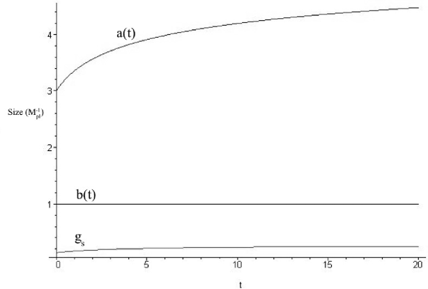
Figure 1: Here we take the six small dimensions to be at the self-dual radius and with vanishing expansion rate initially, $b_{0}=1$ and $\dot{\nu}_{0}=0$. We find that the dimensions remain stable at the self-dual point regardless of the behavior of the dilaton and of the three large dimensions. These are shown in the figure for the initial values $\lambda_{0}=3$, $\dot{\lambda}_{0}=0.5$, and $\phi_{0}=-3$. However, this result holds for generic initial values as long as we respect the weak coupling limit (i.e. $g_{s}<<1$). Note that we are using Planck units.

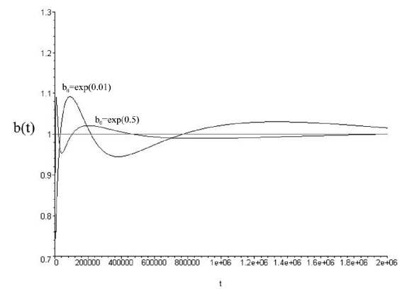
Figure 2: We consider initial values of $b(t)$ away from the self-dual radius and find oscillations about the self-dual radius which are damped by the dilaton and by the evolution of the large dimensions. This is again a generic result. Here we present the evolution for the following initial data: $\dot{\lambda}_{0}=.500,\phi_{0}=-3.00,\dot{\phi}_{0}=.380,\lambda_{0}=3.00,\dot{\nu}_{0}=0,\nu_{0}=0$
$\dot{\lambda}_{0}=.500,\phi_{0}=-3.00,\dot{\phi}_{0}=-.020,\lambda_{0}=3.00,\dot{\nu}_{0}=-.100,\nu_{0}=.010$
$\dot{\lambda}_{0}=.500,\phi_{0}=-3.00,\dot{\phi}_{0}=-.008,\lambda_{0}=3.00,\dot{\nu}_{0}=-.100,\nu_{0}=.500$

We first consider the six small dimensions to be initially static at the self-dual radius. We find that they remain fixed and stable at the self-dual radius for all subsequent times. This result is robust and independent of the behavior of the three large spatial dimensions and the dilaton. In Fig. (1) we plot (in Planck units) the behavior of the two scale factors and of the string coupling as a function of time. As can be seen from the figure, the string coupling remains small for all times guaranteeing that the weak coupling regime is valid.

We now relax our assumption that the small dimensions begin at the self-dual point (maintaining, however, the constraint (24)). In this way we can examine whether the winding and momentum modes do indeed drive the system towards the self-dual point. We begin by introducing an initial radius slightly larger than the self-dual radius and consider the evolution with a nonzero expansion rate. At the beginning of the evolution, $b(t)$ oscillates around the self-dual radius with decreasing amplitude as can be seen in Fig. (2). The dilaton and the three other dimensions play an important role by damping the oscillations. It is important to note that the damping is not dependent on the dilaton alone, as can be seen from the exponential term in (IV)-(28) . The growth of the three large dimensions is also important for the stabilization process. As the three large dimensions expand, this damps the oscillation of the internal scale factor of the six dimensions to the self-dual radius.

We find that as we increase the initial value of the internal dimensions that the subsequent motion is damped but with a decreasing frequency. In Fig. (2) we consider three cases differing in the initial values for the size of the small dimensions and their expansion rate. We find that if we displace the scale factor of the small dimensions by an arbitrary amount that the damping will suffice to drive the evolution of $b(t)$ to the self-dual point. In this way we see that the inclusion of the momentum and winding modes offers a mechanism to stabilize the extra dimensions at the self-dual radius.

V Conclusion

By considering the effects of string winding and momentum modes on a time-dependent background, we have shown that stabilization of extra dimensions results for reasonable initial conditions. Furthermore, we have shown that the stabilization radius is the expected self-dual point where the symmetries of the theory are enhanced. We remind the reader that we have restricted our analysis to the weak coupling region of phase space where $g_{s}<<1$ and worked to lowest order in $\alpha^{\prime}$.

This result is encouraging, since it agrees well with the predictions of bv , which were based on assuming t-dual matter sources and their plausible effects on the background geometry. It would be interesting to test the stability of our model under corrections of higher order in $\alpha^{\prime}$, and also in the presence of inhomogeneities. Inhomogeneity is also an important consideration for the evolution of the three large dimensions and will be the subject of future work watson .

Lastly, we stress again that our model remains incomplete without a better understanding of the dilaton. A successful method to generate a potential for the dilaton and carrying us from the string theory regime to the late time phase when classical general relativity applies is still needed. Our knowledge of the non-perturbative aspects of string theory continues to grow, and this may help resolve this problem and yield a better picture of string theory phenomenology.

- (1) R. H. Brandenberger and C. Vafa, “Superstrings In The Early Universe,” Nucl. Phys. B 316, 391 (1989).
- (2) A. A. Tseytlin and C. Vafa, “Elements of string cosmology,” Nucl. Phys. B 372, 443 (1992) [arXiv:hep-th/9109048].
- (3) S. Alexander, R. H. Brandenberger and D. Easson, “Brane gases in the early Universe,” Phys. Rev. D 62, 103509 (2000) [arXiv:hep-th/0005212]; R. Easther, B. R. Greene, M. G. Jackson and D. Kabat, “Brane gas cosmology in M-theory: Late time behavior,” Phys. Rev. D 67, 123501 (2003) [arXiv:hep-th/0211124]; T. Boehm and R. Brandenberger, “On T-duality in brane gas cosmology,” arXiv:hep-th/0208188; D. A. Easson, “Brane gas cosmology and loitering,” arXiv:hep-th/0111055; R. Easther, B. R. Greene and M. G. Jackson, “Cosmological string gas on orbifolds,” Phys. Rev. D 66, 023502 (2002) [arXiv:hep-th/0204099]; A. Campos, “Late-time dynamics of brane gas cosmology,” arXiv:hep-th/0304216; A. Kaya, “On winding branes and cosmological evolution of extra dimensions in string theory,” arXiv:hep-th/0302118; A. Kaya and T. Rador, “Wrapped branes and compact extra dimensions in cosmology,” arXiv:hep-th/0301031; A. Kaya, “On winding branes and cosmological evolution of extra dimensions in string theory,” arXiv:hep-th/0302118.; S. H. Alexander, “Brane gas cosmology, M-theory and little string theory,” arXiv:hep-th/0212151.
- (4) J. Kripfganz and H. Perlt, Class. Quant. Grav. 5, 453 (1988).
- (5) R. Brandenberger, D. A. Easson and D. Kimberly, “Loitering phase in brane gas cosmology,” Nucl. Phys. B 623, 421 (2002) [arXiv:hep-th/0109165].
- (6) S. Watson and R. H. Brandenberger, “Isotropization in brane gas cosmology,” Phys. Rev. D 67, 043510 (2003) [arXiv:hep-th/0207168].
- (7) B. A. Bassett, M. Borunda, M. Serone and S. Tsujikawa, “Aspects of string-gas cosmology at finite temperature,” Phys. Rev. D 67, 123506 (2003) [arXiv:hep-th/0301180].
- (8) M. B. Green, J. H. Schwarz and E. Witten, “Superstring Theory”, Vols. 1 and 2; Cambridge Univ. Pr. (1987) (UK) (Cambridge Monographs on Mathematical Physics).
- (9) J. Polchinski, “String Theory”, Vols. 1 and 2; Cambridge Univ. Pr. (1998) (UK) (Cambridge Monographs on Mathematical Physics).
- (10) E. Smith and J. Polchinski, “Duality survives time dependence,” Phys. Lett. B 263, 59 (1991).
- (11) S. Watson and R. H. Brandenberger, in preparation.
- (12) C. V. Johnson, “D-brane primer,” arXiv:hep-th/0007170.