Path Integral Bosonization of the ’t Hooft Determinant: Quasiclassical Corrections

Abstract

The many-fermion Lagrangian which includes the ’t Hooft six-quark flavor mixing interaction ($N_{f}=3$) and the $U_{L}(3)\times U_{R}(3)$ chiral symmetric four-quark Nambu – Jona-Lasinio (NJL) type interactions is bosonized by the path integral method. The method of the steepest descents is used to derive the effective quark-mesonic Lagrangian with linearized many-fermion vertices. We obtain, additionally to the known lowest order stationary phase result of Reinhardt and Alkofer, the next to leading order (NLO) contribution arising from quantum fluctuations of auxiliary bosonic fields around their stationary phase trajectories (the Gaussian integral contribution). Using the gap equation we construct the effective potential, from which the structure of the vacuum can be settled. For some set of parameters the effective potential has several extrema, that in the case of $SU(2)_{I}\times U(1)_{Y}$ flavor symmetry can be understood on topological grounds. With increasing strength of the fluctuations the spontaneously broken phase gets unstable and the trivial vacuum is restored. The effective potential reveals furthermore the existence of logarithmic singularities at certain field expectation values, signalizing caustic regions.

1 Introduction

The global $U_{L}(3)\times U_{R}(3)$ chiral symmetry of the QCD Lagrangian (for massless light quarks) is broken by the $U_{A}(1)$ Adler-Bell-Jackiw anomaly of the $SU(3)$ singlet axial current $\bar{q}\gamma_{\mu}\gamma_{5}q$. Through the study of instantons Hooft:1976 ; Diakonov:1995 , it has been realized that this anomaly has physical effects with the result that the theory contains neither a conserved $U(1)$ quantum number, nor an extra Goldstone boson. Instead, effective $2N_{f}$ quark interactions arise, which are known as ’t Hooft interactions. In the case of two flavors they are four-fermion interactions, and the resulting low-energy theory resembles the original Nambu – Jona-Lasinio model Nambu:1961 . In the case of three flavors they are six-fermion interactions which are responsible for the correct description of $\eta$ and $\eta^{\prime}$ physics, and additionally lead to the OZI-violating effects Bernard:1988 ; Kunihiro:1988 ,

$${\cal L}_{2N_{f}}=\kappa(\mbox{det}\ \bar{q}P_{L}q+\mbox{det}\ \bar{q}P_{R}q)$$ (1)

where the matrices $P_{L,R}=(1\mp\gamma_{5})/2$ are projectors and the determinant is over flavor indices.

The physical degrees of freedom of QCD at low-energies are mesons. The bosonization of the effective quark interaction (1) by the path integral approach has been considered in Diakonov:1986 ; Diakonov:1998 . A similar problem has been studied by Reinhardt and Alkofer in Reinhardt:1988 , where the $U_{L}(3)\times U_{R}(3)$ chiral symmetric four-quark interaction

$${\cal L}_{4}=\frac{G}{2}[(\bar{q}\lambda_{a}q)^{2}+(\bar{q}i\gamma_{5}\lambda_{a}q)^{2}]$$ (2)

has been additionally included to the quark Lagrangian

$${\cal L}_{\mbox{int}}={\cal L}_{6}+{\cal L}_{4}.$$ (3)

To bosonize the theory in both mentioned cases one has to integrate out from the path integral a part of the auxiliary degrees of freedom which are inserted into the original expression together with constraints Reinhardt:1988

$$1 = \int\prod_{a}{\cal D}s_{a}{\cal D}p_{a}\delta(s_{a}-\bar{q}\lambda_{a}q)\delta(p_{a}-\bar{q}i\gamma_{5}\lambda_{a}q)$$

$$= \int\prod_{a}{\cal D}s_{a}{\cal D}p_{a}{\cal D}\sigma_{a}{\cal D}\phi_{a}$$

$$\exp\left\{i\int d^{4}x[\sigma_{a}(s_{a}-\bar{q}\lambda_{a}q)+\phi_{a}(p_{a}-\bar{q}i\gamma_{5}\lambda_{a}q)]\right\}.$$

The auxiliary bosonic fields, $\sigma_{a}$, and, $\phi_{a},(a=0,1,\ldots,8)$ become the composite scalar and pseudoscalar mesons and the auxiliary fields, $s_{a}$, and, $p_{a}$, must be integrated out. The standard way to do this is to use the semiclassical or the WKB approximation, i.e. one has to expand the $s_{a}$ and $p_{a}$ dependent part of the action about the extremal trajectory. Both in Diakonov:1986 ; Diakonov:1998 and in Reinhardt:1988 the lowest order stationary phase approximation (SPA) has been used to estimate the leading contribution from the ’t Hooft determinant. In this approximation the functional integral is dominated by the stationary trajectories $r_{\mbox{st}}(x)$, determined by the extremum condition $\delta S(r)=0$ of the action $S(r)$. The lowest order SPA corresponds to the case in which the integrals associated with $\delta^{2}S(r)$ for the path $r_{\mbox{st}}(x)$ are neglected and only $S(r_{\mbox{st}})$ contributes to the generating functional.

In this paper we obtain the $\hbar$-correction to the leading order SPA result. It contains not only an extended version of our calculations which have been published recently Osipov:2002 but also includes new material with a detailed discussion of analytic solutions of the stationary phase equations, calculations of the effective potential to one-loop order, solutions of the gap equations, general expressions for quark mass corrections, and quark condensates. We also discuss the results of the perturbative approach to find solutions of the stationary phase equations.

There are several reasons for performing the present calculation. First, although the formal part of the problem considered here is well known, being a standard one-loop approximation, these calculations have never been done before. The reason might be the difficulties created by the cumbersome structure of expressions due to the chiral group. Special care must be taken in the way calculations are performed to preserve the symmetry properties of the theory. Second, it provides a nice explicit example of how the bosonization program is carried out in the case with many-fermion vertices. Third, since the whole calculation can be done analytically, the results allow us to examine in detail the chiral symmetry breaking effects at the semiclassical level. By including the fluctuations around the classical path related with the ’t Hooft six-quark determinant, our calculations of the gap equations and effective potential fill up a gap existing in the literature. Fourth, the problem considered here is a necessary part of the work directed to the systematic study of quantum effects in the extended Nambu – Jona-Lasinio models with the ’t Hooft interaction. It has been realized recently that quantum corrections induced by mesonic fluctuations can be very important for the dynamical chiral symmetry breaking Kleinert:2000 ; Babaev:2000 , although they are $1/N_{c}$ supressed.

Let us discuss shortly the main steps of the bosonization which we are going to do in the following sections. As an example of the subsequent formalism, we consider the bosonization procedure for the first term of Lagrangian (1). Using identity (1) one has

$$\exp\left\{\frac{i}{\hbar}\int d^{4}x\ \kappa\det(\bar{q}P_{L}q)\right\}$$

$$= \int\prod_{a}{\cal D}W_{a}\exp\left(\frac{i}{\hbar}\int d^{4}x(-\bar{q}WP_{L}q)\right)$$

$$\int\prod_{a}{\cal D}U_{a}^{\dagger}\exp\left\{\frac{i}{\hbar}\int d^{4}x\left(\frac{1}{2}W_{a}U^{\dagger}_{a}+\frac{\kappa}{64}\det U^{\dagger}\right)\right\}.$$

The variables $W=W_{a}\lambda_{a}$, where $W_{a}=\sigma_{a}-i\phi_{a}$, describe a nonet of meson fields of the bosonized theory. The auxiliary variables $U^{\dagger}=U^{\dagger}_{a}\lambda_{a}$, $U^{\dagger}_{a}=s_{a}+ip_{a}$ must be integrated out. The Lagrangian in the first path integral as well as the Lagrangian $L(W,U^{\dagger})$ in the second one have order $N_{c}^{0}$, because $\bar{q}q$ and $U^{\dagger}$ count as $N_{c}$, $\kappa\sim N_{c}^{-3}$ and $W\sim N_{c}^{-1}$. Thus we cannot use large $N_{c}$ arguments to apply the SP method for evaluation of the integral. However the SPA is justified in the framework of the semiclassical approach. In this case the quantum corrections are suppressed by corresponding powers of $\hbar$. The stationary phase trajectories are given by the equations

$$\frac{\partial L}{\partial U^{\dagger}_{a}}=\frac{W_{a}}{2}+\frac{3\kappa}{64}A_{abc}U^{\dagger}_{b}U^{\dagger}_{c}=0$$ (6)

where the totally symmetric constants, $A_{abc}$, come from the definition of the flavor determinant:

$$\det U^{\dagger}=A_{abc}U^{\dagger}_{a}U^{\dagger}_{b}U^{\dagger}_{c}\ ,$$

and equal to

$$A_{abc} = \frac{1}{3!}\epsilon_{ijk}\epsilon_{mnl}(\lambda_{a})_{im}(\lambda_{b})_{jn}(\lambda_{c})_{kl}$$

$$= \frac{2}{3}d_{abc}+\sqrt{\frac{2}{3}}\left(3\delta_{a0}\delta_{b0}\delta_{c0}-\delta_{a0}\delta_{bc}-\delta_{b0}\delta_{ac}-\delta_{c0}\delta_{ab}\right)$$

with $\lambda_{a}$ being the standard $U(3)$ Gell-Mann matrices, $[\lambda_{a},\lambda_{b}]=2if_{abc}\lambda_{c},\ \{\lambda_{a},\lambda_{b}\}=2d_{abc}\lambda_{c}$, normalized such that $\mbox{tr}\lambda_{a}\lambda_{b}=2\delta_{ab}$, and $a=0,1,\ldots,8$.

The solution to Eq.(6), $U^{\dagger}_{\mbox{st}}(W)$, is a function of the $3\times 3$ matrix $W$

$$U^{\dagger}_{\mbox{st}}(W)=4\sqrt{\frac{1}{-\kappa}}W^{-1}(\det W)^{\frac{1}{2}}.$$ (8)

Expanding $L(W,U^{\dagger})$ about the stationary point $U^{\dagger}_{\mbox{st}}(W)$ we obtain

$$L(W,U^{\dagger}) = L(W,U^{\dagger}_{\mbox{st}}(W))+\frac{1}{2}\tilde{U}^{\dagger}_{a}\frac{\partial^{2}L}{\partial U^{\dagger}_{a}\partial U^{\dagger}_{b}}\tilde{U}^{\dagger}_{b}$$ (9)

$$+ \frac{1}{3!}\tilde{U}^{\dagger}_{a}\frac{\partial^{3}L}{\partial U^{\dagger}_{a}\partial U^{\dagger}_{b}\partial U^{\dagger}_{c}}\tilde{U}^{\dagger}_{b}\tilde{U}^{\dagger}_{c}$$

where $\tilde{U}^{\dagger}\equiv U^{\dagger}-U^{\dagger}_{\mbox{st}}$ and, as one can easily get,

$$L(W,U^{\dagger}_{\mbox{st}}(W)) = \frac{1}{4}\mbox{tr}(WU^{\dagger}_{\mbox{st}})+\frac{\kappa}{64}\det U^{\dagger}_{\mbox{st}}$$ (10)

$$= 2\sqrt{\frac{\det W}{-\kappa}}\ .$$

Therefore, we can present Eq.(1) in the form

$$\exp\left\{\frac{i}{\hbar}\int d^{4}x\ \kappa\det(\bar{q}P_{L}q)\right\}$$

$$= \int\prod_{a}{\cal D}W_{a}\exp\left\{\frac{i}{\hbar}\int d^{4}x\left(-\bar{q}WP_{L}q+2\sqrt{\frac{\det W}{-\kappa}}\right)\right\}$$

$$\int\prod_{a}{\cal D}\tilde{U}_{a}^{\dagger}\exp\left\{\frac{i}{\hbar}\int d^{4}x\left(\frac{1}{2}\tilde{U}^{\dagger}_{a}\frac{\partial^{2}L}{\partial U^{\dagger}_{a}\partial U^{\dagger}_{b}}\tilde{U}^{\dagger}_{b}+\ldots\right)\right\}$$

which splits up the object of our studies in two contributions which we can clearly identify: the first line contains the known tree-level result Diakonov:1998 and the second line accounts for the $\hbar$-suppressed corrections to it, which we are going to consider. Unfortunately, the last functional integral is not well defined. To avoid the problem, we will study the theory with Lagrangian (3). In this case the functional integral with quantum corrections can be consistently defined in some region ${\cal F}$ where the field-independent part, $D_{ab}$, of the matrix $\partial^{2}L(r)/\partial r_{a}\partial r_{b}$ has real and positive eigenvalues. In order to estimate the effect of the new contribution on the vacuum state we derive the modified gap equation and, subsequently, integrate it, to obtain the effective potential $V({\cal F})$. On the boundary, $\partial{\cal F}$, the matrix $D_{ab}$ has one or more zero eigenvalues, $d_{0(k)}(\partial{\cal F})=0$, and hence $D_{ab}$ is noninvertible. As a consequence, the effective potential blows up on $\partial{\cal F}$. This calls for a more thorough study of the effective potential in the neighbourhood of $\partial{\cal F}$, since the WKB approximation obviously fails here (region of the caustic). Sometimes one can cure this problem going into higher orders of the loop expansion Schulman:1981 ; Kashiwa:2003 . Nevertheless, $V({\cal F})$ can be analytically continued for arguments exterior to $\partial{\cal F}$, where $d_{0(k)}$ are negative. In fact, because of chiral symmetry, we have two independent matrices $D_{ab}^{(1)}$ and $D_{ab}^{(2)}$ associated with the two quadratic forms $s_{a}D_{ab}^{(1)}s_{b}$ and $p_{a}D_{ab}^{(2)}p_{b}$ in the exponent of the Gaussian integral. The eigenvalues of these matrices are positive in the regions ${\cal F}_{1}$ and ${\cal F}_{2}$ correspondingly, and ${\cal F}_{1}\supset{\cal F}_{2}$. Accordingly, the $SU(3)$ effective potential is well defined on the three regions: ${\cal F}_{1}=\{d_{0}^{(1)},d_{0}^{(2)}>0\},\ {\cal F}_{2}=\{d_{0}^{(1)}>0,d_{0}^{(2)}<0\}$, and ${\cal F}_{3}=\{d_{0}^{(1)},d_{0}^{(2)}<0\}$ separated by two boundaries $\partial{\cal F}_{2}$ and $\partial{\cal F}_{1}$ where $V\rightarrow+\infty$. It means that the effective potential has one stable local minimum in each of these regions. However, we cannot say at the moment how much this picture might be modified by going beyond the Gaussian approximation near caustics.

Our paper is organized as follows: in Sec. 2 we describe the bosonization procedure by the path integral for the model with Lagrangian (3) and obtain $\hbar$ corrections to the corresponding effective action taking into account the quantum effects of auxiliary fields $r_{a}$. We represent the Lagrangian as a series in increasing powers of mesonic fields, $\sigma_{a},\phi_{a}$. The coefficients of the series depend on the model parameters $G,\kappa,\hat{m}$, and are calculated in the phase where chiral symmetry is spontaneously broken and quarks get heavy constituent masses $m_{u},m_{d},m_{s}$. We show that all coefficients are defined recurrently through the first one, $h_{a}$. Close-form expressions for them are obtained in Sec. 3 for the equal quark mass as well as $m_{u}=m_{d}\neq m_{s}$ cases. In Sec. 3 we also study $\hbar$ corrections to the gap equation. We obtain $\hbar$-order contributions to the tree-level constituent quark masses. The effective potentials with $SU(3)$ and $SU(2)_{I}\times U(1)_{Y}$ flavor symmetries are explicitly calculated. In Sec. 4 we alternatively use the perturbative method ($1/N_{c}$-expansion) to solve the stationary phase equations. We show that this approach leads to strong suppression of quantum effects. The result is suppresed by two orders of the expansion parameter. We give some concluding remarks in Sec. 5. Some details of our calculations one can find in three Appendices.

2 Path integral bosonization of many-fermion vertices

The many-fermion vertices can be linearized by introducing the functional unity (1) in the path integral representation for the vacuum persistence amplitude Reinhardt:1988

$$Z=\int{\cal D}q{\cal D}\bar{q}\exp\left(i\int d^{4}x{\cal L}\right).$$ (12)

We consider the theory of quark fields in four dimensional Minkowski space, with dynamics described by the Lagrangian density

$${\cal L}=\bar{q}(i\gamma^{\mu}\partial_{\mu}-\hat{m})q+{\cal L}_{\mbox{int}}.$$ (13)

We assume that the quark fields have color $(N_{c}=3)$ and flavor $(N_{f}=3)$ indices which range over the set $i=1,2,3$. The current quark mass, $\hat{m}$, is a diagonal matrix with elements $\mbox{diag}(\hat{m}_{u},\hat{m}_{d},\hat{m}_{s})$, which explicitly breaks the global chiral $SU_{L}(3)\times SU_{R}(3)$ symmetry of the Lagrangian. The second term in (13) is given by (3).

By means of the simple trick (1), it is easy to write down the amplitude (12) as

$$Z = \int{\cal D}q{\cal D}\bar{q}\prod^{8}_{a=0}{\cal D}s_{a}\prod^{8}_{a=0}{\cal D}p_{a}\prod^{8}_{a=0}{\cal D}\sigma_{a}\prod^{8}_{a=0}{\cal D}\phi_{a}$$ (14)

$$\exp\left(i\int d^{4}x{\cal L}^{\prime}\right)$$

with

$${\cal L}^{\prime} = \bar{q}(i\gamma^{\mu}\partial_{\mu}-\hat{m}-\sigma-i\gamma_{5}\phi)q+\frac{G}{2}\left[(s_{a})^{2}+(p_{a})^{2}\right]$$ (15)

$$+ s_{a}\sigma_{a}+p_{a}\phi_{a}+\frac{\kappa}{64}\left[\mbox{det}(s+ip)+\mbox{det}(s-ip)\right]$$

where, as everywhere in this paper, we assume that $\sigma=\sigma_{a}\lambda_{a}$, and so on for all auxiliary fields: $\phi,\ s,\ p$. Eq.(14) defines the same expression as Eq.(12). To see this, one has to integrate first over auxiliary fields $\sigma_{a},\ \phi_{a}$. It leads to $\delta$-functionals which can be integrated out by taking integrals over $s_{a}$ and $p_{a}$ and which bring us back to the expression (12). From the other side, it is easy to rewrite Eq.(14), by changing the order of integrations, in a form appropriate to accomplish the bosonization, i.e., to calculate the integrals over quark fields and integrate out from $Z$ the unphysical part associated with the auxiliary $s_{a},\ p_{a}$ bosonic fields,

$$Z = \int\prod_{a}{\cal D}\sigma_{a}{\cal D}\phi_{a}{\cal D}q{\cal D}\bar{q}\exp\left(i\int d^{4}x{\cal L}_{q}(\bar{q},q,\sigma,\phi)\right)$$ (16)

$$\int\prod_{a}{\cal D}s_{a}{\cal D}p_{a}\exp\left(i\int d^{4}x{\cal L}_{r}(\sigma,\phi,s,p)\right)$$

where

$${\cal L}_{q} = \bar{q}(i\gamma^{\mu}\partial_{\mu}-\hat{m}-\sigma-i\gamma_{5}\phi)q,$$ (17)

$${\cal L}_{r} = \frac{G}{2}\left[(s_{a})^{2}+(p_{a})^{2}\right]+(s_{a}\sigma_{a}+p_{a}\phi_{a})$$ (18)

$$+ \frac{\kappa}{32}A_{abc}s_{a}\left(s_{b}s_{c}-3p_{b}p_{c}\right).$$

The Fermi fields enter the action bilinearly, we can always integrate over them, because in this case we deal with a Gaussian integral. At this stage one should also shift the scalar fields $\sigma_{a}(x)\rightarrow\sigma_{a}(x)+\Delta_{a}$ by demanding that the vacuum expectation values of the shifted fields vanish $<0|\sigma_{a}(x)|0>=0$. In other words, all tadpole graphs in the end should sum to zero, giving us the gap equation to fix constants $\Delta_{a}$. Here $\Delta_{a}=m_{a}-\hat{m}_{a}$, with $m_{a}$ denoting the constituent quark masses .

To evaluate functional integrals over $s_{a}$ and $p_{a}$

$${\cal Z}[\sigma,\phi;\Delta] \equiv {\cal N}\int^{+\infty}_{-\infty}\prod_{a}{\cal D}s_{a}{\cal D}p_{a}$$ (19)

$$\exp\left(i\int d^{4}x{\cal L}_{r}(\sigma+\Delta,\phi,s,p)\right)$$

where ${\cal N}$ is chosen so that ${\cal Z}[0,0;\Delta]=1$, one has to use the method of stationary phase. Following the standard procedure of the method we expand Lagrangian ${\cal L}_{r}(s,p)$ about the stationary point of the system $r^{a}_{\mbox{st}}=(s^{a}_{\mbox{st}},\ p^{a}_{\mbox{st}})$. Near this point the Lagrangian ${\cal L}_{r}(s,p)$ can be approximated by the sum of two terms

$${\cal L}_{r}(\sigma+\Delta,\phi,s,p) \approx {\cal L}_{r}(r_{\mbox{st}})$$ (20)

$$+ \frac{1}{2}\sum_{\alpha,\beta}\tilde{r}_{\alpha}(x){\cal L}^{\prime\prime}_{\alpha\beta}(r_{\mbox{st}})\tilde{r}_{\beta}(x)$$

where we have only neglected contributions from the third order derivatives of ${\cal L}_{r}(s,p)$. The stationary point, $r^{a}_{\mbox{st}}$, is a solution of the equations ${\cal L}^{\prime}_{r}(s,p)=0$ determining a flat spot of the surface ${\cal L}_{r}(s,p)$:

$$\left\{\begin{array}[]{rcl}&&Gs_{a}+(\sigma+\Delta)_{a}+\displaystyle\frac{3\kappa}{32}A_{abc}(s_{b}s_{c}-p_{b}p_{c})=0\\ &&\\ &&Gp_{a}+\phi_{a}-\displaystyle\frac{3\kappa}{16}A_{abc}s_{b}p_{c}=0.\end{array}\right.$$ (21)

This system is well-known from Reinhardt:1988 . We use in Eq.(20) symbols $\tilde{r}^{\alpha}$ for the differences $(r^{\alpha}-r^{\alpha}_{\mbox{st}})$. To deal with the multitude of integrals we define a column $\tilde{r}$ with eighteen components $\tilde{r}_{\alpha}=(\tilde{s}_{a},\tilde{p}_{a})$ and with the real and symmetric matrix ${\cal L}^{\prime\prime}_{\alpha\beta}(r_{\mbox{st}})$ being equal to

$${\cal L}^{\prime\prime}_{\alpha\beta}(r_{\mbox{st}})=\left(\begin{array}[]{cc}G\delta_{ab}+\displaystyle\frac{3\kappa}{16}A_{abc}s_{\mbox{st}}^{c}&-\displaystyle\frac{3\kappa}{16}A_{abc}p_{\mbox{st}}^{c}\\ -\displaystyle\frac{3\kappa}{16}A_{abc}p_{\mbox{st}}^{c}&G\delta_{ab}-\displaystyle\frac{3\kappa}{16}A_{abc}s_{\mbox{st}}^{c}\end{array}\right).$$ (22)

The path integral (19) can now be concisely written as

$${\cal Z}[\sigma,\phi;\Delta] \approx {\cal N}\exp\left(i\int d^{4}x{\cal L}_{r}(r_{\mbox{st}})\right)\int^{+\infty}_{-\infty}\prod_{\alpha}{\cal D}\tilde{r}_{\alpha}$$ (23)

$$\exp\left(\frac{i}{2}\int d^{4}x\tilde{r}^{\mbox{t}}(x){\cal L}^{\prime\prime}_{r}(r_{\mbox{st}})\tilde{r}(x)\right).$$

The Gaussian multiple integrals in Eq.(23) define a function of ${\cal L}^{\prime\prime}_{\alpha\beta}(r_{\mbox{st}})$ which can be calculated by a generalization of the well-known formula for a one-dimensional Gaussian integral. Before we do this, though, some additional comments should be made:

(1) The first exponential factor in Eq.(23) is not new. It has been obtained by Reinhardt and Alkofer in Reinhardt:1988 . A bit of manipulation with expressions (18) and (21) leads us to the result

$${\cal L}_{r}(r_{\mbox{st}}) = \frac{1}{6}\left\{G[(s_{\mbox{st}}^{a})^{2}+(p_{\mbox{st}}^{a})^{2}]+4[(\sigma+\Delta)_{a}s^{a}_{\mbox{st}}+\phi_{a}p^{a}_{\mbox{st}}]\right\}$$ (24)

$$= \frac{G}{12}\mbox{tr}(U_{\mbox{st}}U_{\mbox{st}}^{\dagger})+\frac{1}{6}\mbox{tr}(WU_{\mbox{st}}^{\dagger}+W^{\dagger}U_{\mbox{st}}).$$

Here the trace is taken over flavor indices. We also use the notation $W=W_{a}\lambda_{a}$ and $U=U_{a}\lambda_{a}$ where $W_{a}=\sigma_{a}+\Delta_{a}-i\phi_{a},\ U_{a}=s_{a}-ip_{a}$. It is similar to the notation chosen in Eq.(1) with the only difference that the scalar field $\sigma_{a}$ is already splitted as $\sigma_{a}\rightarrow\sigma_{a}+\Delta_{a}$. This result is consistent with (10) in the limit $G=0$. For this partial case Eq.(21) coincides with Eq.(6) and we know its solution (8). If $G\neq 0$ we have to obtain the stationary point $U_{\mbox{st}}$ from Eq.(21).

One can try to solve Eqs.(21) exactly, looking for solutions $s^{a}_{\mbox{st}}$ and $p^{a}_{\mbox{st}}$ in the form of increasing powers in fields $\sigma_{a},\phi_{a}$

$$s^{a}_{\mbox{st}} = h_{a}+h_{ab}^{(1)}\sigma_{b}+h_{abc}^{(1)}\sigma_{b}\sigma_{c}+h_{abc}^{(2)}\phi_{b}\phi_{c}$$ (25)

$$+ h_{abcd}^{(1)}\sigma_{b}\sigma_{c}\sigma_{d}+h_{abcd}^{(2)}\sigma_{b}\phi_{c}\phi_{d}+\ldots$$

$$p^{a}_{\mbox{st}} = h_{ab}^{(2)}\phi_{b}+h_{abc}^{(3)}\phi_{b}\sigma_{c}+h_{abcd}^{(3)}\sigma_{b}\sigma_{c}\phi_{d}$$ (26)

$$+ h_{abcd}^{(4)}\phi_{b}\phi_{c}\phi_{d}+\ldots$$

with coefficients depending on $\Delta_{a}$ and coupling constants. Putting these expansions in Eqs.(21) one obtains a series of selfconsistent equations to determine $h_{a}$, $h^{(1)}_{ab}$, $h^{(2)}_{ab}$ and so on. The first three of them are

$$Gh_{a}+\Delta_{a}+\frac{3\kappa}{32}A_{abc}h_{b}h_{c}=0,$$

$$\left(G\delta_{ac}+\frac{3\kappa}{16}A_{acb}h_{b}\right)h^{(1)}_{ce}=-\delta_{ae}\ ,$$ (27)

$$\left(G\delta_{ac}-\frac{3\kappa}{16}A_{acb}h_{b}\right)h^{(2)}_{ce}=-\delta_{ae}\ .$$

All the other equations can be written in terms of the already known coefficients, for instance, we have

$$h^{(1)}_{abc}=\frac{3\kappa}{32}h^{(1)}_{a\bar{a}}h^{(1)}_{b\bar{b}}h^{(1)}_{c\bar{c}}A_{\bar{a}\bar{b}\bar{c}}\ ,\quad h^{(2)}_{abc}=-\frac{3\kappa}{32}h^{(1)}_{a\bar{a}}h^{(2)}_{b\bar{b}}h^{(2)}_{c\bar{c}}A_{\bar{a}\bar{b}\bar{c}}\ ,$$

$$h^{(3)}_{abc}=-\frac{3\kappa}{16}h^{(2)}_{a\bar{a}}h^{(2)}_{b\bar{b}}h^{(1)}_{c\bar{c}}A_{\bar{a}\bar{b}\bar{c}}\ ,\quad h_{abcd}^{(1)}=\frac{3\kappa}{16}h^{(1)}_{a\bar{a}}h^{(1)}_{b\bar{b}}h^{(1)}_{\bar{c}cd}A_{\bar{a}\bar{b}\bar{c}}\ ,$$

$$h_{abcd}^{(2)}=\frac{3\kappa}{16}h^{(1)}_{a\bar{a}}\left(h^{(1)}_{b\bar{b}}h^{(2)}_{\bar{c}cd}-h^{(2)}_{c\bar{b}}h^{(3)}_{\bar{c}db}\right)A_{\bar{a}\bar{b}\bar{c}}\ ,\ \ldots$$ (28)

It is assumed that coupling constants $G$ and $\kappa$ are chosen such that Eqs.(2) can be solved. Let us also give the relations following from (2) which have been used to obtain (28)

$$h_{b}=(Gh_{a}+2\Delta_{a})h^{(1)}_{ab}=-(3Gh_{a}+2\Delta_{a})h^{(2)}_{ab}.$$ (29)

As a result the effective Lagrangian (24) can be expanded in powers of meson fields. Such an expansion, up to and including the terms which are cubic in $\sigma_{a},\phi_{a}$, looks like

$${\cal L}_{r}(r_{\mbox{st}}) = h_{a}\sigma_{a}+\frac{1}{2}h_{ab}^{(1)}\sigma_{a}\sigma_{b}+\frac{1}{2}h_{ab}^{(2)}\phi_{a}\phi_{b}$$ (30)

$$+ \frac{1}{3}\sigma_{a}\left[h^{(1)}_{abc}\sigma_{b}\sigma_{c}+\left(h^{(2)}_{abc}+h^{(3)}_{bca}\right)\phi_{b}\phi_{c}\right]$$

$$+ {\cal O}(\mbox{field}^{4}).$$

This part of the Lagrangian is responsible for the dynamical symmetry breaking in the quark system and for the masses of mesons in the broken vacuum.

(2) The coefficients $h_{a}$ are determined by couplings $G,\kappa$ and the mean field $\Delta_{a}$. This field has in general only three non-zero components with indices $a=0,3,8$, according to the symmetry breaking pattern. The same is true for $h_{a}$ because of the first equation in (2). It means that there is a system of only three equations to determine $h=h_{a}\lambda_{a}=\mbox{diag}(h_{u},h_{d},h_{s})$

$$\left\{\begin{array}[]{rcl}&&Gh_{u}+\Delta_{u}+\displaystyle\frac{\kappa}{16}h_{d}h_{s}=0\\ \\ &&Gh_{d}+\Delta_{d}+\displaystyle\frac{\kappa}{16}h_{s}h_{u}=0\\ \\ &&Gh_{s}+\Delta_{s}+\displaystyle\frac{\kappa}{16}h_{u}h_{d}=0\\ \end{array}\right.$$ (31)

This leads to a fifth order equation for a one-type variable and can be solved numerically. For two particular cases, $\hat{m}_{u}=\hat{m}_{d}=\hat{m}_{s}$ and $\hat{m}_{u}=\hat{m}_{d}\neq\hat{m}_{s}$, Eqs.(31) can be solved analytically, because they are of second and third order, correspondingly. We shall discuss this in the next section.

(3) Let us note that Lagrangian (18) is a quadratic polynomial in $p_{a}(x)$ and cubic with respect to $s_{a}(x)$. It suggests to complete first the Gaussian integration over $p_{a}$ and only then to use the stationary phase method to integrate over $s_{a}$. In this case, however, one breaks chiral symmetry. This is circumvented by working with the column variable $r_{\alpha}$, treating the chiral partners $(s_{a},p_{a})$ on the same footing. It is easy to check in the end that the obtained result is in agreement with chiral symmetry.

Let us turn now to the evaluation of the path integral in Eq.(23). After the formal analytic continuation in the time coordinate $x_{0}\rightarrow ix_{4}$, we have

$$K[r_{\mbox{st}}]={\cal N}\int^{+\infty}_{-\infty}\prod_{\alpha}{\cal D}\tilde{r}_{\alpha}$$

$$\exp\left(-\frac{1}{2}\int d^{4}x_{E}\tilde{r}^{\mbox{t}}(x_{E}){\cal L}^{\prime\prime}_{r}(r_{\mbox{st}})\tilde{r}(x_{E})\right),$$ (32)

where the subscripts $E$ denote Euclidean quantities. To find an expression for $K[r_{\mbox{st}}]$, we split the matrix ${\cal L}^{\prime\prime}_{r}$ into two parts ${\cal L}^{\prime\prime}_{r}(r_{\mbox{st}})=D-L$ where

$$D_{\alpha\beta}=-\left(\begin{array}[]{cc}h^{(1)-1}_{ab}&0\\ 0&h^{(2)-1}_{ab}\end{array}\right)_{\alpha\beta}\ ,$$ (35)

$$L_{\alpha\beta}=\frac{3\kappa}{16}A_{abc}\left(\begin{array}[]{cc}-(s^{c}_{\mbox{st}}-h_{c})&p^{c}_{\mbox{st}}\\ p^{c}_{\mbox{st}}&s^{c}_{\mbox{st}}-h_{c}\end{array}\right)_{\alpha\beta}\ .$$ (38)

The matrix $D$ corresponds to ${\cal L}^{\prime\prime}_{r}$ evaluated at the point $s_{\mbox{st}}^{a}=h_{a},\ p_{\mbox{st}}^{a}=0$ and is simplified with the help of Eqs.(2). The field-dependent exponent with matrix $L$ can be represented as a series. Therefore, we obtain

$$K[r_{\mbox{st}}] = {\cal N}\int^{+\infty}_{-\infty}\prod_{\alpha}{\cal D}\tilde{r}_{\alpha}\exp\left(-\frac{1}{2}\int d^{4}x_{E}\tilde{r}_{\alpha}D_{\alpha\beta}\tilde{r}_{\beta}\right)$$ (39)

$$\sum_{n=0}^{\infty}\frac{1}{n!}\left(\frac{1}{2}\int d^{4}x_{E}\tilde{r}_{\alpha}L_{\alpha\beta}\tilde{r}_{\beta}\right)^{n}.$$

The real symmetric matrix $D_{\alpha\beta}$ can be diagonalized by a similarity transformation $\tilde{r}_{\alpha}=S_{\alpha\beta}\tilde{r}^{\prime}_{\beta}$. We are then left with the eigenvalues of the matrix $D$ in the path integral (39). These eigenvalues are real and positive in a finite region fixed by the coupling constants. For instance, if $\hat{m}_{u}=\hat{m}_{d}=\hat{m}_{s}$ the region is $(-\kappa\Delta_{u})<12G^{2}$ where, as usual in this paper, we assume that $G>0$ and $\kappa<0$. In this region the path integral is a Gaussian one and converges. To perform this integration, we first change variables $\tilde{r}^{\prime}_{\beta}=U_{\beta\sigma}q_{\sigma}$, such that $U$ rescales eigenvalues to 1. The quadratic form in the exponent becomes $\tilde{r}_{\alpha}D_{\alpha\beta}\tilde{r}_{\beta}=\tilde{r}^{\prime}_{\alpha}(S^{t}DS)_{\alpha\beta}\tilde{r}^{\prime}_{\beta}=q_{\alpha}q_{\alpha}$. The matrix of the total transformation, $V_{\alpha\sigma}=S_{\alpha\beta}U_{\beta\sigma}$, has the block-diagonal form

$$V_{\alpha\beta}=\left(\begin{array}[]{cc}V^{(1)}_{ab}&0\\ 0&V^{(2)}_{ab}\end{array}\right)_{\alpha\beta}\ ,\qquad h^{(1)}_{ab}=-V^{(1)}_{ac}V^{(1)}_{bc},$$ (42)

$$h^{(2)}_{ab}=-V^{(2)}_{ac}V^{(2)}_{bc}.$$ (43)

Then the integral (39) can be written as

$$K[r_{\mbox{st}}] = {\cal N}\det V\int^{+\infty}_{-\infty}\prod_{\alpha}{\cal D}q_{\alpha}\exp\left(-\frac{1}{2}\int d^{4}x_{E}q_{\alpha}q_{\alpha}\right)$$ (44)

$$\sum^{\infty}_{n=0}\frac{1}{n!}\left(\frac{1}{2}\int d^{4}x_{E}q_{\alpha}(V^{t}LV)_{\alpha\beta}q_{\beta}\right)^{n}.$$

By replacing the continuum of spacetime positions with a discrete lattice of points surrounded by separate regions of very small spacetime volume $\Omega$, the path integral (44) may be reexpressed as a Gaussian multiple integral over a finite number of real variables $q_{\alpha,x}$, where $\int d^{4}x_{E}\cdots\rightarrow\Omega\sum_{x}\cdots$

$$K[r_{\mbox{st}}] = {\cal N}\det V\int^{+\infty}_{-\infty}\prod_{\alpha,x}dq_{\alpha,x}\exp\left(-\frac{\Omega}{2}\sum_{\alpha,x}q_{\alpha,x}^{2}\right)$$ (45)

$$\sum^{\infty}_{n=0}\frac{1}{n!}\left(\frac{\Omega}{2}\sum_{\alpha x,\beta y}q_{\alpha,x}{\cal W}_{\alpha x,\beta y}q_{\beta,y}\right)^{n}$$

where the matrix ${\cal W}$ is given by ${\cal W}_{\alpha x,\beta y}=(V^{t}LV)_{\alpha\beta}\delta_{x,y}$. The Gaussian integrals in this expression are well known

$$\int^{+\infty}_{-\infty}\prod_{i}^{N}dq_{i}\ (q_{k_{1}}q_{k_{2}}\ldots q_{k_{2n}})\exp\left(-\frac{\Omega}{2}\sum_{i}^{N}q_{i}^{2}\right)$$ (46)

$$= \frac{1}{\Omega^{n}}\left(\frac{2\pi}{\Omega}\right)^{N/2}\delta_{k_{1}k_{2}\ldots k_{2n}}.$$

Here $\delta_{k_{1}k_{2}\ldots k_{2n}}$ is a totally symmetric symbol which generalizes an ordinary Kronecker delta symbol, $\delta_{ij}$, with the recurrent relation

$$\delta_{k_{1}k_{2}\ldots k_{2n}} = \delta_{k_{1}k_{2}}\delta_{\hat{k}_{1}\hat{k}_{2}\ldots k_{2n}}+\delta_{k_{1}k_{3}}\delta_{\hat{k}_{1}k_{2}\hat{k}_{3}\ldots k_{2n}}$$ (47)

$$+ \delta_{k_{1}k_{2n}}\delta_{\hat{k}_{1}k_{2}\ldots\hat{k}_{2n}}.$$

The hat in this formula means that the corresponding index must be omited in the symbol $\delta$. Let us also remind that integrals of this sort with an odd number of $q$-factors in the integrand obviously vanish. The multiple index $k$ is understood as a pair $k=\alpha,x$ with the Kronecker $\delta_{k_{1}k_{2}}=\delta_{\alpha_{1}\alpha_{2}}\delta_{x_{1}x_{2}}$.

By performing the Gaussian integrations one can finally fix the constant of proportionality ${\cal N}$ and find that

$$K[r_{\mbox{st}}] = 1+\frac{1}{2}\delta_{k_{1}k_{2}}{\cal W}_{k_{1}k_{2}}+\ldots$$ (48)

$$+ \frac{1}{n!2^{n}}\delta_{k_{1}k_{2}\ldots k_{2n}}{\cal W}_{k_{1}k_{2}}\ldots{\cal W}_{k_{2n-1}k_{2n}}+\ldots$$

The infinite sum here is nothing else than $1/\sqrt{\mbox{Det}\ (1-{\cal W})}$. The determinant may be reexpressed as a contribution to the effective Lagrangian using the relation $\mbox{Det}\ (1-{\cal W})=\exp\mbox{Tr}\ln(1-{\cal W})$. Thus, we have

$$K[r_{\mbox{st}}]=\exp\left(-\frac{1}{2}\mbox{Tr}\ln(1-{\cal W})\right)$$ (49)

with the logarithm of a matrix defined by its power series expansion

$$\ln(1-{\cal W}) = -{\cal W}-\frac{1}{2}{\cal W}^{2}-\frac{1}{3}{\cal W}^{3}-\ldots$$ (50)

$$= \delta_{x,y}\left(\ln(1-V^{t}LV)\right)_{\alpha,\beta}.$$

The path integral (39) defines a function of $D_{\alpha\beta}$ that is analytic in $D_{\alpha\beta}$ in a region around the surface where the eigenvalues of $D_{\alpha\beta}$ are real positive and the integral converges. Since Eq.(49) equals to (39), it provides the analytic continuation of Eq.(39) to the whole complex plane, with a cut required by the logarithm.

Let us now return back from the spacetime discret lattice to the spacetime continuum. For that one must take the limit $N\rightarrow\infty$ in Eq.(49), and replace $\sum_{x}\ldots\rightarrow\Omega^{-1}\int d^{4}x_{E}\ldots$. As a result we have

$$K[r_{\mbox{st}}] = \exp\left(-\frac{1}{2}\Omega^{-1}\int d^{4}x_{E}\ \mbox{tr}\ \ln(1-V^{t}LV)\right)$$ (51)

$$= \exp\left(-\frac{1}{2}\Omega^{-1}\int d^{4}x_{E}\ \mbox{tr}\ \ln(1+F)\right),$$

where ’tr’ is to be understood as the trace in an ordinary matrix sense. In the second equality we have used the property of matrix $V$, given by Eq.(42). This property can be used because of the trace before the logarithm. The matrix $F$ is equal to

$$F_{\alpha\beta}=\frac{3\kappa}{16}A_{cbe}\left(\begin{array}[]{cc}-h^{(1)}_{ac}(s^{e}_{\mbox{st}}-h_{e})&h^{(1)}_{ac}p^{e}_{\mbox{st}}\\ h^{(2)}_{ac}p^{e}_{\mbox{st}}&h^{(2)}_{ac}(s^{e}_{\mbox{st}}-h_{e})\end{array}\right)_{\alpha\beta}.$$ (52)

The factor $\Omega^{-1}$ may be written as an ultraviolet divergent integral $\Omega^{-1}=\delta_{E}^{4}(x-x)$. This singular term needs to be regularized, for instance, by introducing a cutoff $\Lambda_{E}$ damping the contributions from the large momenta $k_{E}$

$$\Omega^{-1}=\delta_{E}^{4}(0)\sim\int^{\Lambda_{E}/2}_{-\Lambda_{E}/2}\frac{d^{4}k_{E}}{(2\pi)^{4}}=\frac{\Lambda_{E}^{4}}{(2\pi)^{4}}\ .$$ (53)

To finish our calculation one needs to return back to the Minkowski space by replacing $x_{4}\rightarrow-ix_{0}$. It follows then that the functional integral (23) is given by

$${\cal Z}[\sigma,\phi;\Delta]\sim e^{iS_{r}},$$ (54)

$$S_{r}=\int d^{4}x\left\{{\cal L}_{r}(r_{\mbox{st}})-\frac{\Omega^{-1}}{2}\sum_{n=1}^{\infty}\frac{(-1)^{n}}{n}\mbox{tr}\left[F^{n}_{\alpha\beta}(r_{\mbox{st}})\right]\right\}.$$

The action (54) contains in closed form all information about $\hbar$-order corrections to the classical Lagrangian ${\cal L}_{r}(r_{\mbox{st}})$. Nevertheless it is still necessary to do some work to prepare this result for applications. In the following we deal mainly with the first term of the series, since it is the only one that contributes to the gap equation,

$${\cal L}_{r}={\cal L}_{r}(r_{\mbox{st}})+\frac{3\kappa}{32}\Omega^{-1}A_{abc}\left(h^{(2)}_{ab}-h^{(1)}_{ab}\right)(s_{\mbox{st}}^{c}-h_{c})+\ldots$$ (55)

Here one should sum over indices $a,b,c=0,1,\ldots 8$. In the next section we will calculate these sums for the cases with exact $SU(3)$ and broken $SU(3)\rightarrow SU(2)_{I}\times U(1)_{Y}$ flavor symmetry.

To give some additional insight into the origin of formula (54) let us note that $\hbar$-order corrections to ${\cal L}_{r}(r_{\mbox{st}})$ can be obtained without evaluation of the Gaussian path integral in Eq.(23). Instead one can start directly from Lagrangian (30) and obtain the one-loop contribution using the canonical operator formalism of quantum field theory Bogoliubov:1980 . Since the Lagrangian does not contain kinetic terms the time-ordered products of meson fields have a pure singular form: $<T\{\sigma_{a}(x)\sigma_{b}(y)\}>=i\delta(x-y)h^{(1)-1}_{ab}\ ,\ <T\{\phi_{a}(x)\phi_{b}(y)\}>=i\delta(x-y)h^{(2)-1}_{ab}$. It is easy to see, for instance, that the tadpole contribution, coming from the cubic terms in (30), exactly coincides with the term linear in $\sigma$ in Eq.(55).

3 The ground state in the semiclassical expansion

The considered model belongs to the NJL-type models and therefore at some values of coupling constants the many-fermion interactions can rearrange the vacuum into a chirally asymmetric phase, with mesons being the bound states of quark and antiquark pairs and unconfined quarks with reasonably large effective masses. The process of the phase transition is governed by the gap equation, and, as we already know from Eq.(55), the gap equation is modified by the additional contribution which comes from the term $\sim\Omega^{-1}$. Our aim now is to trace the consequences of this contribution on the ground state.

An effective potential $V(\sigma_{a})$ that describes the system in the chirally asymmetric phase has a minimum at some non-zero value of $\sigma_{a}=\Delta_{a}$. The effective Lagrangian constructed at the bottom of this well does not contain linear terms in $\sigma$ fields. It means that the linear terms in Eq.(55) must be canceled by the quark tadpole contribution. This requirement can be expressed in the following equation

$$h_{i}+\frac{N_{c}}{2\pi^{2}}m_{i}J_{0}(m_{i}^{2})=z_{i}\ ,$$

$$z_{i}=\frac{3\kappa}{32}\Omega^{-1}\left(h^{(1)}_{ab}-h^{(2)}_{ab}\right)A_{abc}h^{(1)}_{ci}.$$ (56)

The relation of flavor indicies $i=u,d,s$ and indicies $a,b,c...$ is given below in Eq.(59). The first term, $h_{i}$, and the term on the right-hand side, $z_{i}$, are the contributions from Lagrangian (55). The second one is the contribution of the quark loop from (17) with a regularized quadratically divergent integral $J_{0}(m^{2})$ being defined as

$$J_{0}(m^{2}) = 16\pi^{2}i\int_{\Lambda}\frac{d^{4}q}{(2\pi)^{4}}\frac{1}{q^{2}-m^{2}}=\int_{0}^{\infty}\frac{dt}{t^{2}}e^{-tm^{2}}\rho(t,\Lambda^{2})$$ (57)

$$= \Lambda^{2}-m^{2}\ln\left(1+\frac{\Lambda^{2}}{m^{2}}\right).$$

This integral is a positive definite function for all real values of the cutoff parameter $\Lambda$ and the mass $m$. The kernel $\rho(t,\Lambda^{2})=1-(1+t\Lambda^{2})\exp(-t\Lambda^{2})$ is introduced through the Pauli – Villars regularization of the integral over $t$, which otherwise would be divergent at the point $t=0$. Assuming that $h_{i}$ is a known solution of Eqs.(31), being a function of parameters $G,\ \kappa$ and the vacuum expectation values $\Delta_{i}$ of scalar fields, we call Eq.(3) a gap equation. The right-hand side of this equation is suppressed by a factor $\hbar$ in comparison with the first two terms. Thus an exact solution to this equation, i.e. the constituent quark masses $m_{i}\ (i=u,d,s)$, would involve all powers of $\hbar$, but higher powers of $\hbar$ in such a solution would be affected by order $\hbar^{2}$ corrections to the equation. It is apparent that one has to restrict our solution only to the first two terms in an expansion of $m_{i}$ in powers of $\hbar$, obtaining $m_{i}$ in the form $m_{i}=M_{i}+\Delta m_{i}$. It is important to stress for physical applications that Eq.(3) gets at $\hbar$ order an additional contribution from meson loops Kleinert:2000 ; Babaev:2000 which we do not consider here. We restrict our attention only to the new kind of contribution of order $\hbar$ which is essential for the $N_{f}=3$ case and has not yet been discussed in the literature.

3.1 Gap equation at leading order: $SU(3)$ case, two minima

The first two terms of Eq.(3) are of importance at leading order. Combining this approximation for Eq.(3) (i.e. setting $z_{i}\equiv 0$) together with Eq.(31), one obtains the gap equation already known from a mean field approach Bernard:1988 ; Hatsuda:1994 , which self-consistently determines the constituent quark masses $M_{i}$ as functions of the current quark masses and coupling constants

$$\Delta_{i} = -Gh_{i}-\frac{\kappa}{32}\sum_{j,k}t_{ijk}h_{j}h_{k},$$

$$h_{i} = -\frac{N_{c}}{2\pi^{2}}m_{i}J_{0}(m_{i}^{2})\equiv 2<\bar{q}_{i}q_{i}>\equiv 2\alpha_{i}(m_{i}).$$ (58)

Here the totally symmetric coefficients $t_{ijk}$ are equal to zero except for the case with different values of indices $i\neq j\neq k$ when $t_{uds}=1$. The latin indices $i,j,k$ mark the flavour states $i=u,d,s$ which are linear combinations of states with indices $0,3$ and $8$. One projects one set to the other by the use of the following matrices $\omega_{ia}$ and $e_{ai}$ defined as

$$e_{ai}=\frac{1}{2\sqrt{3}}\left(\begin{array}[]{ccc}\sqrt{2}&\sqrt{2}&\sqrt{2}\\ \sqrt{3}&-\sqrt{3}&0\\ 1&1&-2\end{array}\right),\quad\!\!\omega_{ia}=\frac{1}{\sqrt{3}}\left(\begin{array}[]{ccc}\sqrt{2}&\sqrt{3}&1\\ \sqrt{2}&-\sqrt{3}&1\\ \sqrt{2}&0&-2\end{array}\right)$$ (59)

Here the index $a$ runs $a=0,3,8$ (for the other values of $a$ the corresponding matrix elements are assumed to be zero). We have then $h_{a}=e_{ai}h_{i}$, and $h_{i}=\omega_{ia}h_{a}$. Similar relations can be obtained for $\Delta_{i}$ and $\Delta_{a}$. In accordance with this notation we use, for instance, that $h^{(1)}_{ci}=\omega_{ia}h^{(1)}_{ca}$. The following properties of matrices (59) are straightforward: $\omega_{ia}e_{aj}=\delta_{ij},\ e_{ai}\omega_{ib}=\delta_{ab}$ and $e_{ai}e_{aj}=\delta_{ij}/2$. The coefficients $t_{ijk}$ are related to the coefficients $A_{abc}$ by the embedding formula $3\omega_{ia}A_{abc}e_{bj}e_{ck}=t_{ijk}$. The $SU(3)$ matrices $\lambda_{a}$ with index $i$ are defined in a slightly different way $2\lambda_{i}=\omega_{ia}\lambda_{a}$ and $\lambda_{a}=2e_{ai}\lambda_{i}$. In this case it follows that, for instance, $\sigma=\sigma_{a}\lambda_{a}=\sigma_{i}\lambda_{i}=\mbox{diag}(\sigma_{u},\sigma_{d},\sigma_{s})$, but $2\sigma_{a}\Delta_{a}=\sigma_{i}\Delta_{i}$.

It is well known Bernard:1988 that the gap equation at leading order has at least one nontrivial solution, $M_{i}(\hat{m}_{j},G,\kappa,\Lambda)$, if $\kappa,\hat{m}_{i}\neq 0$. This important result is a direct consequence of the asymptotic behavior of the quark condensate $\alpha_{i}(m_{i}):\ \alpha_{i}(0)=\alpha_{i}(\infty)=0,\ \alpha_{i}(m_{i})<0$ if $0<m_{i}<\infty$, from one side, and the monotonical decrease of the negative branch of the function $h_{i}(\Delta_{j})$ on the semi-infinite interval $\hat{m}_{i}\leq m_{i}<\infty$, from the other side. Stronger statements become possible if we have more information. Let us assume that $SU(3)$ flavour symmetry is preserved. If $\hat{m}_{u}=\hat{m}_{d}=\hat{m}_{s}$, one can conclude that $\Delta_{u}=\Delta_{d}=\Delta_{s}$ and, as a consequence, we have $h_{u}=h_{d}=h_{s}=\sqrt{2/3}h_{0}$. Instead of a system of three equations in (3.1) there is only one quadratic equation with two solutions

$$h_{u}^{(1)} = -\frac{8G}{\kappa}\left(1-\sqrt{1-\frac{\kappa\Delta_{u}}{4G^{2}}}\right),$$

$$h_{u}^{(2)} = -\frac{8G}{\kappa}\left(1+\sqrt{1-\frac{\kappa\Delta_{u}}{4G^{2}}}\right)\ .$$ (60)

The second solution is always positive (for $\kappa<0,G>0$) and, due to this fact, cannot fulfill the second equation in (3.1). On the contrary, the solution $h_{u}^{(1)}$, as $\kappa\rightarrow 0$, gives $h_{u}^{(1)}=-\Delta_{u}/G$, which leads to the standard gap equation

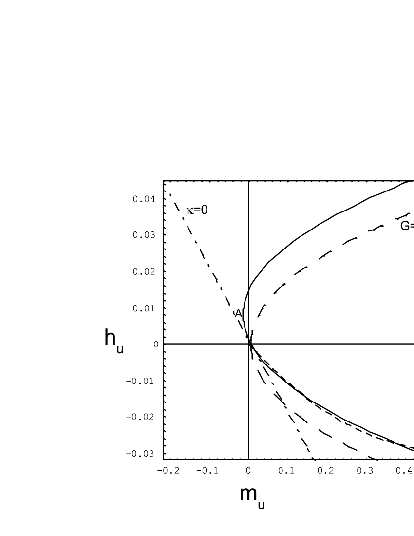
Figure 1: The function $h_{u}(m_{u})$ (here $[h_{u}]=\mbox{GeV}^{3}$, $[m_{u}]=\mbox{GeV})$ at fixed values $\hat{m}_{u}=6\ \mbox{MeV},\ \Lambda=860\ \mbox{MeV}$ for $G=0,\kappa=-5000\ \mbox{GeV}^{-5}$ (large dashes), $G=5\ \mbox{GeV}^{-2},\kappa=0$ (dash-dotted line), $G=5\ \mbox{GeV}^{-2},\kappa=-5000\ \mbox{GeV}^{-5}$ (solid line). The small-dashes line corresponds to the function $2\alpha_{u}(m_{u})$.

$2\pi^{2}\Delta_{i}=N_{c}Gm_{i}J_{0}(m_{i})$ for the theory without the ’t Hooft determinant. Alternatively one could consider the theory with only the ’t Hooft interaction (1) taking the limit $G\rightarrow 0$ in Eq.(3.1). In this case we obtain for $h_{u}^{(1)}$

$$h_{u}^{(1)}=\frac{4}{\kappa}\sqrt{-\kappa\Delta_{u}}=4\ \mbox{sign}(\kappa)\sqrt{\frac{\Delta_{u}}{-\kappa}}\quad(G=0).$$ (61)

In Fig.1 we plot three different stationary trajectories $h_{u}=h_{u}(m_{u})$ (with corresponding parameter values given in the caption) as functions of the quark mass $m_{u}$. To be definite we put the current quark mass equal $\hat{m}_{u}=6\ \mbox{MeV}$ and the cutoff parameter is choosen to be $\Lambda=860\ \mbox{MeV}$. By fixing $\Lambda$ we completely fix the curve corresponding to the right-hand side of the gap equation, i.e. the function $2\alpha_{u}=-N_{c}m_{u}J_{0}(m_{u}^{2})/(2\pi^{2})$. This function starts at the origin of the coordinate system, being always negative for positive values of $m_{u}$. At the point $m_{u}=\bar{m}\simeq 0.74\Lambda$ it has a minimum $\alpha_{u}^{(min)}=-\Lambda^{4}\bar{m}/[3(\Lambda^{2}+\bar{m}^{2})]$. All stationary trajectories cross the $m_{u}$-axis at the point $m_{u}=\hat{m}_{u}$. The straight line corresponds to the case $\kappa=0$. The second limiting case, $G=0$, is represented by the solution (61) and marked by $G=0$. The solid curve corresponds to Eq.(3.1), starts at the turning point $A$ with the coordinates $A(m_{u},h_{u})=(\hat{m}_{u}+4G^{2}/\kappa,-8G/\kappa)$ and goes monotonically down $(h_{u}^{(1)})$ and up $(h_{u}^{(2)})$ for increasing values of $m_{u}$. The standard assignment of signs for the couplings $G$ and $\kappa$: $G>0,\kappa<0$ is assumed. The points where $h_{u}(m_{u})$ intersects $2\alpha_{u}$ are the solutions of the gap equation. Let us remind Bernard:1988 that there are two qualitatively distinct classes of solutions. The first one is known as a solution with barely broken symmetry. We have this solution when $h_{u}$ intersects $2\alpha_{u}$ on the left side of its minimum (the minimum of $\alpha_{u}$ is outside the region shown in the figure). If $h_{u}$ crosses $2\alpha_{u}$ on the right side of its minimum it corresponds to the case with the firmly broken symmetry. It is known

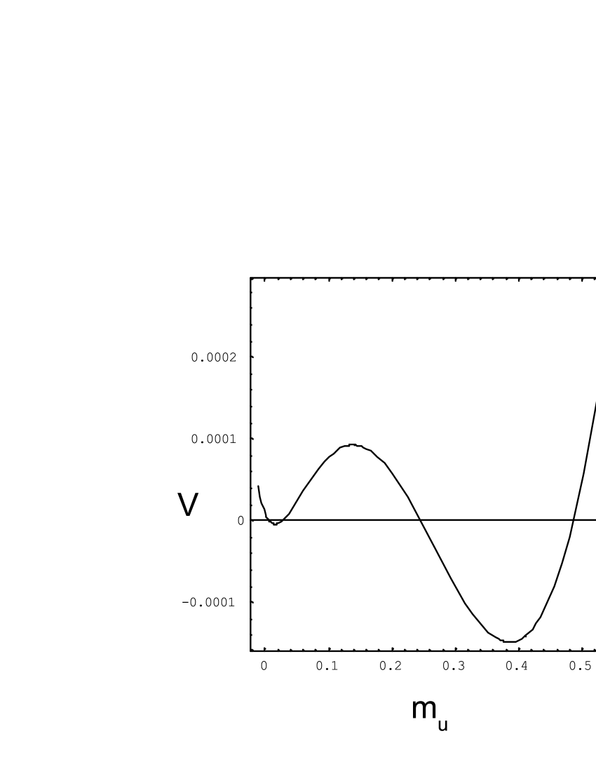
Figure 2: The $\hbar$ leading order effective potential $V(m_{u})$ corresponding to the pattern shown by the solid line on Fig.1. We use the units $[V]=[m_{u}]=\mbox{GeV}$.

that the theory responds quite differently to the introduction of a bare quark mass for these two cases. The barely broken regime is characterized by strong non-linearities reflected in the behaviour of expectation values of the scalar quark densities, $\bar{q}_{i}q_{i}$, in the physical quark states. Nevertheless, the solutions with the barely broken symmetry are likely to be more reliable from the physical point of view, in particular, when $\Lambda\simeq 0.5\ \mbox{GeV}$ and higher.

The six-quark interactions add several important new features into the picture. For instance, for some set of parameters, when $4G^{2}\sim\hat{m}_{u}|\kappa|$ or $G=0$, one can get three solutions of the gap equation, instead of one when $\kappa=0$. One of these cases is illustrated in Fig.1 for the parameter set $G=5\ \mbox{GeV}^{-2},\ \kappa=-5000\ \mbox{GeV}^{-5}$. The first solution is located quite close to the current quark mass value and, being a minimum of the effective potential, corresponds to the regime without the spontaneous breakdown of chiral symmetry. The next solution is a local maximum. The third one is a minimum and belongs to the regime with barely broken phase. The types of extrema are shown in Fig.2, where we used Eq.(78) with $\Omega^{-1}=0$ for the effective potential at leading order.

The second new feature is that the stationary trajectories $h_{u}(m_{u})$ in the case $\kappa\neq 0$ are real only starting from some value of $m_{u}\geq m_{min}$. For other values of $m_{u}$ where $m_{u}<m_{min}$ the effective energy is complex. To exclude this unphysical region the effective potential $V(m_{u})$ must be defined as a single-valued function on an half-open interval $m_{u}\geq m_{min}$.

3.2 NLO corrections: $z_{i}$ in the case of $SU(3)$ symmetry

The functions $z_{i}$ can be evaluated explicitly. To this end it is better to start from the case with $SU(3)$ flavor symmetry. This assumption involves a significant simplification in the structure of the semiclassical corrections, giving us however a result which possesses all the essential features of the more elaborate cases. Noticing that as a consequence of $SU(3)$ symmetry the function $h_{a}$ has only one non zero component $h_{0}$, one can find

$$A_{acb}h_{b}=A_{ac0}h_{0}=\frac{1}{3}\left(2\delta_{a0}\delta_{c0}-\delta_{a\alpha}\delta_{c\alpha}\right)h_{u}$$ (62)

where $\alpha=1,2\ldots 8.$ This result determines in general the structure of all flavor multi-indices objects like, for instance, $h_{ab}^{(1,2)}$ defined by the Eq.(2). Indeed, taking into account (62), one can represent algebraic equations for $h_{ab}^{(1,2)}$ in the form

$$G\left[\delta_{a0}\delta_{c0}\left(1\pm 2\omega\right)+\delta_{a\alpha}\delta_{c\alpha}\left(1\mp\omega\right)\right]h_{cb}^{(1,2)}=-\delta_{ab}\ ,$$

$$\omega=\frac{\kappa h_{u}}{16G}$$ (63)

where we follow the notation explained in Appendix A. Since this expression is a diagonal matrix, one can easily obtain

$$h_{cb}^{(1,2)}=-\frac{\delta_{c0}\delta_{b0}}{\displaystyle G\left(1\pm 2\omega\right)}-\frac{\delta_{c\alpha}\delta_{b\alpha}}{\displaystyle G\left(1\mp\omega\right)}\ ,$$ (64)

with $h_{cb}^{(1)}$ associated with the upper sign.

Consider now the perturbation term of Eq.(3). One can verify that

$$(h_{ab}^{(1)}-h_{ab}^{(2)})A_{abc}=\frac{\kappa h_{u}}{8G^{2}}\left(\frac{2A_{00c}}{1-4\omega^{2}}-\frac{\displaystyle\sum_{\alpha=1}^{8}A_{\alpha\alpha c}}{1-\omega^{2}}\right)$$ (65)

$$= \frac{\kappa h_{u}}{2G^{2}}\sqrt{\frac{2}{3}}\delta_{c0}\frac{1-3\omega^{2}}{(1-4\omega^{2})(1-\omega^{2})}\ .$$

Here we used the properties of the coefficients $A_{abc}$

$$A_{00c}=\frac{2}{3}\sqrt{\frac{2}{3}}\delta_{c0},\qquad A_{abb}\equiv\sum_{b=0}^{8}A_{abb}=-2\sqrt{\frac{2}{3}}\delta_{a0}.$$ (66)

The quantum effect of auxiliary fields to the gap equation stems from the term

$$(h_{ab}^{(1)}-h_{ab}^{(2)})A_{abc}h_{ci}^{(1)}=-\frac{\kappa h_{u}}{3G^{3}}\frac{1-3\omega^{2}}{(1+2\omega)(1-4\omega^{2})(1-\omega^{2})}$$ (67)

where the right-hand side is the same for the three possible choices of the index $i=u,d,s$. We conclude that in the $SU(3)$ limit the functions $z_{i}$ are uniquely determined by

$$z_{u}=-\frac{\kappa}{2G^{2}}\Omega^{-1}\frac{\omega(1-3\omega^{2})}{(1+2\omega)(1-4\omega^{2})(1-\omega^{2})}\ .$$ (68)

A direct application of (68) is the evaluation of the corrections $\Delta m_{i}$ to the constituent quark mass,

$$\Delta m_{u}=\frac{\kappa}{2G}\Omega^{-1}\frac{\omega(1-3\omega^{2})}{(1-4\omega^{2})(1-\omega^{2})}\ {\cal Q}_{u}\ .$$ (69)

This result is based on Eq.(139) and Appendix B. The right-hand side must be calculated with the leading order value of $m_{u}=M_{u}$. The factor ${\cal Q}_{u}$ is

$${\cal Q}_{u}=\frac{1}{1-(1+2\omega)I_{u}(m_{u}^{2})}\ .$$ (70)

Here the function $I_{i}(m_{i}^{2})$ is proportional to the derivative of the quark condensate $<\bar{q}_{i}q_{i}>$ with respect to $m_{i}$

$$I_{i}\equiv\frac{N_{c}G}{2\pi^{2}}\left[J_{0}(m_{i}^{2})-2m_{i}^{2}J_{1}(m_{i}^{2})\right],\qquad i=u,d,s$$ (71)

where the integral $J_{1}$ is given by

$$J_{1}(m^{2}) = -\frac{\partial}{\partial m^{2}}J_{0}(m^{2})=\int_{0}^{\infty}\frac{dt}{t}e^{-tm^{2}}\rho(t,\Lambda^{2})$$ (72)

$$= \ln\left(1+\frac{\Lambda^{2}}{m^{2}}\right)-\frac{\Lambda^{2}}{\Lambda^{2}+m^{2}}\ .$$

One can show that ${\cal Q}_{u}$ is related to the expectation values of the scalar quark density, $\bar{q}_{i}q_{i}$ in the physical quark state $|Q_{u}>$. To be precise we have ${\cal Q}_{u}={\cal Q}_{uu}+{\cal Q}_{ud}+{\cal Q}_{us}$, where the expectation values ${\cal Q}_{ui}$ are given in Appendix B. It is of interest to know the sign of the quasi-classical correction $\Delta m_{u}$. In general the answer on this question depends on the values of coupling constants which should be fixed from the hadron mass spectrum. All what we know at the moment is only that $G>0,\ \kappa<0,\ \hat{m}_{u}\simeq 6\ \mbox{MeV}$ and $\Lambda\sim 1\ \mbox{GeV}$. One can expect also that the dynamical masses of the quarks $M_{u}$ are close to their empirical value $M_{u}\simeq M_{N}/3\sim 300\ \mbox{MeV}$, with $M_{N}$ the nucleon mass. Let us suppose now that $0<\omega\ll 1$, what actually means that the coupling constants belong to the interval $0<-\kappa(M_{u}-\hat{m}_{u})/(4G)^{2}\ll 1$. This range is preferable from the point of view of $1/N_{c}$ counting. In this case we have

$$\Delta m_{u}\simeq\frac{\kappa\omega}{2G}\ \Omega^{-1}{\cal Q}_{u}^{\omega=0}$$ (73)

and one can conclude that the sign of $\Delta m_{u}$ is opposite to the sign of ${\cal Q}_{u}^{\omega=0}$. In turn the function ${\cal Q}_{u}^{\omega=0}$ is positive in some physically preferable range of values of $G$ such that $G\sim 5\ \mbox{GeV}^{-2}$.

It must be emphasized that the approximation made in Eq.(69) is legitimate only if the quasi-classical correction $\Delta m_{u}$ is small compared with the leading order result $M_{u}$. In particular, it is clearly inapplicable near points where the function ${\cal Q}_{u}(m_{u})$ has a pole. One sees from Eq.(70) that this takes place beyond some large values of $G$ or $\kappa$. There is a set of parameters for which the function $(1+2\omega)I_{u}(m_{u}^{2})$ is always less than $1$. This is the case, for instance, for the choice just considered above. For large couplings, ${\cal Q}_{u}$ may have a pole, and one has to check that the mean field result $M_{u}$ is located at a safe distance from them before using formula (69). The large couplings contain also the potential danger to meet the poles at the points $\omega=1$ and $\omega=1/2$. These poles are induced by caustics in the Gaussian path integral and occur as singularities in the effective potential.

We conclude this section with the expression for the quark condensate at next to leading order in $\hbar$,

$$<\bar{q}_{u}q_{u}>=<\bar{q}_{u}q_{u}>_{0}-\frac{\Delta m_{u}}{2G}I_{u}(M_{u}^{2}),$$ (74)

where the subscript $0$ denotes that the expectation value has been obtained in the mean field approximation.

3.3 NLO contribution to the effective potential: $SU(3)$ symmetric result

The expectation value of the energy density in a state for which the scalar field has the expectation value $\Delta_{i}$ is given by the effective potential $V(\Delta_{i})$. The effective potential is a direct way to study the ground state of the theory. If $V(\Delta_{i})$ has several local minima, it is only the absolute minimum that corresponds to the true vacuum. A sensible approximation method to calculate $V(\Delta_{i})$ is the semiclassical expansion Coleman:1988 . The first term in the expansion of $V$ is the classical potential. In the considered theory it contains the negative sum of all nonderivative terms in the bosonized Lagrange density which includes the one-loop quark diagrams and the leading order SPA result (30). The second term contains semiclassical corrections from Eq.(54) and the one-loop meson diagrams. However, one can obtain the effective potential directly from the gap equation. Indeed, let us assume that the potential $U(\sigma_{a},\phi_{a})$ of the Lagrange density of the bosonized theory is known, then $<U(\sigma_{a},\phi_{a})>=V(\Delta_{i})$. To explore the properties of the spontaneously broken theory, we restrict ourselves to the part of the total potential, $U(\sigma_{i})$, involving only the fields which develop a nonzero vacuum expectation value, $<\sigma_{i}>=\Delta_{i}$. Expanding $U(\sigma_{i})$ about the asymmetric ground state, we find

$$U(\sigma_{i})=U(\Delta_{i})+\left.\frac{\partial U}{\partial\sigma_{i}}\right|_{\sigma_{i}=\Delta_{i}}(\sigma_{i}-\Delta_{i})+\ldots\ .$$ (75)

It is clear that $U(\Delta_{i})=V(\Delta_{i})$, and the derivatives are functions of $\Delta_{j}$

$$\left.\frac{\partial U}{\partial\sigma_{i}}\right|_{\sigma_{i}=\Delta_{i}}=\left\langle\frac{\partial U}{\partial\sigma_{i}}\right\rangle=\frac{\partial V(\Delta_{j})}{\partial\Delta_{i}}=f_{i}(\Delta_{j}).$$ (76)

It means, in particular, that we can consider Eq.(76) as a system of linear differential equations to extract the effective potential $V(\Delta_{i})$, if the dependence $f_{i}(\Delta_{j})$ is known.

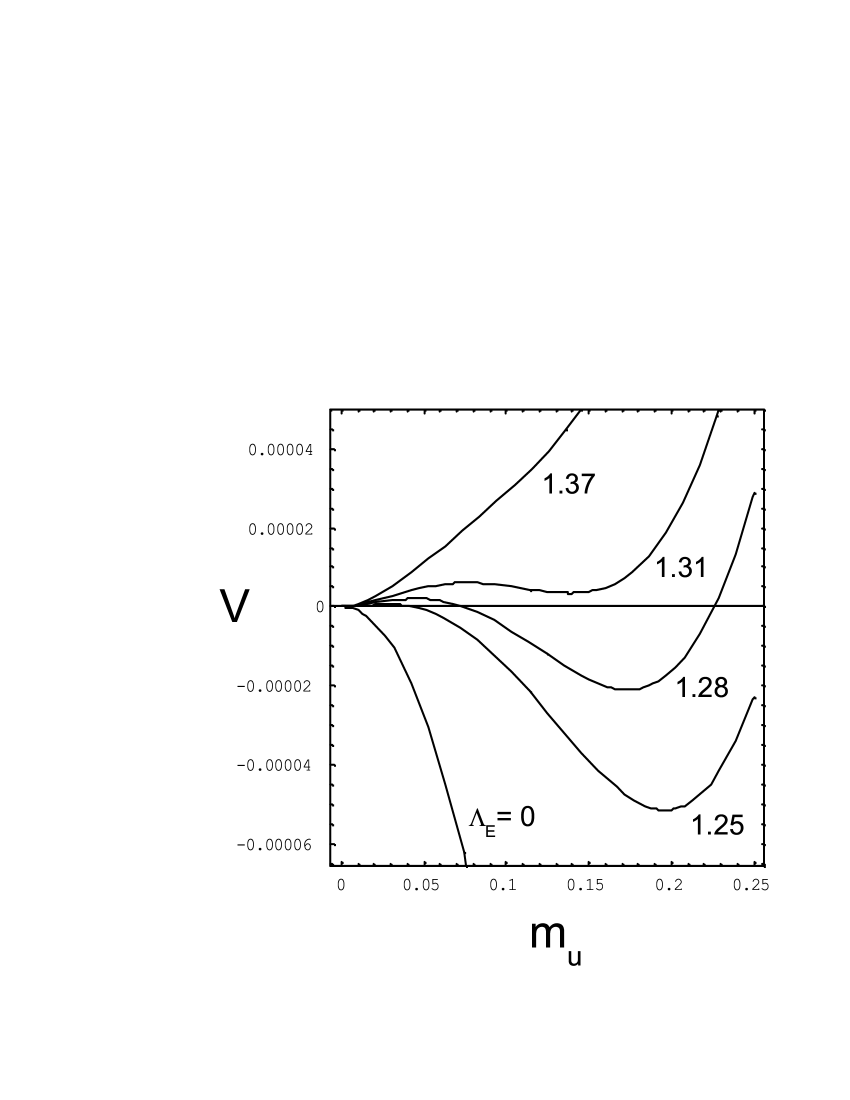
Figure 3: The effective potential $V(m_{u})$ to $\hbar$-order corresponding to the case $\kappa=-1800\ \mbox{GeV}^{-5}$, $G=10\ \mbox{GeV}^{-2}$, $\hat{m}=0$ and $\Lambda=860\ \mbox{MeV}$, where the values of $\Lambda_{E}$ are a measure for the strength of the NLO corrections in the effective potential. The units are $[V]=[m_{u}]=\mbox{GeV}$.

Further, Eq.(75) tells us that $f_{i}(\Delta_{j})$ are determined by the tadpole term in a shifted potential energy, $U(\sigma_{i}^{\prime}+\Delta_{i})$, where we define a new quantum field with vanishing vacuum expectation value $\sigma_{i}^{\prime}=\sigma_{i}-\Delta_{i}$. In the case of $SU(3)$ flavor symmetry, we have $f_{i}=f$ where $i=u,d,s$ and $f$ is given by

$$f(m_{u}) = -\frac{h_{u}}{2}-\frac{N_{c}}{4\pi^{2}}m_{u}J_{0}(m_{u}^{2})$$ (77)

$$- \frac{\kappa\Omega^{-1}\omega(1-3\omega^{2})}{4G^{2}(1+2\omega)(1-4\omega^{2})(1-\omega^{2})}\ .$$

Therefore, the condition for the extremum $\partial V(\Delta_{u})/\partial\Delta_{u}=0$ coincides with the gap equation (3). In Appendix C we obtain from Eq.(76) in the $SU(3)$ limit the effective potential

$$V(\Delta_{u}) = \frac{1}{4}\left(3Gh_{u}^{2}+\frac{\kappa}{4}h_{u}^{3}\right)-\frac{3}{2}v(m_{u}^{2})$$ (78)

$$- \frac{1}{2}\Omega^{-1}\ln\left|(1-4\omega^{2})(1-\omega^{2})^{8}\right|-C.$$

The free constant $C$ can be fixed by requiring $V(0)=0$. In this expression $v(m_{u}^{2})$ is defined according to Eq.(149) and $h_{u}$ is the first of the two solutions of the stationary point equation given by (3.1). Notice, that these solutions are complex when $4G^{2}<\kappa\Delta_{u}$. Hence the function $V(\Delta_{u})$ is not real as soon as the inequality is fulfilled. The most efficient way to go round this problem and to define the effective potential as a real function on the whole real axis is to treat $h_{u}$ as an independent variational parameter instead of $\Delta_{u}$ in Eq.(78). In this approach, which actually corresponds more closely to the BCS theory of superconductivity, one should consider equation (144) as the one which yields the function $\Delta_{u}(h_{u})$. One can check now that the extremum condition $\partial V(h_{u})/\partial h_{u}=0$ is equivalent to the gap equation (3) where the quark mass is expressed in terms of $h_{u}$ Hatsuda:1994 . Thus, the effective potential in the form of $V(h_{u})$ provides for a direct way to determine the minimum of the vacuum energy irrespectively of the not well defined mapping $\Delta_{u}\rightarrow h_{u}$.

There is a direct physical interpretation of Eq.(78): classically, the system sits in a minimum of the potential energy, $U_{cl}$, determined by the first two terms, and its energy is the value of the potential at the minimum, $U_{cl}(M_{u})$. To get the first quantum correction, $\Delta U$, to this picture, we add the third term $(\sim\Omega^{-1})$, and approximate the potential, $V(M_{u}+\Delta m_{u})$, near the classical minimum by a function $U_{cl}(M_{u})+\Delta U(M_{u})$.

In Fig.3 we show the effective potential calculated for $\kappa=-1800\ \mbox{GeV}^{-5},\ G=10\ \mbox{GeV}^{-2},\ \hat{m}=0$ and $\Lambda=860\ \mbox{MeV}$ depending on the strength of the fluctuations, indicated by the Euclidean cutoff $\Lambda_{E}$. In absence of fluctuations the minimum occurs at $m_{u}=M_{min}=340\ \mbox{MeV}$ (outside the range of this figure). Increasing the effect of fluctuations, the minima $M_{min}$ appear at smaller values and the potential gets shallower. Simultaneously a barrier develops between $V(0)$ and $V(M_{min})$. At some critical value of $\Lambda_{E}$ the point $V(0)$ becomes the stable minimum and the trivial vacuum is restored. This effect has a simple explanation. In the neighbourhood of the trivial vacuum where $m_{u}$ is small the effective potential $V(m_{u})$ can be well described by the first terms of the series in powers of $m_{u}$

$$\left.V(\Delta_{u})\right|_{\hat{m}=0} = \frac{3m_{u}^{2}}{4G}\left[1-\frac{N_{c}G\Lambda^{2}}{2\pi^{2}}+\frac{\kappa^{2}}{32G^{3}}\left(\frac{\Lambda_{E}}{2\pi}\right)^{4}\right]$$ (79)

$$+ {\cal O}(m_{u}^{3}).$$

The trivial vacuum always exists when

$$1-\frac{N_{c}G\Lambda^{2}}{2\pi^{2}}+\frac{\kappa^{2}}{32G^{3}}\left(\frac{\Lambda_{E}}{2\pi}\right)^{4}\geq 0.$$ (80)

This inequality generalizes the well-known result for $\kappa=0$.

The local minima $M_{min}$ in the broken phase are the exact solutions of the full gap equation (3). We find that at leading $\hbar$-order, $M_{min}^{pert}=M_{u}+\Delta m_{u}$, where $\Delta m_{u}$ is the correction (69), follows within a few percent the pattern shown for $M_{min}$ in Fig.3. For instance, one has at $\Lambda_{E}=1.25\ \mbox{GeV},\ M_{min}^{pert}=214\ \mbox{MeV}$, and at $\Lambda_{E}=1.31\ \mbox{GeV},\ M_{min}^{pert}=188\ \mbox{MeV}$. It is clear that the phase transition shown in Fig.3 is a non-perturbative effect. Instead the perturbative result yields $M_{min}^{pert}\rightarrow 0$ smoothly with increasing $\Lambda_{E}$ up to the value $\Lambda_{E}\simeq 1.6$ GeV.

Going to higher values of $m_{u}$ (not shown in Fig.3) one can come to caustics, i.e. singularities in $V(\Delta_{u})$. From the logarithm in Eq.(78) we obtain the values $\Delta_{u}$ where it happens. There are two singular points

$$\Delta_{u}^{(1)}=-12\frac{G^{2}}{\kappa}\ ,\qquad\Delta_{u}^{(2)}=-32\frac{G^{2}}{\kappa}\ .$$ (81)

For given values of couplings $G$ and $\kappa$ we have $\Delta_{u}^{(1)}=667\ \mbox{MeV}$ and $\Delta_{u}^{(2)}=1.78\ \mbox{GeV}$. The indicated curves with $\Lambda_{E}\neq 0$ have as asymptote the vertical line crossing the $m_{u}$-axis at the point $\Delta_{u}^{(1)}$. It is clear that for other parameter choices the ordering $\Delta_{u}^{(1)}<M_{u}<\Delta_{u}^{(2)}$, or even $\Delta_{u}^{(1)}<\Delta_{u}^{(2)}<M_{u}$ are possible, where $M_{u}$ is the classical minimum. In these cases a careful treatment of the caustic regions must be done.

3.4 Gap equation at leading order: $SU(2)_{I}\times U(1)_{Y}$ case, general properties

We will now apply the same strategy to the case $\hat{m}_{u}=\hat{m}_{d}\neq\hat{m}_{s}$, which breaks the unitary $SU(3)$ symmetry down to the $SU(2)_{I}\times U(1)_{Y}$ (isospin-hypercharge) subgroup. In full agreement with symmetry requirements it follows then that $m_{u}=m_{d}\neq m_{s}$ and $h_{u}=h_{d}\neq h_{s}$. Thus, we have a system of two equations (from Eq.(31)) to determine the functions $h_{u}$ and $h_{s}$. These equations can be easily solved in the limit $G\rightarrow 0$

$$h_{u}=-4\sqrt{\frac{\Delta_{s}}{-\kappa}}\ \ ,\qquad h_{s}=\frac{4}{\kappa}\Delta_{u}\sqrt{\frac{-\kappa}{\Delta_{s}}}\quad(G=0).$$ (82)

Obviously the result Eq.(61) follows from these expressions. For $G\neq 0$ the system is equivalent to the following one

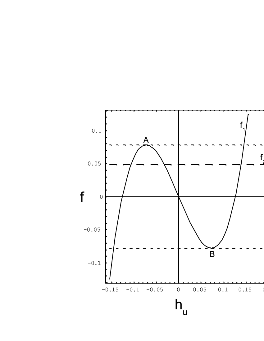
Figure 4: Graphical solution of the cubic equation in (83). The left-hand $(f_{1})$ and the right-hand $(f_{2})$ sides of this equation are plotted as a function of $h_{u}$ for $x_{s}<1$. The region bounded by the dashed lines corresponds to the interval $D<0$ where the cubic equation has three real solutions. The local maximum $A$ and the local minimum $B$ have coordinates $A:\{h_{u}=-\sqrt{-Q},\ f=\Delta(x_{s})/G\}$ and $B:\{h_{u}=\sqrt{-Q},\ f=-\Delta(x_{s})/G\}$.

$$\left\{\begin{array}[]{rcl}\displaystyle\left(\frac{\kappa}{16G}\right)^{2}h_{u}^{3}+(x_{s}-1)h_{u}&=&\displaystyle\frac{\Delta_{u}}{G}\\ &&\\ Gh_{s}+\Delta_{s}+\displaystyle\frac{\kappa}{16}h_{u}^{2}&=&0\\ \end{array}\right.$$ (83)

where we put $x_{s}=\kappa\Delta_{s}/(4G)^{2}$ in accordance with our notation in the Appendix A. From the physics of instantons we know that the strength constant $\kappa<0$. It makes $x_{s}$ negative. Hence the left-hand side of the first equation is not a monotonic function of $h_{u}$ (see Fig.4). The right-hand side is a positive constant, if $\Delta_{u}>0$ and $G>0$, what is usually assumed. Therefore, the equation has three different real solutions, $h_{u}^{(n)}(\Delta_{u},\Delta_{s}),\ n=1,2,3$, in some interval of values for $\Delta_{u}/G$. The boundaries of the interval are given by the inequality $-\Delta(x_{s})<\Delta_{u}<\Delta(x_{s})$, where

$$\Delta(x_{s})=\frac{32G^{2}}{|\kappa|}\left(\frac{1-x_{s}}{3}\right)^{3/2}_{.}$$ (84)

By means of the discriminant $D$ of the cubic equation, $D=Q^{3}+R^{2}$, where

$$Q=\left(\frac{16G}{\kappa}\right)^{2}\frac{x_{s}-1}{3}\ ,\qquad R=\left(\frac{16G}{\kappa}\right)^{3}\frac{x_{u}}{2}\ ,$$ (85)

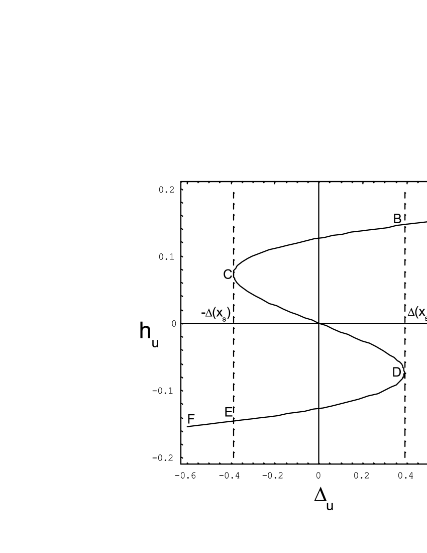
Figure 5: The stationary trajectory $h_{u}(\Delta_{u})$ at fixed $\Delta_{s}$. Inside the interval $|\Delta_{u}|<\Delta(x_{s})$ it is a multi-valued mapping. The monotonic curves: $BC,CD,DE$ correspond to the three well-defined single-valued functions: $h_{u}^{(n)},n=1,2,3.$

this region can be shortly identified by $D<0$. The qualitative picture of the dependence $h_{u}(\Delta_{u})$ at a fixed value of $\Delta_{s}$ is shown in Fig.5. The three solutions in the region $D\leq 0$ can be parametrized by the angle $\varphi$

$$h_{u}^{(1)} = 2\sqrt{-Q}\cos\frac{\varphi}{3}\ ,\quad h_{u}^{(2)}=2\sqrt{-Q}\sin\left(\frac{\varphi}{3}-\frac{\pi}{6}\right),$$

$$h_{u}^{(3)} = -2\sqrt{-Q}\sin\left(\frac{\varphi}{3}+\frac{\pi}{6}\right)$$ (86)

where

$$\cos\varphi=\frac{R}{\sqrt{-Q^{3}}}\ ,\quad\sin\varphi=\sqrt{1+\frac{R^{2}}{Q^{3}}}\ .$$ (87)

The angle $\varphi$ can always be converted to values of $\varphi$ such that $0\leq\varphi\leq\pi$. The boundaries $\varphi=0$ and $\varphi=\pi$ correspond to the value $D=0$. When the argument $\varphi$ increases from $0$ to $\pi$, the solutions $h_{u}^{(1)},h_{u}^{(2)}$ and $h_{u}^{(3)}$ run along the curves $BC,DC$ and $DE$ accordingly. These curves intersect the $h_{u}$-axis at $\varphi=\pi/2$, where $R=0$. One can show that $h_{u}^{(2)}\rightarrow-\Delta_{u}/G$ at $\kappa\rightarrow 0$ in full agreement with our previous result following from Eq.(3.1). On the other side $h_{u}^{(3)}$ leads to the result (82) in the limit $G\rightarrow 0$. Previously, studying the $SU(3)$ case, we have obtained both of these limits from one solution (3.1). Now one has to use either solution $h_{u}^{(2)}$ or solution $h_{u}^{(3)}$ depending on the values of the parameters $\kappa,G,\Delta_{u}$, and $\Delta_{s}$ which correspond to the minimum of the energy density. There is no chance to join the partial cases $G=0$ and $\kappa=0$ in one solution, because they lead to systems of quadratic (in the first case) and linear (in the second case) equations without intersection of their roots. The stationary trajectory $h_{u}^{(1)}$ is a positive definite function and thus the solution of the gap equation does not belong to this branch.

Let us suppouse that the system of two equations which describe the vacuum state of the theory in the case of the $SU(2)_{I}\times U(1)_{Y}$ symmetry at leading order has a solution, i.e., the constituent quark masses $M_{u(1)}$ and $M_{s(1)}$, corresponding to a local extremum of the effective potential $V(m_{u},m_{s})$, are known. We may assume that $M_{u(1)}$ belongs to the region with the barely broken symmetry, $M_{u(1)}<\bar{m}_{u}$. As we already know, it is the most preferable pattern from the physical point of view. Then there is no any other solution $M_{u(1)}^{\prime}\neq M_{u(1)}$ for this set of parameters $G,\kappa,\Lambda,\hat{m}_{u},\hat{m}_{s}$ and already fixed value $M_{s(1)}$. This follows from the pure geometrical fact that the second order derivatives for curves $h_{u}(\Delta_{u})$ and $<\bar{q}_{u}q_{u}>$ have opposite signs in the considered region. Suppose further that there are other solutions $M_{u(n)},\ M_{s(n)}$ with $n=2,3.$ This statement does not contradict our previous result corresponding to the case with the $SU(3)$ symmetry, where we were able to find out three solutions for some sets of parameters. The functions $M_{u(n)}$ and $M_{s(n)}$ can be understood as chiral expansions about the $SU(3)$ symmetric solutions. The coefficients of the chiral series are determined by the expectation values ${\cal Q}_{ij}(M_{u})$ and their derivatives. It means that solutions in the case of $SU(3)$ symmetry are related to the solutions for the more general $SU(2)_{I}\times U(1)_{Y}$ case. Hence, there are only three sets of solutions $(M_{u(n)},M_{s(n)})$ at maximum (for the considered region). The effective potential helps us to classify these critical points as will be discussed in Sec. 3.6.

3.5 NLO corrections: $z_{i}$ and $\Delta m_{i}$ in the case of $SU(2)_{I}\times U(1)_{Y}$ symmetry

Our next task is to take into account quantum fluctuations and compute the corresponding corrections to the leading order result $M_{u},M_{s}$. For this purpose we need to find $z_{u}$ and $z_{s}$. Consider first the sum $A_{acb}h_{b}$ which can be written as a $9\times 9$ matrix in block diagonal form

$$A_{acb}h_{b}=-\frac{1}{3}\left(\begin{array}[]{ccc}\Omega_{1}&0&0\\ 0&\Omega_{2}&0\\ 0&0&\Omega_{3}\end{array}\right)$$ (88)

with $2\times 2$, $3\times 3$ and $4\times 4$ blocks

$$(\Omega_{1})_{rs} = \frac{1}{3}\left(\begin{array}[]{cc}-2(2h_{u}+h_{s})&\sqrt{2}(h_{u}-h_{s})\\ \sqrt{2}(h_{u}-h_{s})&(4h_{u}-h_{s})\end{array}\right)_{rs}\ ,$$ (91)

$$(\Omega_{2})_{nm} = h_{s}\delta_{nm}\ ,\quad(\Omega_{3})_{fg}=h_{u}\delta_{fg}\ .$$ (92)

The indicies $r,s$ of the first matrix range over the subset $r,s=0,8$ of the set $a,c=0,1,\ldots 8$. In the matrix $\Omega_{2}$ we assume that $n,m=1,2,3$ and in $\Omega_{3}$ the indices take values $f,g=4,5,6,7$.

Using this result one can solve the last two equations in (2), rewriting them in the form

$$G\left(\begin{array}[]{ccc}1\mp\displaystyle\frac{\kappa\Omega_{1}}{16G}&0&0\\ 0&1\mp\displaystyle\frac{\kappa\Omega_{2}}{16G}&0\\ 0&0&1\mp\displaystyle\frac{\kappa\Omega_{3}}{16G}\end{array}\right)_{ac}\!\!h_{ce}^{(1,2)}=-\delta_{ae}$$ (93)

and find the functions $h_{ce}^{(1,2)}$. We obtain

$$h_{nm}^{(1,2)}=\frac{-\delta_{nm}}{G(1\mp\omega_{s})}\ ,\qquad h_{fg}^{(1,2)}=\frac{-\delta_{fg}}{G(1\mp\omega_{u})}\ ,$$ (94)

where $\omega_{i}$ are defined in the Appendix A. For the $2\times 2$ matrix with indices $0,8$ we have

$$h^{(1,2)}_{rs} = \frac{-1}{3G(1\pm\omega_{s}-2\omega_{u}^{2})}$$ (98)

$$\left(\begin{array}[]{cc}3\mp(4\omega_{u}-\omega_{s})&\ \pm\sqrt{2}(\omega_{u}-\omega_{s})\\ \\ \pm\sqrt{2}(\omega_{u}-\omega_{s})&\ 3\pm 2(2\omega_{u}+\omega_{s})\end{array}\right)_{rs}.$$

In particular, if the terms $\omega_{u}$ and $\omega_{s}$ are equal, these expressions coincide with Eq.(64).

We now calculate the sum $A_{abc}h_{ab}$, where $h_{ab}\equiv h_{ab}^{(1)}-h_{ab}^{(2)}$. Using the properties of coefficients $A_{abc}$ and solutions for $h_{ab}^{(1,2)}$ obtained above, one can find that

$$A_{abc}h_{ab} = -\frac{1}{3}\sqrt{\frac{2}{3}}(h_{88}-2h_{00}+3h_{11}+4h_{44})\delta_{c0}$$ (99)

$$- \frac{2}{3\sqrt{3}}(h_{88}+\sqrt{2}h_{08}-3h_{11}+2h_{44})\delta_{c8}$$

$$\equiv H_{1}\delta_{c0}+H_{2}\delta_{c8}.$$

Again, from this equation the related formula (65) can be established by equating $\omega_{u}=\omega_{s}$. In this special case we have $H_{2}=0$. As a next step let us contract the result with functions $h_{ci}^{(1)}$

$$A_{abc}h_{ab}h_{ci}^{(1)}=\frac{1}{\sqrt{3}}$$ (100)

$$\left\{\begin{array}[]{ll}H_{1}(\sqrt{2}h^{(1)}_{00}+h^{(1)}_{08})+H_{2}(\sqrt{2}h^{(1)}_{08}+h^{(1)}_{88}),&i=u,d\\ \\ H_{1}(\sqrt{2}h^{(1)}_{00}-2h^{(1)}_{08})+H_{2}(\sqrt{2}h^{(1)}_{08}-2h^{(1)}_{88}),&i=s\end{array}\right.$$ (104)

These contributions can be evaluated explicitly. It leads to the final expressions for the semiclassical corrections $z_{i}$ to the gap equation (3). They are given by

$$\begin{array}[]{l}\displaystyle z_{u}=z_{d}\\ \\ \displaystyle=-\frac{\kappa\Omega^{-1}\omega_{u}}{8G^{2}\mu}\left[\frac{2(1-2\omega_{u}^{2})-\omega_{s}}{(1-2\omega^{2}_{u})^{2}-\omega_{s}^{2}}+\frac{2}{1-\omega_{u}^{2}}-\frac{3\omega_{s}}{1-\omega_{s}^{2}}\right],\\ \\ \displaystyle z_{s}=-\frac{\kappa\Omega^{-1}}{8G^{2}\mu}\left[\frac{4\omega^{2}_{u}(3\omega^{2}_{u}-2)+1+\omega_{s}}{(1-2\omega^{2}_{u})^{2}-\omega_{s}^{2}}+\frac{3}{1-\omega_{s}}\right.\\ \\ \displaystyle\left.\ \ \ \ \ \ \ \ \ \ \ \ \ \ \ \ \ \ \ \ -\frac{4}{1-\omega^{2}_{u}}\right],\end{array}$$ (105)

where $\mu=(1+\omega_{s}-2\omega_{u}^{2})$. Each of these formulas has the same limiting value at $\omega_{s}=\omega_{u}=\omega$ which coincides with Eq.(67).

We apply this result to establish the $\hbar$-order correction to the masses of constituent quarks. To this end we must use the general expressions obtained in Appendices A and B, which for the considered case we rewrite in a way that stresses the quark content of the contributions

$$\Delta m_{i}=-G\sum_{j,k=1}^{2}z_{j}{\cal M}_{jk}{\cal Q}_{(i)k}$$ (106)

where $i=u,s$, the $\hbar$-corrections $z_{j}$ are written as a line matrix $z_{j}=(z_{u},z_{s})$, and obviously $\Delta m_{u}=\Delta m_{d}$. The $2\times 2$ matrix ${\cal M}_{jk}$ and the column ${\cal Q}_{(i)k}$ are defined as follows

$${\cal M}_{jk}=\left(\begin{array}[]{cc}1+\omega_{s}&2\omega\\ \omega&1\end{array}\right),\qquad{\cal Q}_{(i)k}=\left(\begin{array}[]{c}{\cal Q}_{iu}+{\cal Q}_{id}\\ {\cal Q}_{is}\end{array}\right)_{k}.$$ (107)

Observe that $\mbox{det}{\cal M}=\mu$. The $\hbar$-corrections to the quark masses must be calculated at the point $(M_{u},\ M_{s})$, being a solution of the gap equation at leading order. The expression (69) is a straightforward consequence of the more general result (106). Let us also note that formula (106) clearly shows which part of the correction is determined by the strange component of the quark sea and which one by the non-strange contributions.

3.6 Effective potential: the $SU(2)_{I}\times U(1)_{Y}$ symmetry

We can now generalize the result obtained in the Sec. 3.3 to the case of $SU(2)_{I}\times U(1)_{Y}$ symmetry. To find the effective potential for this case one has to evaluate the line integral of the form

$$\int_{\gamma}2f_{u}dm_{u}+f_{s}dm_{s}=V(\Delta_{u},\Delta_{s})$$ (108)

where the independent variables $m_{u}$ and $m_{s}$ are linear combinations of the $SU(3)$ singlet and octet components $m_{u}=(\sqrt{2}m_{0}+m_{8})/\sqrt{3},\quad m_{s}=(\sqrt{2}m_{0}-2m_{8})/\sqrt{3}$. We also know that

$$f_{u}(m_{u},m_{s}) = -\frac{h_{u}}{2}-\frac{N_{c}}{4\pi^{2}}m_{u}J_{0}(m_{u}^{2})+\frac{z_{u}}{2}\ ,$$

$$f_{s}(m_{u},m_{s}) = -\frac{h_{s}}{2}-\frac{N_{c}}{4\pi^{2}}m_{s}J_{0}(m_{s}^{2})+\frac{z_{s}}{2}\ .$$ (109)

The functions $f_{u},f_{s}$ lie on the surface $S(m_{u},m_{s})$ defined by the stationary point equation (83), and $\gamma$ is contained in $S$. There are some troubles caused by the singularities in $z_{u},z_{s}$. The poles are located on curves which divide the surface $S(m_{u},m_{s})$ on distinct parts $\Sigma_{n}$. The integral (108) is well defined inside each of these regions $\Sigma_{n}$. It is characterized by the property that the integral over an arc $\gamma$, which is contained in $\Sigma_{n}$, depends only on its end points, i.e., the integral over any closed curve $\gamma_{c}$ contained in $\Sigma_{n}$ is zero. This follows from the fact that the integrand is an exact differential. Indeed, one can simply check that the one-form $2f_{u}dm_{u}+f_{s}dm_{s}$ is closed on $\Sigma_{n}$:

$$2\frac{\partial f_{u}}{\partial m_{s}}-\frac{\partial f_{s}}{\partial m_{u}}=0.$$ (110)

On the other hand, the open set $\Sigma_{n}$ is diffeomorphic to ${\bf R}^{2}$ and, by Poincaré’s lemma, the one-form is exact.

Direct verification is relatively cumbersome and can be done along the lines of our calculation in the Appendix C, as follows. Since each of the differentials $2h_{u}dm_{u}+h_{s}dm_{s}$ and $2z_{u}dm_{u}+z_{s}dm_{s}$ is closed, let us consider them separately. We begin by evaluating the first one-form

$$-(2h_{u}dm_{u}+h_{s}dm_{s})=d\left(Gh_{u}^{2}+\frac{G}{2}h_{s}^{2}+\frac{\kappa}{8}h_{u}^{2}h_{s}\right)$$ (111)

where we have used Eqs.(31) to extract $dm_{u}$ and $dm_{s}$.

Noting that $3\kappa^{2}(h_{u}^{2}+Q)=-\mu(16G)^{2}$, one can obtain for the second one-form

$$2z_{u}dm_{u}+z_{s}dm_{s}=\frac{3\kappa}{16}\left(z_{s}+2\omega_{u}z_{u}\right)dQ-2G\mu z_{u}dh_{u}.$$ (112)

Let us note also that

$$z_{s}+2\omega_{u}z_{u}=-\frac{\kappa\Omega^{-1}\omega_{s}}{8G^{2}}\left[\frac{1}{(1-2\omega^{2}_{u})^{2}-\omega_{s}^{2}}+\frac{3}{1-\omega_{s}^{2}}\right].$$ (113)

Putting this expression in Eq.(112), we have after some algebra

$$2z_{u}dm_{u}+z_{s}dm_{s}$$

$$= \Omega^{-1}\left[\frac{\displaystyle d\omega_{s}^{2}+4(1-2\omega_{u}^{2})d\omega_{u}^{2}}{(1-2\omega_{u}^{2})^{2}-\omega^{2}_{s}}+\frac{3d\omega^{2}_{s}}{1-\omega_{s}^{2}}+\frac{4d\omega_{u}^{2}}{1-\omega_{u}^{2}}\right]$$

$$= -\Omega^{-1}d\ln\left|[(1-2\omega_{u}^{2})^{2}-\omega_{s}^{2}](1-\omega_{s}^{2})^{3}(1-\omega^{2}_{u})^{4}\right|.$$

Finally, we obtain the effective potential

$$\begin{array}[]{l}\displaystyle V(\Delta_{u},\Delta_{s})=\frac{1}{2}\left(Gh_{u}^{2}+\frac{G}{2}h_{s}^{2}+\frac{\kappa}{8}h_{u}^{2}h_{s}\right)\\ \displaystyle\ \ \ \ \ \ \ \ \ \ \ \ \ \ \ -v(m_{u}^{2})-\frac{1}{2}v(m_{s}^{2})-C\\ \displaystyle-\frac{\Omega^{-1}}{2}\ln\left|[(1-2\omega_{u}^{2})^{2}-\omega_{s}^{2}](1-\omega_{s}^{2})^{3}(1-\omega^{2}_{u})^{4}\right|\end{array}$$ (115)

where $v(m_{i}^{2})$ has been introduced in Eq.(149). The constant $C$ depends on the initial point of the curve $\gamma$, and in the region $\Sigma$ which includes the point $\Delta_{u}=0,\Delta_{s}=0$ it can be fixed by requiring $V(0,0)=0$. This result coincides with Eq.(78) in the $SU(3)$ limiting case.

In Fig.6 we show the effective potential calculated as function of condensates without the fluctuations, $\Omega^{-1}=0$, for the parameter set given in the caption. There are altogether nine critical points: four minima, four saddles and one maximum. Only one critical point is localized in the region of physical interest, the minimum for $m_{u},m_{s}>0$ (or $h_{u},h_{s}<0$). In the chiral limit and otherwise the same parameters one has three critical points of interest, the maximum at the origin, the saddle at $m_{u}=0,m_{s}>0$ ($h_{u}=0,h_{s}<0$), and the minimum. This distribution and behavior of critical points is common to a large set of parameters.

The behavior of $V(\Delta_{u},\Delta_{s})$ in terms of the strength of the fluctuation term $\sim\Omega^{-1}$ is qualitatively the same as for the $SU(3)$ case: fluctuations tend to restore the trivial vacuum in the region prior to the singularities. We also see from Eq.(115) that now the picture of singularities is more elaborated. Nevertheless attractive wells still develop between them.

These results are in agreement with the following topological consideration. The effective potential $V$ is a smooth function defined on the space of paths $S(h_{u},h_{s})$ diffeomorphic to ${\bf R}^{2}$ (before the onset of caustics). The Euler characteristic of the surface $S$, $\chi(S)=1$, can be expressed, by Morse’s theorem, through the number of non-degenerate critical points of the function $V$

$$\chi(S)=C_{0}-C_{1}+C_{2}$$ (116)

where $C_{0}$ is a number of critical points with index $0$ (minima), $C_{1}$ is a number of critical points with index $1$ (saddle-points), and $C_{2}$ is a number of critical points with index $2$ (maxima).

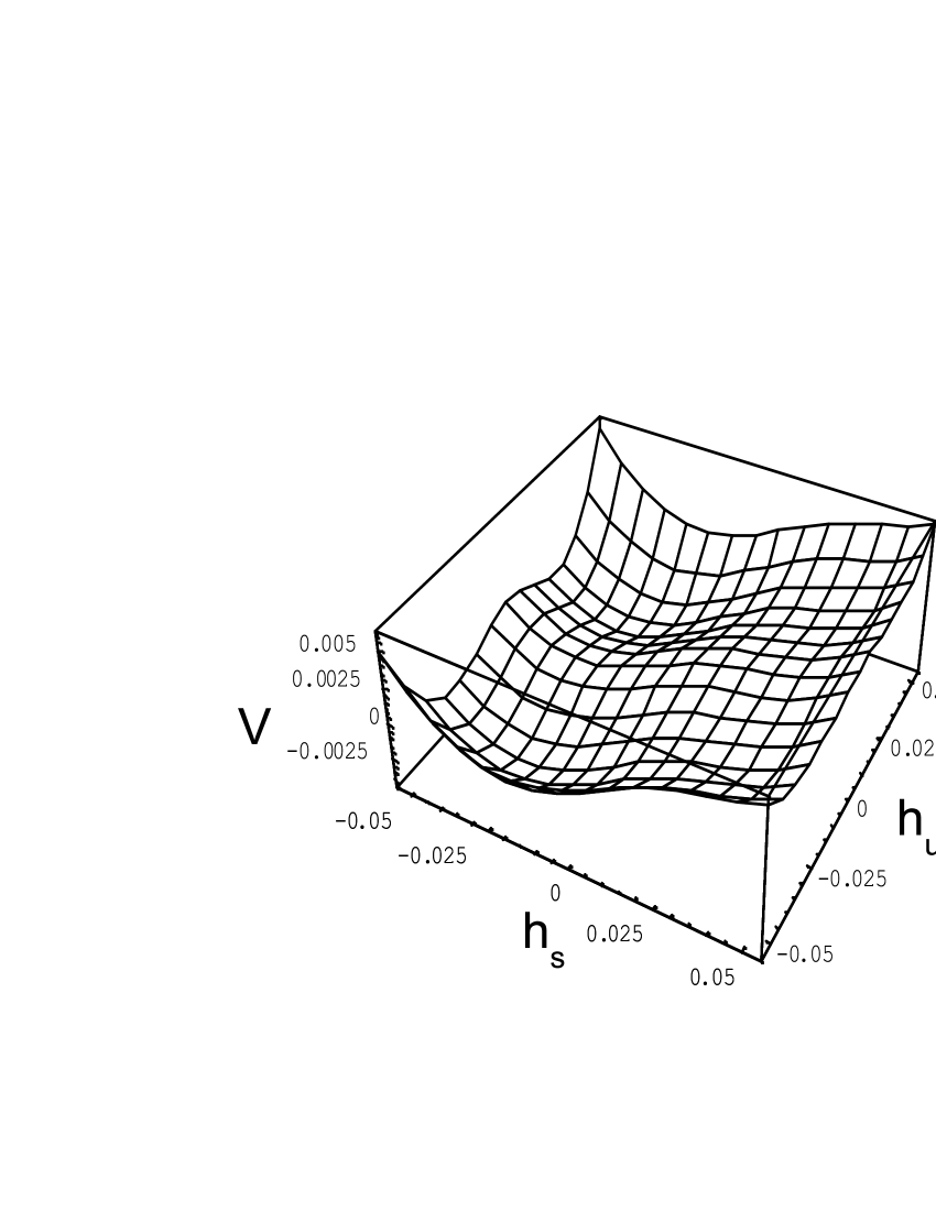
Figure 6: Classical effective potential $V[\mbox{GeV}]$, Eq.(115) with $\Omega^{-1}=0$, as function of condensates $[\mbox{GeV}^{-3}]$ $h_{u}=2<\bar{u}u>$, $h_{s}=2<\bar{s}s>$ for $\Lambda=860$ MeV, $G=14\ \mbox{GeV}^{-2},\ \kappa=-1000\ \mbox{GeV}^{-5},\ \hat{m}_{u}=6\ \mbox{MeV},\hat{m}_{s}=150\ \mbox{MeV}$.

4 The ground state in the $1/N_{c}$ expansion

We have considered till now the semiclassical approach to estimate the integral ${\cal Z}[\sigma,\phi;\Delta]$ in Eq.(19). However, rather than using $\hbar$ as the parameter of asymptotic expansion, we could also have used $1/N_{c}$ to estimate it. In this case the stationary phase equations (21) involve terms with different orders of $1/N_{c}$ and must be solved perturbatively. For this purpose let us represent (21) in a complex form

$$GU_{a}+W_{a}+\frac{3\kappa}{32}A_{abc}U^{\dagger}_{b}U^{\dagger}_{c}=0.$$ (117)

Indeed the first two terms are of order $(1/N_{c})^{0}$, since $G\sim 1/N_{c}$, $U\sim N_{c}$, and $W\sim N_{c}^{0}$, while the last one is of order $1/N_{c}$. Casting the solutions $U_{\mbox{st}}^{a}$ as a series in $1/N_{c}$ up to and including the terms of order $1/N_{c}$, we have

$$U^{a}_{\mbox{st}}=-\frac{1}{G}\left(W_{a}+\frac{3\kappa}{32G^{2}}A_{abc}W^{\dagger}_{b}W^{\dagger}_{c}+{\cal O}(1/N_{c}^{2})\right).$$ (118)

It yields for ${\cal L}_{r}(r_{\mbox{st}})$

$${\cal L}_{r}(r_{\mbox{st}}) = -\frac{1}{4G}\mbox{tr}(WW^{\dagger})-\frac{\kappa}{(4G)^{3}}\left(\det W+\det W^{\dagger}\right)$$ (119)

$$+ {\cal O}(1/N_{c}).$$

The contribution from the auxiliary fields can be obtained directly from Eq.(55) by expanding our solutions $h_{ab}$ and $h_{c}$ in a series in $1/N_{c}$. One can already conclude from that expression, without any calculations, that the term $\sim\Omega^{-1}$ is at most of order $\sim 1/N_{c}$. Therefore it is beyond the accuracy of the considered approximation and can be neglected. Actually, it follows from Eq.(2), that the difference $h_{ab}=h_{ab}^{(1)}-h_{ab}^{(2)}$ has order $\sim N_{c}^{0}$, additionally suppressing this contribution, i.e. for the correction to the result (119) we have only a term starting from $1/N_{c}^{2}$-order

$$\Delta{\cal L}_{r} = -\frac{\kappa^{2}\Omega^{-1}}{8(2G)^{4}}\left[\mbox{tr}(WW^{\dagger})+\frac{3\kappa}{(4G)^{2}}\left(\det W+\det W^{\dagger}\right)\right]$$ (120)

$$+ {\cal O}(1/N_{c}^{3}).$$

It means, in particular, that one can neglect this type of quantum fluctuations in the discussion of the gap equation up to and including the terms of $1/N_{c}$ order in the meson Lagrangian. These corrections cannot influence significantly the dynamical symmetry breaking phenomena in the model and only the quantum effect of mesons (the one-loop contributions of $\sigma$ and $\phi$ fields) together with the leading order contribution from the ’t Hooft determinant (see Eq.(119)) are relevant at $N_{c}^{0}$-order here.

If the model allows us to utilize the $1/N_{c}$ expansion, the vacuum state is defined by the gap equation obtained from Eq.(3) in the large $N_{c}$ limit, or, equivalently, on the basis of Lagrangian (119). We have

$$\Delta_{i}+\frac{\kappa}{32G^{2}}t_{ijk}\Delta_{j}\Delta_{k}=\frac{N_{c}G}{2\pi^{2}}m_{i}J_{0}(m_{i}).$$ (121)

At leading order in an $1/N_{c}$ expansion we have the standard gap equation $2\pi^{2}\Delta_{i}=N_{c}Gm_{i}J_{0}(m_{i})$. The terms arising on the next step already include the quantum correction from the ’t Hooft determinant. It is not difficult to obtain the corresponding contribution of order $1/N_{c}$ to the mass of constituent quarks

$$m_{i}=M_{i}+\Delta m_{i}\ ,$$

$$\Delta m_{i}=-\frac{\kappa\Delta_{j}\Delta_{k}}{(4G)^{2}(1-I_{i})}\qquad(i\neq j\neq k)$$ (122)

where $\Delta m_{i}$ is calculated at the point $m_{i}=M_{i}$, which is the solution of the gap equation (121) at leading order, and $I_{i}$ is given by Eq.(71). One can show that $\Delta m_{i}>0$, thus increasing the effect of the dynamical chiral symmetry breaking. This is an immediate consequence of the formula

$$1-I_{i}(M_{i}^{2})=\frac{\hat{m}_{i}}{M_{i}}+\frac{N_{c}G}{\pi^{2}}M_{i}^{2}J_{1}(M_{i}^{2})>0.$$ (123)

Let us stress that the first equality is fulfilled only at the point $M_{i}$.

We did not clarify yet the counting rule for the current quark masses $\hat{m}_{i}$, assuming that they are counted as the constituent quark masses. Actually, these masses are small and following the standard rules of ChPT one should consider $\hat{m}_{i}\sim 1/N_{c}$. In this case in the large $N_{c}$ limit the model possesses the $U(3)\times U(3)$ symmetry and the gap equation at leading order, $2\pi^{2}=N_{c}GJ_{0}(m_{i})$, leads to a solution with equal masses $M_{u}=M_{d}=M_{s}\equiv M$. The $1/N_{c}$ correction includes the $\kappa$-dependent term and the term depending on the current quark masses

$$\Delta m_{i}=\frac{\pi^{2}}{N_{c}G}\left(\hat{m}_{i}-\frac{\kappa M^{2}}{16G^{2}}\right)\frac{1}{M^{2}J_{1}(M^{2})}\ .$$ (124)

Returning back to Eq.(119) one can conclude that the large-$N_{c}$ limit corresponds to the picture which is not affected by six-quark fluctuations. This can be realized also directly from Lagrangian (30). Indeed, the couplings of meson vertices are determined here through the functions $h_{a}$ given in the case of $SU(3)$ flavor symmetry by $h_{u}^{(1)}$ in Eq.(3.1). The large-$N_{c}$ limit forces a series expansion for $h_{u}^{(1)}$ with a small parameter

$$\epsilon=\frac{|\kappa|\Delta_{u}}{4G^{2}}\sim\frac{1}{N_{c}}\ll 1$$ (125)

and the leading term $h_{u}^{(1)}=-\Delta_{u}/G+\ldots$ which does not depend on $\kappa$.

This observation leads us to the second important conclusion. It is easy to see that the parameter $\epsilon$ is an internal model parameter and the series expansion in $\epsilon$ closely corresponds to the $1/N_{c}$ expansion of the model. The existence of this small parameter allows us to consider the $1/N_{c}$ series as a perfect approximation for the system with small vacuum six-quark fluctuations

$$|\kappa|\ll\frac{4G^{2}}{\Delta_{u}}\ ,\qquad\Delta_{u}=\Delta_{u}(G,\Lambda).$$ (126)

What to do if $\epsilon$ is not too small? A large value for $\epsilon$ can simply distabilize the $1/N_{c}$ series, implying large $1/N_{c}$ corrections. It has been observed recently Pennington:1998 that the abundance of strange quark-antiquark pairs in the vacuum can lead to nonnegligible vacuum correlations between strange and non-strange quark pairs. If this happens one can try to understand the behaviour of the quark system on the basis of the $\hbar$-expansion. This approximation can be considered as the limit of large six-quark fluctuations. Although QCD does not contain an obvious parameter which could allow one to describe this limit, the model under consideration, as one can see, for instance, from Eq.(80), suggests this dimensionless parameter:

$$\zeta=\frac{\kappa^{2}\Omega^{-1}}{32G^{3}}\ll 1.$$ (127)

On the basis of this inequality one can conclude that values of $\kappa$, corresponding to large six-quark fluctuations are determined by the condition

$$|\kappa|\ll 2\sqrt{(2G)^{3}\Omega}.$$ (128)

One can see that $|\kappa|_{l}\sim\sqrt{N_{c}}|\kappa|_{s}$, where we used letters $l,s$ to mark possible values of $|\kappa|$ for large and small six-quark fluctuations correspondingly. These two regimes lead to the different patterns of chiral symmetry breaking. In the first case the mass of $\eta^{\prime}$ meson goes to zero when $N_{c}\rightarrow\infty$. In the second case the ground state does not have the $\eta^{\prime}$ Goldstone boson even at leading order.

5 Concluding remarks

The purpose of this paper has been to use the path integral approach to study the vacuum state and collective exitations of the ’t Hooft six quark interaction. We started from the bosonization procedure following the technique described in the papers Diakonov:1986 ; Reinhardt:1988 . The leading order stationary phase approximation made in the path integral leads to the same result as obtained by different methods, based either on the Hartree – Fock approximation Bernard:1988 , or on the standard mean field approach Hatsuda:1994 . The stationary trajectories are solutions for the system of the stationary phase equations and we find them in analytical form for the two cases corresponding to $SU(3)$ and $SU(2)_{I}\times U(1)_{Y}$ flavor symmetries. The exact knowledge of the stationary path is a nesessary step to obtain the effective bosonic Lagrangian. We give a detailed analytical solution to this problem.

As the next step in evaluating the functional integral we have considered the semiclassical corrections which stem from the Gaussian integration. We have found and analyzed the corresponding contributions to the effective potential $V$, masses of constituent quarks and quark condencates. The most interesting conclusions are the following:

(a) We have found that already the classical effective potential $V(\Delta_{u})$ for the case in which chiral symmetry $SU_{L}(3)\times SU_{R}(3)$ is broken down to the $SU(3)$ subgroup, has a metastable vacuum state, although the values of parameters $G,\kappa,\hat{m}_{i},\Lambda$ corresponding to this pattern are quite unnatural from the physical point of view: the couplings $G$ and $\Lambda$ must be small to fulfill the inequality $N_{c}\Lambda^{2}G\leq 2\pi^{2}$, which is known in the NJL model without the ’t Hooft interaction as a condition for the trivial vacuum; the coupling $\kappa$ must be several times bigger (in absolute value) of the value known from the instanton picture. Besides, the window of parameters for the existence of metastable vacua is quite small. We show then that semiclassical corrections, starting from some increasing critical value of the strength $\Lambda_{E}$, transform any classical potential with a single spontaneously broken vacuum to the semiclassical potential with a single trivial vacuum. Close to the chiral limit this transition goes through a smooth sequence of potentials with two minima. There are other known cases of effective chiral Lagrangians which confirm the picture with several vacua Veneziano:1980 ; Halperin:1998 .

(b) If the symmetry is broken up to the $SU(2)_{I}\times U(1)_{Y}$ subgroup the smooth classical effective potential $V(\Delta_{u},\Delta_{s})$ defined on the space of stationary trajectories $S$ may have several non-degenerate critical points. It is known that the properties of the critical points are related to the topology of the surface $S$. We used this geometrical aspect of the problem to draw conclusions about an eventual more elaborate structure of the hadronic vacuum already at leading order in $\hbar$. We find for some parameter sets the existence of a minimum, a maximum and a saddle point. For vanishing current quark masses, for example, the minimum corresponds to the spontaneous breakdown of chiral symmetry, the maximum is at the origin, and the saddle at $m_{u}\sim 0$ and $m_{s}$ finite. Similar as in the $SU(3)$ case, the inclusion of fluctuations tends to destroy the spontaneous broken phase and to restore the trivial vacuum.

Our work raises some issues which can be addressed and used in further calculations:

(1) The Gaussian approximation leads to singularities in the effective potential. To study this problem which is known as caustics in the path integral, it is necessary to go beyond this approximation and take into account quantum fluctuations of higher order than the quadratic ones. To the level of accuracy of the WKB approximation the effective potential is elsewhere well-defined and has stable minima between the singularities. It is interesting to trace the fate of the these minima going beyond the WKB approximation, since in this work we have analyzed the effective potential mainly at a safe distance from the first caustic.

(2) Our expressions for the mass corrections (135) have a general form and can be used, for instance, to include the one-loop effect of mesonic fields. One can use it as well to find the relative strength of strange and non-strange quark pairs in this contribution.

(3) We have chosen $\hbar$ and independently $1/N_{c}$ as two possible parameters for the systematic expansion of the effective action. As we saw the $1/N_{c}$ expansion is a much more restrictive procedure. They are of interest for the study of the lowest lying scalar and pseudoscalar meson spectrum. There is a qualitative understanding of this spectrum at phenomenological level (see, for instance, papers Hooft:1999 ). A more elaborate study might lead to the necessity of including either additional many-quark vertices or taking into account systematically quantum corrections. Our results might be helpful in approaching both of the indicated developments.

Appendix A The semiclassical corrections to the constituent quark masses

To derive the explicit formula for the semiclassical next to the leading order corrections $\Delta m_{i}$ to the constituent quark masses $M_{i}$ one has to solve the system of equations, following from Eq.(3)

$$\left\{\begin{array}[]{r}\displaystyle\frac{I_{u}}{G}\Delta m_{u}+\sum_{i=u,d,s}\frac{\partial h_{u}}{\partial\Delta_{i}}\Delta m_{i}=z_{u}\\ \displaystyle\frac{I_{d}}{G}\Delta m_{d}+\sum_{i=u,d,s}\frac{\partial h_{d}}{\partial\Delta_{i}}\Delta m_{i}=z_{d}\\ \displaystyle\frac{I_{s}}{G}\Delta m_{s}+\sum_{i=u,d,s}\frac{\partial h_{s}}{\partial\Delta_{i}}\Delta m_{i}=z_{s}\end{array}\right.$$ (129)

where the functions $I_{i}(m_{i}^{2})$ are given by Eq.(71). Both the partial derivatives and integrals $I_{i}(m_{i}^{2})$ must be calculated for $m_{i}=M_{i}$. From the first system of equations in (3.1) we may express derivatives $\partial h_{i}/\partial\Delta_{j}$ in terms of the functions $h_{i}$. To symplify the work it is convenient to change the notation and rewrite (31) in the form

$$\left\{\begin{array}[]{r}\displaystyle\omega_{u}+x_{u}+\omega_{d}\omega_{s}=0\\ \displaystyle\omega_{d}+x_{d}+\omega_{u}\omega_{s}=0\\ \displaystyle\omega_{s}+x_{s}+\omega_{u}\omega_{d}=0\end{array}\right.\quad\omega_{i}\equiv\frac{\kappa h_{i}}{16G}\ ,\quad x_{i}\equiv\frac{\kappa\Delta_{i}}{(4G)^{2}}\ .$$ (130)

Straightforward algebra on the basis of these equations gives

$$\frac{\partial\omega_{i}}{\partial x_{i}}=-\frac{1}{A}(1-\omega_{i}^{2}),\qquad\frac{\partial\omega_{i}}{\partial x_{j}}=-\frac{1}{A}(\omega_{i}\omega_{j}-\omega_{k})=\frac{\partial\omega_{j}}{\partial x_{i}}\ .$$ (131)

Here $A=1-\omega_{u}^{2}-\omega_{d}^{2}-\omega_{s}^{2}+2\omega_{u}\omega_{d}\omega_{s}$. We assume that indices $i,j,k$ range over the set $\{u,d,s\}$ in such a way that $i\neq j\neq k$, and a sum over repeated index is implied only if the symbol of the sum is explicitly written.

The main determinant of the system (129) is equal to

$${\cal D} = -\frac{D}{AG^{3}}\ ,\qquad D=1-\sum_{i=u,d,s}I_{i}+(1-\omega_{u}^{2})I_{d}I_{s}$$ (132)

$$+ (1-\omega_{d}^{2})I_{s}I_{u}+(1-\omega_{s}^{2})I_{u}I_{d}-AI_{u}I_{d}I_{s}$$

with $I_{i}$ given by Eq.(71). The other related determinants are written in the compact form

$${\cal D}_{i}=\frac{1}{AG^{2}}\left(z_{i}B_{jk}+z_{j}B_{jik}+z_{k}B_{kij}\right),\qquad(i\neq j\neq k)$$ (133)

where

$$B_{ij}=1-(1-\omega_{i}^{2})I_{j}-(1-\omega_{j}^{2})I_{i}+AI_{i}I_{j},$$

$$B_{ijk}=(\omega_{i}\omega_{j}-\omega_{k})I_{k}+\omega_{k}.$$ (134)

Hence the $\hbar$-correction to the mean field value of the constituent quark mass is given by

$$\Delta m_{i}=\frac{{\cal D}_{i}}{{\cal D}}=-\frac{G}{D}\left(z_{i}B_{jk}+z_{j}B_{jik}+z_{k}B_{kij}\right)$$ (135)

where $i\neq j\neq k$. This formula gives us the most general expression which has to be specified by the explicit form for $z_{i}$.

Let us also write out the two partial cases for this result. If $\omega_{u}=\omega_{d}\equiv\omega$ and $I_{u}=I_{d}=I$, which happens when the group of flavor symmetry is broken according to the pattern $SU(3)\rightarrow SU(2)_{f}\times U(1)_{f}$, one can find

$$A = (1-\omega_{s})\mu,\qquad\mu\equiv(1+\omega_{s}-2\omega^{2}),$$

$$D = [1-(1-\omega_{s})I][1-I_{s}-(1+\omega_{s})I+\mu II_{s}],$$

$$AG^{2}{\cal D}_{u} = [1-(1-\omega_{s})I][z_{u}(1+\omega_{s}-\mu I_{s})+z_{s}\omega],$$

$$AG^{2}{\cal D}_{s} = [1-(1-\omega_{s})I][z_{s}(1-\mu I)+2z_{u}\omega].$$ (136)

This determines the coefficients in $\Delta m_{i}$, and we obtain the following form of mass corrections

$$\Delta m_{u} = G\frac{z_{u}\mu I_{s}-z_{u}(1+\omega_{s})-z_{s}\omega}{1-I_{s}-(1+\omega_{s})I+\mu II_{s}}\ ,$$

$$\Delta m_{s} = G\frac{z_{s}(\mu I-1)-2z_{u}\omega}{1-I_{s}-(1+\omega_{s})I+\mu II_{s}}\ .$$ (137)

The second partial case for the formula (135) corresponds to the $SU(3)$ flavor symmetry. It is clear that now we have

$$A=(1+2\omega)(1-\omega)^{2},$$

$$D=[1-(1+2\omega)I][1-(1-\omega)I]^{2},$$

$$AG^{2}{\cal D}_{u}=z_{u}(1+2\omega)[1-(1-\omega)I]^{2}.$$ (138)

Then (135) yields the following result for the mass correction

$$\Delta m_{u}=-G\frac{z_{u}(1+2\omega)}{1-(1+2\omega)I}\ .$$ (139)

Appendix B Particle expectation values ${\cal Q}_{ij}$

The knowledge of the constituent quark mass $M_{i}$ gained from the equations (3.1), combined together with the Feynman – Hellmann theorem Feynman:1939 , have been used for finding the expectation values of the scalar quark densities, $\bar{q}_{j}q_{j}$, in the physical quark state $|Q_{i}>$ (see paper Bernard:1988 ). The matrix element $<Q_{i}|\bar{q}_{j}q_{j}|Q_{i}>$ describes the mixing of quarks of flavor $j$ into the wavefunction of constituent quarks of flavor $i$. One can determine these particle expectation values by calculating the partial derivatives

$$<Q_{i}|\bar{q}_{j}q_{j}|Q_{i}>=\frac{\partial M_{i}}{\partial\hat{m}_{j}}\equiv{\cal Q}_{ij}.$$ (140)

The functions ${\cal Q}_{ij}$ have been calculated in Bernard:1988 for the case $\hat{m}_{u}=\hat{m}_{d}$. There are a number of physical problems in which these matrix elements are usefull. We have found the presence of them in the expression for the semiclassical corrections to the mean field quark masses $M_{i}$.

Both the mass corrections $\Delta m_{i}$ and the particle expectation values ${\cal Q}_{ij}$ are solutions of a similar system of equations and can be derived on an equal footing. Indeed, ${\cal Q}_{ij}$ are the solutions of the equations obtained from Eq.(3.1) by differentiation with respect to $\hat{m}_{j}$. These equations differ from the system (129) only up to the replacements of variables $\Delta m_{i}\rightarrow{\cal Q}_{ij}$ and $z_{i}\rightarrow\partial h_{i}/\partial\Delta_{j}$. Therefore we have

$${\cal Q}_{ij}=\frac{{\cal D}_{i(j)}}{{\cal D}}.$$ (141)

With this way of writing the determinants ${\cal D}_{i(j)}$ we wish to stress that one can simply obtain them from ${\cal D}_{i}$ in Eq.(133) through the above replacements $z_{i}\rightarrow\partial\omega_{i}/(G\partial x_{j})$. The main determinant ${\cal D}$ is not changed. By use of these formulas we are led to the explicit expressions

$${\cal Q}_{ii} = \frac{1}{D}\left[(1-I_{j})(1-I_{k})-\omega_{i}^{2}I_{j}I_{k}\right],$$

$${\cal Q}_{ij} = \frac{1}{D}I_{i}B_{ijk},\quad i\neq j\neq k\quad(\mbox{no sum})$$ (142)

which correspond to the most general case $\hat{m}_{u}\neq\hat{m}_{d}\neq\hat{m}_{s}$. The notation have been explained in Appendix A.

Appendix C Effective potential

The models which are considered here lead in the most general case to the potential $V(\Delta_{u},\Delta_{d},\Delta_{s})=V(\Delta_{i})$. This function is a solution of Eq.(76). One can reconstruct $V(\Delta_{i})$ by integrating the one-form

$$dV=\frac{\partial V}{\partial m_{u}}dm_{u}+\frac{\partial V}{\partial m_{d}}dm_{d}+\frac{\partial V}{\partial m_{s}}dm_{s}=\sum_{i=u,d,s}f_{i}dm_{i}.$$ (143)

Thus, the derivation of the effective potential in the $f_{u}=f_{d}=f_{s}$ case is simply a question of representing the gap equation $f(m_{u})=0$ in the form of an exact differential $3f(m_{u})dm_{u}=dV(m_{u})$, where $m_{u}=\sqrt{2/3}m_{0}$. One should also take into account the constraint

$$Gh_{u}+\Delta_{u}+\frac{\kappa}{16}h_{u}^{2}=0,$$ (144)

which implies that

$$dm_{u}=-\left(G+\frac{\kappa}{8}h_{u}\right)dh_{u}=-\frac{16G^{2}}{\kappa}(1+2\omega)d\omega.$$ (145)

Using this result one can obtain for the first term in (77), for instance,

$$-h_{u}dm_{u}=h_{u}\left(G+\frac{\kappa}{8}h_{u}\right)dh_{u}=d\left(\frac{G}{2}h_{u}^{2}+\frac{\kappa}{24}h_{u}^{3}\right).$$ (146)

A similar calculation with the third term in (77) gives

$$\frac{\kappa\Omega^{-1}}{2G^{2}}\frac{\omega(1-3\omega^{2})dm_{u}}{(1+2\omega)(1-4\omega^{2})(1-\omega^{2})}$$ (147)

$$= -4\Omega^{-1}\frac{(1-3\omega^{2})d\omega^{2}}{(1-4\omega^{2})(1-\omega^{2})}$$

$$= \frac{1}{3}\Omega^{-1}d\ln\left|(1-4\omega^{2})(1-\omega^{2})^{8}\right|.$$

To conclude the procedure we must then add to the effective potential $V(\Delta_{u})$ the corresponding contribution from the second term

$$-\frac{N_{c}}{2\pi^{2}}m_{u}J_{0}(m_{u}^{2})dm_{u}=-dv(m_{u}^{2})$$ (148)

where we have defined

$$v(m_{i}^{2})\equiv\frac{N_{c}}{8\pi^{2}}\left[m_{i}^{2}J_{0}(m_{i}^{2})+\Lambda^{4}\ln\left(1+\frac{m_{i}^{2}}{\Lambda^{2}}\right)\right].$$ (149)

All this amounts to calculate the effective potential in the form given by Eq.(78).

References

- (1) A. M. Polyakov, Phys. Lett. B 59 (1975) 82; Nucl. Phys. B 120 (1977) 429; A. A. Belavin, A. M. Polyakov, A. Schwartz and Y. Tyupkin, Phys. Lett. B 59 (1975) 85; G. ’t Hooft, Phys. Rev. Lett. 37 (1976) 8; Phys. Rev. D 14 (1976) 3432; C. Callan, R. Dashen and D. J. Gross, Phys. Lett. B 63 (1976) 334; R. Jackiw and C. Rebbi, Phys. Rev. Lett. 37 (1976) 172; S. Coleman, The uses of instantons (Erice Lectures, 1977).
- (2) D. Diakonov, Chiral symmetry breaking by instantons (Lectures at the Enrico Fermi School in Physics, Varenna, June 27 - July 7, 1995) [arXiv:hep-ph/9602375].
- (3) Y. Nambu and G. Jona-Lasinio, Phys. Rev. 122 (1961) 345; 124 (1961) 246; V. G. Vaks and A. I. Larkin, Zh. Éksp. Teor. Fiz. 40 (1961) 282.
- (4) V. Bernard, R. L. Jaffe and U.-G. Meißner, Nucl. Phys. B 308 (1988) 753.
- (5) T. Kunihiro and T. Hatsuda, Phys. Lett. B 206 (1988) 385; T. Hatsuda, Phys. Lett. B 213 (1988) 361; Y. Kohyama, K. Kubodera and M. Takizawa, Phys. Lett. B 208 (1988) 165; M. Takizawa, Y. Kohyama and K. Kubodera, Prog. Theor. Phys. 82 (1989) 481.
- (6) D. Diakonov and V. Petrov, Spontaneous breaking of chiral symmetry in the instanton vacuum (preprint LNPI-1153, 1986, published (in Russian) in Hadron matter under extreme conditions, Kiev, 1986, p. 192); D. Diakonov and V. Petrov, in Quark cluster dynamics (Lecture Notes in Physics, Springer-Verlag, Vol. 417, p. 288, 1992).
- (7) D. Diakonov, Chiral quark-soliton model (Lectures at the Advanced Summer School on non-perturbative field theory, Peniscola, Spain, June 2-6, 1997) [arXiv:hep-ph/9802298].
- (8) H. Reinhardt and R. Alkofer, Phys. Lett. B 207 (1988) 482.
- (9) A. A. Osipov and B. Hiller, Phys. Lett. B 539 (2002) 76 [arXiv:hep-ph/0204182].
- (10) H. Kleinert and B. Van den Bossche, Phys. Lett. B 474 (2000) 336 [arXiv:hep-ph/9907274].
- (11) E. Babaev, Phys. Rev. D 62 (2000) 074020 [arXiv:hep-ph/0006087]; T. Lee and Y. Oh, Phys. Lett. B 475 (2000) 207 [arXiv:nucl-th/9909078]; T. Kashiwa and T. Sakaguchi, Preprint KYUSHU-HET 67 (2003) [arXiv:hep-th/0306008].
- (12) L. S. Schulman, Techniques and applications of path integration (A Wiley-Interscience Publication, John Wiley & Sons, New York, 1981).
- (13) T. Kashiwa and T. Sakaguchi, Preprint KYUSHU-HET 64 (2003) [arXiv:hep-th/0301019].
- (14) A.A. Osipov and B. Hiller, Phys. Rev. D 62 (2000) 114013 [arXiv:hep-ph/0007102]; Phys. Rev. D 63 (2001) 094009 [arXiv:hep-ph/0012294].
- (15) N. N. Bogoliubov and D. V. Shirkov, Introduction to the theory of quantized fields (A Wiley-Interscience Publication, John Wiley & Sons, New York, 1980); S. Weinberg, The quantum theory of fields (Cambridge University Press, Cambridge, 1995).
- (16) T. Hatsuda and T. Kunihiro, Phys. Rep. 247 (1994) 221 [arXiv:hep-ph/9401310].
- (17) S. Coleman, Aspects of symmetry (Selected Erice Lectures, Cambridge University Press, New York, 1985).
- (18) M. R. Pennington [arXiv:hep-ph/9811276]; S. Spanier and N. Tornqvist in K. Hagiwara et al. [Particle Data Group Collaboration], Phys. Rev. D 66 (2002) 010001.
- (19) P. Di Vecchia and G. Veneziano, Nucl. Phys. B171 (1980) 253; K. Kawarabayashi and N. Ohta, Nucl. Phys. B 175 (1980) 477; E. Witten, Ann. Phys. (N.Y.) 128 (1980) 363; C. Rosenzweig, J. Schechter and C. G. Trahern, Phys. Rev. D 21 (1980) 3388; R. Arnowitt and Pran Nath, Phys. Rev. D 23 (1981) 473; Nucl. Phys. B 209 (1982) 234, 251.
- (20) M. Creutz, Phys. Rev. D 52 (1995) 2951 [arXiv:hep-th/9505112]; I. Halperin and A. Zhitnitsky, Phys. Rev. Lett. 81 (1998) 4071 [arXiv: hep-ph/9803301]; A. V. Smilga, Phys. Rev. D 59 (1999) 114021 [arXiv:hep-ph/9805214]; M. Shifman, Phys. Rev. D 59 (1999) 021501 [arXiv:hep-th/9809184]; M. H. Tytgat, Phys. Rev. D 61 (2000) 114009 [arXiv:hep-ph/9909532]; G. Gabadadze and M. Shifman, Int. J. Mod. Phys. A 17 (2002) 3689 [arXiv:hep-ph/0206123]; P. J. A. Bicudo, J. E. F. T. Ribeiro and A. V. Nefediev, Phys. Rev. D 65 (2002) 085026 [arXiv:hep-ph/0201173].
- (21) G. ’t Hooft, arXiv:hep-th/9903189; M. Napsuciale and S. Rodriguez, Int. J. Mod. Phys. A 16 (2001) 3011 [arXiv:hep-ph/0204149].
- (22) R. P. Feynman, Phys. Rev. 56 (1939) 340.