Abstract

Basic idea of Randall-Sundrum brane world model I and II is reviewed with detailed calculation. After introducing the brane world metric with exponential warp factor, metrics of Randall-Sundrum models are constructed. We explain how Randall-Sundrum model I with two branes makes the gauge hierarchy problem much milder, and derive Newtonian gravity in Randall-Sundrum model II with a single brane by considering small fluctuations.

Keywords : Brane world, Gauge hierarchy, Warp geometry

1 Introduction

During the last few years the brane world scenario inspired by developments in string theory has attracted much attention in particle physics, cosmology, and astrophysics. Basic structure of the brane world scenario is understood by two representative models. One is Arkani-Hamed-Dimopoulos-Dvali model [1] and the other is Randall-Sundrum (RS) brane world models I and II [2, 3]. The main purpose of this pedagogical review is to introduce the original form of RS models as precise as possible despite of numerous results [4] in diverse research directions [5, 6, 7, 8, 9, 10, 11, 12, 13, 14, 15].

The motivation of RS model I is to propose a resolution of the gauge hierarchy problem, a long standing puzzle in particle phenomenology, from the viewpoint based on the geometry of our spacetime structure instead of symmetry principle like supersymmetry. Here let us briefly explain what the gauge hierarchy problem is. According to the standard model employing the idea of gauge symmetry and its spontaneous breaking, the mass scale of electroweak symmetry breaking is $M_{\rm EW}\sim 10^{3}$ GeV which means each gauge particle has mass of order $10^{-24}$kg but that of gravity is the Planck scale $M_{\rm Planck}\sim 10^{19}$ GeV. For the units and conversion factors, refer to Tables 1 and 2 in Appendix A. This huge gap between the electroweak scale and the Planck scale, $M_{\rm EW}/M_{\rm Planck}\sim 10^{-16}$, needs a fine tuning up to 16 digits.

Let us understand the meaning of the fine tuning by using a toy example. Suppose we observe a particle of mass $m_{{\rm experiment}}\approx 1,100$ GeV through experiments. However, quantum field theory computation usually predicts enormous quantum correction like $\Delta m_{{\rm quantum~{}correction}}\sim 10^{19}$ GeV irrespective of the bare mass parameter $m_{{\rm bare}}$, which coincides with the ultraviolet cutoff in order $M_{\rm Planck}$. Since we can regard this bare mass parameter as classical mass of a particle in the classical Lagrangian, a natural bare mass parameter should be about $m_{{\rm bare}}\sim m_{{\rm experiment}}\approx 1,100$ GeV in the environment of the electroweak scale. On the other hand, a simple but unavoidable algebra requires that $m_{{\rm bare}}$ is not $m_{{\rm experiment}}\approx 1,100$ GeV but $m_{{\rm bare}}\approx m_{{\rm experiment}}-\Delta m_{{\rm quantum~{}correction}}\sim 1.1\times 10^{3}-10^{19}$ GeV. A fine tuning of $m_{{\rm bare}}$ up to 16 digits like $m_{{\rm bare}}=-9.999999999999989\times 10^{18}$ GeV is a nonsense in any rational science. It means that the standard model at present form seems imperfect and this gauge hierarchy problem hinders unifying the standard model in electroweak scale and the gravity in Planck scale. Thus we need an additional physical principle to protect physical results from the above nonsensical fine tuning. We will introduce the RS brane world model I [2] in subsection 3.2, and explain how the warp factor in the RS I makes the gauge hierarchy problem much milder without introducing other ingredients like supersymmetry in subsection 4.2.

The RS models are constructed in the scheme of general relativity so that the gravity induced on the 3-brane(our universe) should satisfy the observational and experimental bounds. The first step is the reproduction of Newtonian gravity on the 3-brane in the weak gravity limit with no doubt. Though it seems nontrivial due to negative cosmological constant in the bulk, the induced gravity on the 3-brane in RS II is exactly the Newtonian gravity from the zero mode of small gravitational fluctuations, and the small corrections are given by continuous tower of higher Kaluza-Klein(KK) modes [3].

The rest of the paper is organized as follows. In section 2, we introduce a few basic ingredients in general relativity for subsequent sections, including the metric, Einstein-Hilbert action, cosmological constant, Einstein equations, and Kretschmann invariant. Section 3 is composed of 3 subsections. In subsection 3.1, we compute some properties of 5-dimensional pure anti-de Sitter spacetime. In subsections 3.3 and 3.2, we give a detailed description of the geometry of RS model I with two 3-branes and RS model II with the single 3-brane, respectively. In subsection 4.1, we consider small gravitational fluctuations on the 3-brane in RS model II and show that their zero mode depicts the Newtonian gravity. In subsection 4.2, we show how to treat the gauge hierarchy problem in the scheme of RS I by using the warp factor. We firstly derive 4-dimensional gravity on our 3-brane, and then demonstrate the emergence of the electroweak scale masses for Higgs, gauge boson, and fermion. We conclude in section 5 with a summary and an introduction of viable research directions of RS models I and II.

2 Setup

In order to study and construct various brane world scenarios with warp factor, as a basic language, the general relativity is good. This seems indispensable since the description of the early universe has been made by the cosmological solutions of Einstein equations. In this section we introduce a minimal setup and basic notions for the brane world scenarios. Definitions and notations we use are summarized in Appendix A, and the detailed derivation of various equations and quantities are given in Appendix B.

In $D$-dimensional curved spacetime composed of a time $t$, a $p$-brane $x^{i}$, and an extra-dimension $z$, the geometry of the curved spacetime is described by the metric

$$ds^{2} = g_{AB}dx^{A}dx^{B}$$ (2.1)

$$= g_{\mu\nu}dx^{\mu}dx^{\nu}+2g_{\mu D}dx^{\mu}dz+g_{DD}dz^{2}$$ (2.2)

$$= g_{00}dt^{2}+2g_{0i}dtdx^{i}+g_{ij}dx^{i}dx^{j}+2g_{\mu D}dx^{\mu}dz+g_{DD}dz^{2}.$$ (2.3)

From here on, the capital Roman indices ($A,B,\cdots=0,1,\cdots,p,p+1$) denote $D$-dimensional bulk spacetime indices $(D=p+2)$, the Greek indices ($\mu,\nu,\cdots=0,1,\cdots,p$) the spacetime indices of the worldbrane, and small Roman indices ($a,b,\cdots i,j,k,\cdots=1,2,\cdots,p$) the coordinates of the brane. Therefore, we call the space described by the coordinates transverse to the $p$-brane is called by extra dimensions. Obviously, the main concern is our world of $p=3$ since our present spacetime is (1+3)-dimensional and the extra dimension is one denoted by $z$-coordinate as the simplest case. A schematic shape of the brane world is shown in Fig. 1.

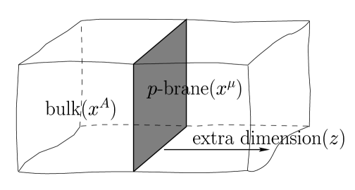
Figure 1: A schematic shape of brane world model: Spatial section of our universe at time $t$ is a brane (shaded region) expressed by coordinates $x^{i}$ and that of higher dimensional bulk embedding our universe (transparent box) is depicted by $x^{A}$. One coordinate $z$ transverse to the brane is extra dimension.

The action of our interest is

$$S=\int d^{D}x\sqrt{g_{D}}\left[-\frac{M^{p}_{*}}{16\pi}(R+2\Lambda)\right]+S_{\rm matter},$$ (2.4)

where $M_{*}$ is the fundamental scale of the theory, $\Lambda$ a cosmological constant, and $S_{{\rm matter}}$ stands for any matter of our interest. We read Einstein equations in the ($p$+2)-dimensional bulk from the action (2.4)

$$G_{AB}\equiv R_{AB}-\frac{1}{2}g_{AB}R=-\frac{8\pi}{M^{p}_{*}}T_{AB}+g_{AB}\Lambda,$$ (2.5)

where energy-momentum tensor $T_{AB}$ in Eq. (2.5) is defined by

$$T_{AB}\equiv\frac{2}{\sqrt{g_{D}}}\,\,\frac{\delta S_{\rm matter}}{\delta g^{AB}}.$$ (2.6)

In this pedagogical review, we take into account the matters restricted to the brane, which coincide with those of original idea [2, 3]. When the matters are confined on a specific $p$-brane, then the metric fluctuation to the $z$-direction so-called radion direction vanishes, i.e., $\delta g^{zz}=0$, and thereby the energy-momentum tensor from the sources confined on the brane becomes

$$T_{AB}^{\rm brane}\equiv\left.\frac{2}{\sqrt{g_{D}}}\,\,\frac{\delta S_{\rm matter}^{\rm brane}}{\delta g^{AB}}\right|_{\delta g^{zz}=0}.$$ (2.7)

When we particularly consider the metric ansatz without the cross terms among time variable $t$, spatial coordinates of the brane $x^{i}$, $(i=1,2,3)$, and coordinate of the extra-dimension $z$, a 5-dimensional metric is expressed as follows, which includes a flat $p=3$ brane and is convenient for the description of the brane world

$$ds^{2}=e^{2A(t,z)}[dt^{2}-D^{2}(t,z)dx^{i2}]-C^{2}(t,z)dz^{2},$$ (2.8)

where $A(t,z)$, $D(t,z)$, and $C(t,z)$ are three real metric functions of $t$ and $z$ [5]. Actually, vanishing off-diagonal metric components in front of $dx^{\mu}dz$ is consistent with the reflection symmetry of the $z$-coordinate for orbifold compactification, i.e., $z\rightarrow-z$. Similar symmetry argument, e.g., time-reversal ($t\rightarrow-t$) or parity ($x^{i}\rightarrow-x^{i}$ for $p$ = 3), is also applied to the $p$-brane, which results in vanishing $dtdx^{i}$ component. If the geometry of our interest is static, Eq. (2.8) becomes

$$ds^{2}=e^{2A(z)}[dt^{2}-D^{2}(z)dx^{i2}]-C^{2}(z)dz^{2}.$$ (2.9)

Introducing a new coordinate $Z$ such as $dZ=C(z)dz$, we rewrite the metric (2.9) as

$$ds^{2}=e^{2A(z(Z))}[dt^{2}-D^{2}(z(Z))dx^{i2}]-dZ^{2}.$$ (2.10)

Eq. (2.10) has two independent metric functions. If we force Poincaré symmetry with the unit light speed for the spacetime of the $p$-brane, then the boost symmetry asks $D^{2}(Z(z))=1$ so that we finally arrive at

$$ds^{2}=e^{2A(Z)}(dt^{2}-dx^{i2})-dZ^{2}=e^{2A(Z)}\eta_{\mu\nu}dx^{\mu}dx^{\nu}-dZ^{2}.$$ (2.11)

On the other hand, when the cosmology is our interest, we have to consider the homogeneous and isotropic $p$-brane. The simplest model is depicted by the metric which involves time-dependence only in front of the 3-brane coordinates, i.e., $D(t,Z)=e^{b(t)}$ :

$$ds^{2}=e^{2A(Z)}[dt^{2}-e^{2b(t)}dx^{i\,2}]-dZ^{2},$$ (2.12)

which leads to Eq. (2.11) in static limit. If a constant curvature consistent with the homogeneity and isotropy is included, we have

$$ds^{2}=e^{2A(Z)}\left[dt^{2}-e^{2b(t)}\left(\frac{dr^{2}}{1-Kr^{2}}+r^{2}d\theta^{2}+r^{2}\sin^{2}\theta d\phi^{2}\right)\right]-dZ^{2},$$ (2.13)

where $K=1$ corresponds to three sphere of unit radius, $K=0$ 3-dimensional flat space, and $K=-1$ three hyperbolic space.

For this metric (2.11), the Einstein equations (2.5) are given by the following simple equations

$$A^{{}^{\prime}2} = \frac{2}{p(p+1)}\left(\frac{8\pi}{M^{p}_{\ast}}T^{Z}_{\;Z}-\Lambda\right),$$ (2.14)

$$A^{\prime\prime} = -\frac{1}{p}\frac{8\pi}{M_{*}^{p}}\left(T_{\;Z}^{Z}-T_{\;t}^{t}\right),\qquad\left(T^{t}_{\;t}=T^{i}_{\;i}\right),$$ (2.15)

where the prime in ${A}^{{}^{\prime}}$ denotes the differentiation by $Z$-coordinate. In order to identify the physical singularity, we look into sum of square of all components of the Riemann curvature tensor so-called the Kretschmann scalar invariant from the metric (2.12)

$$R^{ABCD}R_{ABCD}=2(p+1)\left[pA^{{}^{\prime}4}+2\left(A^{\prime\prime}+A^{\prime 2}\right)^{2}\right].$$ (2.16)

Derivation of the above equations and quantities are given in Appendix B.

A warp coordinate system (2.12) is unusual for the description of anti-de Sitter spacetime so that we introduce familiar logarithmic coordinate such as $dZ\sim\pm dy/\sqrt{B(y)}$ with $B(y)\sim e^{2A(Z)}$. Then the metric (2.12) is rewritten in other coordinates

$$ds^{2}=B(y)(dt^{2}-dx^{i2})-\frac{dy^{2}}{B(y)},$$ (2.17)

and corresponding Einstein equations are

$$B^{{}^{\prime 2}} = \frac{8B}{p(p+1)}\left(\frac{8\pi}{M_{*}^{p}}T^{y}_{y}-\Lambda\right),$$ (2.18)

$$B^{{}^{\prime\prime}} = -\frac{p+2}{p(p+1)}\frac{32\pi}{pM_{*}^{p}}\left(T^{y}_{y}-T^{t}_{t}\right)+\frac{4\Lambda}{p(p+1)},\qquad\left(T^{t}_{t}=T^{i}_{i}\right),$$ (2.19)

where the prime ${}^{{}^{\prime}}$ in this paragraph denotes differentiation by new variable $y$ of extra dimension. Similarly, we read the Kretschmann invariant from the metric (2.17)

$$R^{ABCD}R_{ABCD}=\frac{p+1}{8B^{2}}\left(pB^{{}^{\prime}4}+8B^{{}^{\prime\prime}2}\right).$$ (2.20)

In subsequent sections, we shall discuss Randall-Sundrum type brane world by use of the prepared building blocks.

3 Geometry of Randall-Sundrum Brane World

3.1 Pure anti-de Sitter spacetime

When the bulk is filled only with negative vacuum energy $\Lambda<0$ without other matters $S_{\rm matter}=0$ so that $T_{AB}=0$, then the Einstein equations (2.14)$\sim$(2.15) are

$$A^{{}^{\prime\prime}}=0~{}{\rm{and}}~{}A^{{}^{\prime}2}=-\frac{2\Lambda}{p(p+1)}.$$ (3.1)

Notice that $A(Z)$ can have a real solution only when $\Lambda$ is nonpositive. General solution of Eq.$~{}(\ref{u5s})$ is given by

$$A_{\pm}(Z)=\pm\sqrt{\frac{2|\Lambda|}{p(p+1)}}Z+A_{0},$$ (3.2)

where the integration constant $A_{0}$ can be removed by rescaling of the spacetime variables of $p$-brane, i.e., $dx^{\mu}\rightarrow d\bar{x}^{\mu}=e^{A_{0}}dx^{\mu}$. The resultant metric is

$$ds^{2}=e^{\pm 2kZ}\eta_{\mu\nu}d\bar{x}^{\mu}d\bar{x}^{\nu}-dZ^{2},$$ (3.3)

where $k=\sqrt{2|\Lambda|/p(p+1)}$ and a schematic shape of the metric $e^{2A(Z)}$ is shown in Fig. 2.

Figure 2: The metric function of anti-de Sitter spacetime $e^{2A_{\pm}(Z)}=e^{\pm 2kZ}$.

Since the metric function $e^{2A_{\pm}}$ vanishes or is divergent at spatial infinity $Z=\mp\infty$ respectively, there exists coordinate singularity at those points. Despite of the coordinate singularity, the spacetime is physical-singularity-free everywhere as expected

$$R^{ABCD}R_{ABCD}=\frac{8(p+2)}{p^{2}(p+1)}|\Lambda|^{2}.$$ (3.4)

As mentioned in the previous section, the warp coordinate system (3.3) is unusual to depict geometry of the anti-de Sitter spacetime. A coordinate transformation to the metric (2.17) via $dZ=\alpha dy/y$ leads to

$$ds^{2} = e^{\pm\sqrt{\frac{8|\Lambda|}{p(p+1)}}\ln{\left(\frac{y}{y_{0}}\right)^{\alpha}}}\eta_{\mu\nu}d\bar{x}^{\mu}d\bar{x}^{\nu}-\alpha^{2}\frac{dy^{2}}{y^{2}}$$ (3.5)

$$= y^{\pm\alpha\sqrt{\frac{8|\Lambda|}{p(p+1)}}}\eta_{\mu\nu}d\tilde{x}^{\mu}d\tilde{x}^{\nu}-\alpha^{2}\frac{dy^{2}}{y^{2}}$$ (3.6)

$$= y^{2}\eta_{\mu\nu}d\tilde{x}^{\mu}d\tilde{x}^{\nu}-\alpha^{2}\frac{dy^{2}}{y^{2}}$$ (3.7)

$$= \frac{p(p+1)}{2|\Lambda|}\left(y^{2}\eta_{\mu\nu}dx^{\mu}dx^{\nu}-\frac{dy^{2}}{y^{2}}\right).$$ (3.8)

The integration constant $\ln y_{0}$ in the first line (3.5) was eliminated by rescaling of the spacetime variables of $p$-brane, i.e., $d\tilde{x}^{\mu}=e^{\mp\alpha\sqrt{8|\Lambda|/p(p+1)}\ln y_{0}}d\bar{x}^{\mu}$. The third line (3.7) was obtained by a choice of $\alpha$ as $\pm 2\sqrt{\frac{p(p+1)}{8|\Lambda|}}$. A rescaling of a coordinate $dx^{\mu}=d\tilde{x}^{\mu}/\alpha$ leads to the line (3.8). Because of the coordinate transformation $Z=\ln{y^{\alpha}}$, $Z=\infty$ corresponds to $y=0$ when $\alpha<0$ (or $y=\infty$ when $\alpha>0$) and $Z=0$ to $y=1$ so that the spacetime described by the coordinate system (2.11) does not represent entire anti-de Sitter spacetime but a patch of it as is obvious from the coordinate transformation, $Z=\ln{y^{\alpha}}$. Now the developed coordinate singularity is found at both $y=0$ and $y=\infty$ in the metric (3.8). Of course, the Kretschmann invariant (2.20) is independent of the choice of specific form of the metric so that it is the same as Eq. (3.4). An intriguing observation is that the coordinate singularity at $y=0$ can also be understood as a horizon with zero radius limit (or equivalently zero mass limit) of black $p$-brane.

3.2 Randall-Sundrum brane world II

When we want to use the obtained solutions  (3.2) for compactification of the extra-dimension $\{Z\}$, the metric function should necessarily be single-valued even at infinity $Z=\pm\infty$. A natural method is to urge a reflection symmetry (${\rm Z}_{2}$-symmetry) to $Z$-coordinate so that we can have two continuous solutions in Fig. 3 by patching two solutions (3.2) at the origin $Z=0$. Since we are not interested in exponentially-blowing up solution in Fig. 3-(b), we consider only the exponentially-decreasing warp factor in Fig. 3-(a) from now on. Though it is continuous, it does not satisfy the Einstein equations (3.1) at the origin $Z=0$ as far as we do not assume a singular matter configuration at that point. The curve of the first derivative of $A(Z)$ is given by the step functions

$$A^{{}^{\prime}}_{\rm II}(Z)=-k\left[\theta(Z)-\theta(-Z)\right],$$ (3.9)

and thereby that of second derivative is nothing but a delta function instead of zero as in Eq. (3.1)

$$A^{{}^{\prime\prime}}_{\rm II}(Z)=-2k\delta(Z).$$ (3.10)

Schematic shapes of first and second derivatives of the warp factor $e^{2A_{\rm II}(Z)}$ are shown in Fig. 4.

Figure 3: Continuous Z₂-symmetric anti-de Sitter space : (a) $e^{2A_{\rm II}(Z)}=e^{-2k|Z|}$(solid line), (b) $e^{2A(Z)}=e^{2k|Z|}$ (dashed line).

Figure 4: (a) First derivative of $e^{2A_{\rm II}(Z)}$, (b) second derivative of $e^{2A_{\rm II}(Z)}.$

An appropriate interpretation of the delta function in Eq. (3.10) is to regard it as a matter source confined on the $p$-brane at $Z=0$. Eq. (B.8) tells us that $T^{t}_{\;t}=T^{i}_{\;i}$ for any static metric. Substituting Eq. (3.10) into one of the Einstein equations (2.15), we obtain

$$T^{t}_{{\rm II}\,t}-T^{Z}_{{\rm II}\,Z}=\frac{pkM^{p}_{\ast}}{4\pi}\delta(Z).$$ (3.11)

Insertion of Eq. (3.9) into the $ZZ$-component of the Einstein equation (2.14) provides vanishing $ZZ$-component of the energy-momentum tensor

$$T^{Z}_{{\rm II}\,Z}=\frac{M^{p}_{\ast}|\Lambda|}{8\pi}\left\{[\theta(Z)-\theta(-Z)]^{2}-1\right\}=0.$$ (3.12)

Therefore, we have

$$T^{t}_{{\rm II}\,t}=T^{i}_{{\rm II}\,i}=\frac{M^{p}_{\ast}}{8\pi}2pk\delta(Z),~{}~{}~{}T^{Z}_{{\rm II}\,Z}=0,$$ (3.13)

and corresponding covariant form of it is

$$T^{\;A}_{{\rm II}\,B}=\frac{M^{p}_{\ast}}{8\pi}2pk\delta(Z)\delta^{\mu}_{\;\nu}\delta^{A}_{\;\mu}\delta_{\;B}^{\nu}.$$ (3.14)

This is the result we expected, that is, the delta function source in Eq. (3.10) is indeed a constant matter density on the $p$-brane at the origin. Signature of the energy-momentum tensor (3.14) implies the positiveness of the $p$-brane tension. When the matter is confined on a specific $p$-brane, the metric fluctuation to the radial direction vanishes, i.e. $\delta g^{ZZ}=0$. Therefore the energy-momentum tensor from the sources confined on the $p$-brane becomes

$$T^{\rm brane}_{AB}\equiv\left.\frac{2}{\sqrt{g_{D}}}\frac{\delta S^{\rm brane}_{\rm matter}}{\delta g^{AB}}\right|_{\delta g^{ZZ}=0}.$$ (3.15)

An appropriate form of matter action is written by use of Eq. (2.7) such as

$$S_{\rm II}=\frac{M^{p}_{\ast}}{8\pi}\int d^{p+1}x\int^{\infty}_{-\infty}dZ\sqrt{g_{D}}\,2pk\delta(Z).$$ (3.16)

Note that the above junction condition at the $p$-brane is nothing but a fine-tuning condition since all the contents of the matter action (3.16) should be determined by the quantities of the bulk, specifically by the fundamental scale of the bulk theory $M_{\ast}$ and the bulk cosmological constant $\Lambda$. Since there is no constant density term in the $p$-brane action, the effective cosmological constant on the $p$-brane (or our universe) vanishes.

The resultant metric of Randall-Sundrum brane world model II [3] is

$$ds^{2}=e^{-2k|Z|}\eta_{\mu\nu}d\bar{x}^{\mu}d\bar{x}^{\nu}-dZ^{2}.$$ (3.17)

Once we transform it to the Schwarzschild-type coordinates (2.17) , we can easily find coordinate singularities at both infinity, $Z=\pm\infty$. Since we added the matter on the $p$-brane as a delta function source, the Kretschmann invariant contains a delta function like physical singularity at $Z=0$

$$R^{ABCD}R_{ABCD}=\frac{8}{p}|\Lambda|\left[\frac{|\Lambda|}{p+1}+\left(\sqrt{\frac{2|\Lambda|}{p(p+1)}}-2\delta(Z)\right)^{2}\right].$$ (3.18)

3.3 Randall-Sundrum brane world I

Suppose that the coordinate of the extra-dimension $Z$ is really compact in Randall-Sundrum brane world model I, different from the previous Randall-Sundrum brane world II with $-\infty\leq Z\leq\infty$. An appropriate method from the brane world II to I is attained by forcing periodicity to the coordinate of the extra-dimension $Z$ in addition to the Z₂-symmetry as shown in Fig. 5. It is exactly an orbifold compactification by ${\bf S}^{1}/Z_{2}$ and thereby physics of our interest lives in a compact region $\{Z|[0,r_{\rm c}\pi]\}$. To achieve this geometry by adding matters on the branes at both $Z=0$ and $Z=r_{\rm c}\pi$, we already learned that two delta function sources should be taken into account at both $Z=0$ and $Z=r_{\rm c}\pi$, similar to the action (3.16) :

Figure 5: Metric function $e^{-2A_{\rm I}(Z)}$ for Randall-Sundrum compactification I. There is a hidden brane matter at $Z=0$, and our world in electroweak scale is located at $Z=r_{\rm c}\pi$.

$$S_{\rm I} \equiv S_{\rm I}|_{Z=0}+S_{\rm I}|_{Z=r_{\rm c}\pi}$$ (3.19)

$$= \frac{M^{p}_{\ast}}{8\pi}\int d^{p+1}x\int^{r_{\rm c}\pi}_{-r_{\rm c}\pi}dZ\sqrt{g_{D}}\,2pk[\delta(Z)-\delta(Z-r_{\rm c}\pi)].$$

Then the corresponding energy-momentum tensor restricted on both $p$-branes is computed by the formula (2.7)

$$T^{A}_{{\rm I}\;B}=\frac{M^{p}_{\ast}}{8\pi}2pk[\delta(Z)-\delta(Z-r_{\rm c}\pi)]\delta^{\mu}_{\;\nu}\delta^{A}_{\;\mu}\delta_{\;B}^{\nu},$$ (3.20)

and the Einstein equations (2.14)$\sim$(2.15) become

$$A^{{}^{\prime}}_{\rm I}(Z) = -2k\left[\theta(Z)-\theta(-Z)\right]-2k\left[\theta(Z-r_{\rm c}\pi)-\theta(-Z+r_{\rm c}\pi)\right],$$ (3.21)

$$A^{{}^{\prime\prime}}_{\rm I}(Z) = -2k[\delta(Z)-\delta(Z-r_{\rm c}\pi)].$$ (3.22)

Note that the brane at $Z=0$ has positive tension but the other brane at $Z=r_{\rm c}\pi$ has negative tension. The metric of the Randall-Sundrum brane world I [2] is expressed by

$$ds^{2}=e^{-2kr_{\rm c}\varphi}\eta_{\mu\nu}dx^{\mu}dx^{\nu}-r_{\rm c}^{2}d\varphi^{2},~{}~{}~{}(0\leq\varphi\leq\pi).$$ (3.23)

It is free from coordinate singularity but involves physical singularity at both patched boundaries ($Z=0$ and $Z=r_{\rm c}\pi$):

$$R_{ABCD}R^{ABCD}=\frac{8}{p}|\Lambda|\left\{\frac{|\Lambda|}{p+1}+\left[\sqrt{\frac{2|\Lambda|}{p(p+1)}}-2\left(\delta(Z)-\delta(Z-r_{\rm c}\pi)\right)\right]^{2}\right\}.$$ (3.24)

Again, we encounter the fine-tuning conditions: One is the fine-tuning that the brane matter action is completely determined by the bulk negative cosmological constant $\Lambda$ and the fundamental scale of the bulk theory $M_{\ast}$, and the other is the fine-tuning that the magnitudes of both brane matter actions, $S_{\rm I}|_{Z=0}$ and $S_{\rm I}|_{Z=r_{\rm c}\pi}$, are exactly the same each other but have the opposite sign:

$$\frac{S_{\rm I}|_{Z=0}}{V_{p+1}}=-\frac{S_{\rm I}|_{Z=r_{\rm c}\pi}}{V_{p+1}}=\frac{M^{p}_{\ast}}{8\pi},$$ (3.25)

where the spacetime volume of each $p$-brane is denoted by $V_{p+1}=\int d^{p+1}x$. Therefore, the $p$-brane at the origin has the positive tension but the other brane at $Z=r_{\rm c}\pi$ the negative tension. Note that the effective cosmological constant vanishes on the $p$-branes at both boundaries, $Z=0$ and $Z=r_{\rm c}\pi$.

4 Physical Implication of Randall-Sundrum Brane World

In this section we discuss two main features of Randall-Sundrum brane world models. In the model II with single brane, gravitational fluctuations on the brane reproduce the Newtonian gravity from normalizable zero mode. In the model I with two branes, the gauge hierarchy problem can be treated in a much milder form without assuming supersymmetry.

4.1 Newtonian gravity from model II

In the subsection 3.2, we discussed the Randall-Sundrum brane world model II which can be defined whthin $-\infty\leq Z\leq\infty$. The summary for this RS II model is described by the metric in Eq. (3.17). The aim of this subsection is to determine whether the spectrum of general linerized tensor fluctuations $H_{\mu\nu}$ is consistent with 4-dimensional experimental gravity. To do so, let us consider the small gravitational fluctuations $\delta g_{AB}$ on the given background metric $g_{AB}$.

$$ds^{2}=(g_{AB}+\delta g_{AB})dx^{A}dx^{B}.$$ (4.1)

In present RS model II, we restrict the small fluctuations $\delta g_{AB}$ to the metric $h_{\mu\nu}(x,Z)$ of 4-dimensional world on the 3-brane. The metric in Eq. (4.1) becomes

$$ds^{2}=[e^{-2k|Z|}\eta_{\mu\nu}+h_{\mu\nu}(x,Z)]dx^{\mu}dx^{\nu}-dZ^{2}\equiv H_{\mu\nu}dx^{\mu}dx^{\nu}-dZ^{2},$$ (4.2)

where $H_{\mu\nu}$ stands for the linearized tensor fluctuations. Substituting the metric (4.2) into the Einstein tensor $G_{AB}$ with the help of transverse-traceless gauge where

$$\partial^{\mu}h_{\mu\nu}=0,\qquad h^{\mu}_{\;\mu}=0,$$ (4.3)

we can easily see that the small fluctuations in the Einstein tensor $G_{AB}$ have the nonvanishing components only on the 3-brane as

$$\delta\left(G_{\mu\nu}=-\frac{8\pi}{M^{p}_{\ast}}T_{\mu\nu}+\Lambda g_{\mu\nu}\right)$$

$$\Longrightarrow\hskip 14.22636pt\left[\frac{1}{2}\left(U^{-1}\eta^{\rho\sigma}\partial_{\rho}\partial_{\sigma}-\partial_{Z}^{2}\right)+V(Z)\right]h_{\mu\nu}=0,$$ (4.4)

where

$$V(Z) = 2\left(\frac{U^{\prime\prime}}{U}\right)+6k\delta(Z)-6k^{2},$$ (4.5)

$$U(Z) = e^{-2k|Z|}.$$ (4.6)

See Appendix C for detailed derivation of Eq. (4.4).

To understand all modes that appear in 4-dimensional effective theory, we perform a KK reduction down to four dimensions. To do so, let us summarize the obtained linearized equations for the small fluctuations

$$\left[\frac{1}{2}\left(e^{2k|Z|}\eta^{\rho\sigma}\partial_{\rho}\partial_{\sigma}-\partial_{Z}^{2}\right)-2k\delta(Z)+2k^{2}\right]h_{\mu\nu}(x^{\alpha},Z)=0.$$ (4.7)

Since nontrivial potential part depends only on the 5th-coordinate $Z$, we can easily apply the separation of variables to this linear equation. To be specific, inserting

$$h_{\mu\nu}(x^{\rho},Z)=\psi(Z)\Phi(x^{\rho})$$ (4.8)

into Eq. (4.7), we have

$$\eta^{\mu\nu}\partial_{\mu}\partial_{\nu}\Phi(x^{\rho})=-m^{2}\Phi(x^{\rho}),\qquad(m^{2}\geq 0),$$ (4.9)

$$\left[-\frac{m^{2}}{2}e^{2k|Z|}-\frac{1}{2}\partial_{Z}^{2}-2k\delta(Z)+2k^{2}\right]\psi(Z)=0,$$ (4.10)

where $m$ is the 4-dimensional mass of the KK excitation.

By making a change of variable as follows

$$w = \frac{{\rm sgn}(Z)}{k}(e^{k|Z|}-1),\qquad({\rm sgn}(Z)\equiv Z/|Z|=\theta(Z)-\theta(-Z)),$$ (4.11)

$$\hat{\psi}(w) = e^{k|Z|/2}\psi(Z),$$ (4.12)

we rewrite Eq. (4.10) in a simpler form

$$-\frac{1}{2}\frac{d^{2}\hat{\psi}}{dw^{2}}+\hat{V}(w)\hat{\psi}=\frac{m^{2}}{2}\hat{\psi},$$ (4.13)

where

$$\hat{V}(w)=\frac{15k^{2}}{8(k|w|+1)^{2}}-\frac{3}{2}k\delta(w).$$ (4.14)

Here we used $\delta(w)=\delta(Z)=\frac{1}{2}\frac{d}{dZ}{\rm sgn}(Z)$ and see Fig. 4-(b) for the volcano-type potential $\hat{V}$. Since we have an explicit form of the KK potential  (4.14), we will discuss the properties of continuum modes $m$ in the end of this subsection. Before doing so, however, we would like to give the discussions on the case of zero mode, $m^{2}=0$, in Eq. (4.9).

In the static frame with the rotational symmetry on the 3-brane (or our universe), Eq. (4.9) with $m^{2}=0$ is reduced to the well-known Laplace equation

$$\frac{1}{r^{2}}\frac{d}{dr}\left[r^{2}\frac{d\Phi(r)}{dr}\right]=0.$$ (4.15)

Except for the source point at the origin $r=0$, the Newtonian potential

$$\Phi(r)=-\frac{A}{r}$$ (4.16)

satisfies Eq. (4.15). Here we set $\Phi(\infty)=0$ and $A=G_{{\rm N}}m_{1}m_{2}$ in order to match Newtonian gravity between two particles of mass $m_{1}$ and $m_{2}$ on our brane at $Z=0$. Now that we have Newtonian gravitational potential on the 3-brane, we solve $\psi(Z)$ in the extra dimension. When $m^{2}=0$, we directly deal with Eq. (4.10) given by

$$\frac{d^{2}\psi}{dZ^{2}}=\left[4k^{2}-4k\delta(Z)\right]\psi(Z).$$ (4.17)

For $Z\neq 0$, we have

$$\psi(Z)=\psi_{0}e^{-2k|Z|},$$ (4.18)

which satisfies the boundary condition obtained by integration of Eq. (4.17) for $-\varepsilon\leq Z\leq\varepsilon$ for infinitesimal $\varepsilon$

$$4k\psi(0)=\lim_{\varepsilon\rightarrow 0}\left(\left.\frac{d\psi}{dZ}\right|_{\varepsilon}-\left.\frac{d\psi}{dZ}\right|_{-\varepsilon}\right).$$ (4.19)

Normalization condition $\int_{-\infty}^{\infty}dZ|\psi(Z)|^{2}=1$ fixes the overall constant $\psi_{0}$ as

$$\psi(Z)=\sqrt{2k}e^{-2k|Z|}.$$ (4.20)

With the explicit form of the KK potential (4.14), we can understand the properties of KK modes of $m^{2}\not=0$. Since the KK potential falls off to zero as $|Z|\rightarrow\infty$, the continuum KK states with no gap exist for all possible $m^{2}>0$ and then the proper measure is simply $dm$. For the detailed discussion on the proper measure through the Bessel function representation for the solution of Eq. (4.13) refer to Ref. [3].

With the KK spectrum of the effective 4-dimensional theory, let us compute the gravitational potential $\Phi(r)$ between two particles of mass $m_{1}$ and $m_{2}$ on our brane at $|Z|=0$, which is the static potential generated by exchange of the zero-mode and continuum KK modes propargators;

$$\Phi(r)\approx G_{\rm N}\frac{m_{1}m_{2}}{r}+\frac{G_{\rm N}}{k}m_{1}m_{2}\int_{0}^{\infty}dm\frac{m}{k}\frac{e^{-mr}}{r}.$$ (4.21)

There is a Yukawa potential in the correction term, and an extra factor of $m/k$ comes from the continuum wave functions $\psi(Z)$ for $m^{2}\not=0$ at $Z=0$. The coupling $G_{\rm N}/k$ is nothing but the fundamental coupling of gravity, $1/M_{*}^{3}$. By performing the integration over $r$ in Eq. (4.21), we have a next order correction of $O(1/r^{3})$ to the Newtonian potential

$$\Phi(r)\sim G_{\rm N}\frac{m_{1}m_{2}}{r}\left(1+\frac{1}{k^{2}r^{2}}\right).$$ (4.22)

This is the reason why the RS II model produces an effective 4-dimensional theory of gravity: the leading term is given by the usual Newtonian potential and a continuos KK modes generate a correction term. Note that the radion can be an additional source of $O(1/r^{3})$ contribution [6].

4.2 Gauge hierarchy from model I

As we explained briefly in the introduction, the gauge hierarchy problem is a notorious fine tuning problem in particle phenomenology of which the basic language is quantum field theory. So the readers unfamiliar to field theories may skip this subsection.

Let us assume that we live on the $p$-brane at $Z=r_{\rm c}\pi$ and try a dimensional reduction of the Einstein gravity from the $D=p+2$-dimensional gravity to $p+1$-dimensional gravity on the $p$-brane at $Z=r_{\rm c}\pi$. Then we have

$$S_{{\rm EH}\,D} = -\frac{M_{\ast}^{p}}{16\pi}\int d^{D}x\sqrt{|g_{D}|}\,R$$ (4.23)

$$= -\frac{M_{\ast}^{p}}{16\pi}\int d^{p+1}x\sqrt{|\det g_{\mu\nu}|}\int^{r_{\rm c}\pi}_{-r_{\rm c}\pi}dZe^{-(p-1)k|Z|}(R_{p+1}+\cdots)$$ (4.24)

$$= -\frac{M_{\ast}^{p}}{16k\pi}\left[1-e^{-(p-1)kr_{\rm c}\pi}\right]\int d^{p+1}x\sqrt{|\det g_{\mu\nu}|}\,(R_{p+1}+\cdots)$$ (4.25)

$$\equiv -\frac{M_{\rm Planck}^{2}}{16\pi}\int d^{p+1}x\sqrt{|\det g_{\mu\nu}|}\,(R_{p+1}+\cdots)$$ (4.26)

$$= S_{{\rm EH}\,p+1}+\cdots.$$ (4.27)

We used $g_{D}=e^{-2(p+1)k|Z|}\det g_{\mu\nu}$ and $R=e^{2k|Z|}g^{\mu\nu}R_{\mu\nu}+\cdots=e^{2k|Z|}R_{p+1}+\cdots$ when we calculated the second line (4.24) from the first line (4.23). By comparing the third line (4.25) with the fourth line (4.27), we obtain a relation for $3$-brane among three scales $M_{\rm Planck}$, $M_{\ast}$, $|\Lambda|$ $(p=3)$:

$$M_{\rm Planck}^{2}=\sqrt{\frac{p(p+1)}{2|\Lambda|}}\left[1-\exp\left(-\sqrt{\frac{8|\Lambda|}{p(p+1)}}r_{\rm c}\pi\right)\right]M_{\ast}^{p=3}.$$ (4.28)

A natural choice for the bulk theory is to bring up almost the same scales for two bulk mass scales, i.e., $M_{\ast}\approx\sqrt{|\Lambda|}$. Suppose that the exponential factor in the relation (4.28) is negligible to the unity, which means $r_{\rm c}$ is slightly larger than $1/\sqrt{|\Lambda|}$. Then we reach

$$M_{\rm Planck}\approx M_{\ast}\approx\sqrt{|\Lambda|}.$$ (4.29)

A striking character of this Randall-Sundrum compactification I is that it provides an explanation for gauge hierarchy problem that why is so large the mass gap between the Planck scale $M_{\rm Planck}\sim 10^{19}{\rm GeV}\sim 10^{-38}~{}M_{\odot}$ and the electroweak scale $M_{\rm EW}\sim 10^{3}{\rm GeV}\sim 10^{-54}$ $M_{\odot}$ without assuming supersymmetry or others. As a representative example, let us consider a massive neutral scalar field $H$ which lives on our $3$-brane at $Z=r_{\rm c}\pi$ :

$$S_{\rm scalar} = \int^{r_{\rm c}\pi}_{-r_{\rm c}\pi}dZ\delta(Z-r_{\rm c}\pi)\int d^{4}x\sqrt{g_{5}}\Biggl{[}\frac{1}{2}g^{AB}\partial_{A}H\partial_{B}H-\frac{1}{2}M^{2}_{{\rm Planck}}H^{2}\Biggr{]}$$ (4.30)

$$= \int^{r_{\rm c}\pi}_{-r_{\rm c}\pi}dZe^{-4k|Z|}\delta(Z-r_{\rm c}\pi)\int d^{4}x\sqrt{-\hat{g}_{4}}$$

$$\hskip 28.45274pt\times\Biggl{[}\frac{1}{2}e^{2k|Z|}\hat{g}^{\mu\nu}\partial_{\mu}H\partial_{\nu}H-\frac{1}{2}M^{2}_{{\rm Planck}}H^{2}-\frac{1}{2}\hat{g}^{ZZ}\left(\partial_{Z}H\right)^{2}\Biggr{]}$$

$$= e^{-2r_{\rm c}\pi k}\int d^{4}x\sqrt{-\hat{g}_{4}}\Biggl{[}\frac{1}{2}\hat{g}^{\mu\nu}\partial_{\mu}H\partial_{\nu}H-\frac{1}{2}(e^{-r_{\rm c}\pi k}M_{{\rm Planck}})^{2}H^{2}\Biggr{]}$$

$$= e^{-2r_{\rm c}\pi k}\int d^{4}x\sqrt{-\hat{g}_{4}}\Biggl{[}\frac{1}{2}\hat{g}^{\mu\nu}\partial_{\mu}H\partial_{\nu}H-\frac{1}{2}M_{{\rm EW}}^{2}H^{2}\Biggr{]},$$ (4.31)

where $ds^{2}=g_{AB}dx^{A}dx^{B}=e^{-2k|Z|}\hat{g}_{\mu\nu}dx^{\mu}dx^{\nu}-dZ^{2}$. The last two lines give us a relation:

$$\frac{M_{\rm EW}}{M_{\rm Planck}}=\exp\left(-\sqrt{\frac{2|\Lambda|}{p(p+1)}}r_{\rm c}\pi\right)\sim 10^{-16}.$$ (4.32)

Therefore, the radius $r_{\rm c}$ of compactified extra dimension of the Randall-Sundrum brane world model I is determined nearly by the Planck scale :

$$\frac{1}{r_{\rm c}}\sim\frac{\pi}{16\sqrt{6}\ln 10}\sqrt{|\Lambda|}\sim\frac{M_{\rm Planck}}{30}.$$ (4.33)

All the scales such as the fundamental scale of the bulk $M_{\ast}$, the bulk cosmological constant $\sqrt{|\Lambda|}$, the inverse size of the compactification $1/r_{\rm c}$, are almost the Planck scales $M_{\rm Planck}\sim 10^{19}$ GeV together. The masses of matter particles on our visible brane at $Z=r_{\rm c}\pi$ are in electroweak scale $M_{\rm EW}\sim 10^{3}$ GeV, however those on the hidden brane at $Z=0$ in the Planck scale. Though the gauge hierarchy problem seems to be solved, it is actually not because a fine-tuning condition was urged in Eq. (3.25). However, it becomes much milder than that before.

How about a massive gauge field $A_{\mu}$ which lives on our $3$-brane at $Z=r_{\rm c}\pi$? We have

$$S_{\rm gauge} = \int^{r_{\rm c}\pi}_{-r_{\rm c}\pi}dZ\delta(Z-r_{\rm c}\pi)\int d^{4}x\sqrt{g_{5}}\Biggl{[}-\frac{1}{4}g^{AC}g^{BD}F_{AB}F_{CD}+M^{2}_{\rm Planck}g^{AB}A_{A}A_{B}\Biggr{]}$$ (4.34)

$$= \int^{r_{\rm c}\pi}_{-r_{\rm c}\pi}dZe^{-4k|Z|}\delta(Z-r_{\rm c}\pi)\int d^{4}x\sqrt{-\hat{g}_{4}}$$

$$\hskip 5.69054pt\times\Biggl{[}-\frac{1}{4}e^{4k|Z|}\hat{g}_{\mu\rho}\hat{g}_{\nu\lambda}F_{\mu\nu}F_{\rho\lambda}+M^{2}_{\rm Planck}e^{2k|Z|}\hat{g}^{\mu\nu}A_{\mu}A_{\nu}\Biggr{]}$$

$$= \int d^{4}x\sqrt{-\hat{g}_{4}}\Biggl{[}-\frac{1}{4}\hat{g}^{\mu\rho}\hat{g}^{\nu\sigma}F_{\mu\nu}F_{\rho\sigma}+(e^{-r_{\rm c}\pi k}M_{\rm Planck})^{2}\hat{g}^{\mu\nu}A_{\mu}A_{\nu}\Biggr{]}$$

$$= \int d^{4}x\sqrt{-\hat{g}_{4}}\Biggl{[}-\frac{1}{4}\hat{g}^{\mu\rho}\hat{g}^{\nu\sigma}F_{\mu\nu}F_{\rho\sigma}+m^{2}_{\rm gauge}\hat{g}^{\mu\nu}A_{\mu}A_{\nu}\Biggr{]}.$$ (4.35)

From Eq. (4.34) and Eq. (4.35) with Eq. (4.32), we read exactly the same mass hierarchy for the gauge field: $m_{\rm gauge}=e^{-r_{\rm c}\pi k}M_{\rm Planck}=M_{\rm EM}$. Therefore the gauge hierarchy can be interpreted by introducing the massive gauge field similar to the case of the massive neutral scalar field $H$.

Finally let us consider a fermionic field of which mass is provided by spontaneous symmetry breaking and its Lagrangian is

$${\cal L}_{\rm fermion}=\bar{\Psi}\gamma^{A}\nabla_{A}\Psi+g\phi\bar{\Psi}\Psi,$$ (4.36)

where $g$ is the coupling constant of Yukawa interaction. If we neglect the quantum fluctuation $\delta\phi$ of $\phi$, i.e. $\phi\equiv\left<\phi\right>+\delta\phi$, the Lagrangian (4.36) becomes

$${\cal L}_{\rm fermion}=\bar{\Psi}\gamma^{A}\nabla_{A}\Psi+g\left<\phi\right>\bar{\Psi}\Psi+\cdots,$$ (4.37)

where the second term is identified as mass term, and we neglected the vertex term $g\delta\phi\bar{\Psi}\Psi$ because we are not interested in quantum fluctuation. Again the fermion lives on our 3-brane at $Z=r_{\rm c}\pi$, and then the action is

$$S_{\rm fermion}=\int^{r_{\rm c}\pi}_{r_{\rm c}\pi}dZ\delta(Z-r_{\rm c}\pi)\int d^{4}x\sqrt{g_{5}}\left[\bar{\Psi}\gamma^{a}e^{A}_{a}\nabla_{A}\Psi+M_{\rm Planck}\bar{\Psi}\Psi\right],$$ (4.38)

where $e^{A}_{a}$ is vielbein defined by $g_{AB}=\eta_{ab}e^{a}_{A}e^{b}_{B}$ and $M_{\rm Planck}=g\left<\phi\right>$ since the symmetry breaking scale should coincide with the fundamental scale. Subsequently, the action (4.38) becomes

$$S_{\rm fermion} = \int^{r_{\rm c}\pi}_{r_{\rm c}\pi}dZ\delta(Z-r_{\rm c}\pi)\int d^{4}x\sqrt{g_{5}}\Big{[}\bar{\Psi}\gamma^{a}e^{A}_{a}\nabla_{A}\Psi+M_{\rm Planck}\bar{\Psi}\Psi\Bigr{]}$$ (4.39)

$$= \int^{r_{\rm c}\pi}_{-r_{\rm c}\pi}dZe^{-4k|Z|}\delta(Z-r_{\rm c}\pi)\int d^{4}x\sqrt{-\hat{g}_{4}}$$

$$\hskip 19.91692pt\times\Bigl{[}e^{k|Z|}\bar{\Psi}\gamma^{a}\hat{e}^{\mu}_{a}\nabla_{\mu}\Psi-\bar{\Psi}\gamma^{a}\hat{e}^{Z}_{a}\nabla_{Z}\Psi+M_{\rm Planck}\bar{\Psi}\Psi\Bigr{]}$$

$$= e^{-3r_{\rm c}\pi k}\int d^{4}x\sqrt{-\hat{g}_{4}}\,\Bigl{[}\bar{\Psi}\gamma^{a}\hat{e}^{\mu}_{a}\nabla_{\mu}\Psi+(e^{-r_{\rm c}\pi k}M_{\rm Planck})\bar{\Psi}\Psi\Bigr{]}$$

$$= e^{-3r_{\rm c}\pi k}\int d^{4}x\sqrt{-\hat{g}_{4}}\,\Bigl{[}\bar{\Psi}\gamma^{a}\hat{e}^{\mu}_{a}\nabla_{\mu}\Psi+m_{\rm fermion}\bar{\Psi}\Psi\Bigr{]}.$$ (4.40)

Once again we obtain the same mass hierarchy relation $m_{\rm fermion}=e^{-r_{\rm c}\pi k}M_{\rm Planck}=M_{\rm EW}$ for the fermion from Eq. (4.39) and Eq. (4.40) with the help of Eq. (4.32).

In this subsection, we demonstrate how to understand the gauge hierarchy problem in the context of Randall-Sundrum brane world model I.

5 Concluding Remarks

In this review, we explained original idea of Randall-Sundrum brane world models I and II. RS I provided a geometrical resolution based on the warp factor to make the gauge hierarchy problem much milder. Though the bulk of RS II contains negative bulk cosmological constant, its effect is cancelled by adjusting the 3-brane tension and then Newtonian gravity is reproduced in weak gravity limit with subleading KK modes on the 3-brane identified as our universe.

Let us conclude by providing some information on a several research topics in this field. They include the problem finding general form of RS solution [5], the stability of brane world model including radion [6], a variety of brane world models basically similar to RS models [7], cosmological implication of RS model including reproduction of standard cosmology [8], construction of thick brane world particularly in terms of solitonic object [9], finding supersymmetry in brane world [10], RS model in the context of string theory [11], brane world with extra dimensions more than one [12], implication to particle phenomenology [13], classical solutions which self-tune the cosmological constant [14], and CMB anisotropy study in brane world [15].

Appendix A Units and Notations

For convenience, we summarize the unit system and the various quantities in this appendix. Our unit system is based on $\hbar(\equiv h/2\pi)=c=1$. Since the light speed $c$ is set to be one, mass of a particle $M$ and its rest energy $Mc^{2}$ have the same unit. Since $c=3\times 10^{8}$m/sec and 1J=1kg m²/sec² $\sim 10^{19}$eV, we have 1kg$\sim 10^{27}$GeV. Astronomical unit of mass is expressed by solar mass $M_{\odot}\sim 2\times 10^{30}$kg. Mass scales are given in Table 1.

mass	particle	daily	astronomy $\&$
scale	physics	life	astrophysics
Planck	$M_{{\rm Planck}}\sim 10^{19}$GeV	$\sim 10^{-8}$kg	$\sim 10^{-38}M_{\odot}$
Electroweak	$M_{\rm EW}\sim 10^{3}$GeV	$\sim 10^{-24}$kg	$\sim 10^{-54}M_{\odot}$

Our basic conversion relation is

$$\hbar c\approx 2\times 10^{-16}{\rm GeV}\cdot{\rm m}.$$ (A.1)

Therefore, uncertainty principle $\Delta E(c\Delta t)\sim\hbar c$ tells us corresponding length scale of quantum physics for given mass scales as shown in Table 2. Here ‘1 pc’ denotes 1 parsec with 1 pc=$3\times 10^{16}$m.

length	daily	astronomy $\&$
scale	life	astrophysics
$1/M_{{\rm Planck}}$	$10^{-35}$m	$10^{-52}$pc
$1/M_{{\rm EM}}$	$10^{-19}$m	$10^{-36}$pc

Our spacetime signature is $(+,-,-,-,-)$ and definitions of the various quantities we use are displayed in the following Table 3.

quantity	definition
Jacobian factor	$g\equiv\det(g_{\mu\nu})$
connection	$\Gamma^{\mu}_{\nu\rho}\equiv\frac{1}{2}g^{\mu\sigma}(\partial_{\nu}g_{\sigma\rho}+\partial_{\rho}g_{\sigma\nu}-\partial_{\sigma}g_{\nu\rho})$
covariant derivative of a contravariant vector	$\nabla_{\mu}A^{\nu}\equiv\partial_{\mu}A^{\nu}+\Gamma^{\nu}_{\mu\rho}A^{\rho}$
Riemann curvature tensor	$R^{\mu}_{\;\;\nu\rho\sigma}\equiv\partial_{\rho}\Gamma^{\mu}_{\sigma\nu}-\partial_{\sigma}\Gamma^{\mu}_{\rho\nu}+\Gamma^{\mu}_{\rho\tau}\Gamma^{\tau}_{\sigma\nu}-\Gamma^{\mu}_{\sigma\tau}\Gamma^{\tau}_{\rho\nu}$
Ricci tensor	$R_{\mu\nu}\equiv R^{\rho}_{\;\mu\rho\nu}$
curvature scalar	$R\equiv g^{\mu\nu}R_{\mu\nu}$
Einstein tensor	$\displaystyle{G_{\mu\nu}\equiv R_{\mu\nu}-\frac{g_{\mu\nu}}{2}R}$

Appendix B Einstein Equations and Geodesic Equations

In this appendix we present detailed calculation of deriving Einstein equations, geodesic equations, and Kretschmann invariant for the metrics used in the description of Randall-Sundrum brane world scenarios by using the formulas in Appendix A.

For the metric (2.12) of warp coordinates, nonvanishing components of the connection are

$$\Gamma^{t}_{tZ}=\Gamma^{x^{i}}_{x^{i}Z}=A^{{}^{\prime}},~{}~{}\Gamma^{t}_{x^{i}x^{i}}=e^{2b}\,\dot{b},~{}~{}\Gamma^{x^{i}}_{tx^{i}}=\dot{b},~{}~{}\Gamma^{Z}_{tt}=e^{2A}A^{{}^{\prime}},~{}~{}\Gamma^{Z}_{x^{i}x^{i}}=-e^{2A+2b}A^{{}^{\prime}}.$$ (B.1)

Nonvanishing components of the Riemann curvature tensor are

$$R^{t}\,_{x^{i}tx^{i}}=-e^{2b}(e^{2A}A^{{}^{\prime}2}-\dot{b}^{2}-\ddot{b}),~{}~{}R^{t}\,_{ZtZ}=R^{x^{i}}\,_{Zx^{i}Z}=-A^{{}^{\prime}2}-A^{{}^{\prime\prime}},$$

$$R^{x^{i}}\,_{ttx^{i}}=-e^{2A}A^{{}^{\prime}2}+\dot{b}^{2}+\ddot{b},~{}~{}R^{Z}\,_{x^{i}x^{i}Z}=e^{2A+2b}(A^{{}^{\prime}}+A^{{}^{\prime\prime}}),$$

$$R^{x^{i}}\,_{x^{j}x^{i}x^{j}}=-e^{2b}(e^{2A}A^{{}^{\prime}2}-\dot{b}^{2}),~{}~{}R^{x^{i}}\,_{x^{j}x^{j}x^{i}}=e^{2b}(e^{2A}A^{{}^{\prime}2}-\dot{b}^{2}),$$

$$R^{Z}\,_{ttZ}=-e^{2A}(A^{{}^{\prime}2}+A^{{}^{\prime\prime}}),$$ (B.2)

and those of Ricci tensor are

$$R_{tt}=(p+1)e^{2A}A^{{}^{\prime}2}-p\dot{b}^{2}+e^{2A}A^{{}^{\prime\prime}}-p\ddot{b},$$

$$R_{x^{i}x^{i}}=-e^{2b}[(p+1)e^{2A}A^{{}^{\prime}2}-p\dot{b}^{2}+e^{2A}A{{}^{\prime\prime}}-\ddot{b}],~{}~{}R_{ZZ}=-(p+1)(A^{{}^{\prime}2}+A^{{}^{\prime\prime}}).$$ (B.3)

Finally the curvature scalar is

$$R=2e^{-2A}\left[\frac{(p+1)(p+2)}{2}e^{2A}A^{{}^{\prime}2}-\frac{p(p+1)}{2}\dot{b}^{2}+(p+1)e^{2A}A^{{}^{\prime\prime}}-p\ddot{b}\right].$$ (B.4)

From Eqs. (B)–(B.4), nonvanishing components of the Einstein equations (2.5) are in arbitrary $D$-dimensions

$$G^{t}_{t} = \frac{p(p-1)}{2}\dot{b}^{2}e^{-2A}-\frac{p(p+1)}{2}{A^{\prime}}^{2}-p{A^{\prime\prime}}=-\frac{8\pi}{M_{*}^{p}}T^{t}_{\;t}+\Lambda\,,$$ (B.5)

$$G^{i}_{i} = (p-1)\ddot{b}e^{-2A}+\frac{p(p-1)}{2}\dot{b}^{2}e^{-2A}-\frac{p(p+1)}{2}{A^{\prime}}^{2}-p{A^{\prime\prime}}=-\frac{8\pi}{M_{*}^{p}}T^{i}_{\;i}+\Lambda\,,$$ (B.6)

$$G^{Z}_{Z} = p\ddot{b}e^{-2A}+\frac{p(p+1)}{2}\dot{b}^{2}e^{-2A}-\frac{p(p+1)}{2}{A^{\prime}}^{2}=-\frac{8\pi}{M_{*}^{p}}T^{Z}_{\;Z}+\Lambda\,.$$ (B.7)

Simplifying the above equations (B.5)$\sim$(B.7), we have

$${(1-p)\ddot{b}}e^{-2A} = -\frac{8\pi}{M_{*}^{p}}\left(T^{t}_{\;t}-T^{i}_{\;i}\right)\,,$$ (B.8)

$$p(\ddot{b}+\dot{b}^{2})e^{-2A}+pA^{\prime\prime} = -\frac{8\pi}{M_{*}^{p}}\left(T_{\;Z}^{Z}-T_{\;t}^{t}\right)\,,$$ (B.9)

$$-\left(\frac{2}{p+1}\ddot{b}+\dot{b}^{2}\right)e^{-2A}+A^{{}^{\prime}2} = \frac{2}{p(p+1)}\left(\frac{8\pi}{M^{p}_{\ast}}T^{Z}_{\;Z}-\Lambda\right).$$ (B.10)

Once we turn off the time-dependence of the scale factor $b(t)$, Eqs. (B.8)–(B.10) become Eqs. (2.14)–(2.15).

Structure of a fixed curved spacetime is usually probed by classical motions of a test particle. Once we obtain geometry of a brane world, then motions of a classical test particle in the given background gravity $g_{AB}$ of the $D$-dimensional bulk are described by geodesic equations

$$\frac{d^{2}x^{A}}{ds^{2}}+\Gamma^{A}_{BC}\frac{dx^{B}}{ds}\frac{dx^{C}}{ds}=0,$$ (B.11)

where the parameter $s$ is chosen by the proper time itself, a force-free test particle moves on a geodesic. For the metric with warp factor (2.12), nontrivial components of the geodesic equations (B.11) are

$$\frac{d^{2}t}{ds^{2}}+A^{{}^{\prime}}\frac{dt}{ds}\frac{dZ}{ds}+\dot{b}e^{2b}\left(\frac{dx^{i}}{ds}\right)^{2}=0,$$ (B.12)

$$\frac{d^{2}x^{i}}{ds^{2}}+A^{{}^{\prime}}\frac{dx^{i}}{ds}\frac{dZ}{ds}+\dot{b}\frac{dt}{ds}\frac{dx^{i}}{ds}=0,$$ (B.13)

$$\frac{d^{2}Z}{ds^{2}}+e^{2A}A^{{}^{\prime}}\left(\frac{dt}{ds}\right)^{2}-e^{2A+2b}A^{{}^{\prime}}\left(\frac{dx^{i}}{ds}\right)^{2}=0.$$ (B.14)

The Kretschmann invariant is

$$R^{ABCD}R_{ABCD}=4p\!\left[(\ddot{b}+\dot{b}^{2})e^{-2A}\!\!\!-A^{{}^{\prime}2}\right]^{2}\!\!+2p(p-1)\left(\dot{b}^{2}e^{-2A}\!\!\!-A^{{}^{\prime}2}\right)^{2}\!\!+4(p+1)(A^{{}^{\prime\prime}}+A^{{}^{\prime}2})^{2},$$ (B.15)

which reduces to Eq. (2.16) in its static limit.

Let us repeat calculation for the Schwarzschild-type metric

$$ds^{2}=B(y)[dt^{2}-e^{2b(t)}dx^{i2}]-\frac{dy^{2}}{B(y)}.$$ (B.16)

We have nonvanishing components of the connection

$$\Gamma^{t}_{ty}=\Gamma^{x^{i}}_{x^{i}y}=\frac{B^{{}^{\prime}}}{2B},~{}~{}\Gamma^{y}_{yy}=-\frac{B^{{}^{\prime}}}{2B},~{}~{}\Gamma^{t}_{x^{i}x^{i}}=e^{2b}\dot{b},$$

$$\Gamma^{x^{i}}_{tx^{i}}=\dot{b},~{}~{}\Gamma^{y}_{tt}=\frac{1}{2}BB^{{}^{\prime}},~{}~{}\Gamma^{y}_{x^{i}x^{i}}=-\frac{e^{2b}}{2}BB^{{}^{\prime}}.$$ (B.17)

Nonvanishing components of the Riemann curvature tensor are

$$R^{t}_{x^{i}tx^{i}}=\frac{e^{2b}}{4}(4\dot{b}^{2}-B^{{}^{\prime}2}+4\ddot{b}),~{}~{}R^{t}\,_{yty}=R^{x^{i}}\,_{yx^{i}y}=-\frac{B^{{}^{\prime\prime}}}{2B}$$

$$R^{x^{i}}\,_{ttx^{i}}=\frac{1}{4}(4\dot{b}-B^{{}^{\prime}2}+4\ddot{b}),~{}~{}R^{x^{i}}\,_{x^{j}x^{i}x^{j}}=\frac{e^{2b}}{4}(4\dot{b}^{2}-B^{{}^{\prime}2}),$$

$$R^{x^{i}}\,_{x^{j}x^{j}x^{i}}=-\frac{e^{2b}}{4}(4\dot{b}^{2}-B^{{}^{\prime}2}),~{}~{}R^{y}\,_{tty}=-\frac{1}{2}BB^{{}^{\prime\prime}},~{}~{}R^{y}\,_{x^{i}x^{i}y}=\frac{e^{2b}}{2}BB^{{}^{\prime\prime}},$$ (B.18)

and those of the Ricci tensor are

$$R_{tt}=\frac{1}{4}(-4p\dot{b}^{2}+pB^{{}^{\prime}2}-4p\ddot{b}+2BB^{{}^{\prime\prime}}),~{}~{}R_{x^{i}x^{i}}=\frac{e^{2b}}{4}(4p\dot{b}^{2}-pB^{{}^{\prime}2}+4\ddot{b}-2BB^{{}^{\prime\prime}}),$$

$$R_{yy}=-\frac{(p+1)B^{{}^{\prime\prime}}}{2B}.$$ (B.19)

The curvature scalar is

$$R=\frac{-4p(p+1)\dot{b}^{2}+p(p+1)B^{{}^{\prime}2}-8p\ddot{b}+4(p+1)BB^{{}^{\prime\prime}}}{4B}.$$ (B.20)

Again, we read the $D$-dimensional Einstein equations (2.5) under this metric

$$G^{t}_{t} = \frac{p(p-1)}{2B}{\dot{b}}^{2}-\frac{p(p-1)}{8}\frac{B^{\prime 2}}{B}-\frac{p}{2}B^{\prime\prime}=-\frac{8\pi}{M_{*}^{p}}T^{t}_{t}+\Lambda,$$ (B.21)

$$G^{i}_{i} = \frac{p-1}{B}\ddot{b}+\frac{p(p-1)}{2B}\dot{b}^{2}-\frac{p(p-1)}{8}\frac{{B^{\prime}}^{2}}{B}-\frac{p}{2}B^{\prime\prime}=-\frac{8\pi}{M_{*}^{p}}T^{i}_{i}+\Lambda,$$ (B.22)

$$G^{y}_{y} = \frac{p}{B}\ddot{b}+\frac{p(p+1)}{2B}\dot{b}^{2}-\frac{p(p+1)}{8}\frac{B^{\prime 2}}{B}=-\frac{8\pi}{M_{*}^{p}}T^{y}_{y}+\Lambda.$$ (B.23)

Then the simplified Einstein equations are

$$\frac{(1-p)\ddot{b}}{B} = -\frac{8\pi}{M_{*}^{p}}\left(T^{t}_{t}-T^{i}_{i}\right),$$ (B.24)

$$\frac{4}{p}\left(\ddot{b}+\dot{b}^{2}\right)+B^{{}^{\prime}2}+2B^{{}^{\prime\prime}}B = -\frac{32\pi}{pM_{*}^{p}}B\left(T^{y}_{y}-T^{i}_{i}\right),$$ (B.25)

$$-4\left(\frac{2\ddot{b}}{p+1}+\dot{b}^{2}\right)+B^{{}^{\prime 2}} = \frac{8B}{p(p+1)}\left(\frac{8\pi}{M_{*}^{p}}T^{y}_{y}-\Lambda\right).$$ (B.26)

Their static limit coincides with Eqs. (2.18)–(2.19).

Nontrivial components of the geodesic equations (B.11) are given by

$$\frac{d^{2}t}{ds^{2}}+\frac{B^{{}^{\prime}}}{2B}\frac{dt}{ds}\frac{dy}{ds}+e^{2b}\dot{b}\left(\frac{dx^{i}}{ds}\right)^{2}=0,$$ (B.27)

$$\frac{d^{2}x^{i}}{ds}+\frac{B^{{}^{\prime}}}{2B}\frac{dx^{i}}{ds}\frac{dy}{ds}+\dot{b}\frac{dt}{ds}\frac{dx^{i}}{ds}=0,$$ (B.28)

$$\frac{d^{2}y}{ds^{2}}+\frac{BB^{{}^{\prime}}}{2}\left(\frac{dt}{ds}\right)^{2}-e^{2b}BB^{{}^{\prime}}\left(\frac{dx^{i}}{ds}\right)^{2}-\frac{B^{{}^{\prime}}}{2B}\left(\frac{dy}{ds}\right)^{2}=0.$$ (B.29)

Similarly, we read the Kretschmann invariant under the metric (B.16)

$$R^{ABCD}R_{ABCD}=\frac{1}{B^{2}}\left[4p\left(\ddot{b}+\dot{b}^{2}-\frac{B^{{}^{\prime}2}}{4}\right)^{2}+2p(p-1)\left(\dot{b}^{2}-\frac{B^{{}^{\prime}2}}{4}\right)^{2}+(p+1)B^{{}^{\prime\prime}2}\right].$$ (B.30)

Its static limit reproduces Eq. (2.20).

Appendix C Small Gravitational Fluctuations

In this appendix, we will give the detailed derivation for Eq. (4.7). Let us consider the variation of the Einstein equations (2.5)

$$\delta\left(G_{AB}=-\frac{8\pi}{M^{p}_{\ast}}T_{AB}+\Lambda g_{AB}\right),$$ (C.1)

where

$$\delta G_{AB}\equiv\delta(R_{AB}-\frac{1}{2}g_{AB}R)=\delta R_{AB}-\frac{1}{2}\delta g_{AB}R.$$ (C.2)

The variation of Ricci tensor in Eq. (C.2) is given by

$$\delta R_{AB}=\nabla_{B}\delta C^{C}_{CA}-\nabla_{C}\delta C^{C}_{AB}\,,$$ (C.3)

where, for small fluctuations, $C^{A}_{BC}$ is

$$\delta C^{D}_{AB}\equiv\frac{1}{2}g^{AD}(\nabla_{B}\delta g_{CD}+\nabla_{C}\delta g_{BD}-\nabla_{D}\delta g_{BC}).$$ (C.4)

From here on we derive Eqs. (C.3)–(C.4). If we consider variation of the covariant derivative for a vector as

$$(\delta\nabla_{A})V_{B}=\tilde{\nabla}_{A}V_{B}-\nabla_{A}V_{B}\equiv-C^{C}_{AB}V_{C}\,,$$ (C.5)

where the tilde over the covariant derivative denotes the quantity calculated on the basis of the perturbed metric $\tilde{g}_{AB}=g_{AB}+\delta g_{AB}$. After some straightforward calculations of $C^{A}_{BC}$ from its definition, we have

$$-C^{C}_{AB}V_{C}=(-\tilde{\Gamma}^{C}_{AB}+\Gamma^{C}_{AB})V_{C},$$ (C.6)

so that

$$C^{C}_{AB}=\frac{1}{2}\tilde{g}^{CD}(\nabla_{A}\tilde{g}_{BD}+\nabla_{B}\tilde{g}_{AD}-\nabla_{D}\tilde{g}_{AB}).$$ (C.7)

For small gravitational fluctuations, Eq. (C.7) coincides with Eq. (C.4).

From the definition of Riemann tensor $[\nabla_{A},\nabla_{B}]V_{C}\equiv V_{D}R^{D}_{CBA}$, we obtain an expression of small variation of the Riemann curvature tensor

$$V_{D}\delta R^{D}_{CBA}=\delta([\nabla_{A},\nabla_{B}])V_{C}\\ =(\nabla_{B}\delta C^{D}_{AC}-\nabla_{A}\delta C^{D}_{BC})V_{D}\,,$$ (C.8)

which leads to

$$\delta R^{D}_{CBA}=\nabla_{B}\delta C^{D}_{AC}-\nabla_{A}\delta C^{D}_{BC}\,.$$ (C.9)

Contraction of two indices provides that of the Ricci tensor in Eq. (C.3).

Now specific computation of fluctuation equations for Eqs. (4.2)–(4.3) is in order. Variation of the Ricci tensor (C.3) is calculated by using the expression of $C^{P}_{MN}$ (C.4)

$$\delta R_{AB} = \frac{1}{2}\nabla_{B}\nabla_{A}\delta g^{C}_{C}-\frac{1}{2}\nabla^{C}(\nabla_{B}\delta g_{AC}+\nabla_{A}\delta g_{BC}-\nabla_{C}\delta g_{AB})\,,$$ (C.10)

$$\delta R_{\mu\nu} = \frac{1}{2}\nabla^{2}h_{\mu\nu}+\frac{1}{2}\nabla_{\mu}\nabla_{\nu}h-\frac{1}{2}\nabla^{A}(\nabla_{\mu}h_{\nu A}+\nabla_{\nu}h_{\mu A})\,,$$ (C.11)

where $h_{\mu\nu}=\delta g_{\mu\nu}$ and $h=h^{\mu}_{\mu}=\delta g^{\mu}_{\mu}$. Note that

$$U^{\prime}=\frac{dU}{dZ},\qquad U^{\prime\prime}=\frac{d^{2}U}{dZ^{2}}.$$ (C.12)

Under the transverse-traceless gauge (4.3), we obtain an expression for variation of the Ricci tensor

$$\delta R_{\mu\nu}=\frac{1}{2}\left(g^{\rho\sigma}\partial_{\rho}\partial_{\sigma}-\partial^{2}_{Z}\right)h_{\mu\nu}-\frac{1}{2}\left(\frac{U^{\prime}}{U}\right)^{2}h_{\mu\nu}.$$ (C.13)

Here we used nonvanishing components of the connection before turning on the fluctuations, which should have only one $Z$ index

$$\Gamma^{Z}_{\mu\nu}=\frac{1}{2}U^{\prime}\eta_{\mu\nu},\qquad\Gamma^{\mu}_{Z\nu}=\frac{1}{2}\left(\frac{U^{\prime}}{U}\right)\delta^{\mu}_{\;\nu}.$$ (C.14)

Substituting the scalar curvature

$$R=-4\left(\frac{U^{\prime\prime}}{U}\right)-\left(\frac{U^{\prime}}{U}\right)^{2},$$ (C.15)

we obtain the variation of gravity part, the left-hand side of the Einstein equations (C.2)

$$\delta(R_{\mu\nu}-\frac{1}{2}g_{\mu\nu}R) = \delta R_{\mu\nu}-\frac{1}{2}h_{\mu\nu}R$$ (C.16)

$$= \frac{1}{2}\left(g^{\rho\sigma}\partial_{\rho}\partial_{\sigma}-\partial^{2}_{Z}\right)h_{\mu\nu}+2\left(\frac{U^{\prime\prime}}{U}\right)^{2}h_{\mu\nu}.$$ (C.17)

Variation of the matter part, the right-hand side of the Einstein equations, is

$$\delta\left(-\frac{8\pi}{M^{p}_{\ast}}T_{AB}+\Lambda g_{AB}\right)=-\frac{8\pi}{M^{p}_{\ast}}\delta T_{AB}+\Lambda\delta g_{AB}.$$ (C.18)

From form of the matter source (3.14), we read

$$\delta T_{ZZ}=0,\qquad\delta T_{\mu\nu}=\frac{M^{p}_{\ast}}{8\pi}2pk\delta(Z)h_{\mu\nu},$$ (C.19)

where we used the relation $T_{AB}=g_{AC}T^{C}_{B}$. By comparing Eq. (C.17) and Eq. (C.18), we finally arrive at the Einstein equations for the small gravitational fluctuations (4.7).

References

- [1] N. Arkani-Hamed, S. Dimopoulos and G. Dvali, Phys. Lett. B 429, 263 (1998) [hep-ph/9803315]; Phys. Rev. D 59, 086004 (1999), [hep-ph/9807344]; I. Antoniadis, N. Arkani-Hamed, S. Dimopoulos and G. Dvali, Phys. Lett. B 436, 257 (1998), [hep-ph/9804398].
- [2] L. Randall and R. Sundrum, Phys. Rev. Lett. 83, 3370 (1999), [hep-ph/9905221].
- [3] L. Randall and R. Sundrum, Phys. Rev. Lett. 83, 4690 (1999), [hep-th/9906064].
- [4] For a review, see V.A. Rubakov, Phys. Usp. 44, 871 (2001), [hep-th/0104152]; R. Dick, Class. Quant. Grav. 18, R1 (2001), [hep-th/0105320]; D. Langlois, Prog. Theor. Phys. Suppl. 148, 181 (2003), [hep-th/0209261].
- [5] N. Kaloper, Phys. Rev. D 60, 123506 (1999), [hep-th/9905210]; T. Nihei, Phys. Lett. B 465, 81 (1999), [hep-ph/9905487]; H.B. Kim and H.D. Kim, Phys. Rev. D 61, 064003 (2000), [hep-th/9909053].
- [6] W.D. Goldberger and M.B. Wise, Phys. Rev. D 60, 107505 (1999), [hep-ph/9907218]; Phys. Rev. Lett. 83, 4922 (1999), [hep-ph/9907447].
- [7] R. Gregory, V.A. Rubakov, and S.M. Sibiryakov, Phys. Rev. Lett. 84, 5928 (2000), [hep-th/0002072].
- [8] P. Binetruy, C. Deffayet, and D. Langlois, Nucl. Phys. B 565, 269 (2000), [hep-th/9905012]; J. M.Cline and C. Grojean, Phys. Rev. Lett. 83, 4245 (1999), [hep-th/9906523]; P. Binetruy, C. Deffayet, U. Ellwanger, and D. Langlois, Phys. Lett. B 477, 285 (2000), [hep-th/9910219].
- [9] O. DeWolfe, D.Z. Freedman, S.S. Gubser, and A. Karch, Phys. Rev. D 62, 046008 (2000), [hep-th/9909134].
- [10] R. Altendorfer, J. Bagger, and D. Nemeschansky, Phys. Rev. D 63 125025 (2001), [hep-th/0003117]; A. Falkowski, Z. Lalak, and S. Pokorski, Phys. Lett. B 491, 172 (2000), [hep-th/0004093].
- [11] C.S. Chan, P.L. Paul, and H. Verlinde, Nucl. Phys. B 581, 156 (2000), [hep-th/0003236].
- [12] A.G. Cohen and D.B. Kaplan, Phys. Lett. B 470 52 (1999), [hep-th/9910132]; R. Gregory, Phys. Rev. Lett. 84 2564 (2000) [hep-th/9911015].
- [13] N. Arkani-Hamed, M. Porrati, and L. Randall, JHEP 0108, 017 (2001), [hep-th/9910132].
- [14] N. Arkani-Hamed, S. Dimopoulos, N. Kaloper, and R. Sundrum, Phys. Lett. B 480, 193 (2000), [hep-th/0001197]; S. Kachru, M.B. Schulz, and E. Silverstein, Phys. Rev. D 62, 045021 (2000), [hep-th/0001206].
- [15] H. Kodama, A. Ishibashi, and O. Seto, Phys. Rev. D 62, 064022 (2000), [hep-th/0004160].