Unnatural Acts:
Unphysical Consequences of Imposing Boundary Conditions on Quantum Fields

Abstract

I examine the effect of trying to impose a Dirichlet boundary condition on a scalar field by coupling it to a static background. The zero point – or Casimir – energy of the field diverges in the limit that the background forces the field to vanish. This divergence cannot be absorbed into a renormalization of the parameters of the theory. As a result, the Casimir energy of a surface on which a Dirichlet boundary condition is imposed, and other quantities like the surface tension, which are obtained by deforming the surface, depend on the physical cutoffs that characterize the coupling between the field and the matter on the surface. In contrast, the energy density away from the surface and forces between rigid surfaces are finite and independent of these complications.

CTP-MIT-3394

1 Introduction

This talk is offered to Joe Schechter on the occasion of his 65th birthday. Joe has always looked carefully at things that others took for granted, and often discovered new and interesting physics as a result. Here I take a look at what boundary conditions do to the high energy behavior of interacting fields, and find some unexpected results. I hope Joe finds the story interesting and the argument convincing! The work described here is a by-product of a large collaboration including Eddie Farhi, Noah Graham, Vishesh Khemani, Markus Quandt, Marco Scandurra, Oliver Schröder, and Herbert Weigel. A summary of these results can be found in Ref. Graham:2002fw and in a forthcoming publication. intheworks

Obviously boundary conditions are a very convenient idealization in field theory. Conducting boundary conditions give an excellent description of the behavior of electric and magnetic fields near good metals. Bag boundary conditions give a very useful characterization of the low modes of the quark field in hadrons. However physical materials cannot constrain arbitrarily high frequency components of a fluctuating quantum field, so the use of boundary conditions to model the effect of vacuum fluctuations, for example in the study of the Casimir effect, requires careful examination. Boundary conditions also appear in brane world scenarios for physics beyond the standard model and in lattice implementations of quantum field theories.

OurGraham:2002fw ; intheworks point of view is that interactions between fields and matter are fundamental and that boundary conditions can only be substituted when they can be shown to yield the same physics. Surprisingly, there are important cases where they do not. The issue is the appearance of divergences or cutoff dependence in calculations of the total quantum zero point energy (the “Casimir energy”) of a field subject to a boundary condition. If boundary conditions are placed on the field ab initio, methods have been developed that appear to yield a finite, cutoff independent energy.MT In contrast, we write down a quantum field theory describing the interaction of the fluctuating field with a static background, representing matter, and take a limit involving the shape of the background and the strength of the interaction that produces the desired boundary condition on a specified surface. Since the initial field theory is renormalizable, a finite, renormalized Casimir energy can be defined and computed for any non-singular background. The renormalized Casimir energy diverges in the boundary condition limit, indicating that the physical vacuum fluctuation energy depends in detail on the properties of the material that provides the physical ultraviolet cutoff. Note that these divergences have nothing to do with the standard infinities of quantum field theory, which were removed by renormalization. Instead they arise because the background necessary to enforce the boundary condition has too much strength at high frequencies.

I don’t want the point to get lost in complicated algebra, so I will discuss a case so simple that the necessary calculations are elementary. I will consider a scalar field in one dimension, obeying the Dirichlet boundary condition, $\phi=0$, at one or two points. The limitation of this simple example is that the novel effects show up in the Casimir energy, but not in the Casimir force. In higher dimensions the effects are more dramatic and do effect measureable quantities. However the calculations are harder, so I will only report our results which are described in detail elsewhere.Graham:2002fw ; intheworks Of course this subject has been treated before, but not, as far as I know, in quite the way that I will describe. I will mention some of the other treatments later in my talk.

2 Dirichlet Points – A Toy Model in One Dimension

As a warm up, consider what it takes to enforce the boundary condition, $\phi(0)=0$ on an otherwise non-interacting and massless scalar quantum field in one dimension. This is the problem of the “Dirichlet point”. The equation of motion for $\phi$ coupled to some otherwise inert potential, $\sigma(x)$, is

$$-\phi^{\prime\prime}+\lambda\sigma(x)\phi+m^{2}\phi=\omega^{2}\phi$$

for a mode with energy $\omega$. The coupling $\lambda$ is defined by normalizing $\sigma$ so that $\int\sigma(x)=1$.

To get all eigenmodes of $\phi$ to vanish at $x=0$ it is necessary to take $\sigma$ to be “sharp” and $\lambda$ to be “strong”:

$$\sigma(x) \to\delta(x)\quad\ \hbox{\sc sharp}$$

$$\lambda \to\infty\quad\ \ \ \ \ \hbox{\sc strong}$$

In the sharp limit $\phi^{\prime}$ suffers a discontinuity at $x=0$, $\Delta\phi^{\prime}|_{0}=\lambda\phi(0)$. A careful study of the limit $\lambda\to\infty$ shows that the boundary condition $\phi(0)=0$ emerges for all $\omega$. A priori one would expect such a strong interaction to have a dramatic effect on the dynamics of $\phi$, in particular on sum over zero point energies with the boundary condition compared to the energy without.

First, suppose the boundary condition is imposed at the outset on all modes. This is the standard approach.MT The vacuum fluctuation energy is the sum over zero point energies of $\phi$ minus the sum without the boundary condition,

$$\tilde{E}_{1}=\frac{1}{2}\sum\left(\hbar\omega-\hbar\omega_{0}\right)$$ (1)

The situation is shown in Fig. 1a.

Figure 1: Dirichlet points: a) one, and b) two at a separation of $2a$

The solutions to the free field theory are $\phi\sim\sin kx$ and $\phi\sim\cos kx$ for $k>0$. With the boundary condition $\phi(0)=0$ the solutions are $\phi\sim\sin kx$ and $\phi\sim\sin|k|x$, also with $k>0$. Since the spectra are identical, $\omega$ and $\omega_{0}$ simply cancel and leave

$$\tilde{E}_{1}=0$$ (2)

The tilde is there to remind us that the boundary condition was imposed ab initio. The treatment in the standard texts is more careful than this, but in essence the same. Next, apply the same methods to the case of two Dirichlet points located at $x=\pm a$ (see Fig. 1b). The textbook result is

$$\tilde{E}_{2}(a)=-\frac{\pi}{48a}\quad\hbox{for}\quad m=0$$ (3)

Eqs. (2) and (3) are actually bizarre and unacceptible. First, remember that these are the total energies for each configuration relative to the vacuum – we did not drop any terms. To see the problem, consider first the limit $a\to\infty$:

$$\lim_{a\to\infty}\tilde{E}_{2}(a)=0=2\tilde{E}_{1}$$ (4)

which is fine. It confirms that two widely separated Dirichlet points do not interact. Now consider the limit $a\to 0$,

$$\lim_{a\to 0}\tilde{E}_{2}=-\infty\stackrel{{\scriptstyle?}}{{=}}\tilde{E}_{1}$$ (5)

which seems to say that the energy of a single Dirichlet point, the result of two that coalesce as $a\to 0$, is infinite. Lastly, note that all of these results are suspicious because the massless scalar field theory suffers from infrared divergences in one dimension, leading us to expect log divergences where none have been found.

Now let us consider the same problem from the perspective of an interaction of $\phi$ with matter. We make the minimal model: we couple $\phi$ to a non-dynamical scalar background field, $\sigma(x)$, with the (super) renormalizable interaction,

$${\mathcal{L}}=\frac{1}{2}\partial_{\mu}\phi\partial^{\mu}\phi-\frac{1}{2}m^{2}\phi^{2}-\lambda\sigma(x)\phi^{2}+c(\epsilon)\sigma(x)$$ (6)

Where $c(\epsilon)\sigma(x)$ is a counterterm and $\epsilon$ is a cutoff, for example the fractional part of the dimension in dimensional regularization. We could elevate $\sigma$ to be a dynamical field by endowing it with an action of its own. However the core of the problem can be studied without this complication. ${\mathcal{L}}$ describes a renormalizable quantum field theory. In one dimension only one Feynman diagram – the tadpole – is divergent. This divergence is cancelled by the counterterm. As usual there is some scheme dependence involved in renormalization. We choose the “no tadpole scheme” where $c(\epsilon)$ is chosen to completely cancel the tadpole graph so that $\langle\sigma\rangle=0$. Any other scheme can be related to ours by a trivial shift in $\sigma$. This theory has infrared divergences as $m\to 0$, so we keep $m\neq 0$ throughout.

It is an straightforward to compute the renormalized energy of any configuration, $E[\sigma]$, relative to the vacuum, $\sigma=0$, and to show that it is finite for piecewise continuous $\sigma(x)$. The crucial question is what happens to $E[\sigma]$ when we try to take $\sigma$ to be sharp and $\lambda$ to be strong. Do we reproduce the results obtained when the boundary condition is imposed ab initio or not?

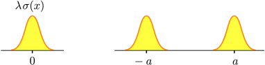
Figure 2: Smooth but sharply peaked backgrounds approximating Dirichlet points: a) one, and b) two at a separation of $2a$. In the “sharp” limit the backgrounds approach delta functions.

The sharp limit is benign in one dimension, so we can take $\sigma(x)$ to be a “spike” $\sigma(x)=\delta(x)$ without difficulty. The renormalized energy of an isolated spike of strength $\lambda$ (see Fig. 2a) is found to be

$$E_{1}(\lambda,m)=\frac{1}{2\pi}\int_{m}^{\infty}dt\frac{t\log\left(1+\frac{\lambda}{2t}\right)-\frac{\lambda}{2}}{\sqrt{t^{2}-m^{2}}}$$ (7)

It is easy to see that this integral converges for any $\lambda$ and $m\neq 0$, but diverges logarithmically as $m\to 0$. Likewise, the renormalized energy of two spikes at $x=\pm a$ is given by,

$$E_{2}(a,\lambda,m)=\frac{1}{2\pi}\int_{m}^{\infty}\!dt\,\frac{t\log\left(1+\frac{\lambda}{t}+\frac{\lambda^{2}}{4t^{2}}(1-e^{-4at})\right)-\lambda}{\sqrt{t^{2}-m^{2}}}$$ (8)

Since these results are central to the rest of the discussion, I’ve appended a derivation (of eq. (7)) at the end of the talk.

Let’s submit these results to the same examination as before: as $a\to\infty$ we find

$$\lim_{a\to\infty}E_{2}(a,\lambda,m)=2E_{1}(\lambda,m)$$ (9)

which is fine; and as $a\to 0$,

$$\lim_{a\to 0}E_{2}(a,\lambda,m)=E_{1}(2\lambda,m)$$ (10)

which is much more satifactory than eq. (5). Also, both $E_{1}$ and $E_{2}$ diverge logarithmically as $m\to 0$, as expected. So the renormalized energy in a sharp background is finite and passes all the tests.

However, the punchline is that both $E_{1}$ and $E_{2}$ diverge like $-\lambda\,\mbox{ln}\,\lambda$ as $\lambda\to\infty$. So the total renormalized Casimir energy diverges as the coupling constant, $\lambda$, is taken strong enough to impose the boundary condition on all modes. $\lambda$ can be regarded as a cutoff, since modes with $\omega\gg\lambda$ are not affected by the interaction. So in this example in a physical material the total, renormalized vacuum fluctuation energy is strongly cutoff dependent. Note that $E_{1}$ and $E_{2}$ are renormalized energies. There are no counterterms available to absorb this divergence.

The two approaches disagree on the total energy, but they agree on the energy density and the force between two points. For any background $\sigma(x)$, the energy density diverges only where $\sigma(x)\neq 0$. For a spike at $a$ the energy density remains finite for $x\neq\pm a$ in the limit $\lambda\to\infty$, and the limiting form agrees with the density calculated using the boundary condition a priori.MT Likewise, the force between the two sharp sources agrees with the boundary condition calculation as $\lambda\to\infty$,

$$\lim_{\lambda\to\infty}-\frac{\partial}{\partial a}E_{2}(a,\lambda,m)=-\frac{\partial}{\partial a}\tilde{E}_{2}(a,m)\ \left(\ =-\frac{\pi}{48a^{2}}\quad\hbox{for}\quad m=0\right)$$ (11)

In fact no measurement of the properties of the two points can detect the infinite energy stored locally on the boundary. This, however, is special to one dimension. Notice also that the vacuum fluctuation energy is negative ($\sim-\lambda\,\mbox{ln}\,\lambda$ as $\lambda\to\infty$). In a more realistic context this energy would be more than overwhelmed by the positive contributions to the energy coming from the curvature of $\sigma$, which goes like $|\sigma^{\prime}|^{2}$, and the potential energy of $\sigma(x)$ which would involve higher powers of $\sigma(x)$ beginning with the mass term $\frac{1}{2}m^{2}\int dx\sigma^{2}(x)$. I left those terms out, not because they aren’t present, but because I was trying to define an abstract problem – the “Dirichlet-Casimir” problem. Having failed, it is clear that the total energy depends not only on the vacuum fluctuation energy of $\phi$, but also on the energy stored in the material represented by $\sigma$. The two cannot be separated – no abstract “Casimir energy” can be defined for the Dirichlet boundary condition in one dimension.

To summarize the results for a scalar field in one dimension:

• The renormalized vacuum fluctuation energy is well defined and finite for any (piecewise continuous) background $\sigma(x)$. It differs from the energy calculated by assuming a boundary condition ab initio. The renormalized energy is material (ie. $\lambda$), dependent, and diverges if $\lambda$ is taken to infinity to impose the boundary condition on all modes.

• The change in the vacuum fluctuation energy with rigid displacement of the boundaries is finite and cutoff independent and can be calculated by imposing the boundary condition ab initio.

3 Physical Effects in Other Dimensions

The result of the previous section would be a merely a curiosity if it could not be measured. In higher dimensions worse divergences occur and they too are always confined to the domain where the background fields are non-zero. Thus in any experiment in which the material ($\equiv$ the background fields) are unchanged, the cutoff dependence will cancel out. A case in point is the standard Casimir force between parallel, grounded, conducting plates. The force is measured by displacing the plates rigidly but not deforming them. The cutoff dependent terms remain unchanged as the plates are moved and the resulting force is finite. The result is the same whether you impose the boundary condition at the beginning or start with a smooth background and impose the boundary condition in a limiting process.

The situation is completely different, however, if the material must be deformed to display the physical effect. The “Casimir pressure” on a sphere is the most interesting example . To measure this it is necessary to compare the total Casimir energy of a sphere of radius $R$ with that of a sphere of radius $R+\delta R$. If there are cutoff dependent terms associated with the material, their contribution to the energy changes as the area changes, and they contribute to the pressure. Thus, calculations of Casimir pressures will differ between the case where boundary conditions are applied ${\it ab\ initio\/}$ and where they are realized as a limit of the coupling to a background field.

To examine these issues quantitatively we have studied the problem of the “Dirichlet sphere” – the boundary condition $\phi(R)=0$ imposed on a massive (or massless) scalar field in $D$ dimensions. $D=2$ is the “Dirichlet circle” and $D=3$ is the sphere. As in the one dimensional example, we replace the boundary condition by the coupling to a non-dynamical scalar background, $\sigma$, with an interaction of the form

$${\mathcal{L}}_{\rm int}=\lambda\sigma(r)\phi^{2}+c_{1}(\epsilon)\sigma+c_{2}(\epsilon)\sigma^{2}+\ldots,$$

where the $\ldots$ denote a finite series of counterterms necessary to renormalized the perturbative divergences generated by the $\phi-\sigma$ interaction. For $D=2$ and $D=3$ only the counterterms shown are needed. We normalized the source so its integral over space is one,

$$\int d^{D}r\sigma(r)=1$$

so the coupling constant, $\lambda$, has dimension $[{\rm mass}]^{2-D}$

We then compute the one-loop effective energy (ie. the Casimir energy), $E_{D}(R,\Delta,\lambda)$, for a background $\sigma$ which is peaked at $r=R$ and has a thickness $\Delta$. We have studied Gaußians and square barriers. The renormalized Casimir energy is finite for fixed $\Delta$, and $\lambda$. However it diverges in the sharp limit, $\Delta\to 0$ (except in one dimension, where we saw that the sharp limit was benign), so that not even the sharp limit exists for $D\geq 2$. If we keep $\Delta$ fixed, and take $\lambda\to\infty$ the Casimir energy diverges as well. The nature of the divergences depends on $D$.

• For the Dirichlet circle ($D=2$), $E_{2}$ diverges like $\frac{\lambda^{2}}{R}\log\Delta$ at fixed $\lambda$ as $\Delta\to 0$. Thus the tension (the two dimensional analog of pressure) diverges logarithmically as the thickness of the “circle” goes to zero.

  This is particularly nicely illustrated by examining the energy density, $\epsilon(r)$, in a spherical shell between $r$ and $r+dr$. The necessary formalism was developed in Ref. Graham:2002xq In Fig. 3a we plot $\epsilon(r)$ for a Gaußian background of fixed strength as a function of its width (denoted $w$ in the figures). As $w\to 0$ the energy density diverges in a non-uniform way: at any fixed $r\neq R$, it approaches a limit. However the closer to $R$, the slower the convergence, and as a result, the total energy diverges as $w\to 0$. The non-uniform behavior is clear in Fig. 3b.

• For the Dirichlet sphere ($D=3$), the leading divergence in $E_{3}$ goes like $\frac{\lambda^{2}}{R^{2}}\frac{\log\Delta}{\Delta}$. Thus the pressure diverges as the thickness of the sphere goes to zero.

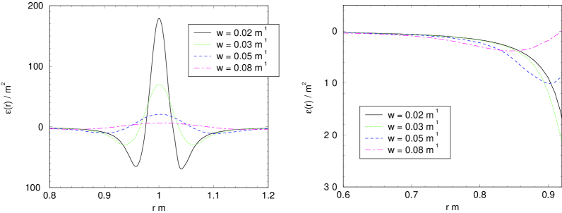
Figure 3: Casimir energy density in a Gaußian background of width $w$ approximating a Dirichlet circle. a) The energy density; b) a closeup of the behavior near $r=0.8/m$.

We expect that these divergences signal that the actual energy depends on the physical properties of the material. $\Delta$ represents its thickness and $\lambda$ plays the role of a frequency cutoff (eg. the plasma frequency, $\omega_{p}$) since modes with $\omega\gg\lambda$ are unaffected by $\sigma$. Since the other stresses to which materials are subject also depend on such properties of the material, we conclude that the Casimir pressure on a surface cannot be defined in a useful way that is independent of the particular dynamical properties of the material.

Since the Casimir energy for any piecewise continuous background, $\sigma$, has an expansion in Feynman diagrams, and since the divergence structure of Feynman diagrams is very well understood, it is interesting to look for the origin of the divergences in the diagrams. The Casimir energy is simply the sum of all one-loop diagrams for $\phi$ circulating in the background $\sigma$. We find that the divergences never come from the loop integrations. Renormalization takes care of those. Instead the divergences come from the integration over the Fourier components of the external lines, $\tilde{\sigma}(p)$. For $D=2$ the divergence comes from the renormalized two-point function. Since the two-point function is easy to calculate, the divergence is easy to display. For $D=3$ the two-point function also generates the leading divergence. However even the three-point function also diverges (logarithmically) for $D=3$. Since the loop integration for the three-point function is manifestly convergent, it provides a very clear demonstration that the divergences as $\Delta\to 0$ cannot be renormalized away by any counterterm available in the continuum theory. Instead they are physical manifestations of the cutoff dependence of the Casimir energy for the Dirichlet sphere.

Our result disagrees with calculations which assume a boundary condition ab initio.Milton:2002vm However those calculations handle divergences in an ad hoc manner and obtain suspicious results: for example the Casimir energy of a Dirichlet sphere is claimed to be finite in odd dimensions ($D=1,3,5,7\ldots$) and to diverge in even dimensions.

The study of field theories in the presence of boundaries is an old subject. The divergences that occur near boundaries have been studied by many authors and with powerful tools.Symanzik:1981wd In particular, it is well known that there are serious divergences near boundaries. Symanzik showed that all the divergences in the presense of boundaries (in certain theories) can be systematically cancelled by the introduction of new counterterms that live on the boundaries. However this begs our question of whether the divergences can be cancelled with only the counterterms available in an underlying interacting quantum field theory without boundaries. As far as I know, the implementation of boundary conditions as a limit of renormalizable, interacting quantum field theories is new.

Although we have only completed our study for the Dirichlet boundary condition, we have examined conducting boundary conditions as well and expect our conclusions to apply to that case as well.

Our interest in vacuum fluctuation energies goes far beyond the question I have discussed today. We are interested in whether quantum fluctuations can generate novel and complex behavior like solitons, in realistic quantum field theories. However, our investigations led us to a close examination of the nature of Casimir effects and to a result surprising enough to be worth telling Joe on the occasion of his birthday!

Appendix

Here is an outline of the calculation of the vacuum fluctuation energy of an isolated “spike”, eq. (7). We start with the universally accepted formula for the sum over zero point energies of a field, $\phi$, fluctuating in a background $\sigma$:

$$E[\sigma]=\frac{1}{2}\sum_{j}\omega_{j}+\frac{1}{2}\int_{0}^{\infty}dk\sqrt{k^{2}+m^{2}}\ \delta\rho(k)$$ (12)

This is just the generalization to the continuum of $\frac{1}{2}\sum\hbar\omega-\hbar\omega_{0}$ (with $\hbar=1$ of course). The $\omega_{j}$ are the energies of possible bound states. $\delta\rho(k)$ is the change in the density of states due to the background $\sigma$. $\delta\rho$ is given by another well known result:

$$\delta\rho(k)=\frac{1}{\pi}\sum_{\ell}\frac{d\delta_{\ell}}{dk}\ ,$$

where $\delta_{\ell}(k)$ is the phase shift for scattering in the $\ell^{\rm th}$ partial wave in the background $\sigma$ (assumed to be symmetric).

$E[\sigma]$ defined by eq. (12) diverges in one dimension. To keep control of divergences we use dimensional regularization: we imagine that we are computing in $D$ dimensions. It can be shown that eq. (12) is finite for $0<D<1$. After isolating the possible divergences and renormalizing we will analytically continue to $D=1$.

Next we use Levinson’s theorem – which equates $\pi$ times the number of bound states to the difference of the phase shift at $k=0$ and $k=\infty$ (valid in $D$ dimensions) to rewrite $E[\sigma]$ as

$$E[\sigma]=\frac{1}{2}\sum_{j}(\omega_{j}-m)+\frac{1}{2\pi}\int_{0}^{\infty}dk(\sqrt{k^{2}+m^{2}}-m)\sum_{\ell}\frac{d\delta_{\ell}}{dk}$$ (13)

At this point it is possible to show that the successive terms in the Born expansion of $\delta_{\ell}$ (the expansion of $\delta$ in powers of $\sigma$) can be put into one-to-one correspondence with the one loop Feynman diagrams. In particular the first Born approximation is identical to the tadpole diagram which diverges as $D\to 1$.

To renormalize, we first subtract the first Born approximation from eq. (13) and add back the tadpole diagram to which it is equal. We then cancel the tadpole diagram against the counterterm $c(\epsilon)$ (see eq. (6)). The resulting renormalized and manifestly finite expression for the Casimir energy can now be evaluated at $D=1$, where the sum over phase shifts includes only the symmetric and antisymmetric channels:

$$E[\sigma]=\frac{1}{2\pi}\int_{0}^{\infty}dk(\sqrt{k^{2}+m^{2}}-m)\frac{d}{dk}\left(\delta_{+}(k)+\delta_{-}(k)-\delta^{(1)}(k)\right)$$ (14)

$\delta^{(1)}(k)$ is the Born approximation to the sum of the phase shifts. To save space I have dropped the sum over bound states since there are none in the case at hand.

Now to the specific case of the $\delta$-function background: The phase shift in the antisymmetric channel vanishes. The symmetric channel phase shift is easily computed:

$$\delta_{+}(k)=\tan^{-1}\frac{\lambda}{2k}$$

and the first Born approximation is

$$\delta^{(1)}(k)=\frac{\lambda}{2k}$$

The resulting integral,

$$E(\lambda,m)=\frac{\lambda^{3}}{4\pi}\int_{0}^{\infty}dk\frac{\sqrt{k^{2}+m^{2}}-m}{k^{2}(\lambda^{2}+4k^{2})}$$

is most easily evaluated by rotating the contour to the positive imaginary axis and integrating by parts. The result is the expression quoted in eq. (7).

References

- (1) N. Graham, R. L. Jaffe, V. Khemani, M. Quandt, M. Scandurra and H. Weigel, arXiv:hep-th/0207205.
- (2) N. Graham, R. L. Jaffe, V. Khemani, M. Quandt, O. Schröder, and H. Weigel, in preparation.
- (3) V.M. Mostepanenko and N.N. Trunov, The Casimir Effect and its Application, Clarendon Press, Oxford (1997), K. A. Milton, The Casimir Effect: Physical Manifestations Of Zero-Point Energy, World Scientific (2001). M. Bordag, U. Mohideen and V. M. Mostepanenko, Phys. Rept. 353, 1 (2001) [arXiv:quant-ph/0106045].
- (4) N. Graham, R. L. Jaffe, V. Khemani, M. Quandt, M. Scandurra and H. Weigel, Nucl. Phys. B 645, 49 (2002) [arXiv:hep-th/0207120].
- (5) N. Graham, R. L. Jaffe and H. Weigel, Int. J. Mod. Phys. A 17, 846 (2002) [arXiv:hep-th/0201148].
- (6) K. A. Milton, arXiv:hep-th/0210081.
- (7) K. Symanzik, Nucl. Phys. B 190, 1 (1981). P. Candelas, Annals Phys. 143, 241 (1982). D. Deutsch and P. Candelas, Phys. Rev. D 20, 3063 (1979). G. Barton, Rept. Prog. Phys. 42, 963 (1979).