Abstract

We study the propagating gravitational waves as a tool to probe the extra dimensions. In the set-up with one compact extra dimension and non-gravitational physics resigning on the 4-dimensional subspace (brane) of 5-dimensional spacetime we find the Green’s function describing the propagation of 5-dimensional signal along the brane. The Green’s function has a form of the sum of contributions from large number of images due to the compactness of the fifth dimension. Additionally, a peculiar feature of the causal wave propagation in five dimensions (making a five-dimensional spacetime very much different from the familiar four-dimensional case) is that the entire region inside the past light-cone contributes to the signal at the observation point. The 4-dimensional propagation law is nevertheless reproduced at large (compared to the size of extra dimension) intervals from the source as a superposition of signals from large number of images. The fifth dimension however shows up in the form of corrections to the purely 4-dimensional picture. We find three interesting effects: a tail effect for a signal of finite duration, screening at the forefront of this signal and a frequency-dependent amplification for a periodic signal. We discuss implications of these effects in the gravitational wave astronomy and estimate the sensitivity of gravitational antenna needed for detecting the extra dimension.

1. Introduction

Over decades since the works of Kaluza and Klein the idea of extra dimensions enjoys constantly growing interest of the physical community. Designed originally to serve the unification of the General Relativity and Maxwell electrodynamics it is now more fashionable to invoke the extra dimensions for solving the problems of hierarchy and vacuum energy. A recent review on old and new paths to the extra dimensions is [1]. It is customary nowadays to consider the Kaluza-Klein idea in the context of the brane paradigm. According to this picture, the non-gravitational physics, conveniently described by the Standard Model, is confined to a $(3+1)$-dimensional subspace called brane of the $(4+n)$-dimensional space-time with $n$ compactified extra dimensions. Only gravitational field is allowed to propagate through the whole spacetime and probe the extra dimensions. If $L$ is a typical size of the extra dimensions the gravitational physics on the brane is expected to be $(4+n)$-dimensional on the scales of order $L$ and smaller while the familiar 4-dimensional gravitational interaction is supposed to emerge on the much larger than $L$ scales. A standard way to study this is to look at the static Newton potential along the brane. At large distances $r\gg L$ it takes the 4-dimensional form $G_{4}/4\pi r$, with $G_{4}$ being the induced 4-dimensional Newton constant, while the higher dimensional physics manifests in exponentially small corrections, $e^{-r/L}$.

In this paper we give up staticity and look at propagation of waves. The higher-dimensional corrections to the purely 4-dimensional law of propagation then are no more exponentially small but have a power law. This makes the waves a more convenient tool for probing the extra dimensions. Some puzzling surprises are however awaiting for us on this venue. Most surprising is the fact that the causal propagation of wave signals from a source is radically different for odd and even dimensions. This difference is most transparent in the retarded potentials. In even dimensions, $(3+1)$-dimensional space-time being a particular example, the retarded potential is proportional to the delta-function of $(t-r)$ and thus is concentrated on the future light-cone and vanishing everywhere else. In contrast, the retarded potential in odd spacetime dimensions has support everywhere inside the light-cone! Additionally, there appear non-integrable divergences on the forefront of the propagating wave. The above properties make the wave propagation in 5-dimensional space-time very much different from the propagation in the 4-dimensional case. In particular, the night sky would look quite differently if we lived in 5-dimensional Universe. Even already dead stars would still produce flashing spots on the sky so that night would not be as dark as in our home Universe. A natural question arises: how after all these differences the large scale propagation on the brane still manages to be 4-dimensional even though it is built out of the 5-dimensionally propagating waves. In this paper we address this question and moreover study the manifestations of the 5-dimensional character of the wave propagation in the form of corrections to the purely 4-dimensional law.

We find a few interesting effects. First, we consider propagation of a signal of finite duration $T$ emitted by a source on the brane. In purely 4-dimensional picture an observer at some large distance from the source would see a pulse of same finite duration $T$. In the 5-dimensional picture with compact extra dimension the signal detected by an observer is a superposition of signals coming from large number of images additionally to the original source. In fact, the purely 4-dimensional picture arises as a result of this superposition. The corrections are however important. Most significantly, when the entire signal has passed through the point of observation there still remain signals coming from the images which are inside the past light-cone of the point of observation. These signals keep arriving and result in a tail, a power-like decaying with time signal. The whole effects thus is due to the combination of the 5-dimensional feature of the propagation inside the light-cone which we mentioned above and the compactness of the fifth dimension manifested in presence of large number of images. On the other hand, the shape of the forefront of the signal is modified by what we call screening effect: corrections appear with negative sign and smooth out the otherwise a step-like forefront profile. Another effect appears for the periodic signal. We find that the amplitude of the signal at the point of observation is amplified with a frequency-dependent amplification factor. Both effects are proportional to $L$ in some power and are clear indications of the presence of the extra dimension. This makes it interesting to reconcile these effects with modern observational possibilities available at LIGO or LISA.

This paper is organized as follows. In section 2 we formulate the set-up and find various representations for the Green’s function describing propagation of the 5-dimensional signal along the lower-dimensional subspace (brane). We focus on the retarded potentials in section 3 and derive the 5-dimensional potential consistent with the boundary conditions we impose along the fifth dimension. The propagation of the finite pulse is considered in section 4 and the periodic signal in section 5. In section 6 we estimate the predicted effects and compare them with the available sensitivity of the gravitational detectors.

2. Many faces of the Green’s function

2.1. The set-up

We consider flat 5-dimensional space-time covered by coordinates $X^{A}=(x^{\mu},y)$ where $y$ is the coordinate along the fifth dimension and $x^{\mu},~{}\mu=0,1,2,3$ are the four-dimensional coordinates. We restrict the coordinate $y$ to lie within the interval between $y=0$ and $y=L$ and we impose the Neumann boundary conditions on the perturbations of the five-dimensional gravitational field at the ends of this interval. $L$ is thus a size of the extra dimension. Our four-dimensional world with experimental devices, standard model particles and human beings resign on the four-dimensional subspace at $y=0$ so that only gravitational field may propagate into the fifth dimension. The subspace $y=0$ (as well as the one at $y=L$) can be also thought of as a zero-tension brane. We sometimes will use this terminology. A generalization to branes with non-vanishing tension (the Neumann boundary condition then has to be replaced by a condition of the Robin type) is possible although technically more involved. Another possible setting is to impose the periodic boundary conditions $\phi(x,y=0)=\phi(x,y=L)$, where $\phi(x,y)$ stands for the relevant five-dimensional perturbation. In this case we have a standard Kaluza-Klein configuration. Although all our results are naturally extended to the case with periodic boundary conditions, we will stick to the scenario with the Neumann boundary conditions.

2.2. Kaluza-Klein representation

It should be noted that in what follows we systematically ignore the tensor structure of the gravitational perturbations assuming that the field equation of interest takes the form of the scalar type field equation

$$\left(-\partial_{0}^{2}+\partial_{y}^{2}+\partial_{{\bf x}}^{2}\right)\phi(y,x^{0},{\bf x})=0~{}~{}$$ (2.1)

subject to the boundary conditions

$$\partial_{y}\phi(y,x^{0},{\bf x})|_{y=0}=\partial_{y}\phi(y,x^{0},{\bf x})|_{y=L}=0~{}~{}.$$ (2.2)

The normalized modes forming the basis of functions in the $y$-direction are

$$\varphi_{n}(y)=\frac{1}{\sqrt{L}},\,\,\,n=0$$ (2.3)

$$\varphi_{n}(y)=\sqrt{\frac{2}{L}}\,\cos(m_{n}\,y),\,\,\,\,m_{n}=\frac{n\pi}{L}~{}~{},\,\,\,n>0$$ (2.4)

while in the $x$-direction the modes are the usual plane waves $e^{ipx}$ appropriately normalized on the delta-function. In terms of these modes the 5-dimensional propagator (or the Green’s function) defined as a solution to the field equation with delta-like source

$$-\nabla^{2}_{5}~{}D_{5}(X,X^{\prime})=\delta(X,X^{\prime})$$ (2.5)

takes the following five-dimensional momentum space representation

$$D_{5}(X,X^{\prime})=\frac{1}{(2\pi)^{4}}\int d^{4}p\,\sum\limits_{n=0}^{\infty}e^{ip(x-x^{\prime})}\;\frac{\varphi_{n}(y)\,\varphi_{n}(y^{\prime})}{p^{2}+m^{2}_{n}}~{}~{},$$ (2.6)

where $p^{2}=-p_{0}^{2}+{\bf p}^{2}$. In Lorentzian signature there are various types of propagator depending on the contour chosen when the integration over momenta is taken. The particular choices of the integration will be discussed in the next section. Here for simplicity of the presentation we switch to the Euclidean signature by means of the analytic continuation $p_{0}=ip_{4}$ so that $p^{2}$ becomes a positive quantity and the problem of the integration contour does not arise.

We see that $m_{n}$ introduced in (2.4) have the meaning of the Kaluza-Klein masses. Note that in case of periodic boundary conditions we would get a similar form for the propagator with different set of Kaluza-Klein masses $m_{n}=2\pi n/L$.

The main object of interest in the present paper is the reduction of the propagator (2.6) to the subspace $y=0$. In other words, we are interested in the situation when the gravitational 5-dimensional signal propagates between two points on the subspace where we happen to live. This propagation is described by the quantity

$$D(x,x^{\prime})\equiv\left.D_{5}(X,X^{\prime})\,\right|_{y=y^{\prime}=0}~{}~{}.$$ (2.7)

It is clear from equation (2.6) that $D(x,x^{\prime})$ reduces to the series of 4-dimensional massive Green’s functions of the Kaluza-Klein tower

$$D(x,x^{\prime})=\frac{1}{(2\pi)^{4}L}\int d^{4}p\,\sum\limits_{n=-\infty}^{\infty}\frac{e^{ip(x-x^{\prime})}}{p^{2}+m^{2}_{n}}=\frac{1}{L}\sum\limits_{n=-\infty}^{\infty}D(m_{n}^{2}|\,x-x^{\prime})~{}~{},$$ (2.8)

where

$$D(m^{2}|\,x-x^{\prime})=\frac{m}{4\pi^{2}}\frac{K_{1}(m|x-x^{\prime}|)}{|x-x^{\prime}|},\,\,\,\,|x-x^{\prime}|=\sqrt{(x-x^{\prime})^{2}}$$ (2.9)

is the 4-dimensional propagator of massive field given in Euclidean space by the MacDonald function of the first order. Equation (2.8) gives us the first, very natural from the Kaluza-Klein perspective, representation for the brane-to-brane propagator as mediated by the set of massive Kaluza-Klein fields.

2.3. Momentum space representation

Another way to look at the expression (2.8) is to consider it as a momentum space representation for the entirely four-dimensional propagator

$$D(x,x^{\prime})=\frac{1}{(2\pi)^{4}L}\int d^{4}p\,D(p)\,e^{ip(x-x^{\prime})}$$ (2.10)

with the non-trivial propagator $D(p)$ as a function of the 4-dimensional momentum $p$. $D(p)$ is expressed in terms of the infinite sum over Kaluza-Klein masses as in (2.8). For the tower of these masses given by (2.4) (tracing back to the boundary conditions (2.2)) the sum over $n$ can be calculated explicitly and the answer is

$$D(p)\equiv\sum\limits_{n=-\infty}^{\infty}\frac{1}{p^{2}+m^{2}_{n}}=\frac{L}{p}\frac{\cosh(Lp)}{\sinh(Lp)},\,\,\,p=\sqrt{p^{2}}~{}~{}.$$ (2.11)

Notice that (2.11) is valid for the Euclidean signature. Switching to the Lorentzian signature is provided by the analytic continuation $p\rightarrow ip$ so that the Lorentzian form of the propagator $D(p)$ at timelike momenta is the following

$$D_{M}(p)={L\over p}{\cos(Lp)\over\sin(Lp)},\,\,\,p=\sqrt{-p^{2}}~{}~{}.$$ (2.12)

Notice that it has poles at real values of $p$, $L\,p=\pi\,n$, which correspond to the Kaluza-Klein modes. Additionally $D_{M}(p)$ has zeros at $Lp={\pi\over 2}(2n+1)$, $n$ is integer. The physical interpretation of the zeros of the propagator is less clear. At large values of momentum (or, respectively for very short space-time intervals) the propagator (2.11) behaves as $D(p)\sim{1\over p}$, the typical behavior of truly 5-dimensional propagation as it is seen from a lower-dimensional subspace. On the other hand, at small values of momentum (i.e. at large intervals on the brane) the four-dimensional behavior $D(p)\sim{1\over p^{2}}$ is recovered. This guarantees us that the four-dimensional physics is reproduced at large scales even though the underlying physics is 5-dimensional. The cross-over between two regimes happens at the space-time intervals $s^{2}(x,x^{\prime})$ of order $L^{2}$. Provided we were not aware that our four-dimensional world is embedded into a higher-dimensional space-time we would have to deal with the propagator (2.12) as a non-trivial function of the 4-momentum $p$ not being aware about its Kaluza-Klein origin.

2.4. Sum over images representation

The integration over momentum in (2.10) includes the integration over angles and the integration over absolute value $p$ of the 4-momentum. Inserting the exact expression (2.11) into (2.10) the integration over angles can be performed explicitly and gives

$$D(x)=\frac{1}{4\pi^{2}}\frac{1}{|x|}\int\limits_{0}^{\infty}dp\,p\,{1\over L}\,D(p)\,J_{1}(p|x|)~{}~{},$$ (2.13)

where the table integral

$$\int\limits_{0}^{\pi}d\theta\,\sin^{2}\theta\,e^{iy\cos\theta}=\frac{\pi}{y}\,J_{1}(y)$$ (2.14)

has been used. Taking into account that on the real axis the following relation holds between the Bessel and Hankel functions

$$J_{1}(z)=\frac{1}{2}\left(H^{(1)}_{1}(z)+H^{(2)}_{1}(z)\right)=\frac{1}{2}\left(H^{(1)}_{1}(z)+H^{(1)}_{1}(-z)\right)$$ (2.15)

one can transform the integral to the integration over the whole real axis of $p$ with the principal value prescription at $p=0$

$$\int\limits_{0}^{\infty}dp\,p\,{1\over L}\,D(p)\,J_{1}(p|x|)=\frac{1}{2}\,{\rm P}\int\limits_{-\infty}^{\infty}dp\,p\,{1\over L}\,D(p)\,H^{(1)}_{1}(p|x|)~{}~{}.$$ (2.16)

By closing the contour of integration in the upper-half plane of the complex variable $p$ one finds that the result reduces to the contribution of poles on the imaginary semiaxis, $p_{n}=im_{n}$, $n\geq 0$ (the pole at $n=0$ contributing only one half of the residue in view of the principal value integration above)

$$\int\limits_{0}^{\infty}dp\,p\,\frac{\cosh(Lp)}{\sinh(Lp)}\,J_{1}(p|x|)=\frac{1}{L|x|}+\frac{2\pi}{L^{2}}\,\sum\limits_{n=1}^{\infty}n\,K_{1}(m_{n}|x|)~{}~{},$$ (2.17)

where $K_{1}(z)=-\pi H^{(1)}_{1}(iz)$ is the modified Bessel (MacDonald) function. In view of the relation $K_{1}(z)=-\partial_{z}K_{0}(z)$ between the MacDonald functions of the zeroth and first order, one has

$$\int\limits_{0}^{\infty}dp\,p\,\frac{\cosh(Lp)}{\sinh(Lp)}\,J_{1}(p|x|)=\frac{1}{L|x|}-\frac{2\pi}{L^{2}}\,\partial_{z}\!\sum\limits_{n=1}^{\infty}K_{0}(nz)\,\Big{|}_{z=\pi|x|/L}~{}~{},$$ (2.18)

where the series of McDonald functions can be calculated with the aid of the formula [8]

$$\sum\limits_{n=1}^{\infty}K_{0}(nz)=\frac{1}{2}\left({\mathbf{C}}+\ln\frac{z}{2\pi}\right)+\frac{\pi}{2z}+\pi\sum\limits_{n=1}^{\infty}\left(\frac{1}{\sqrt{z^{2}+4\pi^{2}n^{2}}}-\frac{1}{2\pi n}\right)~{}~{}.$$ (2.19)

Putting things together this gives us yet another, coordinate space, representation for the propagator

$$D(x,x^{\prime})=\frac{1}{4\pi^{2}}\sum\limits_{n=-\infty}^{\infty}\frac{1}{((x-x^{\prime})^{2}+4n^{2}\,L^{2})^{3/2}}~{}~{}.$$ (2.20)

This result obviously reproduces the recovery of the Green’s function along the brane by another method – method of images. Indeed, it can be obtained by summing the contributions of images of the original source, located at the infinite sequence of points $X_{n}$

$$D(x)=2\sum\limits_{n=-\infty}^{\infty}D_{5}(X-X_{n})\,\Big{|}_{\,X=(x,0)},$$ (2.21)

$$X_{n}=(0,\,2nL),\,\,\,\,(X-X_{n})^{2}=x^{2}+4n^{2}L^{2}~{}~{},$$ (2.22)

mediated by the five-dimensional Green’s function

$$D_{5}(X,X^{\prime})=\frac{1}{8\pi^{2}}\frac{1}{((X-X^{\prime})^{2})^{3/2}}~{}~{}.$$ (2.23)

The representation (2.20) of the propagator expresses the obvious fact that there many ways to propagate signal between two space-time points on the brane: it may propagate entirely along the brane (the $n=0$ term in the sum (2.20)) or through the fifth dimension reflecting off the second brane at $y=0$ and coming back to our brane. Each such propagation contributes to the sum in (2.20). Since the number of reflections can be arbitrary high the sum has infinite number of terms.

When $(x-x^{\prime})^{2}$ is much larger than $L^{2}$ the sum in (2.22) can be approximated by the integral, $\sum_{n}={1\over 2L}\int\,dy$ where $y=2\,L\,n$. Evaluating the integral we find

$$D(x,x^{\prime})\simeq{1\over 8\pi^{2}L}\int_{-\infty}^{+\infty}dy\,{1\over((x-x^{\prime})^{2}+y^{2})^{3/2}}={1\over 4\pi^{2}L}\,{1\over(x-x^{\prime})^{2}},$$ (2.24)

so that 4-dimensional Green’s function is recovered in this limit. It is actually a realization of the well-known in mathematics method called descent method to obtain Green’s function from a Green’s function one dimension higher. Thus, the 4-dimensional propagator is recovered for large (compared to $L$) intervals on the brane as a result of superposition of contributions from infinite number of images.

2.5. Newton potential

We finish this section with a brief illustration of how the Newton potential emerges from our analysis. Indeed, the Newtonian potential on the brane can be easily recovered from (2.20) by integrating over time (it is again a realization of the descent method discussed in the previous subsection)

$$V(r)=\int\limits_{-\infty}^{\infty}dx^{4}\,D({\mathbf{x}},x^{4})=\frac{1}{2\pi^{2}}\sum\limits_{n=-\infty}^{\infty}\frac{1}{r^{2}+4n^{2}L^{2}}~{}~{},~{}~{}r^{2}={\bf x}^{2}~{}~{}.$$ (2.25)

In view of the summation formula (2.11) it equals

$$V(r)=\frac{1}{4\pi r}\left(1+\frac{2}{e^{\pi r/L}-1}\right)$$ (2.26)

and, thus, reproduces at large distances $r\gg L$ the usual four-dimensional Newtonian potential with Yukawa-type corrections in the four-dimensional world. For small distances $r\ll L$ it obviously features the five-dimensional behavior $\sim 1/r^{2}$.

3. Retarded potentials

The retarded Green’s function which is an object of our prime interest here can be obtained from the Euclidean Green’s functions of the previous section by the analytic continuation. This can be done directly in the final result (2.20) in the coordinate representation, or separately for massive Green’s functions of the Kaluza-Klein tower in (2.8). Here we choose the first method, and its equivalence to the second one is shown in the Appendix A.

To distinguish the coordinates of the Lorentzian spacetime $x=(x^{0},{\mathbf{x}})$ from those of the Euclidean space we supply the latter by the subscript $E$, $x_{E}=(x^{4},{\mathbf{x}})$. They are related by the Wick rotation

$$x_{E}\equiv(x^{4},{\mathbf{x}})=(ix^{0},\,{\mathbf{x}}),$$ (3.1)

$$x_{E}^{2}\equiv(x^{4})^{2}+{\mathbf{x}}^{2}=-(x^{0})^{2}+{\mathbf{x}}^{2}+i\varepsilon=x^{2}+i\varepsilon~{}~{},$$ (3.2)

which in particular determines the analytic continuation from the (massive) Euclidean Green’s function

$$(m^{2}-\nabla^{2}_{E})D_{E}(x_{E})=\delta(x_{E})$$ (3.3)

to the Feynman propagator in Lorentzian spacetime – the boundary value on the real axis of the Lorentzian spacetime interval $x^{2}$ when approaching from the upper half complex plane of $x^{2}$ according to (3.2), $\varepsilon\to 0$, [9]

$$(m^{2}-i\varepsilon-\nabla^{2})D_{F}(x)=\delta(x)~{}~{},~{}~{}D_{F}(x)=iD_{E}(x_{E})\,\Big{|}_{\,x_{E}=(ix^{0},\,{\mathbf{x}})}$$ (3.4)

(the factor $i$ here follows from the formal identification $\delta(x)=i\delta(x_{E})$ matching with (3.1)).

As is well known [9], other Green’s functions in flat spacetime can be obtained from the Feynman propagator by taking its real and imaginary parts and multiplying it with distributions reflecting the needed causality properties. In particular, the retarded propagator reads

$$D_{R}(x)=2\,\theta(x^{0})\,{\rm Re}\,D_{F}(x)~{}~{}.$$ (3.5)

We illustrate this prescription for massless field propagator. Starting with the massless Euclidean Green’s function in four-dimensions

$$D_{E}(x_{E})\Big{|}_{\,m^{2}=0}=\frac{1}{4\pi^{2}}\frac{1}{x_{E}^{2}}$$ (3.6)

one finds in view of (3.3) and (3.5) the well-known retarded Green’s function of a massless field

$$D_{R}(x)\Big{|}_{\,m^{2}=0}=\frac{\theta(x^{0})}{2\pi^{2}}\,{\rm Re}\frac{i}{x^{2}+i\varepsilon}=\frac{\theta(t)}{4\pi}\frac{\delta(r-t)}{r},\,\,\,r=|{\mathbf{x}}|~{}~{},\,\,\,t=x^{0}~{}~{},$$ (3.7)

where in the last line the well-known formula

$${1\over x^{2}+i\varepsilon}-{1\over x^{2}-i\varepsilon}=-2\pi i\delta(x^{2})$$

has been used. Important feature of this propagator in four dimensions is that it has a support on the past light cone of the observation point. As we shall see in a moment the behavior of the retarded potential in five dimensions is rather different.

Application of this rule to 5-dimensional Green’s function (2.23) or (2.20) is trickier because of the branching points in this expression. Wick rotation for the Euclidean Green’s function (2.20) is based on the relation

$$(x^{2}\pm i\varepsilon)^{\lambda}=|x^{2}|^{\lambda}\,e^{\pm i\pi\lambda\theta(-x^{2})}~{}~{},\,\,\,\,|\lambda|<1~{}~{}.$$ (3.8)

Because of the restriction on $\lambda$ we cannot apply the above formula immediately to (2.23) in which $\lambda=3/2$. Therefore, we first effectively lower the degree of the singularity by noting that

$$\frac{1}{(x^{2}+i\varepsilon)^{3/2}}=-\frac{1}{r}\,\frac{\partial}{\partial r}\frac{1}{(r^{2}-t^{2}+i\varepsilon)^{1/2}}~{}~{}$$ (3.9)

and then apply (3.8) to get

$$D_{R}^{(5)}(r,t)={1\over 4\pi^{2}}{\rm Re}\,\frac{i}{(r^{2}-t^{2}+i\varepsilon)^{3/2}}=-{1\over 4\pi^{2}r}\,\frac{\partial}{\partial r}\frac{\theta(t-r)}{(t^{2}-r^{2})^{1/2}}~{}~{}.$$ (3.10)

We should apply now this formula to each term in (2.20) so that finally the kernel of the retarded Green’s function takes the form

$$D_{R}(t,{\mathbf{x}})=-\frac{1}{2\pi^{2}}\!\sum\limits_{n=-\infty}^{\infty}\frac{1}{r}\,\frac{\partial}{\partial r}\,\frac{\theta(t-\sqrt{r^{2}+4n^{2}L^{2}})}{\sqrt{t^{2}-r^{2}-4n^{2}L^{2}}}~{}~{}.$$ (3.11)

An alternative derivation of this result, starting directly with retarded propagators for massive Kaluza-Klein modes in (2.8), is given in the Appendix A. Two drastic differences from the 4-dimensional case (3.7) should be mentioned. First, the retarded Green’s function (3.10), (3.11) has support on entire region inside the future light-cone (in 4-dimensional case the support was just on the surface of the light-cone) of the delta-like source at $r=0,\ t=0$. Second, the presence of non-integrable singularity on the light-cone in (3.10) should be noted. Additionally, all images of the original source, belonging to the interior of the past light cone of the observation point, contribute to the Green’s function (3.11).

4. Finite pulse

The brane-to–brane Green’s function (3.11) gives on the brane $y=0$ the solution of the equation

$$\nabla^{2}_{5}\Phi(X)=-G_{5}\,J(X)$$ (4.1)

with zero initial conditions in the past and with the source $J(X)$ located on the same brane

$$J(x,y)=\,f(t)\,\delta^{(3)}({\mathbf{x}})\,\delta(y)~{}~{}.$$ (4.2)

Here $G_{5}$ denotes the five-dimensional gravitational coupling constant. This solution reads

$$\Phi(t,{\mathbf{x}})=G_{5}\int\limits_{-\infty}^{\infty}dt^{\prime}\,D_{R}(t-t^{\prime},{\mathbf{x}})\,f(t^{\prime})~{}~{}.$$ (4.3)

Substituting (3.11) we have

$$\Phi(t,{\mathbf{x}})=-\frac{G_{5}}{2\pi^{2}}\sum\limits_{n=-\infty}^{\infty}\frac{1}{r_{n}}\,\frac{\partial}{\partial r_{n}}\int\limits_{-\infty}^{t-r_{n}}dt^{\prime}\,\left.\frac{f(t^{\prime})}{\sqrt{(t-t^{\prime})^{2}-r_{n}^{2}}}\,\right|_{\,r_{n}=(r^{2}+4n^{2}L^{2})^{1/2}}~{}~{}.$$ (4.4)

When the source $f(t)$ in (4.2) has the form of a constant pulse of a finite duration $T$,

$$f(t)=\theta(t)-\theta(t-T)~{}~{},$$ (4.5)

the expression (4.4) (after the integration over $t^{\prime}$ has been performed) takes the form

$$\Phi(t,{\mathbf{x}})=\frac{G_{5}}{16\pi^{2}L^{3}}\,t\,\theta(t-r)\,I\left(\alpha,\beta\,|\,[\alpha]\right)-(t\to t-T)~{}~{},$$ (4.6)

in terms of the function $I(\alpha,\beta\,|\,[\alpha])$ of the two parameters

$$\alpha=\frac{\sqrt{t^{2}-r^{2}}}{2L}~{}~{},$$ (4.7)

$$\beta=\frac{r}{2L}~{}~{}.$$ (4.8)

Here the square brackets in the notation $[\alpha]$ denote the integer part of $\alpha>0$ and the function of three arguments $I(\alpha,\beta\,|\,m)$ is given by the following finite sum

$$I(\alpha,\beta\,|\,m)=\sum\limits_{n=-m}^{m}\frac{1}{(\beta^{2}+n^{2})\sqrt{\alpha^{2}-n^{2}}}~{}~{},\,\,\,\,m<\alpha~{}~{}.$$ (4.9)

Let us first discuss the contribution of the forefront of the pulse – the first term of (4.5). With $t$ reaching the value of the radial coordinate $r$ at which the observer is located, the observer starts getting the signal encoded in the first term of (4.6). As long as this term depends on the integer part of the parameter $\alpha$, $m=[\alpha]$, this signal is not continuous in time. For any value of time when $\alpha$ becomes integer, a new pair of terms at $n=\pm[\alpha]$ appear in the sum (4.9) and the value of the sum changes discontinuously. This corresponds to the fact that the signals from the two new images located at $y=\pm 2[\alpha]L$ reach the observer. Moreover, immediately at $\alpha=[\alpha]$ these signals are singular, because they are proportional to $1/\sqrt{\alpha-[\alpha]}$. This is a direct consequence of the structure of singularity of the retarded Green’s function in five dimensions. In contrast to four dimensions its support is not restricted to the past light cone, rather it is given by the entire interior of the latter (see Eq.(3.10)), and the Green’s function kernel in (3.10) has a singularity $\sim 1/(t^{2}-r^{2})^{3/2}$ at $t\to r+0$. Because of the square root the corresponding singularity in the $m=\pm[\alpha]$ terms of (4.9) is not strong, and when averaged over the time lapse between two consequitive singularities gives, as we show below, a finite contribution.

Immediately after $t$ reaches the value of $r$ only the zeroth term of the sum (4.9), $1/\alpha\beta^{2}=8L^{3}/r^{2}\sqrt{t^{2}-r^{2}}$ contributes to the signal (4.6). This corresponds to the contribution of only the source located at $y=0$ (and its image merging with the source and, thus, doubling its value – see discussion in Sect.2). Therefore this contribution is essentially 5-dimensional by its nature and reflects the fact that the retarded potential (3.10) in five dimensions has non-integrable singularity on the lightcone. As time goes on more signals from images start to arrive so that at sufficiently large time the signal detected on the brane has the shape of a sequence of singular spikes. Obviously, an observer on the brane with devices at hand is not capable to resolve the spikes so that the time averaging which we employ below in the paper becomes a meaningful procedure.

The recovery of the 4-dimensional nature of the signal for a given $r$ takes place after some time when the signals from many images reach the observer and form the cumulative effect of many terms in the sum (4.9). This situation corresponds to the limit of $\alpha\gg 1$. The calculation of the sum (4.9) in this limit is presented in the Appendix B and gives the following result in the first two orders of the asymptotic $1/\alpha$-expansion

$$I(\alpha,\beta\,|\,[\alpha])=\frac{\pi}{\beta}\,\frac{\coth\pi\beta}{\sqrt{\alpha^{2}+\beta^{2}}}-\frac{2^{3/2}}{\alpha^{2}+\beta^{2}}\,\sqrt{\frac{\delta}{\alpha}}\,\left[\,1-\frac{1}{\sqrt{2}}\,I(\delta)\,\right]_{\,\delta=\alpha-[\alpha]+1}$$

$$\qquad\qquad+\frac{2^{1/2}}{\alpha^{2}+\beta^{2}}\,\frac{1}{\sqrt{\alpha(\alpha-[\alpha])}}+{\rm O}\left(\frac{1}{\alpha^{7/2}}\right)~{}~{}.$$ (4.10)

Here $I(\delta)$ is the following integral of the parameter $\delta=\alpha-[\alpha]+1$ belonging the finite range $1\leq\delta<2$

$$I(\delta)=\int\limits_{0}^{\infty}\frac{dy}{e^{2\pi y\delta}-1}\,\left(\frac{(1+y^{2})^{1/2}-1}{1+y^{2}}\right)^{1/2}.$$ (4.11)

This integral is a decreasing function bounded in this range by its very small value at $\delta=1$, $I(1)\simeq 0.03$ and in what follows gives a negligible contribution.

Similarly to the situation with small $\alpha$, the last term of (4.10) becomes singular also at large integer values of $\alpha$, which corresponds to the arrival of the signal from the new distant pair of images located at $|y|=2[\alpha]L\sim t\gg L$. Interestingly, though, that the singular spikes occurring for late times with the period $\Delta t\simeq 4(\alpha L^{2}/t)\Delta\alpha=2L\sqrt{1-r^{2}/t^{2}}\to 2L$ have now integrable singularities, so that the averaging over time of this spiky signal gives a finite average value. This averaging obviously implies that the temporal resolution threshold of the observing device is much bigger than the period $2L$ of spikes for hypothetic values of $L$ belonging to a millimetre range.

Thus, the temporal averaging of the spike singularity in (4.10) is finite and equals

$$\Big{<}\Big{(}\alpha-[\alpha]\Big{)}^{-1/2}\Big{>}\equiv\int\limits_{[\alpha]}^{[\alpha]+1}\frac{d\alpha}{\sqrt{\alpha-[\alpha]}}=2$$ (4.12)

(we are averaging here only the most rapidly varying singular factor while the other factors for $\alpha\gg 1$ can be regarded nearly constant). Similarly in the second term of (4.10) the averaging gives

$$\Big{<}\sqrt{\alpha-[\alpha]+1}\Big{>}\equiv\int\limits_{[\alpha]}^{[\alpha]+1}d\alpha\,\sqrt{\alpha-[\alpha]+1}=\frac{2}{3}\,\Big{(}2^{3/2}-1\Big{)}~{}~{}.$$ (4.13)

Assembling these results together and taking into account the smallness of $I(\delta)<0.03$ in (4.10), one has the dominant contribution to the temporal average of $I(\alpha,\beta\,|\,[\alpha])$

$$\Big{<}I(\alpha,\beta\,|\,[\alpha])\Big{>}=\frac{\pi}{\beta}\,\frac{\coth\pi\beta}{\sqrt{\alpha^{2}+\beta^{2}}}+\frac{2^{3/2}}{\sqrt{\alpha}(\alpha^{2}+\beta^{2})}\,\frac{5-2^{5/2}}{3}~{}~{},\,\,\,\,\,\,\,\alpha\gg 1$$ (4.14)

Substituting this expression to (4.6) and taking into account the values of parameters (4.7)-(4.8) we finally have the retarded potential averaged over the time lapse between singular spikes

$$\Big{<}\Phi(t,{\mathbf{x}})\Big{>}=\frac{G_{4}}{4\pi r}\,\left(1+\frac{2}{e^{\pi r/L}-1}\right)\,\theta(t-r)$$

$$\qquad-\frac{G_{4}}{3\pi^{2}t}\,\left(\frac{L^{2}}{t^{2}-r^{2}}\right)^{1/4}(2^{5/2}-5)\,\theta(t-r)$$

$$\qquad-(t\to t-T)~{}~{},\,\,\,\,\,\,\,\,\,\,t^{2}-r^{2}\gg L^{2}~{}~{}.$$ (4.15)

Here $G_{4}$ is an effective 4-dimensional gravitational constant

$$G_{4}=\frac{G_{5}}{L}$$ (4.16)

and the subtracted term at $t-T$ gives the contribution of the back front of the pulse (4.5) of finite duration $T$. It should be noted that the first term in (4.15) is exactly the signal expected in 4-dimensions. Remarkably, the radial function there is exactly the Newton potential which we calculated in section 2. The second term in (4.15) is a correction which originated entirely due to the contribution of signals arriving at a given point from large number of images.

When $t>T+r$ both signals from the forefront and the backfront (as well as from their images) of the pulse start to arrive. As a result, the first “static”, i.e. dependent only on the radial coordinate $r$ from the source, term cancels out. If we were in 4-dimensions this would be the only possible signal at $t>T+r$: after the entire pulse has passed through our point our devices detect no signal at all. In five dimensions the life is more interesting: the whole region inside the lightcone contributes to the signal detected at a given point. So that even after the shining candle dies off one can still see its glimmering light. In the present case an observer on the brane will detect a signal coming not only from the source but also from a large number of its images. As a result, we observe an interesting phenomenon: even when the pulse has passed through the point of observation our devices still detect some signal. This “tail” signal originates from the second term in (4.15) and takes the form

$$\Big{<}\Phi(t,{\mathbf{x}})\Big{>}_{\rm tail}=(2^{5/2}-5){G_{4}\over 3\pi^{2}}\left({L^{1/2}\over(t-T)((t-T)^{2}-r^{2})^{1/4}}-{L^{1/2}\over t(t^{2}-r^{2})^{1/4}}\right)~{}~{}.$$ (4.17)

For later time when $t\gg r$ and $t\gg T$ we have a simple expression for the tail

$$\Big{<}\Phi(t,{\mathbf{x}})\Big{>}_{\rm tail} = (2^{5/2}-5)\,\frac{G_{4}}{2\pi^{2}}\,\,{L^{1/2}\,T\over t^{5/2}}~{}~{}.$$ (4.18)

It is proportional to the square root of the size of extra dimension so that it is a rather small quantity. It is also a power-like decaying function of time and for late times, satisfying the relation $t\gg r$, is distance-independent.

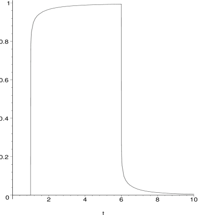
Figure 1: Typical shape of the signal (for illustration we take the initial profile to have unit amplitude and duration $T=5$, “size” of the extra dimensions is $L=0.1$): forefront screening and the tail after backfront.

Finally, there is one more interesting effect: deformation of the forefront of the signal. It is due to the second term in equation (4.15). Noting the negative sign of this term it effectively leads to a relative screening of the purely 4-dimensional part of the signal. The typical shape of the resultant signal is shown in Fig.1. In order to analyse this effect it is useful to rewrite eq.(4.15) once again

$$\Big{<}\Phi(t,{\mathbf{x}})\Big{>}\simeq\Phi_{0}(t,{\mathbf{x}})+\Phi_{1}(t,{\mathbf{x}}),$$ (4.19)

$$\Phi_{0}(t,{\mathbf{x}})=\frac{G_{4}}{4\pi r},$$ (4.20)

$$\Phi_{1}(t,{\mathbf{x}})=-\frac{G_{4}}{6\pi^{2}r}\,\frac{2^{5/2}-5}{\alpha(t)^{1/2}}=-\frac{2}{3\pi}\,\frac{2^{5/2}-5}{\alpha(t)^{1/2}}\;\Phi_{0}(t,{\mathbf{x}})~{}~{},\,\,\,$$ (4.21)

where we assumed that $r<t<r+T$ so that no contribution of the backfront is yet present, in terms of parameter $\alpha(t)=(t^{2}-r^{2})^{1/2}/2L$ having the meaning of number of spikes that have already passed through the observer by the time of observation. This number is supposed to be sufficiently large to guarantee the formation of the four-dimensional signal (the first term in eq.(4.15)). It also should be relatively small for the relation $t\sim r$ to hold. Eventually, the minimal value of $\alpha(t)$ is related to the time resolution of the measuring devise: it may not resolve a single spike, but should resolve the lapse between the arrival of the forefront and the observation moment $t$. Similar regime exists at the backfront tail: for $t$ close to $r+T$ the tail signal (4.17) is dominated by the number of spikes arriving right after the original signal ends. Later in the paper we will discuss possible observational implications in the gravitational astronomy of the tail effect (4.18) and, especially, the correction effect (4.21).

5. Periodic signal

In this section we consider the situation when the source on the brane radiates a periodic in time signal. So that we have

$$f(t)=e^{i\omega t}~{}~{},$$ (5.1)

where $\omega$ is the frequency of the signal, to be substituted in (4.4). The $t$-integral then is taken explicitly to produce

$$\int_{-\infty}^{t-r}{dt^{\prime}\,e^{i\omega t^{\prime}}\over\sqrt{(t-t^{\prime})^{2}-r^{2}}}={(-\pi i)\over 2}\,e^{i\omega t}\,H^{(2)}_{0}(\omega r)~{}~{},$$ (5.2)

so that the gravitational field takes the form

$$\Phi(r,t)=-{G_{5}\over 8\pi i}e^{i\omega t}\,{1\over r}\,\partial_{r}\sum_{n=-\infty}^{+\infty}H^{(2)}_{0}(\omega\sqrt{r^{2}+4n^{2}L^{2}})~{}~{}.$$ (5.3)

A possible way to estimate the infinite sum is to replace it by integral. This approximation is valid when $\omega\,L<<1$. Then we have that

$$\sum_{n=-\infty}^{+\infty}H^{(2)}_{0}(\omega\sqrt{r^{2}+4n^{2}L^{2}})\simeq 2\int_{0}^{\infty}dxH^{(2)}_{0}(\omega\sqrt{r^{2}+4L^{2}x^{2}})={1\over L\omega}\,e^{-i\omega r}~{}~{},$$ (5.4)

where in the passing to the last expression a table integral available in [8] has been used. Thus, to the leading order the gravitational signal is

$$\Phi(r,t)\simeq\Phi_{0}(r,t)={G_{4}\over 8\pi r}\,e^{i\omega(t-r)}~{}~{}.$$ (5.5)

It is exactly the shape of the purely 4-dimensional signal arising from a periodic source. Thus, by replacing the sum over images in (5.3) with the integral we have explicitly demonstrated our earlier statement that the 4-dimensional physics is recovered from 5-dimensional as a superposition of signals from infinite number of images. In order to get a correction to the four-dimensional result (5.5) we have to estimate a deviation of the integral in (5.4) from the sum. First, we estimate this deviation for a single term in the sum (by expanding the integrand to first term of its Taylor series),

$$H^{(2)}_{0}(\omega\sqrt{r^{2}+4n^{2}L^{2}})-\int_{n}^{n+1}dx\,H^{(2)}_{0}(\omega\sqrt{r^{2}+4n^{2}x^{2}})$$

$$=\int_{n}^{n+1}dx\,(H^{(2)}_{0}(\omega\sqrt{r^{2}+4n^{2}L^{2}})-H^{(2)}_{0}(\omega\sqrt{r^{2}+4L^{2}x^{2}}))$$

$$\simeq{2\,n\,L^{2}\omega\over\sqrt{r^{2}+4L^{2}n^{2}}}H_{1}^{(2)}(\omega\sqrt{r^{2}+4L^{2}n^{2}})~{}~{}.$$ (5.6)

Summing now this deviation for all $n$ and again replacing the sum by the integral (which turns out to be exactly integrable in view of the relation $H_{1}^{(2)}(z)=(d/dz)H_{0}^{(2)}(z)$) we find

$$\int_{0}^{\infty}dx{2xL^{2}\omega\over\sqrt{r^{2}+4L^{2}x^{2}}}H_{1}^{(2)}(\omega\sqrt{r^{2}+4L^{2}x^{2}})={1\over 2}H^{(2)}_{0}(\omega r)~{}~{}.$$ (5.7)

Thus we find that the correction $\Phi_{1}(r,t)$ to the purely 4-dimensional result (5.4) is

$$\Phi_{1}(r,t)={G_{4}\over 8\pi i}{L\omega\over r}\,e^{i\omega t}\,H^{(2)}_{1}(\omega r)~{}~{},$$ (5.8)

We are interested in a limit when the value of $\omega r$ is large. Then we can use the asymptotic formula for the Hankel function and get

$$\Phi_{1}(r,t)\simeq{G_{4}\over 8\pi}\,\sqrt{2\over\pi}\,{L\sqrt{\omega}\over r^{3/2}}\,e^{i\omega(t-r)+i{\pi\over 4}}=\sqrt{\frac{2L^{2}\omega}{\pi r}}\,e^{i\pi/4}\,\Phi_{0}(r,t)~{}~{}.$$ (5.9)

This part of the signal is entirely due to the extra dimension. Notice the phase shift with respect to the 4-dimensional signal (5.5). Also, the amplitude of (5.9) now depends on the frequency of the signal. These two circumstances help to distinguish the purely 4-dimensional part of the signal from that of due to presence of the extra dimension. We see that one of the manifestations of the fifth dimension is some frequency-dependent amplification of the amplitude $|\Phi_{0}(r,t)+\Phi_{1}(r,t)|$ of the signal from a periodic source.

6. Can gravitational antenna detect the extra
dimension?

Our analysis shows that there are two, at least in principle observable, effects of the compact fifth dimension on the propagation of the gravitational signal. First, it is the tail effect discussed in section 4: after a signal of finite duration $T$ has passed through the observer there still remains a tail signal (4.18) entirely due to the presence of extra dimension. The late-time tail signal is a power decaying function of time, $t^{-5/2}$. In the four-dimensional physics the tail does not appear at all. Therefore, its observation would be a clear evidence for the fifth dimension. The amplitude of the purely four-dimensional signal at distance $r$ from the source is the usual Newton potential (4.20), $\Phi_{0}(t,r)=G_{4}/4\pi r$. Measuring the amplitude of the tail (4.18) with respect to $\Phi_{0}$ we find that the upper bound on this ratio is given by the quantity

$$\chi\sim{L^{1/2}T\over r^{3/2}}\,~{}~{},$$ (6.1)

where we took the observation moment $t\geq r$.

Another effect comes for a periodic signal of frequency $\omega$ from a source placed at distance $r$ from the point of observation. The signal is amplified due to multiple winding around the compact extra dimension, moreover the correction component (5.9) has a phase shift useful for observational purposes. The amplification factor is $1+\eta$ where $\eta$ according to (5.9) behaves as

$$\eta\sim{L\over\sqrt{\lambda r}}~{}~{},$$ (6.2)

in terms of the wavelength $\lambda=2\pi/\omega$ of the signal (in our units the speed of light $c=1$).

The two effects suggest that the extra dimension in principle could be observed in gravitational wave experiments and thus may have some consequences for the gravitational astronomy. The effects governed by parameters $\chi$ or $\eta$ are however expected to be extremely small. Here we give some estimates adjusted for the parameters (see for example [12] and [13]) of the LIGO and LISA detectors. The sensitivity of the LISA detector covers a low frequency range $10^{-4}-1$ Hz. For a source placed at distance of 10 Mpc from the Earth and producing a signal of finite duration $T\sim 10^{4}$ s (associated with the inverse of the lower bound of this frequency band) we have, assuming that the size of the extra dimension $L\sim 10^{-1}$ cm, that $\chi\sim 10^{-25}$. The LIGO detector is sensitive for a higher frequency, $1-10^{4}$ Hz, and is more appropriate for the observation of the amplification effect for a periodic signal. For the frequency $\omega\sim 100$ Hz and the distance of 10 Mpc we find that $\eta\sim 10^{-18}$. The observation of the amplification effects thus requires less amplitude sensitivity of the gravitational antenna. We should not forget, however, that $\eta$ (or $\chi$) should be further multiplied by the amplitude of the purely four-dimensional signal to give the value for the amplitude of the interesting part of the signal. The resultant effect then is too small to be experimentally observable now or in coming future. It is nevertheless worth noting that the late time tail (4.18) does not depend on the distance from the source. Therefore, there might be a cumulative effect of superposition of the tails from large number of various sources. The resultant signal is proportional to the number of sources (both recent and in very distant past) in our part of the Universe and thus may have a much larger amplitude and can be singled out by the characteristic $t^{-5/2}$ behavior.

There is yet another range of observation intervals which gives more hope for experimental detection. This range corresponds to (4.19)-(4.21) – the transition regime from the moment of the arriving forefront of the signal at $t=r$ to late times $t>r$. In this regime the time is sufficiently larger than $r$ to generate a large number $\alpha(t)$ of signal spikes – signals from images that already reached the observer – but not big enough to relax to negligible small tail rapidly decaying with time. This number $\alpha(t)$ should be high enough to guarantee the formation of the four-dimensional signal (4.19) (remember that it gets completely recovered at infinite $t$ as a cumulative effect of an infinite number of images), but it should not be too big so that antenna would be able to resolve the lapse after arriving the forefront and the observation time. The correction to the 4-dimensional signal is given by the product $\alpha(t)^{-1/2}\Phi_{0}(t,{\mathbf{x}})$. The lower bound on $\alpha$ is related to the time resolution $\Delta t$ of the antenna as $[{\rm min}~{}\alpha]\sim({\Delta t\over L})^{1/2}~{}({r\over L})^{1/2}$. This gives an estimate $\alpha^{-1/2}\sim 10^{-8}$ (adjusted to the frequency $10^{4}$ Hz available at LIGO) and it makes certainly a much stronger effect than the ones that have been just discussed.

Thus, the idea of echoing extra dimension(s) by the gravitational-wave astronomy looks feasible, and we are planning to return to this issue in subsequent publications.

Appendix A. Alternative derivation of the retarded Green’s function

The retarded Green’s function of the massive Klein-Gordon operator in four dimensions has a representation in terms of the Bessel function of zeroth order [10, 11]

$$G_{R}(m^{2}|\,t,{\mathbf{x}})=-\frac{1}{4\pi r}\,\frac{\partial}{\partial r}\,\Big{[}\,J_{0}(m\sqrt{t^{2}-r^{2}})\theta(t-r)\,\Big{]}~{}~{}.$$ (A.1)

Therefore, the retarded version of the equation 2.8 involves summation over the tower of Kaluza-Klein masses $m_{n}=n\pi/L$. This summation can be done with the aid of the Eq.(8.522) of [8]

$$\sum\limits_{n=-\infty}^{\infty}J_{0}(n\pi s/L)=\frac{2L}{\pi}\sum\limits_{n=-m}^{m}\frac{1}{\sqrt{s^{2}-4n^{2}L^{2}}}~{}~{},$$ (A.2)

where $m$ is the integer satisfying the inequalities

$$2m<s/L<2(m+1)~{}~{}.$$ (A.3)

This can be rewritten for $s=\sqrt{t^{2}-r^{2}}$ as

$$\sum\limits_{n=-\infty}^{\infty}J_{0}(n\pi\sqrt{t^{2}-r^{2}}/L)=\frac{2L}{\pi}\sum\limits_{n=-\infty}^{\infty}\frac{\theta(t-\sqrt{r^{2}+4n^{2}L^{2}})}{\sqrt{t^{2}-r^{2}-4n^{2}L^{2}}}~{}~{},$$ (A.4)

so that the resultant expression for the retarded Green’s function is given by equation (3.11) in the main text.

Appendix B. Calculation of $I(\alpha,\beta\,|\,m)$

The calculation of the finite sum (4.9) is based on the following representation of this sum in terms of the contour integral in the complex plane of the summation parameter $z$

$$I(\alpha,\beta\,|\,m)=\frac{\pi}{\beta}\,\frac{\coth\pi\beta}{\sqrt{\alpha^{2}+\beta^{2}}}+\frac{1}{2i}\int\limits_{{\mathbf{C}}_{m}}dz\,\frac{\cot\pi z}{(\beta^{2}+z^{2})\sqrt{\alpha^{2}-z^{2}}}~{}~{}.$$ (B.1)

The closed contour of integration ${\mathbf{C}}_{m}$ here consists of the four lines,

$${\mathbf{C}}_{m}={\mathbf{C}}_{m}^{+}\cup{\mathbf{C}}_{m}^{-}\cup{\mathbf{C}}^{+\infty}\cup{\mathbf{C}}^{-\infty},$$

$${\mathbf{C}}_{m}^{\pm}:\,\,z=\pm m+iy,\,\,-\infty<y<\infty,$$

$${\mathbf{C}}^{\pm\infty}:\,\,z=x\pm i\infty,\,\,-m<x<m~{}~{},$$ (B.2)

forming a rectangle gone around in anti-clockwise way. The contour integral in (B.1) gives the sum of contributions of residues at the poles of $\cot\pi z$ which reproduce the needed finite sum (4.9) and the sum of two residues of the integrand at $z=\pm i\beta$ compensated by the first term on the right hand side of (B.1).

The integrals over ${\mathbf{C}}^{\pm\infty}$ obviously give zero contribution, while the integrals over ${\mathbf{C}}_{m}^{+}\cup{\mathbf{C}}_{m}^{-}$ in view of the relation

$$\cot\pi(\pm m+iy)=-i\coth\pi y=-i\left(1+\frac{2}{e^{2\pi y}-1}\right)$$ (B.3)

can be reduced to the sum of the following contributions of the integral over the segment of the real axis, $-m\leq z\leq m$, the residue of the integrand at $z=+i\beta$ and the thermal-type integral

$$\frac{1}{2i}\int\limits_{{\mathbf{C}}_{m}}dz\,\frac{\cot\pi z}{(\beta^{2}+z^{2})\sqrt{\alpha^{2}-z^{2}}}=-\frac{\pi}{\beta\sqrt{\alpha^{2}+\beta^{2}}}+\int_{-m}^{m}\frac{dx}{(\beta^{2}+x^{2})\sqrt{\alpha^{2}-x^{2}}}$$

$$\qquad\qquad\qquad\qquad\qquad\qquad\qquad-2i\int\limits_{0}^{\infty}dy\,\frac{1}{e^{2\pi y}-1}\,\Big{(}f(y)-f(-y)\Big{)}~{}~{},$$ (B.4)

where the function $f(y)$ equals

$$f(y)=\left.\frac{1}{(\beta^{2}+z^{2})\sqrt{\alpha^{2}-z^{2}}}\,\right|_{\,z=m+iy}~{}~{}.$$ (B.5)

Since

$$\int_{-m}^{m}\frac{dx}{(\beta^{2}+x^{2})\sqrt{\alpha^{2}-x^{2}}}=\frac{2}{\beta\sqrt{\alpha^{2}+\beta^{2}}}\arctan\left(\frac{\sqrt{\alpha^{2}+\beta^{2}}}{\beta}\,\frac{m}{\sqrt{\alpha^{2}-m^{2}}}\right)$$ (B.6)

we finally have

$$I(\alpha,\beta\,|\,m)=\frac{\pi}{\beta}\,\frac{\coth\pi\beta-1}{\sqrt{\alpha^{2}+\beta^{2}}}+\frac{2}{\beta\sqrt{\alpha^{2}+\beta^{2}}}\,\arctan\left(\frac{\sqrt{\alpha^{2}+\beta^{2}}}{\beta}\,\frac{m}{\sqrt{\alpha^{2}-m^{2}}}\right)$$

$$\qquad\qquad\qquad\qquad-2i\int\limits_{0}^{\infty}dy\,\frac{1}{e^{2\pi y}-1}\,\Big{(}f(y)-f(-y)\Big{)}~{}~{}.$$ (B.7)

So far it was exact calculation without any approximation made. We are now interested in the limit of large $\alpha$. The calculation of the last integral in (B.7) for $\alpha\gg 1$ follows from the asymptotic expression for the combination of functions $f(\pm y)$ in (B.7)

$$f(y)-f(-y)=\frac{i}{\sqrt{\alpha\delta}}\,\frac{1}{\alpha^{2}+\beta^{2}}\,\sqrt{\frac{(1+y^{2}/\delta^{2})^{1/2}-1}{1+y^{2}/\delta^{2}}}\,\left(\,1+{\rm O}\left(\frac{1}{\alpha^{1/2}}\right)\right)~{}~{},$$ (B.8)

where the parameter $\delta=\alpha-m$ is of order unity (bearing in mind that $m$ will be identified with $[\alpha]$). Thus the integral in (B.7) after rescaling the integration variable $y\to y\delta$ becomes

$$-2i\int\limits_{0}^{\infty}dy\,\frac{1}{e^{2\pi y}-1}\,\Big{(}f(y)-f(-y)\Big{)}=\frac{2}{\alpha^{2}+\beta^{2}}\sqrt{\frac{\delta}{\alpha}}\,I(\delta)\,\left(\,1+{\rm O}\left(\frac{1}{\alpha^{1/2}}\right)\right)~{}~{},$$ (B.9)

where $I(\delta)$ is defined by Eq.(4.11).

In the expression for the retarded potential (4.6) the parameter $m$ should be taken coinciding with $[\alpha]$. Then for integer values of $\alpha$ the parameter $\delta$ will be vanishing and $I(\delta)$ will be divergent. To isolate these divergences we disentangle from the sum (4.9), $I(\alpha,\beta\,|\,[\alpha])$, the potentially divergent terms at $n=\pm[\alpha]$,

$$I(\alpha,\beta\,|\,[\alpha])=I(\alpha,\beta\,|\,[\alpha]-1)+\frac{2}{(\beta^{2}+[\alpha]^{2})\sqrt{\alpha^{2}-[\alpha]^{2}}}~{}~{}.$$ (B.10)

The last term here becomes singular at integer values of $\alpha$, but the first term is absolutely finite, because its corresponding value of $\delta=\alpha-[\alpha]+1$ belongs to the range $1\leq\delta<2$. Therefore, using in (B.10) the equation (B.7) with $m=[\alpha]-1$ and expanding the arctangent

$$\frac{2}{\beta\sqrt{\alpha^{2}+\beta^{2}}}\,\arctan\left(\frac{\sqrt{\alpha^{2}+\beta^{2}}}{\beta}\,\frac{[\alpha]-1}{\sqrt{\alpha^{2}-([\alpha]-1)^{2}}}\right)$$

$$=\frac{\pi}{\beta\sqrt{\alpha^{2}+\beta^{2}}}-\frac{2^{3/2}}{\alpha^{2}+\beta^{2}}\,\sqrt{\frac{\alpha-[\alpha]+1}{\alpha}}+{\rm O}\left(\frac{1}{\alpha^{7/2}}\right)$$ (B.11)

one finally obtains the expression (4.10) used in Sect.4.

References

- [1] V. A. Rubakov, “Large and infinite extra dimensions: An introduction,” Phys. Usp. 44, 871 (2001) [Usp. Fiz. Nauk 171, 913 (2001)] [arXiv:hep-ph/0104152]
- [2] G. E. Shilov, Generalized functions and partial differential equations, (Gordon and Breach, New York, 1968).
- [3] D. V. Galtsov, “Radiation reaction in various dimensions,” Phys. Rev. D 66, 025016 (2002) [arXiv:hep-th/0112110].
- [4] V. Frolov, M. Snajdr and D. Stojkovic, “Interaction of a brane with a moving bulk black hole,” arXiv:gr-qc/0304083.
- [5] V. Cardoso, O. J. C. Dias and J. P. S. Lemos, “Gravitational Radiation in D-dimensional Spacetimes,” Phys. Rev. D 67 064026 (2003), [arXiv:hep-th/0212168].
- [6] A. O. Barvinsky and D. V. Nesterov, “Duality of boundary value problems and braneworld action in curved brane models,” Nucl. Phys. B 654, 225 (2003) [arXiv:hep-th/0210005].
- [7] M. K. Parikh and S. N. Solodukhin, “De Sitter brane gravity: From close-up to panorama,” Phys. Lett. B 503, 384 (2001) [arXiv:hep-th/0012231].
- [8] I. S. Gradstein and I. M. Ryzhik, Table of Integrals, Series, and Products, (Academic Press, New York and London, 1965).
- [9] B. S. De Witt, Dynamical Theory of Groups and Fields, (Gordon and Breach, New York, 1965).
- [10] F. W. Byron and R. W. Fuller, Mathematics of classical and quantum physics. Vol. 2. (Addison-Wesley, 1970).
- [11] R. Gregory, V. A. Rubakov, S. M. Sibiryakov, “Brane worlds: The gravity of escaping matter,” Class. Quant. Grav. 17 4437 (2000), [arXiv:hep-th/0003109].
-
[12]
B. Barish, LIGO Overview, NSF Annual Report, 23 Oct. 2002
http://www.ligo.caltech.edu/LIGO_web/conferences/nsf_reviews.html - [13] S. A. Hughes, “Listening to the universe with gravitational-wave astronomy,” Annals Phys. 303, 142 (2003) [arXiv:astro-ph/0210481].