DCPT-03/29

Thermodynamic Bethe ansatz for the AII $\sigma$-models

Andrei Babichenko and Roberto Tateo^,

¹Shahal str., 73/4, Jerusalem, 93721, Israel

²Dept. of Mathematical Sciences, University of Durham, Durham DH1 3LE, UK

³Dipartimento di Fisica Teorica, Università di Torino, Via P. Giuria 1, 10125 Torino, I

We derive thermodynamic Bethe ansatz equations describing the vacuum energy of the $SU(2N)/Sp(N)$ nonlinear sigma model on a cylinder geometry. The starting points are the recently-proposed amplitudes for the scattering among the physical, massive excitations of the theory. The analysis fully confirms the correctness of the S-matrix. We also derive closed sets of functional relations for the pseudoenergies (Y-systems). These relations are shown to be the $k\rightarrow\infty$ limit of the $Sp(k+1)$-related systems studied some years ago by Kuniba and Nakanishi in the framework of lattice models.

PACS: 02.30.Ik; 11.25.Hf; 11.10.-z
Keywords: Nonlinear sigma models; Integrable models; Finite-size scaling; Thermodynamic Bethe ansatz

1 Introduction

Since the early days of modern particle physics, the interest in four dimensional non-Abelian gauge theories has also strongly encouraged the study of two dimensional nonlinear sigma models. The main, well-known reason is that the two theories share the remarkable properties of renormalizability, confinement and asymptotic freedom. Besides the obvious advantage of working in a lower dimensional setup, many 2D nonlinear sigma models exhibit the even more useful property of integrability. Exact solubility offers the unique opportunity to investigate non perturbative phenomena in quantum field theory and statistical mechanics via non perturbative tools like the exact S-matrix [1], the Form Factor [2] and the thermodynamic Bethe ansatz [3] (TBA) methods. Along the lines of the earlier work by Fateev and Zamolodchikov [4] but also motivated by new, interesting applications in condensed matter physics and string theory [5] there has been recently a renewed interest in 2D integrable sigma models [6, 7, 8, 9, 10, 11, 12, 13] .

When dealing with an integrable quantum field theory, a well established strategy is to derive the scattering matrix by solving suitably imposed Yang-Baxter equations, together with the unitary and crossing constraints. The S-matrix, via the so-called bootstrap procedure, gives access to the full infrared mass spectrum of the theory and via the Form Factors, to the large distance behaviour of correlation functions.

In order to explore the ultraviolet phase of the model and, at the same time, to check the correctness of the S-matrix, the standard tool is the thermodynamic Bethe ansatz. The TBA method is susceptible to all the details of the scattering matrix, it uses the full mass spectrum and it is sensitive to the ambiguous (CDD) scalar factors contributing to the amplitudes. It leads to numerically solvable integral equations for the vacuum energy on a cylinder geometry and exact values for central charge and scaling dimensions of the conformal field theory (CFT) describing the model in its deep ultraviolet limit.

Following the idea of Zamolodchikov [14], and starting from a given TBA equation, it is possible to derive sets of functional relations called Y-systems. The Y-systems are “universal” in the sense that there is a one–to–many correspondence with TBAs. A Y-system can be transformed by imposing different analytic properties, to physically distinct TBAs. (The relationship between Y-systems and TBA equations is practically the same as the one between differential equations and their solutions.)

Many examples of functional relations which exhibit elegant Lie algebraic-related structures are now known. Most of them are, or were at some stage, purely conjectures (see, for example, [15, 16, 17, 18, 19, 20, 21, 22, 23, 24, 25]). An important family of such systems is encoded on a pair of Dynkin diagrams of ADE type [20, 21, 22]; a second family is in correspondence with all the simple Lie algebras and it was studied in the works by Kuniba and Nakanishi [17] in the closely related framework of integrable lattice models. Many, but by no means all, solutions of these systems have been successfully related to perturbations of minimal CFTs and to sigma models [3, 4, 6, 8, 16, 17, 18, 19, 20, 21, 22, 23, 24, 25, 26, 27].

In this paper, such an example of TBA system is derived in the context of integrable nonlinear sigma models. Being infinite in one direction, the equations require a truncation for the ultraviolet analysis. The truncated systems are found to describe the perturbation of the coset $SU(2N)_{k+1}/Sp(N)_{k+1}$ via the relevant operator $(1,adj)$.

The starting point is the recently proposed [12] S-matrix for the sigma models defined on the symmetric space AII. (This space is isomorphic to the group coset manifold $SU(2N)/Sp(N)$.) The S-matrix is of $SU(2N)$ Gross-Neveu type, with CDD factors modified in such a way that their poles describe only the particle multiplets related to the even fundamental weights of $SU(2N)$.

The plan of the paper is as follows. The model is briefly introduced in section 2. The derivation of the TBA equations is sketched in section 3. The Y-system is derived in section 4 and its equivalence to a particular limit of the $C_{k+1}$-related system of [17] is discussed in section 5. Using the dilogarithm identities of [17] the ultraviolet central charge is found to be $c=2N^{2}-N-1$: a result which is fully consistent with the interpretation of the model as a perturbation of the $SU(2N)/Sp(N)$ conformal field theory. Section 6 contains our conclusions, while the explicit definitions of the kernel functions are collected in the appendix at the end of the paper.

2 The AII sigma models

The classical action of the quantum field theory in question is defined through the functional

$$S[g]={1\over\lambda^{2}}\int d^{2}xTr[\partial_{\mu}g(x)\partial_{\mu}g^{-1}(x)]~{},$$ (1)

where $g(x)$ belongs to a matrix representation of $SU(2N)$ constrained on the symmetric space $SU(2N)/Sp(N)$. Then the action $S_{NLSM}[\phi]\equiv S[g(\phi)]$ of the model is obtained from $S[g]$ by solving the constraint in terms of the independent set of fields $\{\phi\}$ and substituting the resulting $g(\phi(x))$ into (1).

The spectrum of the AII sigma models consists in multiplets transforming in the representations with even fundamental highest weights $\mu_{2a}$ of $SU(2N)$. The masses of these multiplets are

$$m_{2a}=M\sin\left(\frac{\pi a}{N}\right),~{}~{}~{}~{}a=1,...,N-1~{},$$ (2)

($M=M(\lambda)$ is the mass scale). The amplitude $S_{2a,2b}$ for scattering of a particle $2a$ on the particle $2b$ is obtained by fusion of $S_{2,2}$. The latter was proposed in [12], and has the form [28]

$$S_{2a,2b}(\theta)=X_{2a,2b}(\theta)\sigma_{2a,2b}(\theta)\widetilde{S}_{2a,2b}(\theta)~{}~{}.$$ (3)

$\widetilde{S}_{2a,2b}(\theta)$ is the $SU(2N)$ invariant R-matrix spectral decomposed into its irreducible representations [29], $\sigma_{2a,2b}(\theta)$ is the cross-unitarity factor and $X_{2a,2b}(\theta)$ is again obtained by fusion of $X_{2,2}(\theta)$. They have the following forms [29, 28]

$$X_{2a,2b}(\theta) = \prod_{i=1}^{a}\prod_{j=1}^{b}X(\theta+4\pi i\Delta(i+j-1-\frac{a+b}{2}))$$ (4)

$$= \exp\left\{-\int_{-\infty}^{\infty}\frac{d\omega}{\omega}e^{i\frac{g}{\pi}\theta\omega}\left(\widehat{A}_{2a,2b}^{(2N)}(\omega)-\delta_{ab}\right)\right\}~{},$$

with $g=2N$, $\Delta=\frac{1}{g}$, and

$$X(\theta)=\frac{\sinh((\theta+4\pi i\Delta)/2)}{\sinh((\theta-4\pi i\Delta)/2)}~{},~{}~{}~{}~{}~{}\sigma_{2a,2b}(\theta)=\exp\left\{\int_{-\infty}^{\infty}\frac{d\omega}{\omega}e^{i\frac{g}{\pi}\theta\omega}\widehat{\Psi}_{2a,2b}(\omega)\right\}~{}.$$ (5)

The explicit expressions of $\widehat{A}_{2a,2b}^{(2N)}(\omega)$ and $\widehat{\Psi}_{2a,2b}(\omega)$ are given in the appendix at the end of the paper. (Notice that the factor $X_{2a,2b}(\theta)$ is the same as $X_{ab}(\theta)$ in the $SU(2N)$ invariant Gross-Neveu model of [29], however the $\widehat{A}_{2a,2b}^{(2N)}(\omega)$ are different. This is because an N-dependent form of the Fourier transform is used in this paper.) Using these expressions we find

$$\sigma_{2a,2b}(\theta)X_{2a,2b}(\theta)=\exp\left\{-\int_{-\infty}^{\infty}\frac{d\omega}{\omega}e^{i\frac{g}{\pi}\theta\omega}\left(\widehat{Y}_{2a,2b}(\omega)-\delta_{ab}\right)\right\}~{},$$ (6)

$$\widehat{Y}_{2a,2b}(\omega)=\frac{e^{|\omega|}}{\cosh\omega}\frac{\sinh(2|\omega|\min(a,b))\sinh(2\omega(N-\max(a,b)))}{\sinh(2\omega N)}~{}.$$ (7)

3 Diagonalisation of the transfer matrix and the TBA equations

The standard derivation of the TBA equations starts by imposing periodicity conditions on the wavefunction describing a gas of particles with rapidity set $\{\theta_{l}\}$ and confined on a ring of circumference $\cal{L}$. The quantisation condition is

$$e^{im_{2a_{j}}{\cal L}\sinh\theta_{j}}~{}T^{2a_{j}}(\theta_{j}|\theta_{j+1},...,\theta_{\cal{N}},\theta_{1},...,\theta_{j-1})=1~{},$$ (8)

$T^{2a_{j}}$ is the transfer matrix and it is constructed out of the S-matrix as

$$T^{2a_{j}}(\theta_{j}|\theta_{j+1},...,\theta_{\cal{N}},\theta_{1},...,\theta_{j-1})=-\mbox{Tr}\left[S_{2a_{j},2a_{1}}(\theta_{j}-\theta_{1})\dots S_{2a_{j},2a_{\cal N}}(\theta_{j}-\theta_{\cal N})\right]~{},$$ (9)

where the trace is over the representation of the particle of type $2a_{j}$. The main problem is then to find the largest eigenvalue $T_{0}$ of $T$. The solution is [30]

$$T_{0}^{2a_{j}}=\prod_{i=1,i\neq j}^{\cal{N}}X_{2a_{j},2a_{i}}(\theta_{j}-\theta_{i})~{}\sigma_{2a_{j},2a_{i}}(\theta_{j}-\theta_{i})\times\prod_{\alpha=1}^{M_{2a_{j}}}\left(\frac{\theta_{j}-v_{\alpha}^{(2a_{j})}+i\pi\Delta}{\theta_{j}-v_{\alpha}^{(2a_{j})}-i\pi\Delta}\right)~{}.$$ (10)

In equations (10), the set of parameters $\{v_{\alpha}^{(b)}\}$ is solution of the Bethe equation [29, 30]

$$\prod_{j=1}^{\cal{N}}\left(\frac{v_{\alpha}^{(b)}-\theta_{j}+i\pi\Delta\omega_{a_{j}}\cdot\alpha_{b}}{v_{\alpha}^{(b)}-\theta_{j}+i\pi\Delta\omega_{a_{j}}\cdot\alpha_{b}}\right)=\Omega_{\alpha}^{(b)}\prod_{c=1}^{2N-1}\prod_{\beta=1}^{M_{c}}\left(\frac{v_{\alpha}^{(b)}-v_{\beta}^{(c)}+i\pi\Delta\alpha_{b}\cdot\alpha_{c}}{v_{\alpha}^{(b)}-v_{\beta}^{(c)}-i\pi\Delta\alpha_{b}\cdot\alpha_{c}}\right)~{}.$$ (11)

$\omega_{b}$ and $\alpha_{b}$ are, respectively, the fundamental weights and roots of $SU(2N)$, $M_{c}$ is the number of solutions of type $c$, and $\Omega_{\alpha}^{(b)}$ is a phase factor which is irrelevant for the current calculations. In the thermodynamic limit

$$\cal{N}\rightarrow\infty~{},~{}~{}~{}\cal{L}\rightarrow\infty~{},~{}~{}~{}\cal{N}/\cal{L}=\hbox{finite}~{},$$ (12)

the solutions of (11) group into complex “strings” of length $p$ and real part $v_{\alpha p}^{(b)}$

$$v_{\alpha}^{(b)}=v_{\alpha p}^{(b)}+i\pi\Delta(p+1-2k),~{}~{}k=1,2,...,p~{}.$$ (13)

Using (11) in equation (8) with $T$ replaced by $T_{0}$, introducing “magnon” densities $\rho_{p}^{b}(v)$ for the real parts of $v_{\alpha}^{(b)}$, densities $\sigma_{2a}(\theta)$ for the particles, and after writing the log of equations (8) and (11) in terms of the densities we obtain

$$\sigma_{2a}(\theta)+\widetilde{\sigma}_{2a}(\theta)=\frac{m_{2a}}{2\pi}\cosh\theta+\sum_{b=1}^{N-1}Y_{2a,2b}\ast\sigma_{2b}(\theta)-\sum_{p=1}^{\infty}a_{p}\ast\rho_{p}^{2a}(\theta)~{},~{}~{}(a=1,\dots,N-1)$$ (14)

$$a_{p}\ast\sigma_{c}(\theta)=\widetilde{\rho}_{p}^{c}+\sum_{q=1}^{\infty}\sum_{b=1}^{2N-1}A_{pq}^{(\infty)}\ast K_{cb}^{(2N)}\ast\rho_{q}^{b}(\theta)~{},~{}~{}~{}(c=1,\dots,2N-1)~{}.$$ (15)

(The symbol $\ast$ denotes the standard convolution.) In (15 ) $\widetilde{\sigma}_{2a}$ and $\widetilde{\rho}_{p}^{a}$ complement the densities of particles to the total densities of states, and are called densities of holes. The expressions for the kernels $A_{pq}^{(\infty)}$, $K_{ab}^{(N)}$ and $a_{p}$, together with some useful identities, are written in the appendix.

Solving the latter equation with respect to $\rho_{q}^{b}$ and plugging the solution into equation (14):

$$\widetilde{s}_{0}^{2a}(\theta) = \frac{m_{2a}}{2\pi}\cosh\theta-\sum_{b=1}^{N-1}\sum_{q=0}^{\infty}Z_{0q}^{(\infty)}\ast A_{2a,2b}^{(2N)}\ast s_{q}^{2b}(\theta)~{},~{}~{}~{}(a=1,\dots,N-1)$$ (16)

$$\widetilde{s}_{p}^{c}(\theta) = -\sum_{b=1}^{2N-1}\sum_{q=0}^{\infty}K_{pq}^{(\infty)}\ast A_{cb}^{(2N)}\ast s_{q}^{b}(\theta)~{},~{}~{}(c=1,\dots,2N-1)$$ (17)

where $p=1,2,\dots$,

$$s_{0}^{c}=\sigma_{0}^{c}~{},~{}~{}~{}~{}~{}\widetilde{s}_{0}^{c}=\widetilde{\sigma}_{0}^{c}~{},~{}~{}~{}~{}~{}s_{p}^{c}=\widetilde{\rho}_{p}^{c}~{},~{}~{}~{}~{}~{}\widetilde{s}_{p}^{c}=\rho_{p}^{c}~{},$$ (18)

and

$$\sigma_{0}^{2i+1}=\widetilde{\sigma}_{0}^{2i+1}=0~{}.$$ (19)

The new kernel $Z_{0q}^{(\infty)}$ has the following Fourier representation

$$\widehat{Z}_{0q}^{(\infty)}(\omega)=\widehat{K}_{0q}^{(\infty)}(\omega)\left(1-\frac{\delta_{q0}}{2\cosh^{2}(\omega)}\right)~{}.$$ (20)

From equation (17) we see that the excitations $\widetilde{s}_{p}^{2a}$ with $p=0$ are massive, whereas those with $p\geq 1$ are of magnonic type. The next step in the derivation is also standard: one looks for the minimum of the free energy $F=E-TS$ subject to the constraint (17).( $T$ is the temperature, $E$ and $S$ are, respectively, the energy and the entropy and are expressible in terms of the densities $s,\widetilde{s}$.) The final equations are

$$L_{0+}^{2a}(\theta)=Rm_{2a}\cosh\theta+\sum_{b=1}^{N-1}\sum_{q=0}^{\infty}A_{2a,2b}^{(2N)}\ast Z_{0q}^{(\infty)}\ast L_{q-}^{2b}(\theta)~{},~{}~{}~{}(a=1,\dots,N-1)$$ (21)

$$L_{p+}^{c}(\theta)=\sum_{b=1}^{N-1}\sum_{q=0}^{\infty}A_{cb}^{(2N)}\ast K_{pq}^{(\infty)}\ast L_{q-}^{b}(\theta)~{},~{}~{}(c=1,\dots,2N-1)$$ (22)

where $L_{p\pm}^{a}=\ln\left(1+e^{\pm\varepsilon_{p}^{a}}\right)$, $R=1/T$ and $\varepsilon_{p}^{a}=\widetilde{s}_{p}^{a}/s_{p}^{a}$ are the dressed energies (pseudoenergies). The free energy per unit length $f(R,M)$ is

$$f(R,M)=-\frac{1}{2\pi}\sum_{a=1}^{N-1}\int_{-\infty}^{\infty}d\theta\ m_{2a}\cosh\theta L_{0-}^{2a}(\theta)~{}.$$ (23)

In the ultraviolet limit, $RM\rightarrow 0$, $f(R,M)$ can be related to the central charge of the corresponding conformal field theory by

$$f(R,M)\sim-\frac{\pi}{6R^{2}}c_{UV}~{}.$$ (24)

For the AII sigma model, the natural expectation is

$$c_{UV}=\hbox{Dim}[SU(2N)]-\hbox{Dim}[Sp(N)]=2N^{2}-N-1~{}.$$ (25)

4 The Y-system

A Y-system is a set of functional relations among the unknown functions

$$Y_{p}^{a}(\theta)=e^{\varepsilon_{p}^{a}(\theta)}~{}.$$ (26)

To derive a Y-system from the TBA obtained in the previous section one starts from eq. (21) in Fourier representation, multiply it by $\widehat{K}^{(N)}(2\omega)$ and use properties (48) and (49) to get

$$\frac{\cosh(2\omega)}{\cosh(\omega)}\sum_{b=1}^{N-1}\widehat{K}_{ab}^{(N)}(2\omega)\widehat{L}_{0+}^{2b}(\omega)=\sum_{c=1}^{2N-1}\sum_{q=0}^{\infty}\widehat{K^{\prime}}_{0q}^{(\infty)}(\omega)\left(2\cosh(\omega)\delta_{c,2a}+I_{ac}^{(2N-1)}\right)\widehat{L}_{q-}^{b}(\omega)~{},$$ (27)

with

$$\widehat{K^{\prime}}_{0q}^{(\infty)}(\omega)=\left(1-\frac{\delta_{q0}}{2\cosh^{2}(\omega)}\right)\left(\delta_{q0}-\frac{\delta_{q1}}{2\cosh(\omega)}\right)~{}.$$ (28)

Equation (27) can also be written as

$$\displaystyle{\frac{\cosh(2\omega)}{\cosh(\omega)}\widehat{L}_{0+}^{2a}(\omega)-\frac{1}{2\cosh(\omega)}\sum_{b=1}^{N-1}I_{ab}^{(N-1)}\widehat{L}_{0+}^{2b}(\omega)=~{}~{}~{}~{}~{}~{}~{}~{}~{}~{}~{}~{}~{}~{}~{}~{}~{}~{}~{}~{}~{}~{}~{}~{}~{}~{}~{}~{}~{}~{}~{}~{}~{}~{}~{}~{}~{}}$$

$$\displaystyle{\frac{\cosh(2\omega)}{\cosh(\omega)}\widehat{L}_{0-}^{2a}(\omega)-\frac{1}{2\cosh(\omega)}\sum_{b=1}^{2N-1}I_{ab}^{(2N-1)}\widehat{L}_{1-}^{b}(\omega)-\widehat{L}_{1-}^{2a}(\omega)}~{}.$$ (29)

By using $L_{p+}^{a}-L_{p-}^{a}=\varepsilon_{p}^{a}$:

$$2\cosh(2\omega)\widehat{\varepsilon}_{0}^{2a}(\omega)+2\cosh(\omega)\widehat{L}_{1-}^{2a}(\omega)=\sum_{b=1}^{N-1}I_{ab}^{(N)}\widehat{L}_{0+}^{2b}(\omega)-\sum_{b=1}^{2N-1}I_{ab}^{(2N)}\widehat{L}_{1-}^{b}(\omega)~{},$$ (30)

or, equivalently

$$Y_{0}^{2a}(\theta+2i\pi\Delta)Y_{0}^{2a}(\theta-2i\pi\Delta) = \left(1+\frac{1}{Y_{1}^{2a}(\theta+i\pi\Delta)}\right)^{-1}\left(1+\frac{1}{Y_{1}^{2a}(\theta-i\pi\Delta)}\right)^{-1}$$ (31)

$$\times \prod_{b=1}^{N-1}\left(1+Y_{0}^{2b}(\theta)\right)^{I_{ab}^{(N-1)}}\prod_{b=1}^{2N-1}\left(1+\frac{1}{Y_{1}^{2b}(\theta)}\right)^{-I_{ab}^{(2N-1)}}~{}.$$

($a=1,\dots,N-1$.) The same procedure applied to equation (22) leads to a second set of functional relations of $SU(2N)$ Gross–Neveu type [16, 8]:

$$Y_{p}^{c}(\theta+i\pi\Delta)Y_{p}^{c}(\theta-i\pi\Delta)=\prod_{b=1}^{2N-1}\left(1+Y_{p}^{b}(\theta)\right)^{I_{cb}^{(2N-1)}}\prod_{q=0}^{\infty}\left(1+\frac{1}{Y_{q}^{c}(\theta)}\right)^{-I_{pq}^{(\infty)}}~{},$$ (32)

where $p=1,2,\dots,\infty$, $c=1,2,\dots,2N-1$ and by definition $Y_{0}^{2i+1}=\infty$. The Y-system (31,32) is pictorially represented in figure 1. There is a one-to-one correspondence between the Y functions and the nodes in the diagram. Black nodes correspond to massive pseudoenergies, while white ones are of magnonic type; a link connecting a node $(p,a)$ and a node $(p^{\prime},a^{\prime})$ indicates that when $Y^{a}_{p}$ appears on the l.h.s. of equation (32) (or (31)), there is a term containing $Y^{a^{\prime}}_{p^{\prime}}$ on the r.h.s. The kind of term on the r.h.s. is different for different styles, horizontal and vertical links. Arrows indicate one-way directed links.

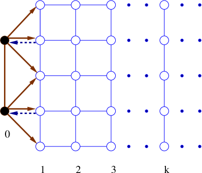
Figure 1: The TBA diagram for the $SU(6)/Sp(3)$ sigma model.

The ultraviolet central charge can then be written in terms of the sets of numbers $\{{\cal Y}_{p}^{a}\}$ and $\{{{\cal Y}^{\prime}}_{p}^{a}\}$, $\theta$-independent solutions of the full Y-system and of the subsystem obtained after eliminating all the massive nodes:

$$c_{UV}=\frac{6}{\pi^{2}}\left[\sum_{all\hskip 5.69046ptnodes}L\left(\frac{1}{1+{\cal Y}_{p}^{a}}\right)-\sum_{magnonic\hskip 5.69046ptnodes}L\left(\frac{1}{1+{{\cal Y}^{\prime}}_{p}^{a}}\right)\right]~{},$$ (33)

where $L$ is the Rogers dilogarithm function.

5 Truncation of the Y-system and its ultraviolet analysis

One of the main results of [17] is an exact conjecture for sum-rules of the type (33) for Y-systems related to the classical Lie algebras

$$\frac{6}{\pi^{2}}\sum_{all\hskip 5.69046ptnodes}L\left(\frac{{\cal Y}_{p}^{{a}{\bf[KN]}}}{1+{\cal Y}_{p}^{{a}{\bf[KN]}}}\right)=\frac{l~{}\hbox{Dim}[G]}{l+g^{\vee}}-\hbox{rank}[G]~{}.$$ (34)

Notice that the first term in the r.h.s. is the central charge of a WZW model for the algebra $G$ at level $l$ ($g^{\vee}$ is the dual Coxeter number). It is now easy to check that the Y-system (31,32) becomes equivalent to the $C_{k+1}$-related system of [17] at $l=N$, provided the infinite TBA diagram is truncated in the horizontal direction up to the node $k$ (see figure 1) and the following identifications are made

$$Y_{p}^{a}(\theta)=1/Y_{p}^{{a}{\bf[KN]}}(\theta)~{},~{}~{}~{}g^{\vee}=k+2~{},~{}~{}~{}\hbox{rank}[G]=k+1~{},$$ (35)

and hence

$$c_{1}=\frac{6}{\pi^{2}}\sum_{all~{}nodes}L\left(\frac{1}{1+{\cal Y}_{p}^{a}}\right)=\frac{N(k+1)(2(k+1)+1)}{N+k+2}-k-1~{}.$$ (36)

After the elimination of the massive nodes instead the correspondence is with a system of $A_{k}$ type at level $l=2N$. The second contribution to (33) is

$$c_{2}=\frac{6}{\pi^{2}}\sum_{magnonic~{}nodes}L\left(\frac{1}{1+{{\cal Y}^{\prime}}_{p}^{a}}\right)=\frac{2Nk(k+2)}{2N+k+1}-k~{}.$$ (37)

Notice now that

$$c_{1}-c_{2}=c[SU(2N)_{k+1}]-c[Sp(N)_{k+1}]~{},$$ (38)

is equal to the difference in the central charges of the $SU(2N)_{k+1}$ and $Sp(N)_{k+1}$ WZW models. It is then natural to conjecture that the level $k$ truncated system describes an integrable perturbation of the conformal model $SU(2N)_{k+1}/Sp(N)_{k+1}$. The perturbing operator is easily identified by noticing that the solutions of the Y-systems fulfil the periodicity property [14, 24]

$$Y_{p}^{a}\left(\theta+i\pi{N+k+2\over 2N}\right)=Y_{p}^{2N-a}(\theta)~{},$$ (39)

then the argument of [14] leads to the conformal dimensions

$$h=\bar{h}=1-{2N\over N+k+2}~{},$$ (40)

suggesting that the models in question are most certainly perturbed by the operator $(1,adj)$.

On the other hand, in the $k\rightarrow\infty$ limit $h=\bar{h}\rightarrow 1$ and

$$c_{UV}=\lim_{k\rightarrow\infty}(c_{1}-c_{2})=2N^{2}-N-1~{},$$ (41)

which is the expected result  (25) for the AII nonlinear sigma model.

6 Conclusions

The main purpose of this paper is to show that the $SU(2N)$ Gross–Neveu S-matrix, with a CDD factor selecting only even fundamental highest weight multiplets, correctly describes the ultraviolet limit of the sigma models on the AII symmetric spaces. Considering also the earlier result of [12], where the $(\mu_{2},\mu_{2})$ scattering amplitude was checked by comparing the free energy in strong external field with perturbation theory, we can confidently confirm the correctness of the proposal [12].

Another result of the paper is the mapping, through the Y-system, between our models and particular limits of systems proposed by Kuniba and Nakanishi in [17]. This led us to the interesting conjecture that the truncated TBA equations describe the coset $SU(2N)_{k+1}/Sp(N)_{k+1}$ models perturbed by the operator $(1,adj)$. As a follow-up project it would be interesting to check the integrability of these perturbed conformal field theories, to propose the exact S-matrix and to rigorously derive the set of thermodynamic equations.

A more general conclusion is again related to the interesting fact that the finite-size physics of these more exotic models is again described by set of equations of the kinds [17, 21]. It would be nice to understand this correspondence at a deeper level and to find the complete classification of the thermodynamic equations for integrable sigma models on symmetric spaces.

Acknowledgements

We are grateful to Patrick Dorey and Sergei Lukyanov for useful discussions. AB thanks the Mathematics Department of Durham University for hospitality while some of this work was in progress and RT thanks the EPSRC for an Advanced Fellowship.

7 Appendix

The definition of Fourier transform is

$$f(\theta)=g\int_{-\infty}^{\infty}\frac{d\omega}{2\pi^{2}}e^{i\frac{g}{\pi}\theta\omega}\widehat{f}(\omega)~{},~{}~{}~{}~{}\ \widehat{f}(\omega)=\int_{-\infty}^{\infty}d\theta~{}e^{-i\frac{g}{\pi}\theta\omega}f(\theta)~{},$$ (42)

where $g=2N$ is the dual Coxeter number of $SU(2N)$. The kernels $\widehat{A}_{ab}^{(L)}(\omega)$ and $\widehat{\Psi}_{2a2b}$ are

$$\widehat{A}_{ab}^{(L)}(\omega)=2\cosh(\omega)\frac{\sinh(\omega\min(a,b))\sinh(\omega(L-\max(a,b)))}{\sinh(\omega L)\sinh(\omega)}~{},$$ (43)

$$\widehat{\Psi}_{2a2b}(\omega)=e^{-|\omega|}\frac{\sinh(2\omega\min(a,b))\sinh(2\omega(N-\max(a,b)))}{\sinh(2\omega N)\sinh(\omega)}~{},$$ (44)

$$\widehat{K}_{ab}^{(L)}(\omega)=\left(\widehat{A}_{ab}^{(L)}(\omega)\right)^{-1}=\delta_{ab}-\frac{I_{ab}^{(L-1)}}{2\cosh(\omega)}~{},$$ (45)

$$\widehat{a}_{p}(\omega)=e^{-p|\omega|}~{}.$$ (46)

$I^{(L-1)}=2\delta_{ab}-C_{ab}^{A_{L-1}}$ and $C^{A_{L-1}}$ are, respectively, the incidence and Cartan matrices of the algebra $A_{L-1}$. The following relations are also useful

$$\sum_{b=1}^{\infty}\widehat{K}_{ab}^{(\infty)}(\omega)\widehat{a}_{b}(\omega)=\frac{\delta_{a1}}{2\cosh(\omega)}~{},$$ (47)

$$\sum_{b=1}^{N-1}\widehat{K}_{ab}^{(N)}(2\omega)m_{2b}\widehat{\cosh\theta}=0~{},$$ (48)

$$\sum_{b=1}^{N-1}\widehat{K}_{ab}^{(N)}(2\omega)\widehat{A}_{2b,c}^{(2N)}(\omega)=\frac{\cosh(\omega)}{\cosh(2\omega)}\left(2\cosh(\omega)\delta_{c,2a}+I_{2a,c}^{(2N)}\right)~{}.$$ (49)

In equation (48) $m_{2b}=M\sin\left(\frac{\pi b}{N}\right)$ is the Perron-Frobenius eigenvector of the $A_{N-1}$ Cartan matrix.

References

- [1] Al. B. Zamolodchikov and A. B. Zamolodchikov, ‘Factorized S-Matrices in two dimensions as the exact solutions of certain relativistic quantum field models’, Annals Phys. 120, (1979) 253.
- [2] F. A. Smirnov, ‘Form Factors in completely integrable models of quantum field theory’, World Scientific 1992.
- [3] Al. B. Zamolodchikov, ‘Thermodynamic Bethe ansatz in relativistic models. Scaling 3-state Potts and Lee-Yang models’, Nucl. Phys. B342, (1990) 695.
- [4] V. A. Fateev and Al. B. Zamolodchikov , ‘Integrable perturbations of parafermion models and the sigma model’, Phys. Lett. B271, (1991) 91.
- [5] J. Maldacena and L. Maoz, ‘Strings on pp-waves and massive two dimensional field theories’, JHEP 0212, (2002) 046, hep-th/0207284.
- [6] P. Fendley, ‘Sigma models as perturbed conformal field theories’, Phys. Rev. Lett. 83, (1999) 4468, hep-th/9906036.
- [7] P. Fendley, ‘Integrable sigma models with theta=’, Phys. Rev. B63, (2001) 104429, cond-mat/0008372.
- [8] P. Fendley, ‘Integrable sigma models and perturbed coset models’, JHEP 0105, (2001) 050, hep-th/0101034.
- [9] H. Saleur and B. Wehefritz-Kaufmann, ‘Integrable quantum field theories with OSP(m/2n) symmetries’, Nucl. Phys. B628, (2002) 407, hep-th/0112095.
- [10] J. Balog and A. Hegedus, ‘Virial expansion and TBA in O(N) sigma models’, Phys. Lett. B523, (2001) 211, hep-th/0108071.
- [11] J. Balog and P. Weisz, ‘Test of asymptotic freedom and scaling hypothesis in the 2d O(3) sigma model’, hep-th/0304214.
- [12] A. Babichenko, ‘Quantum integrability of sigma models on AII and CII symmetric spaces’, Phys. Lett. B554, (2003) 96, hep-th/0211114.
- [13] N. J. MacKay, ‘Rational K-matrices and representations of twisted Yangians’, J. Phys. A35, (2002)7865, math.qa/0205155.
- [14] Al. B. Zamolodchikov, ‘On the thermodynamic Bethe ansatz equations for the reflectionless ADE scattering theories’, Phys. Lett. B253, (1991) 391.
- [15] Al. B. Zamolodchikov, ‘Thermodynamic Bethe Ansatz for RSOS scattering theories’, Nucl. Phys. B358, (1991) 497.
- [16] Al. B. Zamolodchikov, ‘TBA equations for integrable perturbed coset models’, Nucl. Phys. B366, (1991) 122.
- [17] A. Kuniba and T. Nakanishi, ‘Spectra in conformal field theories from the Rogers dilogarithm’, Mod. Phys. Lett. A7, (1992) 3487, hep-th/9206034.
- [18] T. R. Klassen and E. Melzer, ‘Purely elastic scattering theories and their ultraviolet limits’, Nucl. Phys. B338, (1990) 485.
- [19] M. J. Martins, ‘The thermodynamic Bethe ansatz for deformed conformal field theories’, Phys. Lett. B277, (1992) 301, hep-th/9201032.
- [20] F. Ravanini, ‘Thermodynamic Bethe ansatz for coset models perturbed by their operator’, Phys. Lett. B282, (1992) 73, hep-th/9202020.
- [21] F. Ravanini, R. Tateo and A. Valleriani, ‘Dynkin TBA’s’, Int. J. Mod. Phys. A8, (1993) 1707, hep-th/9207040.
- [22] E. Quattrini, F. Ravanini and R. Tateo, ‘Integrable QFT(2) encoded on products of Dynkin diagrams’, published in “Quantum Field Theory and String Theory”, Nato ASI Series B: Physics Vol.328, (1995) 273, hep-th/9311116.
- [23] T. J. Hollowood, ‘From trigonometric S-matrices to the thermodynamic Bethe ansatz’, Phys. Lett. B320 (1994) 43, hep-th/9308147.
- [24] R. Tateo, ‘The Sine-Gordon Model as perturbed coset theory and generalizations’, Int. J. Mod. Phys. A10, (1995) 1357, hep-th/9405197.
- [25] P. Dorey, A. Pocklington and R. Tateo, ‘Integrable aspects of the scaling q-state Potts models II: finite-size effects’, Nucl. Phys. B661, (2003) 425, hep-th/0208202.
- [26] O. A. Castro-Alvaredo, A. Fring, C. Korff and J. L. Miramontes, ‘Thermodynamic Bethe ansatz of the homogeneous sine-Gordon models’, Nucl. Phys. B575, (2000) 535, hep-th/9912196.
- [27] P. Dorey and J. L. Miramontes, ‘Aspects of the homogeneous sine-Gordon models’, talk presented in “Workshop on integrable theories, solitons and duality”, Sao Paulo, July 2002, hep-th/0211174.
- [28] T. J. Hollowood, ‘The analytic structure of trigonometric S matrices’, Nucl. Phys. B414, (1994) 379, hep-th/9305042.
- [29] E. Ogievetsky, P. Wiegmann, N. Reshetikhin, ‘The principal chiral field in two-dimensions on classical Lie algebras: the Bethe ansatz solution and factorized theory of scattering’, Nucl. Phys. B280, (1987) 45.
- [30] V. V. Bazhanov and N. Yu. Reshetikhin, ‘Restricted solid on solid models connected with simply laced algebras and conformal field theory’, J. Phys. A23, (1990) 1477.