Non-Abelian Statistics Of Axion Strings

Abstract

We examine an axion string coupled to a Majorana fermion. It is found that there exist a Majorana-Weyl zero mode on the string. Due to the zero mode, the axion strings obey non-abelian statistics.

PACS: 11.15Kc, 11.27+d

keywords: non-abelian statistics, axion, fermionic zero mode, Majorana-Weyl fermion.

Fermionic zero modes on topological defects often cause non-trivial phenomena in relativistic quantum field theory. Some examples are fermion number fractionalization [1], baryon number violation in the standard model [2], superconductivity on strings [3], monopole catalysis of proton decay [4, 5], and so on. Geometrical relations between shapes of strings and fermion number violation due to zero modes on the strings were investigated in Ref.[6]. In this paper, we will present a novel phenomenon in relativistic quantum filed theory which comes from fermionic zero modes. Fermionic zero modes cause non-abelian statistics of strings in two spatial dimensions.

In two spatial dimensions, exotic generalizations of Fermi and Bose statistics are possible. Wave functions in two spatial dimensions are representations of the braid group under interchanges of identical particles. If the wave functions are vectors and the representation is given by non-abelian matrices, the particle is said to obey non-abelian statistics. A particular type of non-abelian statistics is realized by the non-abelian vortices that occur in theories with spontaneously broken non-abelian symmetries [7, 8, 9, 10]. Axion strings we examine here are excitations in a theory with a spontaneously broken U(1) symmetry.

In condensed matter physics, excitations in the Moore-Read state in a fractional quantum Hall system obey non-abelian statistics [11, 12, 13]. Non-abelian statistics we will show here realizes this type of statistics in relativistic field theory. Although the fractional quantum Hall system violates Parity and Time-reversal symmetries in 1+2 dimensional quantum theory, our model given below does not violate them in vacuum.

The system we consider is a Majorana fermion in 1+3 dimensions coupled to an axion field. The Lagrangian is

$${\cal L}=\frac{i}{2}\bar{\psi}_{\rm M}\gamma^{\mu}\partial_{\mu}\psi_{\rm M}-\frac{1}{2}\bar{\psi}_{\rm M}\left(\Phi_{1}+i\gamma_{5}\Phi_{2}\right)\psi_{\rm M},$$ (1)

where $\psi_{\rm M}$ denotes the Majorana fermion, and a complex scalar filed $\Phi=\Phi_{1}+i\Phi_{2}$ with a non-zero vacuum expectation value $|\Phi|=\Phi_{0}$ denotes the axion filed. Here we use a convention $\eta_{\mu\nu}={\rm diag}(+,-,-,-)$ and define $\gamma^{\mu}$ and $\gamma_{5}$ as

$$\gamma^{\mu}=\left(\begin{array}[]{cc}0&\sigma^{\mu}\\ \bar{\sigma}^{\mu}&0\end{array}\right),\quad\gamma_{5}=\left(\begin{array}[]{cc}1&0\\ 0&-1\end{array}\right),$$ (6)

where $\sigma^{\mu}=\left(1,-\sigma_{i}\right)$, $\bar{\sigma}^{\mu}=\left(1,\sigma_{i}\right)$, and $\sigma_{i}\,(i=1,2,3)$ are the Pauli matrices. The Majorana condition for $\psi_{\rm M}$ is given by $i\gamma^{2}\psi_{\rm M}^{*}=\psi_{\rm M}$. This system has an axial U(1) symmetry,

$$\psi_{\rm M}\rightarrow e^{i\gamma_{5}\theta}\psi_{\rm M},\quad\Phi\rightarrow e^{-2i\theta}\Phi,$$ (7)

which is spontaneously broken. As $\pi_{1}({\rm U(1)})={\bf Z}$, there exists a topologically stable string solution called axion string in the broken phase [14, 15]. The energy per unit length of the axion string is logarithmically divergent, but, in the cosmologically context, this divergence is naturally cut off by the separation between the strings of opposite winding number or by the size of the string loop. In the following, we treat only the straight strings parallel to the $x^{3}$-axis and neglect the $x^{3}$-dependence of the system.

Let us first start with an axion string configuration given by

$$\Phi=\Phi_{0}f(\rho)e^{i\phi},$$ (8)

where $\rho$ and $\phi$ are

$$x^{1}=\rho\cos\phi,\quad x^{2}=\rho\sin\phi.$$ (9)

The function $f(\rho)$ vanishes on the core of the string, and approaches to $f(\infty)=1$ far away from the core. On the string, there exists one fermionic zero mode [14]. The zero mode $u_{0}$ satisfies the Dirac equation with zero energy,

$$\left(\begin{array}[]{cc}-i\sigma_{i}\partial_{i}&\Phi^{*}\\ \Phi&i\sigma_{i}\partial_{i}\end{array}\right)u_{0}=0.$$ (12)

The solution is given by

$$u_{0}=C\left(\begin{array}[]{c}0\\ 1+i\\ 1-i\\ 0\end{array}\right)\exp\left[-\Phi_{0}\int_{0}^{\rho}d\sigma f(\sigma)\right],$$ (17)

where $C$ is a constant. The phase of $C$ can be chosen arbitrary so we take that $C$ is real so as to satisfy $i\gamma^{2}u_{0}^{*}=u_{0}$.

On the $n$ strings configuration, there exist $n$ fermionic zero modes [16]. When the stings are well-separated, the axion filed is approximately given by

$$\Phi=\Phi_{0}\prod_{i=1}^{n}f(\rho(x-X_{i}))e^{i\sum_{i=1}^{n}\phi(x-X_{i})}.$$ (18)

Here $X_{i}$ denotes the position of the $i$-th string, and $\rho(x-X_{i})$ and $\phi(x-X_{i})$ are given by

$$x^{1}-X^{1}_{i}=\rho(x-X_{i})\cos\phi(x-X_{i}),\quad x^{2}-X^{2}_{i}=\rho(x-X_{i})\sin\phi(x-X_{i}).$$ (19)

We choose $\phi$ so as to satisfy $0\leq\phi<2\pi$ in the following. Noting that the axion filed (18) near the $i$-th string reduces to (8) up to phase factors, we can write the zero mode on the $i$-th string approximately,

$$u_{0}^{(i)}(x)=e^{-\frac{i\gamma_{5}}{2}\sum_{j\neq i}\phi(X_{i}-X_{j})}u_{0}(x-X_{i}),$$ (20)

where $u_{0}$ in the right-hand side is the function (17). This mode $u_{0}^{(i)}$ also satisfies $i\gamma^{2}u_{0}^{(i)*}=u_{0}^{(i)}$.

Now quantize the system of the $n$ well-separated strings semi-classically. We expand the Majorana filed $\psi_{\rm M}$ by the normalized energy eigenfunctions $u_{p}$ which satisfy

$$\left(\begin{array}[]{cc}-i\sigma_{i}\partial_{i}&\Phi^{*}\\ \Phi&i\sigma_{i}\partial_{i}\end{array}\right)u_{p}=E_{p}u_{p},$$ (23)

and

$$\int dxu_{p}^{\dagger}(x)u_{p^{\prime}}(x)=\delta_{p,p^{\prime}}.$$ (24)

If $u_{p}$ is a positive energy eigenfunction, then $i\gamma^{2}u^{*}_{p}$ becomes a negative energy eigenfunction with energy $-E_{p}$. So the Majorana field $\psi_{\rm M}$ is expanded as

$$\psi_{\rm M}=\sum_{E_{p}>0}b_{p}u_{p}e^{-iE_{p}x_{0}}+\sum_{E_{p}>0}b_{p}^{\dagger}(i\gamma^{2}u_{p}^{*})e^{iE_{p}x_{0}}+\sum_{i=1}^{n}c_{0}^{(i)}u_{0}^{(i)}.$$ (25)

Because of the Majorana condition $i\gamma^{2}\psi_{\rm M}^{*}=\psi_{\rm M}$, the coefficients of the negative modes $i\gamma^{2}u_{p}^{*}$ are hermitian conjugate of that of the positive modes. Also the same condition implies that the coefficients of the zero modes satisfy the 1+1 dimensional Majorana condition,

$$\quad c_{0}^{(i)}=c_{0}^{(i)\dagger},\quad(i=1,\cdots,n).$$ (26)

Since fermionic zero modes on axion strings are 1+1 dimensional Weyl fermions [14], the low energy effective theory of our model is written by Majorana-Weyl fermions on the world sheets of the strings.

From the anti-commutation relations of $\psi_{\rm M}$, we obtain

$$\{b_{p},b_{p^{\prime}}^{\dagger}\}=\delta_{p,p^{\prime}},\quad\{b_{p},b_{p^{\prime}}\}=0,$$ (27)

and

$$\{c_{0}^{(i)},c_{0}^{(j)}\}=\delta^{i,j}.$$ (28)

The commutation relation of $c_{0}^{(i)}$ is the Clifford algebra of SO($n$).

The lowest state of the $n$ axion strings $|X_{1},\cdots,X_{n}\rangle$ satisfies

$$b_{p}|X_{1},\cdots,X_{n}\rangle=0,$$ (29)

since $b_{p}$’s and $b_{p}^{\dagger}$’s are the annihilation and creation operators of the states with $E_{p}>0$. But the action of $c_{0}^{(i)}$ to the lowest state is not determined from the consideration of energy: The eigenfunctions given by Eq.(20) are not exact, but the index theorem [16] implies that the energies are exactly zero. The only one can make is that the states provide a representation of the algebra (28) [1].

The only irreducible representation of the Clifford algebra is the spinor representation. When $n=2N$, we introduce the following operators,

$$d_{0}^{(I)}=\frac{1}{\sqrt{2}}\left(c_{0}^{(2I-1)}+ic_{0}^{(2I)}\right),\quad(I=1,\cdots,N),$$ (30)

which satisfy

$$\{d_{0}^{(I)},d_{0}^{(J)\dagger}\}=\delta^{I,J},\quad\{d_{0}^{(I)},d_{0}^{(J)}\}=\{d_{0}^{(I)\dagger},d_{0}^{(J)\dagger}\}=0.$$ (31)

The spinor representation can be obtained by

$$d_{0}^{(I)}|X_{1},\cdots,X_{n}\rangle=0,\quad(I=1,\cdots,N).$$ (32)

When $n=2N+1$, in addition to Eq.(32), we impose that

$$c^{(2N+1)}_{0}|X_{1},\cdots,X_{2N+1}\rangle=\frac{1}{\sqrt{2}}|X_{1},\cdots,X_{2N+1}\rangle.$$ (33)

This construction of the spinor representation is equivalent to the standard one in which the Clifford algebra is given by the tensor products of the Pauli matrices:

$$c_{0}^{(1)} = \frac{1}{\sqrt{2}}\sigma_{1}\otimes\sigma_{3}\otimes\cdots\otimes\sigma_{3},$$

$$c_{0}^{(2)} = \frac{1}{\sqrt{2}}\sigma_{2}\otimes\sigma_{3}\otimes\cdots\otimes\sigma_{3},$$

$$\vdots$$

$$c_{0}^{(2I-1)} = \frac{1}{\sqrt{2}}1\otimes\cdots\otimes 1\otimes\sigma_{1}\otimes\sigma_{3}\otimes\cdots\otimes\sigma_{3},$$

$$c_{0}^{(2I)} = \frac{1}{\sqrt{2}}1\otimes\cdots\otimes 1\otimes\sigma_{2}\otimes\sigma_{3}\otimes\cdots\otimes\sigma_{3},$$

$$\vdots$$

$$c_{0}^{(2N-1)} = \frac{1}{\sqrt{2}}1\otimes\cdots\otimes 1\otimes\sigma_{1},$$

$$c_{0}^{(2N)} = \frac{1}{\sqrt{2}}1\otimes\cdots\otimes 1\otimes\sigma_{2},$$

$$c_{0}^{(2N+1)} = \frac{1}{\sqrt{2}}\sigma_{3}\otimes\cdots\otimes\sigma_{3},$$ (34)

where $c_{0}^{(2I-1)}$ and $c_{0}^{(2I)}$ have $I-1$ 1’s to the left and $N-I$ $\sigma_{3}$’s to the right of $\sigma_{1}$ and $\sigma_{2}$, respectively. The state $|X_{1},\cdots,X_{n}\rangle$ is

$$|X_{1},\cdots,X_{n}\rangle=|+\rangle\otimes\cdots\otimes|+\rangle$$ (35)

with $\sigma_{3}|\pm\rangle=\pm|\pm\rangle$ in this tensor product representation.

To examine statistics of this system, we interchange the $l$-th string and the $l+1$-th string adiabatically. Without loss of generality, we assume that $0\leq\phi(X_{l}-X_{l+1})<\pi$ in the following. We also assume that the strings are interchanged counterclockwise with no other strings between them. (See Fig.1.)

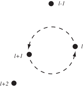
Figure 1: Interchange of the $l$-th string and the $l+1$-th string.

In this process, the axion filed $\Phi$ starts at Eq.(18) and gradually changes then finally returns to the same value (18). Generally, the wave function $u_{p}$ with $E_{p}>0$ acquires the (non-abelian) Berry phase $\gamma$ in this process,

$$u_{p}\rightarrow\sum_{E_{p^{\prime}}=E_{p}>0}(e^{i\gamma})_{p,p^{\prime}}u_{p^{\prime}}.$$ (36)

As $b_{p}$ is given by

$$b_{p}=\int dxu_{p}^{\dagger}(x)\psi_{M}(0,x),$$ (37)

then

$$b_{p}\rightarrow\sum_{E_{p^{\prime}}=E_{p}}b_{p^{\prime}}(e^{-i\gamma})_{p^{\prime},p}.$$ (38)

The annihilation operators $b_{p}$’s do not transform to the creation operators $b_{p}^{\dagger}$’s, so Eq.(29) holds after the interchange.

For the zero modes, the transformation law under the interchange can be calculated explicitly from Eq.(20): The phases of the zero modes $u_{0}^{(l)}$ and $u_{0}^{(l+1)}$ transform as

$$\phi(X_{l}-X_{l+1})\rightarrow\phi(X_{l+1}-X_{l}),\quad\phi(X_{l+1}-X_{l})\rightarrow\phi(X_{l}-X_{l+1})+2\pi,$$ (39)

so we find

$$u_{0}^{(l)}\rightarrow u_{0}^{(l+1)},\quad u_{0}^{(l+1)}\rightarrow-u_{0}^{(l)}.$$ (40)

Using the equations

$$c_{0}^{(l)}=\int dxu_{0}^{(l)\dagger}(x)\psi_{M}(0,x),\quad c_{0}^{(l+1)}=\int dxu_{0}^{(l+1)\dagger}(x)\psi_{M}(0,x),$$ (41)

we obtain

$$c_{0}^{(l)}\rightarrow c_{0}^{(l+1)},\quad c_{0}^{(l+1)}\rightarrow-c_{0}^{(l)}.$$ (42)

For $i\neq l$ and $l+1$, the phase of the zero mode $u_{0}^{(i)}$ does not change by the interchange, so $u_{0}^{(i)}$ transforms trivially

$$u_{0}^{(i)}\rightarrow u_{0}^{(i)},\quad(i\neq l,l+1),$$ (43)

and

$$c_{0}^{(i)}\rightarrow c_{0}^{(i)},\quad(i\neq l,l+1).$$ (44)

It is remarkable here that these transformation affects the condition on the state $|X_{1},\cdots,X_{n}\rangle$ given by Eq.(32). By an interchange of the $2I$-th and the $2I+1$-th strings, we find

$$d_{0}^{(I)} = \frac{1}{\sqrt{2}}\left(c_{0}^{(2I-1)}+ic_{0}^{(2I)}\right)$$ (45)

$$\rightarrow \frac{1}{\sqrt{2}}\left(c_{0}^{(2I-1)}+ic_{0}^{(2I+1)}\right)=\frac{1}{2}\left(d_{0}^{(I)}+d_{0}^{(I)\dagger}+id_{0}^{(I+1)}+id_{0}^{(I+1)\dagger}\right),$$

$$d_{0}^{(I+1)} = \frac{1}{\sqrt{2}}\left(c_{0}^{(2I+1)}+ic_{0}^{(2I+2)}\right)$$ (46)

$$\rightarrow \frac{1}{\sqrt{2}}\left(-c_{0}^{(2I)}+ic_{0}^{(2I+2)}\right)=\frac{1}{2}\left(id_{0}^{(I)}-id_{0}^{(I)\dagger}+d_{0}^{(I+1)}-d_{0}^{(I+1)\dagger}\right).$$

Thus the condition (32) is not satisfied after the interchanges. The state after the interchange must vanish by the action of the right hand side of the above equations, so we can write down the following transformation law,

$$|X_{1},\cdots,X_{n}\rangle$$

$$\rightarrow\frac{e^{i\theta_{2I,2I+1}}}{\sqrt{2}}\left(|X_{1},\cdots,X_{n}\rangle-id_{0}^{(I)\dagger}d_{0}^{(I+1)\dagger}|X_{1},\cdots,X_{n}\rangle\right),$$ (47)

where $\theta_{2I,2I+1}$ is a real constant.

Non-abelian properties of the transformations above can be easily seen by considering an interchange of $2I$-th and $2I+1$-th strings and that of $2I-1$-th and $2I$-th strings simultaneously. By an interchange of $2I-1$-th and $2I$-th strings, $d_{0}^{(I)}$ transforms as

$$d^{(I)}_{0} = \frac{1}{\sqrt{2}}\left(c_{0}^{(2I-1)}+ic_{0}^{(2I)}\right)$$ (48)

$$\rightarrow \frac{1}{\sqrt{2}}\left(c_{0}^{(2I)}-ic_{0}^{(2I-1)}\right)=-id_{0}^{(I)},$$

so the lowest state transforms as

$$|X_{1},\cdots,X_{n}\rangle\rightarrow e^{i\theta_{2I-1,2I}}|X_{1},\cdots,X_{n}\rangle,$$ (49)

where $\theta_{2I-1,2I}$ is a real constant. Thus if we interchange $2I-1$-th and $2I$-th strings first then interchange $2I$-th and $2I+1$-th strings, we obtain

$$|X_{1},\cdots,X_{n}\rangle$$

$$\rightarrow\frac{e^{i\theta_{2I-1,2I}+i\theta_{2I,2I+1}}}{\sqrt{2}}\left(|X_{1},\cdots,X_{n}\rangle-id_{0}^{(I)\dagger}d_{0}^{(I+1)\dagger}|X_{1},\cdots,X_{n}\rangle\right).$$ (50)

On the other hand, if we interchange $2I$-th and $2I+1$-th strings first then interchange $2I-1$-th and $2I$-th strings, we obtain

$$|X_{1},\cdots,X_{n}\rangle$$

$$\rightarrow\frac{e^{i\theta_{2I-1,2I}+i\theta_{2I,2I+1}}}{\sqrt{2}}\left(|X_{1},\cdots,X_{n}\rangle+d_{0}^{(I)\dagger}d_{0}^{(I+1)\dagger}|X_{1},\cdots,X_{n}\rangle\right).$$ (51)

Therefore, the interchange of $2I-1$-th and $2I$-th strings does not commute with that of $2I$-th and $2I+1$-th strings. The strings obeys non-abelian statistics.

The interchanges of the $l$-th and $l+1$-th strings can be summarized by the following unitary operator $T_{l}$:

$$T_{l}=e^{i\alpha_{l,l+1}}\cdot e^{-i\sum_{E_{p}=E_{p^{\prime}}}\gamma_{p,p^{\prime}}b_{p}b_{p^{\prime}}^{\dagger}}\cdot e^{i\frac{\pi}{4}\Sigma_{l,l+1}}.$$ (52)

Here $\Sigma_{l,l+1}=i[c_{0}^{(l)},c_{0}^{(l+1)}]$ is the generator of SO($n$) rotation in $l-(l+1)$ plane, and $\alpha_{l,l+1}$ is a real constant. The operator ${\cal O}(=c_{0}^{(i)},b_{p})$ transforms as ${\cal O}\rightarrow T_{l}{\cal O}T_{l}^{\dagger}$, and the state $|\,\,\,\rangle$ transforms as $|\,\,\,\rangle\rightarrow T_{l}|\,\,\,\rangle$. The interchange operator $T_{l}$ is the same as that of the spinor braiding statistics found in a fractional quantum Hall system [12, 13] up to a phase factor and the massive mode contributions. It is easily shown that $T_{l}$’s are generators of the braid group [17].

$$T_{l}T_{m}T_{l}=T_{m}T_{l}T_{m},\quad(|l-m|=1),$$ (53)

$$T_{l}T_{m}=T_{m}T_{l},\quad(|l-m|>1).$$ (54)

In the above, we have considered a model with a spontaneously broken global U(1) symmetry (7), but a gauged version of our model is also possible. The gauged U(1) symmetry appears to be anomalous when only the fermion spectrum is considered, but the anomaly can be cancelled by introducing an additional anti-symmetric field $B_{\mu\nu}$ and using a variety of the Green-Schwartz mechanism [15]. This “anomalous” U(1) symmetry may arise naturally in superstring compactification [18]. Strings in the gauged version of our model also obey non-abelian statistics by the similar mechanism given above.

It has been shown that unusual statistics is possible for string loops in 1+3 dimensions [19]. It is plausible that the axion strings we considered here realize this statistics non-trivially.

The author would like to thank M. Shibata and S. Yahikozawa for discussions. This work was supported in part by the Grant-in-Aid for Scientific Research No.14740158.

References

• [1] R. Jackiw and C. Rebbi, Phys. Rev. D13 (1976) 3398.
• [2] G.’t Hooft, Phys. Rev. Lett. 37 (1976) 8.
• [3] E. Witten, Nucl. Phys. B249 (1985) 557.
• [4] V.A. Rubakov, Nucl. Phys. B203 (1982) 311.
• [5] C.G. Callan Jr., Phys. Rev. D26 (1982) 2058.
• [6] M. Sato, Phys. Lett. B376 (1996) 41.
• [7] F. Wilczek and Y.S. Wu, Phys. Rev. Lett. 65 (1990) 13.
• [8] M. Bucher, Nucl. Phys. B350 (1991) 163.
• [9] F.A. Bais, P. van Driel, and M. de Wild Proptius, Phys. Lett. B280 (1992) 63; Nucl. Phys. B393 (1993) 547.
• [10] H-K. Lo and J. Preskill, Phys. Rev. D48 (1993) 4821 and references therein.
• [11] G. Moore and N. Read, Nucl. Phys. B360 (1991) 362.
• [12] C. Nayak and F. Wilczek, Nucl. Phys. B479 (1996) 529.
• [13] D.A. Ivanov, Phys. Rev. Lett. 86 (2001) 268.
• [14] C.G. Callan Jr. and J.A. Harvey, Nucl. Phys. B250 (1985) 427.
• [15] J.A. Harvey and S.G. Naculich, Phys. Lett. B217 (1989) 231.
• [16] G.W. Semenoff, Phys. Rev. D37 (1988) 2838.
• [17] See, e.g., L.H. Kauffman, Knots and Physics, (World Scientific, Singapore, 1991)
• [18] M. Dine, N. Seiberg, and E. Witten Nucl. Phys. B289 (1987) 589.
• [19] A.P. Balachandran, G. Marmo, B.S. Skagerstam, and A. Stern, Classical Topology and Quantum States, (World Scientific, Singapore, 1991), chapter 22.